VIIRS Nighttime Light Data for Income Estimation at Local Level


1
Faculty of Geography, Babeş-Bolyai University, 5-7 Clinicilor Street, 400006 Cluj-Napoca, Romania
2
World and Regional Economics Department, University of Miskolc, 3515 Miskolc-Egyetemváros, Hungary
*
Author to whom correspondence should be addressed.
Remote Sens. 2020, 12(18), 2950; https://doi.org/10.3390/rs12182950
Submission received: 19 June 2020
/
Revised: 7 September 2020
/
Accepted: 9 September 2020
/
Published: 11 September 2020
(This article belongs to the Special Issue 2nd Edition Instrumenting Smart City Applications with Big Sensing and Earth Observatory Data: Tools, Methods and Techniques)
Abstract
:The aim of the paper is to develop a model for the real-time estimation of local level income data by combining machine learning, Earth Observation, and Geographic Information System. More exactly, we estimated the income per capita by help of a machine learning model for 46 cities with more than 50,000 inhabitants, based on the National Polar-orbiting Partnership–Visible Infrared Imaging Radiometer Suite (NPP-VIIRS) nighttime satellite images from 2012–2018. For the automation of calculation, a new ModelBuilder type tool was developed within the ArcGIS software called EO-Incity (Earth Observation–Income city). The sum of light (SOL) data extracted by means of the EO-Incity tool and the observed income data were integrated in an algorithm within the MATLAB software in order to calculate a transfer equation and the average error. The results achieved were subsequently reintegrated in EO-Incity and used for the estimation of the income value at local level. The regression analyses highlighted a stable and strong relationship between SOL and income for the analyzed cities. The EO-Incity tool and the machine learning model proved to be efficient in the real-time estimation of the income at local level. When integrated in the information systems specific for smart cities, they can serve as a support for decision-making in order to fight poverty and reduce social inequalities.
1. Introduction
Over the last two decades, due to rapid digitalization and technological development, the “smart city” concept has been widely used both in the scientific literature and international policies. Despite the history and popularity of the concept there is neither a unique, nor a one-size-fits-all definition for it [1]. As cities are engines of economic growth, accounting for 80% of the global Gross Domestic Product (GDP) [2], they also have a significant impact on social and economic welfare, thus being considered key elements for tackling future challenges. This is also highlighted by the fact that more than half of the global population lives in urban areas (in Europe more than 75 percent), a ratio which is constantly increasing [2]. All these lead to an increased consumption of resources in cities (mainly consumption of energy resources), placing a significant impact on the surrounding environment and on urban sustainability.
Despite the fact that smart cities do have different interpretations [3,4,5,6,7,8,9,10] and have also attracted criticism [11,12,13,14,15,16], it seems that the concept has established itself by becoming embedded in the scientific literature, with ever increasing practical applications. Along the years it has become a widely used policy concept for cities, its popularity being supported by its perceived connection to the globally accepted Sustainable Development Goals [17].
Cities are constantly changing, thereby continuously presenting city managers with new challenges in order to transform urban areas into more livable spaces. The key to successfully adapt to these changes is in the hands of local authorities, which have the responsibility to provide accurate and timely spatial information for monitoring, managing, and planning of urban areas [18,19]. Therefore, the smart city concept takes a holistic approach to utilizing information technologies combined with real-time analysis methods, paving the way towards a more sustainable economic development. This holistic view of cities made possible by Earth Observation (EO) offers a useful alternative to data collection over spatial units; thus, allowing a reliable way of gathering spatial data for monitoring the rapidly changing urban areas [20,21]. Satellite-based EO data can help fill some of the gaps in the tools, but also gather useful data and knowledge we need in cities.
2. Research Overview
Scientific literature reveals a great variety of applications for EO data not only in analyzing the environmental changes, but also in applying it in regional science. Musakwa and Niekerk [22] have monitored sustainable urban development using built-up area indicators. Patino and Duque [23] reviewed the potential applications of satellite remote sensing to regional science research in urban settings by focusing on social problems with a spatial dimension. Application of EO can also be found in assessing social inequality and quality of life by detecting and monitoring the formation of slums [24,25], urban growth and urban sustainability [26,27], but also the estimation of population or GDP [28,29,30]. These studies highlighted the big challenges of EO data in supporting sustainable urban research and policy development.
The remote sensing and the Geographical Information System (GIS) can provide new perspectives for the assessment of the economic performances both at national and at sub-national level. Over the last period, increasing attention was paid to the usage of nighttime satellite images for the extraction of the socio-economic data corresponding to a certain spatial unit, when this data is missing or has a low quality. In terms of income per capita prediction, Ebener et al. [31] developed a global model based on the DMPS-OLS satellite images, achieving promising results both at national and at sub-national level. Subsequently, Li et al. [32], after studying the relationship between the Nighttime lights (NTL) data and the economic indicators, noticed that the NPP-VIIRS data has a better capacity for the prediction of the gross regional product (GRP) than the Defense Meteorological Satellite Program—Operational Linescan System (DMSP-OLS) data. In the case of the present study, too, the NPP-VIIRS data proved to be a good starting point in estimating the income at local level.
The nighttime light data captured by the satellites in order to assess the economic development is very actual and it is used in many studies lately [29,33,34]. Dai et al. [35] estimated the GDP for 31 provinces and 341 cities in the mainland China, based on the DMSP-OLS and NPP/VIIRS satellite data and on the existing statistical data. As a result of comparing the accuracy of the results, we noticed that the DMSP-OLS data can be used for the estimation of the GDP at province level exclusively, while the NPP/VIIRS data can be used both at province and at local (cities) level. Basihos [36] estimated the GDP at sub-national level in Turkey for the 2001–2013 period, based on nightlights, using the neural network algorithm and rebuilt the GDP series for the 1992–2001 period, achieving statistically significant results.
The machine learning model was also used successfully by Jean et al. [37] in estimating consumption expenditure for five countries in Africa based on the satellite images. Määttä and Lessmann [38] applied the random forest machine learning algorithm with a view to predict whether the light corresponding to a pixel in DMPS-OLS nightlight data is of human origin or not; thus, creating a Human Lights product. The machine learning algorithms (artificial neural network) were used by Subash et al. [39] to predict poverty at sub-national level in India based on the DMPS-OLS nightlight data. The NTL dataset is not only useful in updating the analysis of connecting nighttime lighting patterns with income inequalities, but also serves the purpose of validating the robustness of our identification and estimation strategy. Our analysis is in line with this mainstream research using nighttime lights datasets (NPP-VIIRS) and machine learning model for Romanian cities from 2012 to 2018 and for Hungarian cities from 2014 to 2016, in order to estimate per capita income. For this purpose, we selected 46 Romanian cities and 19 Hungarian cities with a population over 50,000 inhabitants. There is a direct and positive correlation between the size and the economic complexity of cities; that means bigger cities have more complex economic functions, related to industries and a wide variety of services, while smaller cities have a large agricultural sector or one dominant industry (for example, mining) or service function (generally tourism) [40,41]. For these reasons, there is no significant correlation between the economic output of smaller cities and night lights, the latter being largely generated by industries and service-related functions [30].
The analysis is expected to contribute to the development of novel methods for improved EO-based urban services to support smart and sustainable urban development. This study proposes a new tool (abbreviated EO-Incity in this study) designed to estimate the income at sub-national level based on the nighttime satellite images.
3. Study Area and Data
3.1. Study Area
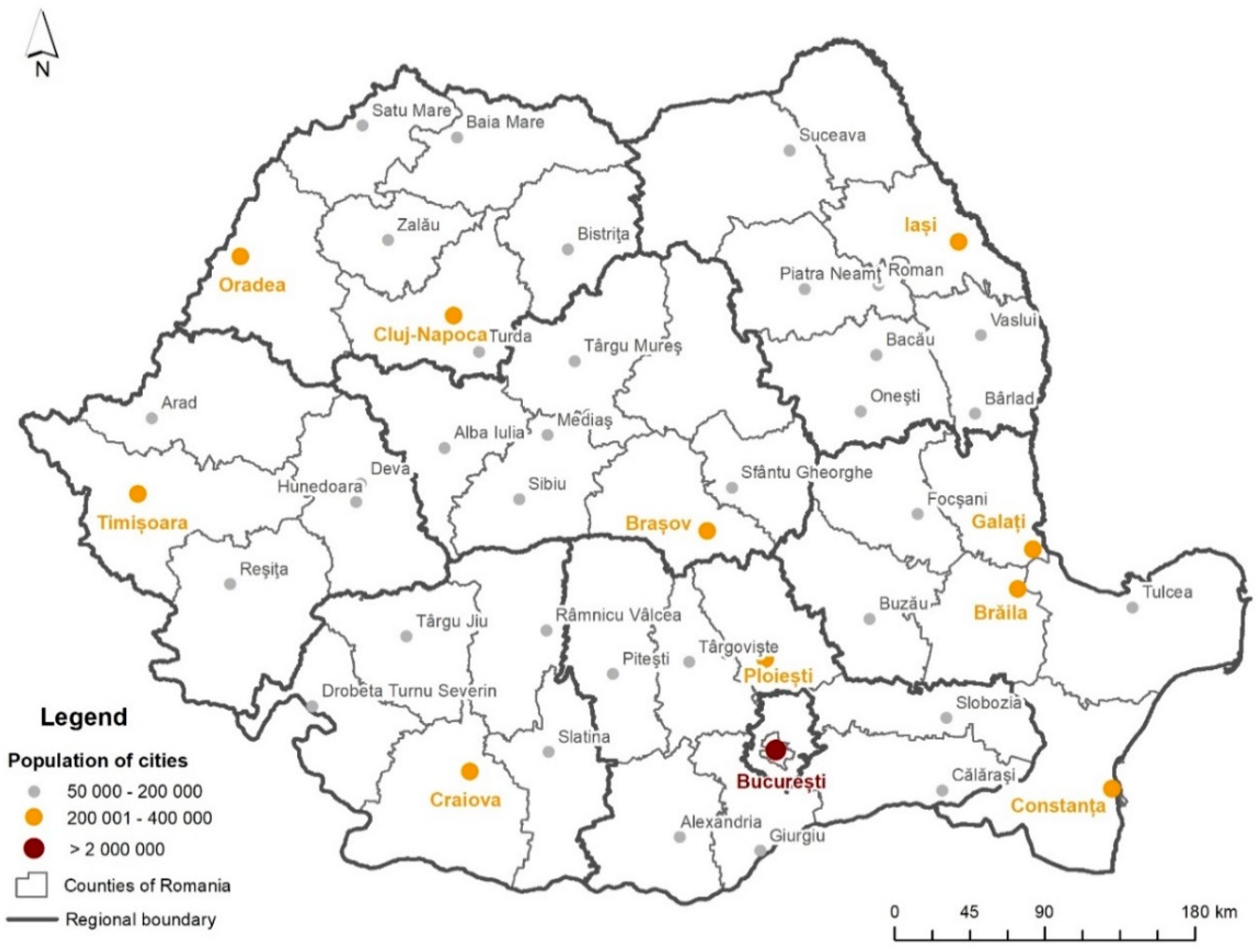
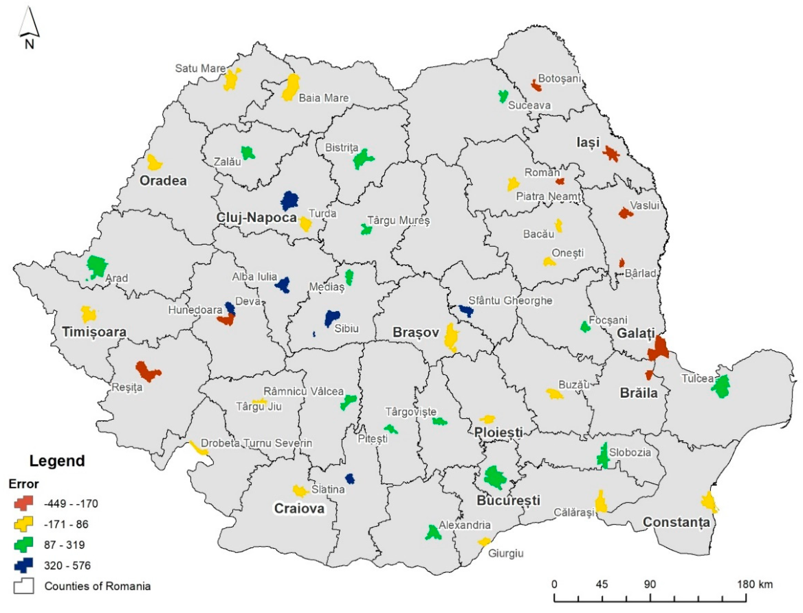
Romania is organized into eight development regions (NUTS-2), 41 counties, and the Municipality of Bucharest (NUTS-3) and 3181 LAU1 (local administrative units: communes and cities). For this research, we have selected 46 municipalities and cities (LAU1) with a population of more than 50,000 inhabitants (Appendix C), of the total 103 municipalities and 216 cities in Romania (Figure 1). These cities are the major economic hubs of the country [42,43,44], especially the capital—the Municipality of Bucharest—the sixth city in the EU in terms of population (2,131,034 inhabitants in 2019), followed by six regional centers with a population exceeding 300,000 inhabitants: Iași (378,954 inhabitants), Timișoara (328,186 inhabitants), Cluj-Napoca (324,960 inhabitants), Constanța (313,021 inhabitants), Galați (304,050 inhabitants), and Craiova (301,269 inhabitants) [45].
3.2. Data Collection
Within this research we used the NPP-VIIRS images [48] produced by the Earth Observations Group (EOG) at NOAA/NCEI (National Centers for Environmental Information) with a 15 arc seconds (approximately 500 m) resolution for income estimation al local level in Romania. The VIIRS (Visible Infrared Imaging Radiometer Suite) sensor of the Suomi NPP (National Polar-Orbiting Partnership) satellite records the intensity of the lights and collects data in 22 different spectral bands, of which one is the DNB (Day/Night Band) band. The Suomi NPP satellite was launched on the 28 October 2011. The VIIRS instrument onboard the Suomi NPP satellite collects global observations, which span over the visible and infrared wavelengths. Day/Night band hosted by VIIRS allows for the observation of nighttime lights with a 15 arc second spatial resolutions. Using nighttime data from the VIIRS Day/Night Band, a suite of average radiance composite images is produced. These composites are available at a monthly scale for the 2012–2019 period and at an annual scale for 2015 and 2016. In the present study, we used the monthly data. There are two configurations of the NPP-VIIRS monthly composites: “vcmslcfg”—where data contaminated by stray light are corrected and “vcmcfg”—where data contaminated by stray light are removed [49]. We have used the “vcmslcfg” layer. Based on the satellite images available on a monthly basis, an annual average pixel brightness was calculated using the “vcmslcfg” layer, resulting in seven composite VIIRS nighttime light images. An image has thus been produced for each year corresponding to the 2012–2018 period. Subsequently, the sum of light (SOL) calculation was conducted by means of the ArcGIS 10.1 software (Environmental Systems Research Institute, Redlands, CA, USA) for each administrative territorial unit in Romania, which was later used as an input in calculating the local income. The sum of light (SOL) was extracted by summing all pixel values of the nighttime light image in each administrative territorial unit.
The permanent resident population data by localities was obtained from the National Institute of Statistics [45] for the 2012–2018 period. The local tax income data for each administrative territorial unit were extracted from the MRDPA (Ministry of Regional Development and Public Administration) database for the 2012–2018 period [50] and are expressed in Romanian leu (1 RON = 0.21 EUR, June 2020). Subsequently, the local tax income data was calculated per person.
4. Methodology
Several studies highlighted a positive statistical relationship between the NTL data and GDP, both at national level and at sub-national level [33,34,35,51,52]. For Romania, Ivan et al. [30] noticed a strong relationship between NTL and income, as well as between NTL and the GDP at county level [53]. The NTL data was correlated best with the income, which indicated its high potential to estimate the income at sub-national level.
The research on the relationship between SOL and local income for each administrative territorial unit of Romania (3181) highlighted a strong relationship (Pearson correlation coefficient ≥ 0.82, R2 > 0.68) between the two variables for the municipalities and cities with population exceeding 50,000 inhabitants (46 cities) (Table 1).
Based on these findings we used the local income estimation for the year 2018 for the 46 cities in Romania using a machine learning model within the MATLAB software.
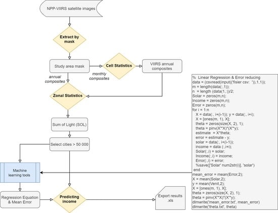
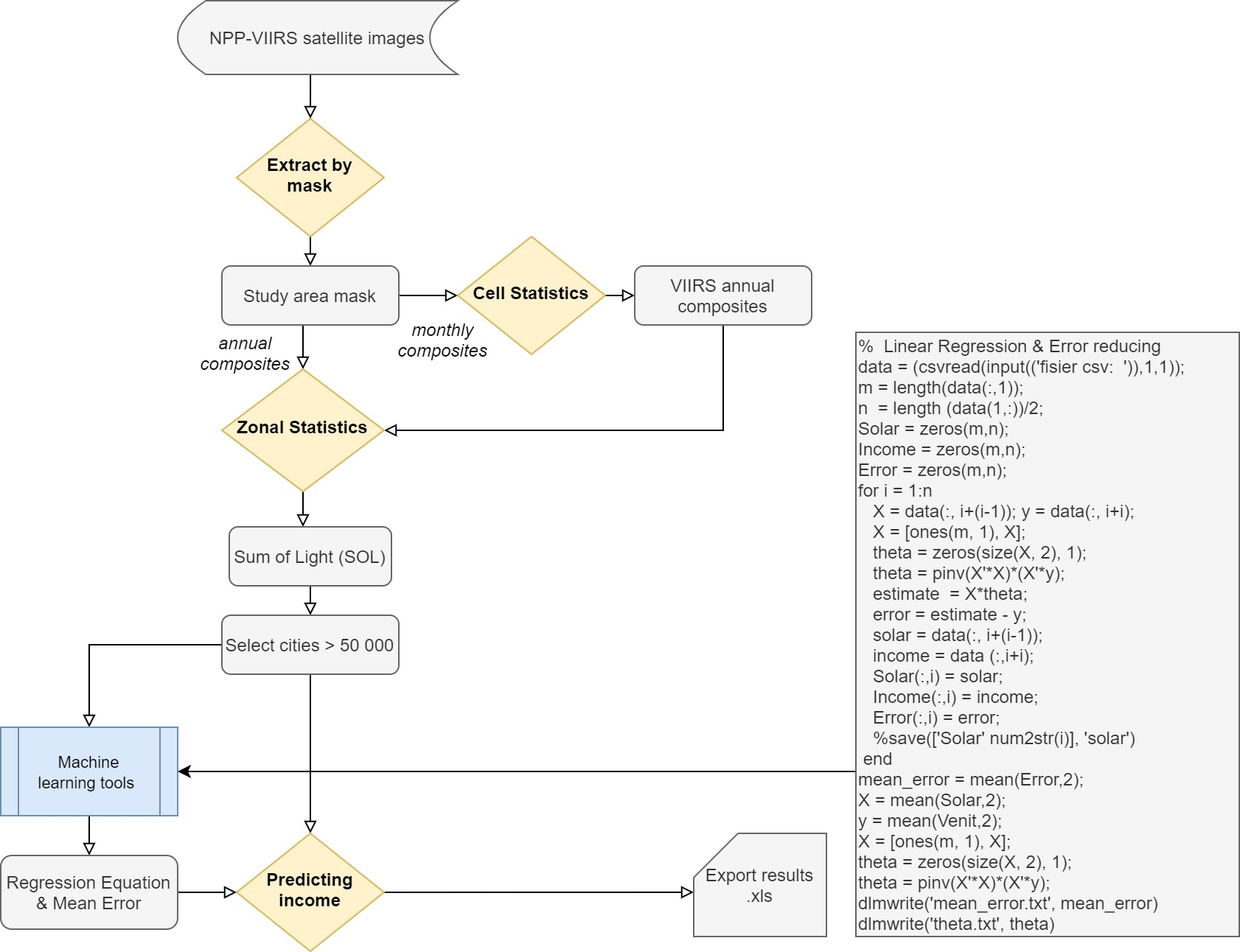
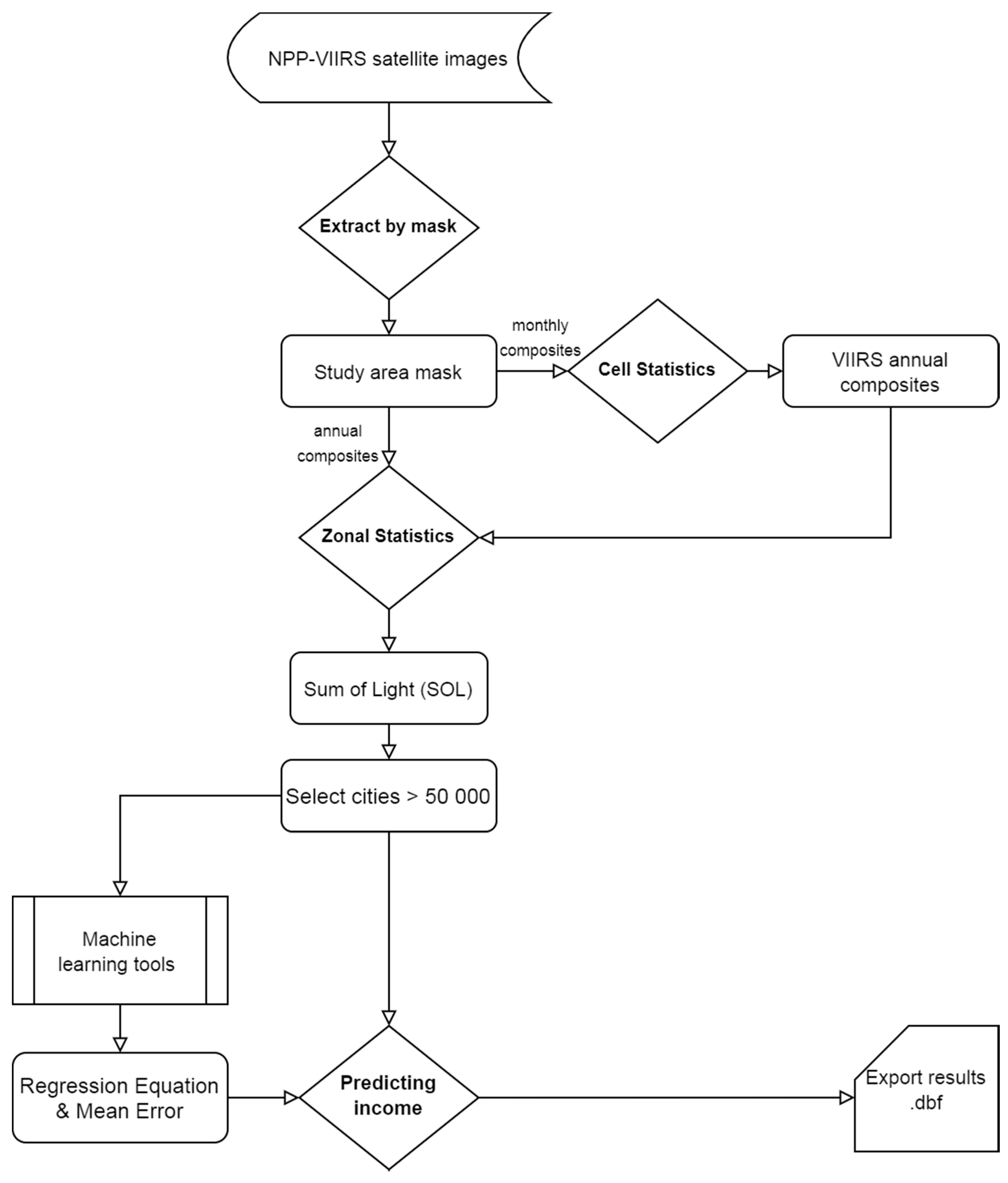
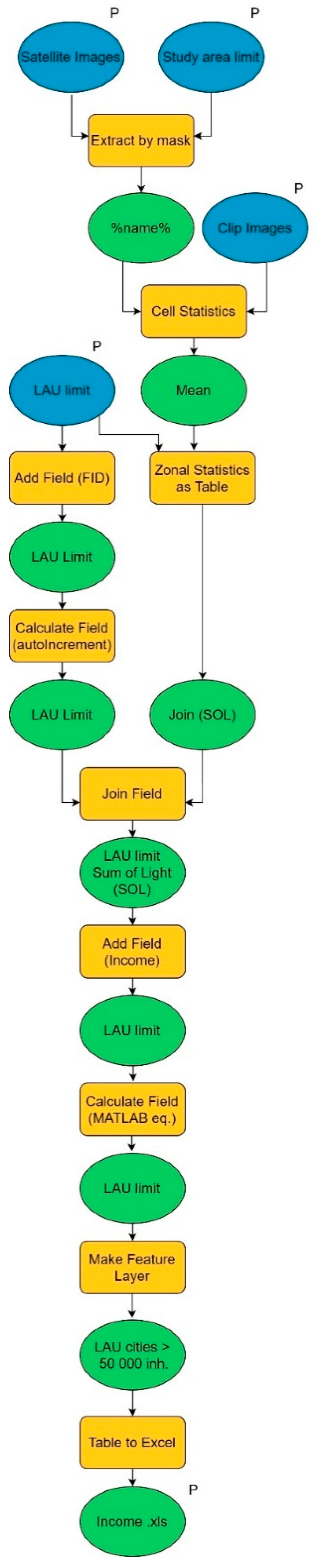
For the automation of the calculation we proceeded to the development of a ModelBuilder type tool in the ArcGIS software (Figure 2). The tool was called EO-Incity (Earth Observation–Income city). The Model Builder is a visual programing language, where geoprocessing and data processing tools can be interactively combined to create a workflow. For the creation of the model two sub-models were first developed: the first to mask the study area using the “Extract by Mask” tool and the second sub-model to calculate the annual average (for the images available on a monthly basis) using the “Cell Statistics” tool. The “Extract by Mask” tool extracts the cells of a raster, which correspond to a country limit defined by the input mask, while the “Cell Statistics” tool calculates a per-cell statistic (mean in our case) from 12 monthly rasters.
In order to calculate the sum of light (SOL) for each individual administrative territorial unit, the “Zonal Statistics as Table” tool was used. The “Zonal Statistics as Table” tool calculates statistics (sum in our case) on the values of a raster within each administrative territorial unit. The data preparation process involves the following processes: (1) masking the downloaded raw monthly VIIRS satellite images (vcmslcfg layer) using the limit of the study area (country limit in our case); (2) calculating an average annual pixel brightness for the 12 masked monthly images, resulting a single nighttime light image; and (3) summing up the pixel values of the image for each territorial administrative unit, resulting the sum of light (SOL) values for each city. In case of annual images, step (2) was skipped. The EO-Incity tool in the first part of the model masks the study area and calculate the SOL, using as input data the annual or monthly VIIRS satellite images. In the second part of the model it uses as input parameters the calculated SOL data and the equation resulting from running the algorithm within MATLAB for the estimation of the income. (Appendix A).
In the MATLAB software, the calculation algorithm transposed in a script involves on the one hand the achievement of the parameters of a transfer function for the estimation of the income based on the nighttime satellite images and, on the other hand, the calculation of the average error (Appendix B). The input comes from the EO-Incity tool and it is represented by the sum of light (SOL) and the per capita income corresponding to the cities that exceed a certain population threshold (for this particular study, the cities with a population over 50,000 inhabitants). The parameters of the transfer equation are calculated integrating all the annual value sets generated from satellite images and by the processing of the income data in one-step learning algorithm. The normal equation was chosen because it is an efficient and fast calculation manner due to the analytical approach of the linear regression:
where θ—parameters of the linear regression; X—the matrix which contains the independent variables; and y—the matrix containing the dependent variables.
θ = (XTX)−1(XTy)
The same normal equation is used for the calculation of the errors of linear regressions for each annual set of values. The errors for each year are then mediated for the entire calculation period.
where Ej—the values estimated using the regression equation for year j; θj—the parameters of the linear regression for year j; Xj—the independent variable for year j; yj—the dependent variable for year j; εj—the error of linear regression for year j; and ε—the average error; n—number of years.
Ej = θjXj
εj = Ej − yj
The output of the MATLAB script is then reintegrated in EO-Incity and used for the estimation of the income values based on satellite data (SOL) for the years when this data is not available for the reduction of errors. The income data resulting from running the EO-Incity tool are saved in.dbf format, which makes them easy to view and process.
We used the linear regression model in order to test the relationship between the estimated income and night time light/observed income, which is described mathematically in the form:
where y represents the dependent variable (in our case the estimated income); x represents the independent variable (representing the SOL/observed income); β0 is the so-called intercept of the model—the expected value of y when all the x’s are zero; β1 is the coefficient (multiplier) of the variable xi; and ε is the residual variable (the mean or expected value of y for a given value of x). The betas together with the mean and standard deviation of the y are the parameters of the model.
y = β0 + β1x + ε
In order to find out the accuracy in regression models, R2 and its adjusted counterpart aR2 are highlighted, deriving from the regression equation to quantify model performance. While the R2 shows the validity of the chosen model for explaining the variation of Y (the percentage of income estimation explained by the NTL), adjusted R2 is a correction to the R2 that takes into account the number of variables used in the model. The higher the R-squared, the better the model.
The predictive ability of the model is often tested by using the relative error (RE) or residuals (the difference between the observed y values and the predicted y values) and relative root mean square error (RMSE). RMSE measures the average error performed by the model in predicting the outcome for an observation. As the square root of a variance, RMSE can be interpreted as the standard deviation of the unexplained variance and it has the useful property of being in the same units as the response variable. RMSE provides a good picture of how accurately the response is predicted by the model and it is the most important criterion for fit if prediction is the main purpose of the model. In this sense, lower values of RMSE indicate better fit.
Additionally, Akaike information criterion (AIC) is a fined technique based on in-sample fit to estimate the likelihood of a model to predict/estimate the future values. The basic formula is defined as
where K is the number of model parameters (the number of variables in the model plus the intercept) and Log-likelihood is a measure of model fit. The basic idea of AIC is to penalize the inclusion of additional variables to a model which, in fact, increases the error. The lower the AIC, the better the model.
AIC = −2(log-likelihood) + 2K
{\displaystyle a,a+\Delta x,a+2\,\Delta x,\ldots ,a+(n-2)\,\Delta x,a+(n-1)\,\Delta x,b.}
5. Results
In the socio-economic calculations the income represents an important parameter for decision-making in order to fight poverty and reduce social inequalities. On the annual scale, an offset occurs between the statistically reported data and the specific budgetary projection. Our instrument offers the possibility of real-time estimation of this data at local level by means of Earth Observation (EO).
As a result of running the EO-Incity tool for the cities with more than 50,000 inhabitants in Romania, we achieved an estimation of the income for the year 2018. After comparing the estimated results, we achieved a regression coefficient of 0.86 that explains 75% of the total variation and a root square mean error (RMSE) of 247.
Taking into consideration the values of the regression values, the highest negative differences (overestimation) are noticed for the cities in the east of Romania (Figure 3). The possible source of error is the overestimation of the population due to the practice of the citizens in the Republic of Moldova to declare their presence in these cities (Vaslui, Bârlad, Iași) to obtain Romanian citizenship [54,55,56]. As for the positive difference (underestimation), the largest differences were noticed in Slatina, where there is a big electricity consumer, the largest aluminum producer in Europe, Alro SA, which also generates higher SOL values. In the case of the cities of Sibiu, Deva, Cluj-Napoca, and Sfântu Gheorghe, a possible explanation would be the underestimation of the resident population or/and informal economy (see for this subject Ghosh et al. [33]). In the case of Cluj-Napoca—one of the most important academic centers in Romania—another explanation would be the large number of students present, but registered as residents elsewhere. The positive difference in Cluj-Napoca and other cities like Sibiu and Brasov may also be explained by tourism. Bluhm and Klaus [57] pointed out that stable lights may underestimate income in high-density places, therefore they recommend using top-coding correction. In our analysis we have found several cities of similar size (e.g., Cluj and Iasi; Braila and Sibiu) where over- and underestimation of income per capita was related to the specific characteristics of Romanian cities mentioned above and not necessarily to the high density of the population. This is also backed by the fact that in the largest agglomeration area (the capital city, Bucharest with 1.9 million inhabitant), underestimation was not that significant.
The linear regression parameters between the estimated income and the observed income for each year during the 2012–2018 period remained close to the values in 2018 (Figure 4). Thus, the value of the R2 coefficient was located between 0.68 in 2017 and 0.76 in 2013, which illustrates a stable relation in time between the two variables (SOL and income). In the context of these findings, we proceeded to error reduction in order to improve the prediction. A good strategy for improving the prediction is to minimize the term ε in Equation (5) as much as possible [58]. We intend to use error-related information for the common period with satellite and revenue data to characterize the specific error for each particular case (city). The mean error achieved by the mediation of the regression errors each year is applied to the values estimated for the year 2018.
Table 2 shows a significant improvement of the correlation coefficient between the estimated and the observed values, which in this case exceeds the value of 0.93, while the total explained variability increases from 75 to 87%. RMSE is significantly reduced from 247 to 181.
As a result of the European Union’s efforts to reduce electricity consumption by 80%, both Romania and Hungary are in full transition to LED lighting. The use of this technology implies a decrease in DNB radiance.
This decrease is most often outweighed by the increase in radiance in areas around cities due to urban sprawl or the “skyglow” effect (the clear sky predominantly scatters short-wavelength light) [59]. An increase of more than three times of the scotopic illuminance outside the city was also observed in Hungary when using LED technology [60]. This study uses a radiative transfer model based on Monte Carlo simulation to make a comparison between different indicators used to qualify and predict the change in radiance in case of different scenarios related to transitions to LED lighting.
The impact of the decrease in radiance—due to LED transition—on the relationship with personal income can be limited by our methodological approach. The use of SOL attenuates the decrease in radiance observed in downtown areas. Another advantage is the use of machine learning that can adapt to such a change.
6. Validation of the Results and Discussions
In order to validate the EO-Incity tool we used the similar methodology, for the estimation of the income value at local level for Hungarian cities. The population and local tax income annual data were extracted from the Hungarian Central Statistical Office [61] for the 2014–2016 period for Hungary. The income data are expressed in Hungarian forint (1 HUF = 0.0029 EUR, June 2020) and have been reported per person.
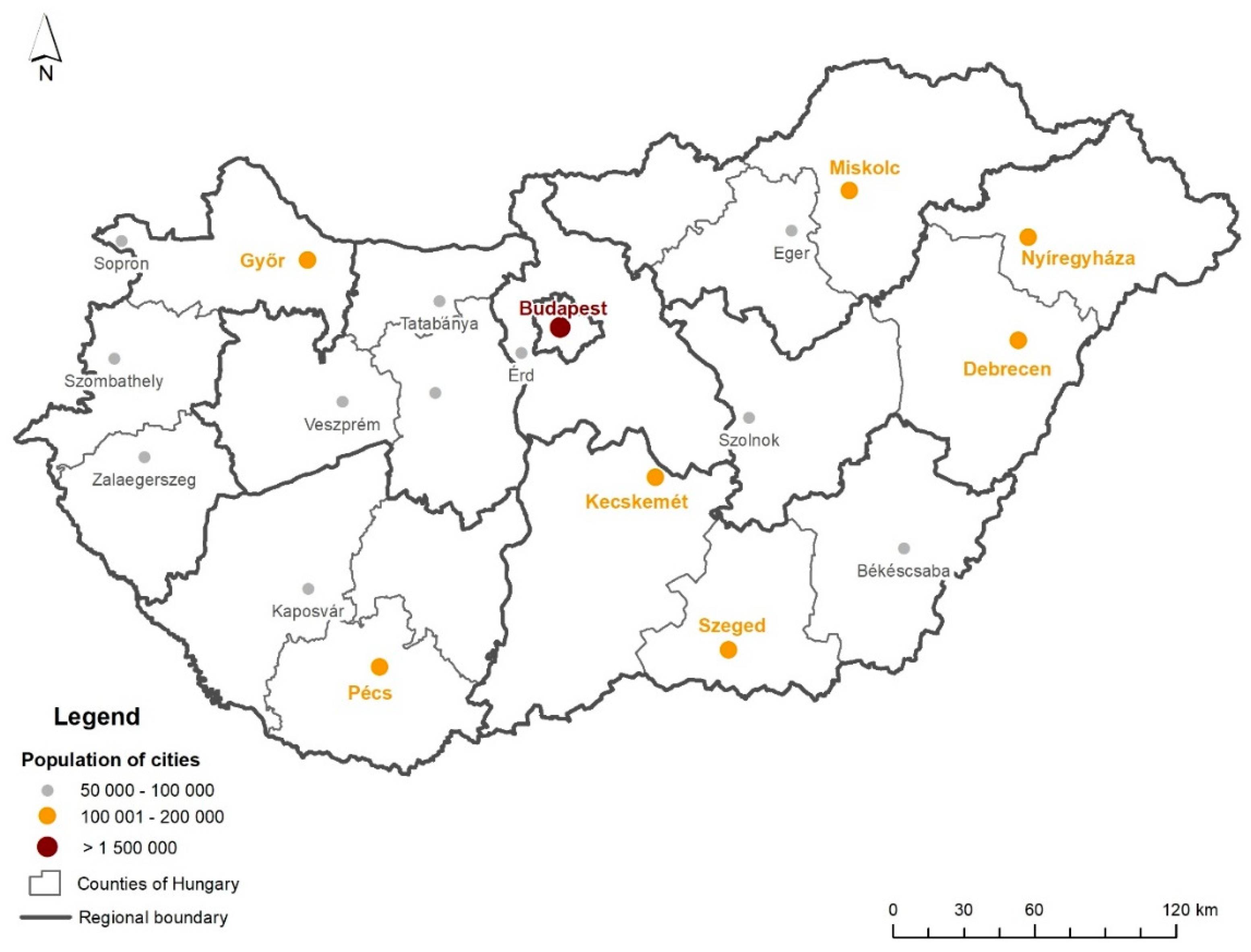
Hungary is divided into eight regions (NUTS-2), 19 counties and capital city—Budapest (NUTS-3) and 3155 LAU2 (local administrative units: settlements). In the present study, we have selected 19 municipalities and cities with a population of more than 50,000 inhabitants (Figure 5 and Appendix C). The largest cities from Hungary with a population exceeding 100,000 inhabitants are the capital city—Budapest (1,693,051 inhabitants), Debrecen (203,493 inhabitants), Szeged (163,763 inhabitants), Miskolc (160,325 inhabitants), Pécs (149,030 inhabitants), Győr (124,743 inhabitants), Nyiregyháza (120,086 inhabitants), and Kecskemét (110,974 inhabitants) [61].
Income inequalities have a clear spatial distribution in Hungary: apart from the capital city, there is a strong decrease in the income from west to east. The most developed areas can be found in the central and north-western parts of the country, with a strong peripheralization in the eastern parts. The economic spatial structure of the country has also put its mark on the cities, influencing the adoption of the “smart city” concept, which appeared mostly in the largest urban areas. The need to apply the smart city concept in urban development appeared in 2015 when a government resolution established the state regulatory and oversight responsibilities for smart city developments [62]. Since then, the spread of the smart city model has accelerated significantly in Hungary especially in the larger urban areas: the Smart city Budapest initiative has been running in the capital since 2014, Debrecen and Szeged have had a smart city vision and concept since 2016. Miskolc, while Kaposvár and Szolnok joined the Open and Agile Smart Cities organization in 2016 [63]. As the smart city concept has a strong connection with sustainable development, Hungary has also committed itself to adopt a series of sustainable development goals (SDG). In this context, the use of earth observation solutions for an improved monitoring of the SDG implementation progress has also become a subject for discussion.
We have chosen Hungary for validating our results for two reasons: on one hand, from a historical point of view, as the northern part of Romania belonged to Hungary between the two world wars, showing a strong ethnic and cultural connection with the neighboring country. Secondly, from an economic point of view, as Romania and Hungary have a strong economic collaboration: a large number of Hungarian SMEs (Small and Medium size Enterprises) have been established in Romania and vice-versa in the last years, facilitating a strong cooperation between the two countries, in addition to the several cross border cooperation projects implemented on both sides of the border. Furthermore, even though the economic profile and size of the two countries differs greatly, in the last years the two countries have shown one of the highest rates of economic growth among EU Member States (4.6% in the case of Hungary and 4.2% in case of Romania in 2019 Q4) [64].
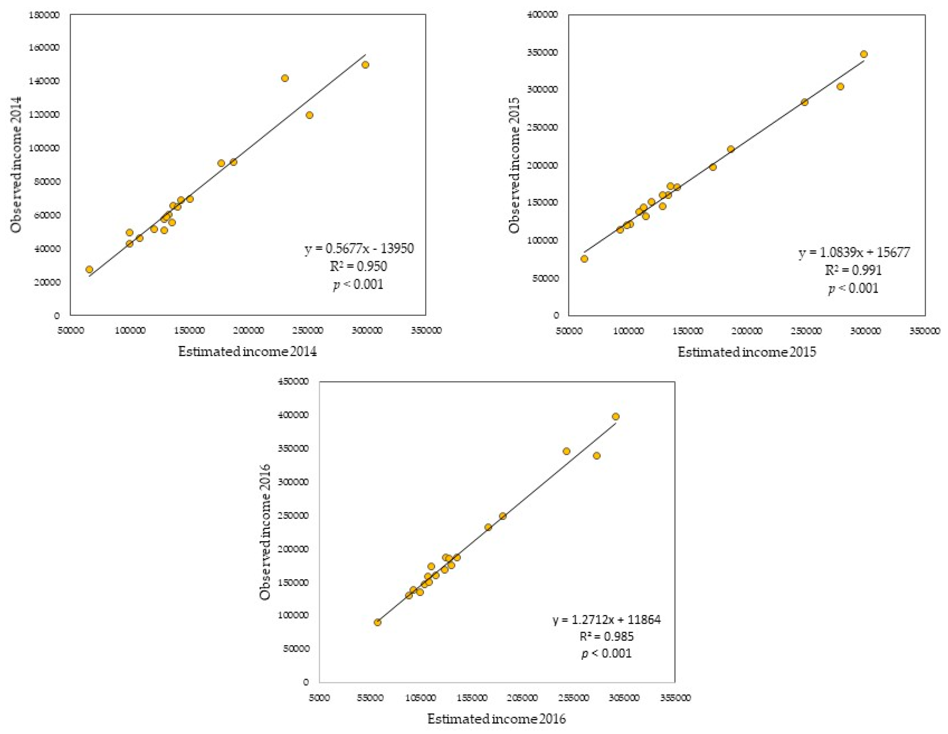
In the case of the Hungarian cities, the regression analyses highlighted a stable and strong relationship between the observed income and the estimated income (R2 > 0.95) for each year during the 2014–2016 period (Figure 6 and Table 3).
The results illustrate the validation of the methodology described in the present paper for Hungarian cities over 50,000 inhabitants. The EO-Incity tool can be used on a regional scale (being validated in Hungary as well) in filling in data gaps or collecting new data at city level. This tool created to estimate the income at local level based on the VIIRS nighttime satellite images enables fast, automated, and real-time estimation of the income. A better spatial resolution of nighttime light data would bring improvements to small-scale income estimation. Luojia1-01 nighttime light satellite images with a spatial resolution of 130 m compared to NPP/VIIRS (500 m spatial resolution) contain more information and spatial details compared to DMSP-OLS/NPP-VIIRS nighttime light data and can provide more satisfactory results on a small scale [65]. In the future, we propose to estimate the income at local level using data from the Luojia1-01 satellite, as opposed to the data obtained from the NPP-VIIRS satellite. Luojia1-01 was launched in June 2018, so the main limitation of these images compared to NPP/VIIRS is the lack of multi-temporal images, which limits their use in the analysis of time series. In addition, other valuable sources of nightlights data are represented by nighttime photographs from the International Space Station with a moderate spatial resolution (between 5 and 200 m), as well as maps of urban nighttime lights at fine spatial resolutions obtained from airborne sensors for studying socio-economic properties of cities [66].
The income estimation tool developed in the paper (EO-Incity) has not provided any evidence for a hypothetical correlation with the functional typology of the cities. However, the theoretical positive correlation between city size and the functional complexity of cities highlights the importance of overestimations in the population for cities located close to the Eastern borders of Romania and for those cities with important educational functions (Cluj-Napoca and Iași).
Limitations
Even if the correlations between income and night images are statistically representative and the explanation of the total variability are very good, currently, the extension of the estimation method on a regional scale is limited by the short period with common income data and satellite images (2014 to date).
Another limitation is the spatial inhomogeneity of cities caused by different urban development strategies from one country to another. However, we must not forget about the different methodology of reporting income data and the problems related to data reliability. We must notice also the extern causes like new lighting technologies or underestimation of income in high-density places.
The third limitation of the study is related to the resolution of NPP-VIIRS satellite images with a resolution of 500 m, compared to the resolution of Luojia1-01 images of 130 m, which do not offer a very high accuracy at the scale of urban areas. It is also necessary to compare nighttime satellite images in estimating income in high-density places before and after using top-coding correction.
A successful strategy for reducing constraints would be to introduce more cities in machine learning processing and to develop a methodology for calculating the transfer function at the regional level instead at national one.
7. Conclusions
EO-Incity proved to be an efficient tool in estimating the real-time income at local level. The results have a high potential of being integrated in the information systems specific to smart cities, as a support for decisions on the more efficient allocation of the financial resources to fight poverty and reduce inequalities. In this way, they may have an important contribution to the improvement of the city management and planning, and, indirectly, to the improvement of the quality of life in cities adopting smart solutions.
The regression analyses illustrated a very powerful relationship between SOL and income for the cities with more than 50,000 inhabitants. This finding is in line with our previous research [30], and it underlines the direct relationship between city size, the economic complexity of cities on one side, and the intensity of nightlights, on the other side. The combination of the machine learning model with the EO-Incity tool, combined with a strategy for error reduction enabled an efficient and real-time estimation of the income, which explained 87% of the total variability.
On the horizon, we wish to implement the methodology and the tool in other countries too, both in Europe and in other continents. Moreover, we intend to conduct the reconstruction of income based on this tool in the countries where the statistical reporting is not available or reliable.
Author Contributions
Conceptualization, I.T.; Data curation, K.I.; Formal analysis, J.B.; Investigation, J.B.; Methodology, K.I., I.-H.H. and I.T.; Software, I.-H.H.; Writing—original draft, K.I., I.-H.H. and I.T.; Writing—review & editing, J.B. All authors contributed equally to the research presented in this paper and to the preparation of the final manuscript. All authors have read and agreed to the published version of the manuscript.
Funding
This work was supported by a grant of Ministry of Research and Innovation, CNCS-UEFISCDI, project number PN-III-P4-ID-PCCF-2016-0084, within PNCDI III.
Acknowledgments
Thanks for the funding support.
Conflicts of Interest
The authors declare no conflict of interest.
Appendix A

Appendix B
Appendix C
| Romania | ||
| City | Population | |
| 1 | București | 2,112,483 |
| 2 | Iași | 373,507 |
| 3 | Timișoara | 330,014 |
| 4 | Cluj-Napoca | 323,484 |
| 5 | Constanța | 314,816 |
| 6 | Galați | 303,069 |
| 7 | Craiova | 302,783 |
| 8 | Brașov | 289,878 |
| 9 | Ploiești | 229,641 |
| 10 | Oradea | 221,796 |
| 11 | Brăila | 205,172 |
| 12 | Bacău | 197,285 |
| 13 | Arad | 177,464 |
| 14 | Pitești | 175,047 |
| 15 | Sibiu | 169,177 |
| 16 | Târgu Mureș | 148,490 |
| 17 | Baia Mare | 146,241 |
| 18 | Buzău | 133,376 |
| 19 | Suceava | 122,231 |
| 20 | Botoșani | 120,902 |
| 21 | Satu Mare | 120,736 |
| 22 | Râmnicu Vâlcea | 118,111 |
| 23 | Piatra Neamț | 113,396 |
| 24 | Vaslui | 113,272 |
| 25 | Drobeta Turnu Severin | 107,614 |
| 26 | Târgu Jiu | 95,869 |
| 27 | Bistrița | 93,950 |
| 28 | Focșani | 92,936 |
| 29 | Târgoviște | 92,090 |
| 30 | Tulcea | 87,698 |
| 31 | Reșița | 86,554 |
| 32 | Slatina | 83,389 |
| 33 | Călărași | 76,380 |
| 34 | Alba Iulia | 74,574 |
| 35 | Hunedoara | 72,971 |
| 36 | Bârlad | 71,431 |
| 37 | Deva | 69,527 |
| 38 | Zalău | 69,518 |
| 39 | Roman | 69,479 |
| 40 | Giurgiu | 67,721 |
| 41 | Sfântu Gheorghe | 64,428 |
| 42 | Mediaș | 57,701 |
| 43 | Turda | 56,146 |
| 44 | Slobozia | 51,999 |
| 45 | Onești | 51,580 |
| 46 | Alexandria | 50,832 |
| Hungary | ||
| City | Population | |
| 1 | Budapest | 169,3051 |
| 2 | Debrecen | 203,493 |
| 3 | Szeged | 163,763 |
| 4 | Miskolc | 160,325 |
| 5 | Pécs | 149,030 |
| 6 | Győr | 124,743 |
| 7 | Nyiregyháza | 120,086 |
| 8 | Kecskemét | 110,974 |
| 9 | Székesfehérvár | 97,190 |
| 10 | Szombathely | 76,528 |
| 11 | Szolnok | 71,084 |
| 12 | Tatabánya | 69,092 |
| 13 | Érd | 68,039 |
| 14 | Kaposvár | 63,778 |
| 15 | Békéscsaba | 60,137 |
| 16 | Sopron | 58,458 |
| 17 | Zalaegerszeg | 57,914 |
| 18 | Veszprém | 56,361 |
| 19 | Eger | 53,091 |
References
- O’Grady, M.; O’Hare, G. How Smart Is Your City? Science 2012, 335, 1581–1582. [Google Scholar] [CrossRef] [PubMed]
- United Nations. World Urbanization Prospects: The 2018 Revision. Available online: https://population.un.org/wup/Publications/Files/WUP2018-Report.pdf. (accessed on 13 February 2020).
- Caragliu, A.; Del Bo, C.; Nijkamp, P. Smart Cities in Europe. J. Urban Technol. 2011, 18, 65–82. [Google Scholar] [CrossRef]
- Schaffers, H.; Ratti, C.; Komninos, N. Special issue on smart applications for smart cities: New approaches to innovation: Guest editors’ introduction. J. Theor. Appl. Electron. Commer. Res. 2012, 7, 2–5. [Google Scholar] [CrossRef] [Green Version]
- Turcu, C. Re-thinking sustainability indicators: Local perspectives of urban sustainability. J. Environ. Plan. Manag. 2013, 56, 695–719. [Google Scholar] [CrossRef] [Green Version]
- Berardi, U. Sustainability Assessments of urban Communities through Rating Systems. Environ. Dev. Sustain. 2013, 15, 1573–1591. [Google Scholar] [CrossRef]
- Zhuhadar, L.; Thrasher, E.; Marklin, S.; de Pablos, P.O. The next wave of innovation—Review of smart cities intelligent operation systems. Comput. Hum. Behav. 2017, 66, 273–281. [Google Scholar] [CrossRef] [Green Version]
- Peng, G.; Nunes, M.; Zheng, L. Impacts of low citizen awareness and usage in smart city services: The case of London’s smart parking system. Inf. Syst. e-Bus. Manag. 2017, 15, 845–876. [Google Scholar] [CrossRef]
- Guo, J.; Ma, J.; Li, X.; Zhang, J.; Zhang, T. An attribute-based trust negotiation protocol for D2D communication in smart city balancing trust and privacy. J. Inf. Sci. Eng. 2017, 33, 1007–1023. [Google Scholar] [CrossRef]
- Chong, M.; Habib, A.; Evangelopoulos, N.; Park, H.W. Dynamic capabilities of a smart city: An innovative approach to discovering urban problems and solutions. Gov. Inf. Q. 2018, 35, 682–692. [Google Scholar] [CrossRef]
- Hollands, R.G. Critical interventions into the corporate smart city. Camb. J. Reg. Econ. Soc. 2015, 8, 61–77. [Google Scholar] [CrossRef]
- Colding, J.; Barthel, S. An urban ecology critique on the “Smart City” model. J. Clean. Prod. 2017, 164, 95–101. [Google Scholar] [CrossRef]
- Marsal-Llacuna, M.L.; Segal, M.E. The Intelligenter Method (II) for “smarter” urban policy-making and regulation drafting. Cities 2017, 61, 83–95. [Google Scholar] [CrossRef]
- Mora, L.; Bolici, R.; Deakin, M. The first two decades of Smart-city research: A bibliometric analysis. J. Urban Technol. 2017, 24, 3–27. [Google Scholar] [CrossRef]
- Allam, Z.; Newman, P. Redefining the smart city: Culture, metabolism & governance. Smart Cities 2018, 1, 4–25. [Google Scholar] [CrossRef] [Green Version]
- Yigitcanlar, T.; Kamruzzaman, M.; Foth, M.; Sabatini-Marques, J.; Costa, E.; Ioppolo, G. Can cities become smart without being sustainable? A systematic review of the literature. Sustain. Cities Soc. 2019, 45, 348–365. [Google Scholar] [CrossRef]
- Huovila, A.; Bosch, P.; Airaksinen, M. Comparative analysis of standardized indicators for Smart sustainable cities: What indicators and standards to use and when? Cities 2019, 89, 141–153. [Google Scholar] [CrossRef]
- Nichol, J.; King, B.; Quattrochi, D.; Dowman, I.; Ehlers, M.; Ding, X. Earth Observation for Urban Planning and Management: State of the Art and Recommendations for Application of Earth Observation in Urban Planning. Photogramm. Eng. Remote Sens. 2007, 73, 973–979. [Google Scholar] [CrossRef]
- Musakwa, W.; van Niekerk, A. Earth Observation for Sustainable Urban Planning in Developing Countries: Needs, Trends, and Future Directions. J. Plan. Lit. 2015, 30, 149–160. [Google Scholar] [CrossRef]
- Hall, O. Remote Sensing in Social Science Research. Open Remote Sens. J. 2010, 3, 1–16. [Google Scholar] [CrossRef] [Green Version]
- Santos, T.; Freire, S.; Tenedório, J.A.; Fonseca, A.; Afonso, N.; Navarro, A.; Soares, F. The GeoSat Project: Using Remote Sensing to Keep Pace with Urban Dynamics. IEEE Earthzine. 2011. Available online: http://www.earthzine.org/themes-page/urban-monitoring/ (accessed on 24 February 2020).
- Musakwa, W.; van Niekerk, A. Monitoring sustainable urban development using built-up area indicators: A case study of Stellenbosch, South Africa. Environ. Dev. Sustain. 2015, 17, 547–566. [Google Scholar] [CrossRef]
- Patino, J.E.; Duque, J.C. A review of regional science applications of satellite remote sensing in urban settings. Comput. Environ. Urban Syst. 2013, 37, 1–17. [Google Scholar] [CrossRef]
- Kohli, D.; Sliuzas, R.; Kerle, N.; Stein, A. An ontology of slums for image based classification. Comput. Environ. Urban Syst. 2012, 36, 154–163. [Google Scholar] [CrossRef]
- Novack, T.; Kux, H.J.H. Urban land cover and land use classification of an informal settlement area using the open-source knowledge-based system InterIMAGE. J. Spat. Sci. 2010, 55, 23–41. [Google Scholar] [CrossRef]
- Kadhim, N.; Mourshed, M.; Bray, M. Advances in remote sensing applications for urban sustainability. Euro-Mediterr. J. Environ. Integr. 2016, 1, 1–22. [Google Scholar] [CrossRef] [Green Version]
- Hillson, R.; Coates, A.; Alejandre, J.D.; Jacobsen, K.H.; Ansumana, R.; Bockarie, A.S.; Bangura, U.; Lamin, J.M.; Stenger, D.A. Estimating the size of urban populations using Landsat images: A case study of Bo, Sierra Leone. West Africa. Int. J. Health Geogr. 2019, 18, 16. [Google Scholar] [CrossRef] [Green Version]
- Weng, Q.H. Remote sensing of impervious surfaces in the urban areas: Requirements, methods, and trends. Remote Sens. Environ. 2012, 117, 34–49. [Google Scholar] [CrossRef]
- Chen, X.; Nordhaus William, D. VIIRS Nighttime Lights in the Estimation of Cross-Sectional and Time-Series GDP. Remote Sens. 2019, 11, 1057. [Google Scholar] [CrossRef] [Green Version]
- Ivan, K.; Holobâcă, I.-H.; Benedek, J.; Török, I. Potential of Night-Time Lights to Measure Regional Inequality. Remote Sens. 2020, 12, 33. [Google Scholar] [CrossRef] [Green Version]
- Ebener, S.; Murray, C.; Tandon, A.; Elvidge, C. From wealth to health: Modeling the distribution of income per capita at the sub-national level using nighttime lights imagery. Int. J. Health Geogr. 2005, 4, 5–11. [Google Scholar] [CrossRef] [Green Version]
- Li, X.; Ge, L.L.; Chen, X.L. Detecting Zimbabwe’s decadal economic decline using nighttime light imagery. Remote Sens. 2013, 5, 4551–4570. [Google Scholar] [CrossRef] [Green Version]
- Ghosh, T.; Powell, R.L.; Elvidge, C.D.; Baugh, K.E.; Sutton, P.C.; Anderson, S. Shedding Light on the Global Distribution of Economic Activity. Open Geogr. J. 2010, 3, 148–161. [Google Scholar] [CrossRef]
- Bhandari, L.; Roychowdhury, K. Night lights and economic activity in India: A study using DMSP-OLS night time images. Proc. Asia Pac. Adv. Netw. 2011, 32, 218–236. [Google Scholar] [CrossRef]
- Dai, Z.; Hu, Y.; Zhao, G. The Suitability of Different Nighttime Light Data for GDP Estimation at Different Spatial Scales and Regional Levels. Sustainability 2017, 9, 305. [Google Scholar] [CrossRef] [Green Version]
- Basihos, S. Nightlights as a Development Indicator: The Estimation of Gross Provincial Product (GPP) in Turkey (5 May 2016). Available online: https://ssrn.com/abstract=2885518 (accessed on 15 January 2020).
- Jean, N.; Burke, M.; Xie, M.; Davis, W.M.; Lobell, D.B.; Ermon, S. Combining satellite imagery and machine learning to predict poverty. Science 2016, 353, 790–794. [Google Scholar] [CrossRef] [PubMed] [Green Version]
- Määttä, I.; Lessmann, C. Human Lights. Remote Sens. 2019, 11, 2194. [Google Scholar] [CrossRef] [Green Version]
- Subash, S.P.; Kumar, R.R.; Aditya, K.S. Satellite data and machine learning tools for predicting poverty in rural India. Agric. Econ. Res. Rev. 2018, 31, 231–240. [Google Scholar] [CrossRef]
- Benedek, J. Urban policy and urbanisation in the transititon Romania. Rom. Rev. Reg. Stud. 2006, 1, 51–64. [Google Scholar]
- Benedek, J. The Role of Urban Growth Poles in Regional Policy: The Romanian Case. Special Issue. In 2nd International Symposium on New Metropolitan Perspectives–Strategic Planning, Spatial Planning, Economic Programs and Decision Support Tools, Through the Implementation of Horizon/Europe2020. ISTH2020, Reggio Calabria, Italy, 18–20 May 2016; Calabró, F., della Spina, L., Eds.; Springer: Amsterdam, The Netherlands, 2016; Volume 223, pp. 285–290. [Google Scholar] [CrossRef] [Green Version]
- Benedek, J. Spatial differentiation and core-periphery structures in Romania. East. J. Eur. Stud. 2015, 6, 49–61. [Google Scholar]
- Benedek, J.; Lembcke, A.C. Characteristics of recovery and resilience in the Romanian regions. East. J. Eur. Stud. 2017, 8, 95–126. [Google Scholar]
- Ivan, K.; Benedek, J.; Ciobanu, S.M. School-Aged Pedestrian–Vehicle Crash Vulnerability. Sustainability 2019, 11, 1214. [Google Scholar] [CrossRef] [Green Version]
- National Institute of Statistics. Bucharest, Romania. Available online: http://www.insse.ro (accessed on 12 February 2020).
- Török, I.; Benedek, J. Spatial patterns of local income inequalities. J. Settl. Spat. Plan. 2018, 2, 77–91. [Google Scholar] [CrossRef]
- Benedek, J.; Varvari, Ș.; Litan, C. Urban Growth Pole Policy and Regional Development: Old Vine in New Bottles. In Regional and Local Development in Times of Polarization. Re-Thinking Spatial Policies in Europe; Lang, T., Görmar, F., Eds.; Palgrave/MacMillan: Basingstoke, UK, 2019; pp. 173–196. [Google Scholar] [CrossRef] [Green Version]
- Version 1 VIIRS Day/Night Band Nighttime Lights. The Earth Observations Group (EOG). Available online: https://eogdata.mines.edu/download_dnb_composites.html (accessed on 8 January 2020).
- Wu, R.; Yang, D.; Dong, J.; Zhang, L.; Xia, F. Regional inequality in China based on NPP-VIIRS night-time light imagery. Remote Sens. 2018, 10, 240. [Google Scholar] [CrossRef] [Green Version]
- Ministry of Regional Development and Public Administration (MRDPA). Bucharest, Romania. Available online: https://www.mdrap.ro/en/ (accessed on 12 January 2020).
- Pinkovskiy, M.; Sala-i-Martin, X. Lights, camera income! Illuminating the national accounts-household surveys debate. Q. J. Econ. 2016, 131, 579–631. [Google Scholar] [CrossRef]
- Mellander, C.; Lobo, J.; Stolarick, K.; Matheson, Z. Night-Time Light Data: A Good Proxy Measure for Economic Activity? PLoS ONE 2015, 10, e0139779. [Google Scholar] [CrossRef] [Green Version]
- Benedek, J.; Ivan, K. Remote sensing based assessment of variation of spatial disparities. Geogr. Tech. 2018, 13, 1–9. [Google Scholar] [CrossRef]
- Angelescu, I. New Eastern Perspectives? A critical analysis of Romania’s Relations with Moldova, Ukraine and the Black Sea Region. Perspectives 2011, 19, 123–142. [Google Scholar]
- Cristea, M.; Mare, C.; Moldovan, C.; China, A.; Farole, T.; Vințan, A.; Park, J.; Garrett, K.P.; Ionescu-Heroiu, M. Magnet Cities: Migration and Commuting in Romania; World Bank Group: Washington, DC, USA, 2017. [Google Scholar]
- Dospinescu, A.; Russo, G. Romania Systematic Country Diagnostic. Background Notes. Migration. 2018. Available online: https://www.worldbank.org/en/country/romania/publication/romania-systematic-country-diagnostic (accessed on 16 March 2020).
- Bluhm, R.; Krause, M. Top lights—bright cities and their contribution to economic development. CESifo 2018, 7411. Available online: https://papers.ssrn.com/sol3/papers.cfm?abstract_id=3338765 (accessed on 16 June 2020).
- Godfrey, K. Simple linear regression in medical research. New Engl. J. Med. 1985, 313, 1629–1636. [Google Scholar] [CrossRef]
- Kyba, C.C.M.; Küster, T.; De Miguel, A.S.; Baugh, K.; Jechow, A.; Hölker, F.; Bennie, J.; Elvidge, C.D.; Gaston, K.J.; Guanter, L. Artificially lit surface of Earth at night increasing in radiance and extent. Sci. Adv. 2017, 3, e1701528. [Google Scholar] [CrossRef] [Green Version]
- Kolláth, Z.; Dömény, A.; Kolláth, K.; Nagy, B. Qualifying lighting remodelling in a Hungarian city based on light pollution effects. J. Quant. Spectrosc. Radiat. Transf. 2016, 181, 46–51. [Google Scholar] [CrossRef]
- Hungarian Central Statistical Office. Budapest, Hungary. Available online: https://www.ksh.hu/engstadat (accessed on 29 March 2020).
- Rab, J.; Szemerey, S. About the Smart City Development Model. Inf. Tarsad. 2016, 3, 146–156. [Google Scholar] [CrossRef] [Green Version]
- Egedy, T. Urban development paradigms in the new millennium—The creative city and the smart city. Geogr. Rev. 2017, 3, 254–262. [Google Scholar]
- European Statistics (Eurostat). Available online: https://www.ec.europa.eu/eurostat (accessed on 3 April 2020).
- Li, C.; Zou, L.; Wu, Y.; Xu, H. Potentiality of Using Luojia1-01 Night-Time Light Imagery to Estimate Urban Community Housing Price-A Case Study in Wuhan, China. Sensors 2019, 19, 3167. [Google Scholar] [CrossRef] [PubMed] [Green Version]
- Levin, N.; Kyba, C.C.; Zhang, Q.; De Miguel, A.S.; Román, M.O.; Li, X.; Portnov, B.A.; Molthan, A.L.; Jechow, A.; Miller, S.D.; et al. Remote sensing of night lights: A review and an outlook for the future. Remote. Sens. Environ. 2020, 237, 111443. [Google Scholar] [CrossRef]
Figure 1.
The Romanian cities with population exceeding 50,000 inhabitants.

Figure 2.
Flow diagram showing the steps involved in estimating income per capita for each city.

Figure 3.
The regression error values for the year 2018.

Figure 4.
Linear regression model between observed and estimated income (RON/person).

Figure 5.
The Hungarian cities with population exceeding 50,000 inhabitants.

Figure 6.
Linear regression model between observed and estimated income (Hungary).


Table 1.
Pearson correlation coefficient and R-squared between Sum of Light and local tax income (RON/person).
Table 1.
Pearson correlation coefficient and R-squared between Sum of Light and local tax income (RON/person).
| 2012 | 2013 | 2014 | ||||
| Population | r | R2 | r | R2 | r | R2 |
| 40,000 | 0.791 | 0.625 | 0.810 | 0.656 | 0.789 | 0.622 |
| 50,000 | 0.867 | 0.751 | 0.864 | 0.747 | 0.839 | 0.703 |
| 60,000 | 0.873 | 0.762 | 0.873 | 0.762 | 0.850 | 0.722 |
| 70,000 | 0.881 | 0.776 | 0.874 | 0.764 | 0.856 | 0.733 |
| 80,000 | 0.898 | 0.807 | 0.893 | 0.798 | 0.873 | 0.761 |
| 2015 | 2016 | 2017 | ||||
| Population | r | R2 | r | R2 | r | R2 |
| 40,000 | 0.767 | 0.589 | 0.609 | 0.371 | 0.605 | 0.366 |
| 50,000 | 0.829 | 0.687 | 0.831 | 0.690 | 0.826 | 0.682 |
| 60,000 | 0.837 | 0.700 | 0.836 | 0.700 | 0.831 | 0.691 |
| 70,000 | 0.839 | 0.704 | 0.838 | 0.702 | 0.839 | 0.703 |
| 80,000 | 0.848 | 0.719 | 0.854 | 0.730 | 0.853 | 0.728 |
Table 2.
The regression parameters before and after error reduction.
| Before Error Reduction | After Error Reduction | ||
|---|---|---|---|
| r | 0.86 | r | 0.93 |
| R² | 0.75 | R² | 0.87 |
| RMSE 1 | 247 | RMSE | 181 |
| AIC 1 | 404 | AIC | 368 |
1 Abbreviations: RMSE, root square mean error; AIC, Akaike information criterion.
Table 3.
The regression parameters after error reduction (Hungary).
| 2014 | 2015 | 2016 | ||||||
|---|---|---|---|---|---|---|---|---|
| r | R2 | RMSE | r | R2 | RMSE | r | R2 | RMSE |
| 0.975 | 0.950 | 19066 | 0.995 | 0.991 | 6678 | 0.992 | 0.985 | 12591 |
Abbreviations: RMSE, root square mean error.
© 2020 by the authors. Licensee MDPI, Basel, Switzerland. This article is an open access article distributed under the terms and conditions of the Creative Commons Attribution (CC BY) license (http://creativecommons.org/licenses/by/4.0/).
Share and Cite
MDPI and ACS Style
Ivan, K.; Holobâcă, I.-H.; Benedek, J.; Török, I. VIIRS Nighttime Light Data for Income Estimation at Local Level. Remote Sens. 2020, 12, 2950. https://doi.org/10.3390/rs12182950
AMA Style
Ivan K, Holobâcă I-H, Benedek J, Török I. VIIRS Nighttime Light Data for Income Estimation at Local Level. Remote Sensing. 2020; 12(18):2950. https://doi.org/10.3390/rs12182950
Chicago/Turabian StyleIvan, Kinga, Iulian-Horia Holobâcă, József Benedek, and Ibolya Török. 2020. "VIIRS Nighttime Light Data for Income Estimation at Local Level" Remote Sensing 12, no. 18: 2950. https://doi.org/10.3390/rs12182950
Note that from the first issue of 2016, this journal uses article numbers instead of page numbers. See further details here.