Increase of Atmospheric Methane Observed from Space-Borne and Ground-Based Measurements
by
 ,
,
Mingmin Zou
1, 
Xiaozhen Xiong
2,3,*,
Zhaohua Wu
4,
Shenshen Li
1,
Ying Zhang
1 and
Liangfu Chen
1 1
The State Key Laboratory of Remote Sensing Science, Institute of Remote Sensing and Digital Earth, Chinese Academy of Sciences, Beijing 100101, China
2
Science Systems and Applications, Inc., Lanham, MD 20706, USA
3
Earth System Science Interdisciplinary Center, University of Maryland, College Park, MD 20740, USA
4
Department of Meteorology & Center for Ocean-Atmospheric Prediction Studies, Florida State University, Tallahassee, FL 32306, USA
*
Author to whom correspondence should be addressed.
Remote Sens. 2019, 11(8), 964; https://doi.org/10.3390/rs11080964
Submission received: 15 March 2019
/
Revised: 11 April 2019
/
Accepted: 19 April 2019
/
Published: 23 April 2019
(This article belongs to the Special Issue Remote Sensing of Carbon Dioxide and Methane in Earth’s Atmosphere)
Abstract
:It has been found that the concentration of atmospheric methane (CH4) has rapidly increased since 2007 after a decade of nearly constant concentration in the atmosphere. As an important greenhouse gas, such an increase could enhance the threat of global warming. To better quantify this increasing trend, a novel statistic method, i.e. the Ensemble Empirical Mode Decomposition (EEMD) method, was used to analyze the CH4 trends from three different measurements: the mid–upper tropospheric CH4 (MUT) from the space-borne measurements by the Atmospheric Infrared Sounder (AIRS), the CH4 in the marine boundary layer (MBL) from NOAA ground-based in-situ measurements, and the column-averaged CH4 in the atmosphere (XCH4) from the ground-based up-looking Fourier Transform Spectrometers at Total Carbon Column Observing Network (TCCON) and the Network for the Detection of Atmospheric Composition Change (NDACC). Comparison of the CH4 trends in the mid–upper troposphere, lower troposphere, and the column average from these three data sets shows that, overall, these trends agree well in capturing the abrupt CH4 increase in 2007 (the first peak) and an even faster increase after 2013 (the second peak) over the globe. The increased rates of CH4 in the MUT, as observed by AIRS, are overall smaller than CH4 in MBL and the column-average CH4. During 2009–2011, there was a dip in the increase rate for CH4 in MBL, and the MUT-CH4 increase rate was almost negligible in the mid-high latitude regions. The increase of the column-average CH4 also reached the minimum during 2009–2011 accordingly, suggesting that the trends of CH4 are not only impacted by the surface emission, however that they also may be impacted by other processes like transport and chemical reaction loss associated with [OH]. One advantage of the EEMD analysis is to derive the monthly rate and the results show that the frequency of the variability of CH4 increase rates in the mid–high northern latitude regions is larger than those in the tropics and southern hemisphere.
1. Introduction
As the third most important long life greenhouse gas after carbon dioxide (CO2) and water vapor, atmospheric methane (CH4) has a life time of about 12 years and its radiative forcing is about 26 times more than that of CO2 on a 100-year time horizon, accounting for 32% of the total anthropogenic well-mixed greenhouse gas radiative forcing [1]. The concentration of CH4 in the atmosphere has increased from the pre-industrial levels of about 700 ppbv (parts per billion by volume) to 1800–1900 ppbv with a varying increase rate. Measurements from the ground-based networks operated by National Oceanic and Atmospheric Administration, Earth System Research Laboratory, Global Monitoring Division (NOAA/ESRL/GMD) since 1983 show that the increase rate of atmospheric CH4 was less than 1 ppbv yr−1 from 1999 to 2006 [2], nearly reaching a constant state, however, a rapid increase was observed since 2007. Dlugokencky et al. [3] estimated that CH4 increased by 8.3 ± 0.6 ppbv in 2007, and 4.4 ± 0.6 ppbv in 2008, with the largest increase in the tropics. Analysis of preliminary data suggested a continued increase in 2014 [2]. A recent study by Bader et al. [4] showed an increase of atmospheric CH4 total column of 0.31 ± 0.03% year−1 using 10 years of in-situ measurements from 2005 to 2014, and based on GEOS-Chem model simulations, Bader et al. pointed out that anthropogenic emissions such as coal mining and gas and oil transport and exploration, which were mainly emitted in the Northern Hemisphere, had played a major role in the increase of atmospheric CH4 observed since 2005. However, Nisbt et al. [5] concluded that fossil fuel emissions were not the dominant factor driving the recent increase and the major contributors were the increased tropical wetland and tropical agricultural methane emissions.
The most reliable measurements of atmospheric CH4 are from the ground-based networks with flask sampling or in-situ measurements of the CH4 mixing ratios in the marine boundary layer (MBL). Ground-based measurements also include the use of ground-based Fourier Transform Spectrometers (FTS) which provide bottom-up measurements of the total column amount of CH4 using solar absorption spectra from two networks with long records: one is the Total Carbon Column Observing Network (TCCON), which currently has about 20 operational sites, and the other is the Network for the Detection of Atmospheric Composition Change (NDACC), which is composed of more than 70 high-quality, remote-sensing research stations. These ground-based measurements were used to validate space-based measurements [6,7,8]. In most cases, the NDACC sites also serve as TCCON sites and the only difference is the measurement of the spectral region. Aircraft measurements of CH4 profiles were made by NOAA/ESRL/GMD as well as in some research campaigns [9]; however, they only provide sparse, intermittent measurements of CH4 vertical profiles.
Overall, these ground-based measurements of CH4 concentration in the MBL and aircraft measurements of CH4 profiles are limited in time and space domain over the globe. Due to these limitations, the quantification of CH4 emissions from different sources and/or in different regions still remains largely uncertain and the root-causes for the recent increase of CH4 since 2007 are not quite clear. Therefore, the space-borne measurements from satellites, which have a better spatial and temporal coverage over the globe, would provide additional information to fill the gap among the ground-based measurements in time and space domains, regardless of the larger uncertainty as compared to in situ measurements. Up to present, there are over 10 years of observations from satellites. These measurements include the use of the thermal infrared (TIR) sensors, such as the Atmospheric InfraRed Sounder (AIRS) on NASA/Aqua [10,11,12,13], Tropospheric Emission Spectrometer (TES) on NASA/Aura [14,15,16], and more recent observations using the Infrared Atmospheric Sounding Interferometer (IASI) on METOP-A and -B [17,18,19,20]. Another type of space-borne measurement is the use of the Near-Infrared (NIR) sensors which include the SCanning Imaging Absorption spectroMeter for Atmospheric CHartographY (SCIAMACHY) instrument onboard ENVISAT from 2003 to 2009 [21,22], and the Thermal And Near infrared Sensor for carbon Observation (TANSO-FTS) onboard the Greenhouse gases Observation SATellite (GOSAT) from 2009 to present [23,24,25,26].
All these space-borne sensors can provide complementary observations to the variation of atmospheric CH4 over the globe with a large spatial and temporal coverage [27]. AIRS has a product record of CH4 from 2002 to present which has been well validated [11,12,13]. TES only has nadir and limb observations, so the samples of observations are very limited. IASI CH4 data can be downloaded from NOAA, the Comprehensive Large Array-data Stewardship System (CLASS) [17], however it has not been reprocessed using the same version, thus the data is inconsistent due to some upgrade of algorithm in the past several years.
In this study, we use the space-born AIRS CH4 products combined with the ground-based measurements from NDACC, TCCON, and NOAA/GMD to derive the changing trends of atmospheric CH4 over the globe and at different altitudes. This trend analysis aims to give a better 3-D picture of CH4 trends, thus helping us to better understand the increase trends of CH4 during recent decades, especially since 2007. It is expected that these results will help the scientific communities to further explore the root-causes of the recent CH4 increase, so as to better mitigate its potential impact on global warming. An adaptive time–frequency data analysis method, the Ensemble Empirical Mode Decomposition (EEMD), will be tested and applied to derive the CH4 trend. A brief introduction of the three measurements’ datasets and the EEMD method are described in Section 2. Section 3 presents the results with the discussion of the CH4 monthly and annual increase rates in different regions from the three datasets. Finally, Section 4 is the conclusion.
2. Data and Method
2.1. Space-Borne Measurements from AIRS
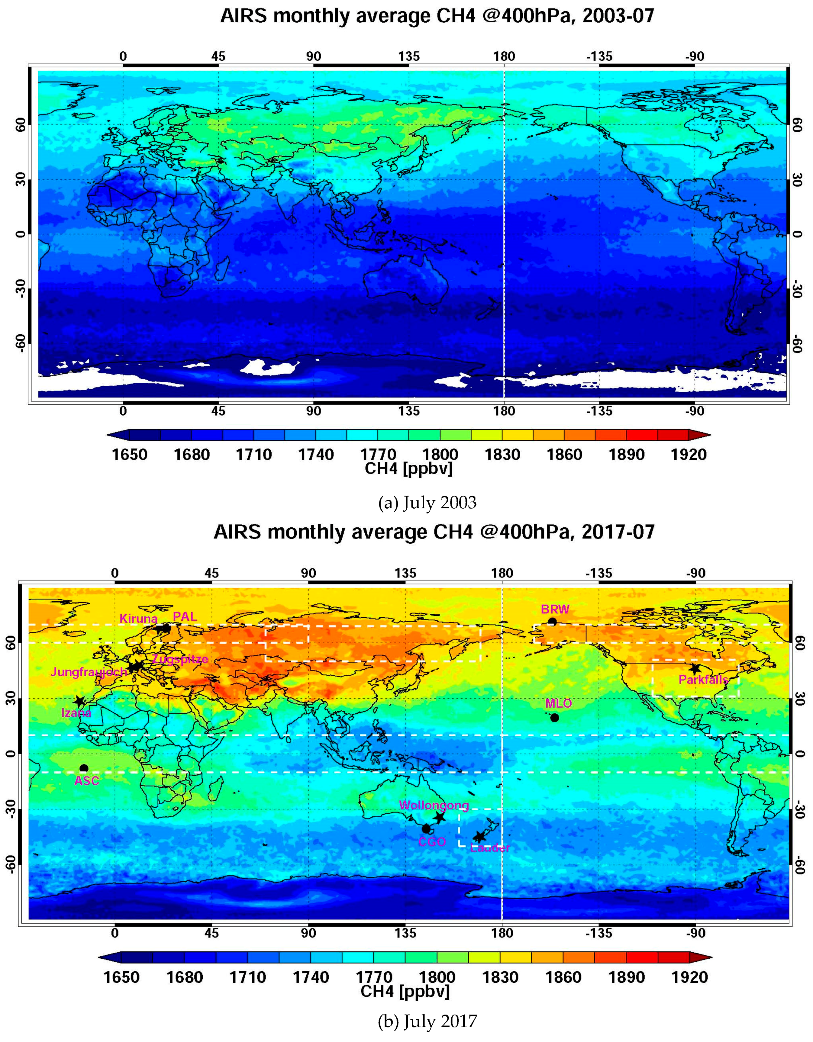
As a thermal infrared sounder that has been very stable since its launch and of which is still under operation, AIRS on the EOS/Aqua satellite was launched in polar orbit (13:30 local standard time, ascending node) in May 2002. It has 2378 channels covering 649–1136, 1217–1613, and 2169–2674 cm−1 at high spectral resolution (λ/∆λ = 1200) [8] and the noise in the equivalent change in temperature (Ne∆T) at a reference temperature of 250 K ranges from 0.14 K in the 4.2 μm in the lower tropospheric sounding wavelengths to 0.35 K in the 15 μm in the upper tropospheric sounding region. The spatial resolution of AIRS is 13.5 km at nadir and in a 24-hour period, AIRS nominally observes the complete globe twice. In order to retrieve CH4 in both clear and partially cloudy scenes, nine AIRS fields-of-views (FOVs) within the footprint of the Advanced Microwave Sounding Unit (AMSU) are used to derive a single cloud-cleared radiance spectrum in a field-of-regard (FOR), which is then used to retrieve profiles with a spatial resolution of approximately 45 km. The atmospheric temperature profiles, water vapor profiles, surface temperatures, and surface emissivity are required as inputs to simulate the clear radiances in the CH4 absorption band, and these inputs are retrieved from AIRS using different channels. The differences between the computed radiances and the AIRS measured radiances for clear pixels or the derived cloud-cleared FOR radiances for partially cloudy pixels are used to derive the change of CH4 profiles. Then, 50–60 CH4 absorption channels near 7.66 µm band were selected for the retrievals. The AIRS retrieval algorithm is a sequential retrieval method with multiple steps in which the temperature and water vapor profiles were retrieved using its own sensitive channels in previous steps before CH4 retrieval, thus the quality of the CH4 retrievals strongly depends on the AIRS retrieved temperature and moisture profiles as well as surface temperature and emissivity products. More detail of CH4 retrievals in its most recent version, i.e. version six (V6), can be found in Xiong et al. [28]. The most sensitivity of AIRS to atmospheric CH4 is in the mid–upper troposphere. The mid–upper tropospheric CH4 dataset (AIRX3STD) retrieved using both AIRS and AMSU (Advanced Microwave Sounding Unit) observations are used in this study. Validation of the latest operational CH4 product (AIRS version six) was made by comparing with aircraft data [28], which demonstrates that its RMS error (RMSE) is mostly less than 1.5%. Due to the failure of some AMSU channel, only the AIRS CH4 data in the period from August 2002 to December of 2016 were used. From the global monthly averaged map of CH4 at 400 hPa level in July 2003 and 2017 (Figure 1), we can clearly see the significant increase of CH4 globally and the increase is up to 100 ppbv in most regions.
For comparison of CH4 trends among the three measurements, a few regions of AIRS measurements were selected. Table 1 lists the latitudes and longitudes of the regions used. Daily CH4 concentrations at the 400 hPa level are extracted from AIRS CH4 profile products in each of these regions which are then used to calculate the regional average.
2.2. Column-Averaged CH4 Measurements from the TCCON and NDACC Network
The Total Carbon Column Observing Network (TCCON) is designed to retrieve precise and accurate column abundances of CO2, CH4, N2O, and CO, as well as HF, H2O, and HDO from near infrared solar absorption spectra measured by ground-based Fourier Transform Spectrometers (FTS). The TCCON was established in 2004 [29] and currently there are 21 sites that are operational. The TCCON processed scheme is designed to minimize algorithmic biases between sites. To this end, a common and open source software package was used for data processing and analysis. The retrieval approach was carried out by the GFIT nonlinear least-squares fitting algorithm [30,31], which minimizes the residue between the recorded spectra and forward model calculation. It is estimated to achieve a precision of ~ 0.25% for CO2 global monthly means [29,32] and ~ 0.5% for CH4 tropospheric volume mixing ratios [33]. More information and data are available from https://tccon-wiki.caltech.edu/. TCCON CH4 measurements acquired before and after AIRS pass time of ascending mode are selected to calculate the monthly mean value. Since the start date was not the same for different ground stations, we only selected two ground stations that have a longer period of measurements: one is Parkfalls located at the mid-latitude regions in the northern hemisphere [34,35,36] and the other is Lauder located in the mid-latitude of the southern hemisphere [37,38].
The international Network for the Detection of Atmosphere Composition Change (NDACC) is a major component of the international atmospheric research effort. The NDACC is composed of a set of globally distributed, high-quality, remote-sensing research stations for observing and understanding the physical and chemical state of the stratosphere and upper troposphere. Ground-based FTIRs from NDACC provide consistent, long-term measurements of the CH4 column averaged volume-mixing ratio (Xch4). We used Xch4 from seven sites, which are listed in Table 2 to form the trend analysis.
2.3. Surface CH4 Measurements from the NOAA/ESRL/GMD Network
The NOAA Global Monitoring Division (GMD) is a world leader in producing the regional to global-scale, long-term measurement records which allow quantification of the most important drivers of climate change. Global monitoring of greenhouse gases has been part of NOAA’s mission for over 50 years. NOAA/ESRL/GMD is the World Meteorological Organization (WMO), Global Atmosphere Watch (GAW) Central Calibration Laboratory (CCL) for CO2, CH4, N2O, SF6, and CO. The methane WMO scale was expanded to cover the nominal range 300 to 2600 ppbv based on the 16 original primary standards prepared in 1991–1995 [39]. The NOAA/ESRL/GMD network includes a cooperative program for the carbon gases providing air samples from more than 70 global air sites. Since these ground measurements provide the most accurate measurements of CH4, for comparison, datasets from ground-based in situ measurements of CH4 in Barrow, Alaska (BRW) and Mauna Loa (MLO) were used for analysis. Another dataset from NOAA sampling network at Cape Grim, Tasmania (CGO) was also used for analyzing the trend in the Southern Hemisphere. These datasets are from ftp://aftp.cmdl.noaa.gov/data/trace_gases/CH4/flask/surface [40]. For further investigation of the surface CH4 trend from the northern hemisphere to the southern hemisphere, another eight ground stations from NOAA/GMD were also used for analysis. Table 3 lists the stations that were used in this study.
2.4. EEMD Method for Trend Analysis
Ensemble Empirical Mode Decomposition (EEMD) is used to analyze the changing trend. EEMD is based on EMD [41,42], an adaptive time–frequency data analysis method that has been proved to be quite versatile in a broad range of applications for extracting signals from data generated in noisy nonlinear and nonstationary processes (see, e.g., [43,44]).
In EMD, the data x(t) are decomposed in terms of “intrinsic mode functions” (IMFs) Cj, and a residual component Rn, i.e.,
In Equation (1), the residual component, Rn, could be a constant, a monotonic function, or a function that contains only a single extreme from which no more oscillatory IMFs can be extracted. The total number of IMFs of a data set is close to log2N [43,44], with N being the number of total data points. Different from many traditional decomposition methods, including the Fourier Transform and wavelet decomposition methods, EMD does not utilize a priori determined basis functions which may faithfully represent the characteristics of a time series in some segments, however not in other segments of a non-stationary time series. EEMD improves the stability of EMD when the extreme locations and values of analyzed data are changed by noise. More detail about EMD and EEMD can be found in Huang et al. and Wu et al. [43,44,45].
Temporal evolution of observables related to complex and not fully understood systems in nature is not a priori known. Using the EEMD derived trend of the obtained CH4 concentration time series improves the non-physical choice of simple linear dependence in a completely new and logically consistent way [44]. Wu et al. [45] has made comparison of global-mean surface temperature trends derived using EEMD and a traditionally piece-wise linear fitting approach, respectively. The featured multi-decadal variability from the linear fitted trend cannot describe the secular warming, while the warming rate of the EEMD trend is changing gradually, which provides a chance to diagnose the warming rate changes of the secular trend. The uncertainty of the trend in the EEMD method is determined using a Monte Carlo approach rather than using an arbitrary disturbance such as white-noise. The details of this method can be found in the appendix of Wu et al. [45]. For any time series, its secular trend is supposed to be slowly varying and containing some noise.
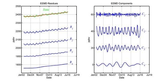
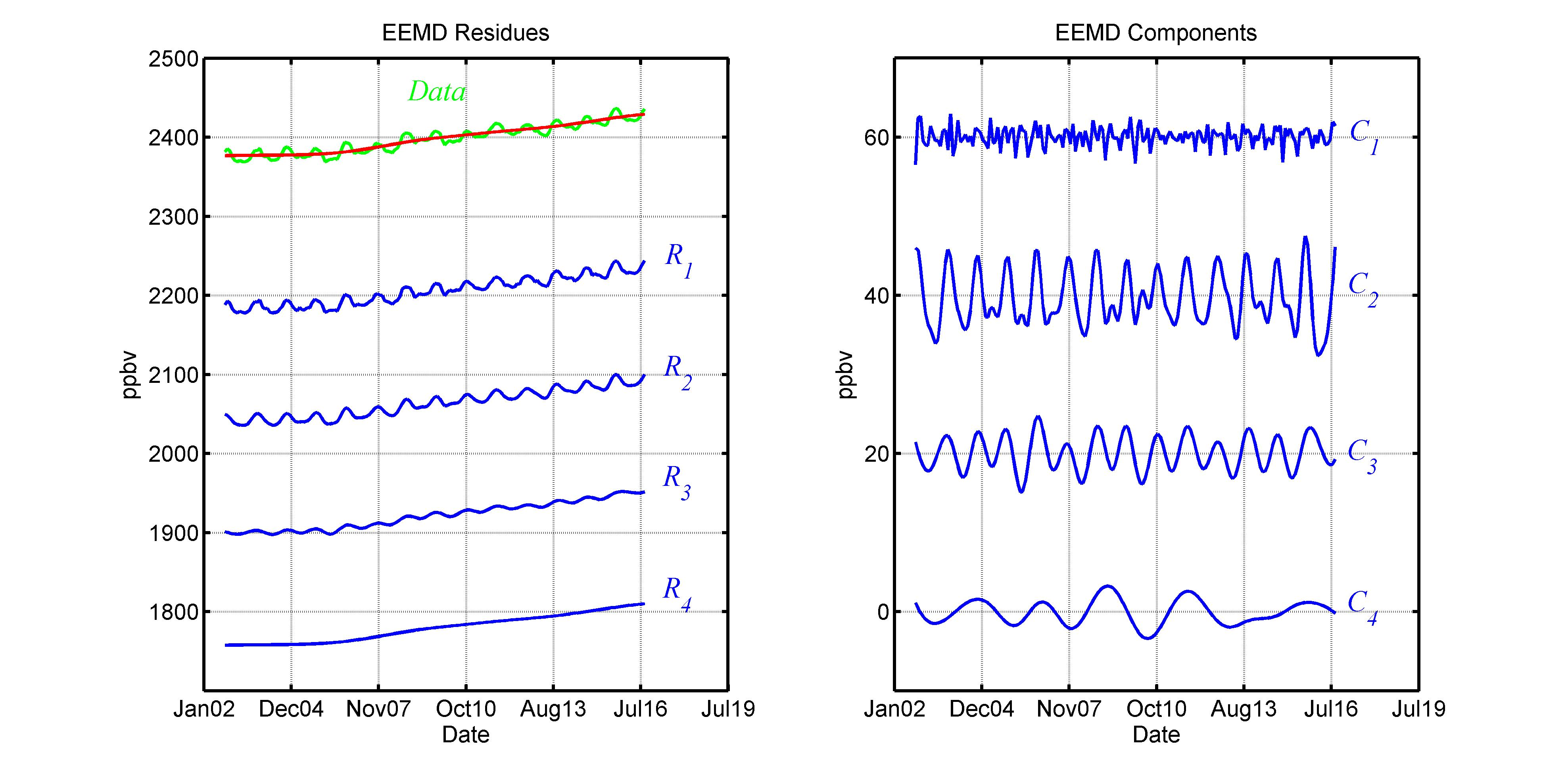
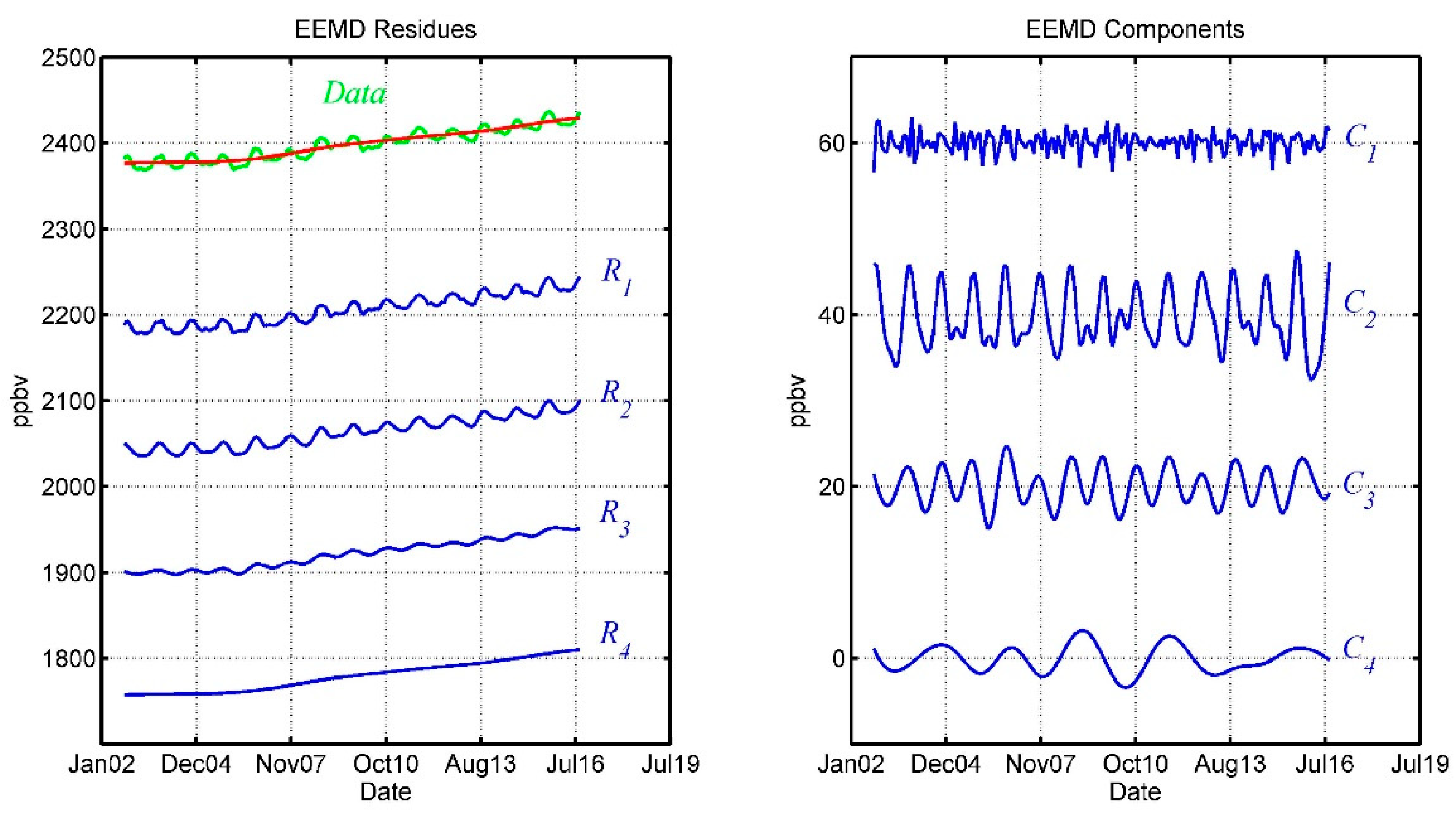
As an example, to illustrate the EEMD used in this paper, Figure 2 shows AIRS time series of regional mean CH4 at 400 hPa over Tropics and the EEMD decomposition results. The left panel of Figure 2 presents the residual components of decomposition. For a better view, Ri is plotted by adding (4 − i) × 142 (i = 1, 2, 3, 4); the original data (green line) and the final residua R4 (red line) are plotted by adding (4 × 142 + 50). The right panel shows the IMFs of decomposition and, similarly, Ci is plotted by adding (4 − i) × 20 (i = 1, 2, 3, 4). It is found that the use of four IMFs is good enough to characterize the variation. The total number of IMFs, four, is close to the estimated number log2N in Equation 1, where N ≈14.1 years using AIRS data from August 30, 2002 to September 24, 2016. IMFs C1, C2, C3, and C4 represent the CH4 variations with frequencies from high to low. The amplitudes of IMFs represent the strength of CH4 variation. C1 shows a fast oscillation yet low amplitude. C2 and C3 show much stronger oscillations and these two components can reflect the seasonal behavior of CH4. So, we will combine C2 and C3 decomposed from three measurements to clearly present the seasonal behavior of CH4 at different altitudes in Section 3.1. After three IMFS were extracted, C4 with the lowest oscillation frequency contain little information about CH4 variation. The final residual R4, represents the CH4 trend from EEMD analysis. R4 showed a rapid increase of CH4 since 2007 and an even higher increase in later 2013, as observed from surface measurement. The annual increase rates are obtained as the derivative of R4 with time.
To further test EEMD used for trend analysis, data from six NDACC stations were analyzed using the EEMD decomposition. For each station, 10 years series of total column CH4 (XCH4) since 2005 were decomposed to get the residual R4. The CH4 annual increase rates of these six stations were derived from R4 and the relative annual change percent was calculated referring to the monthly average in January 2005. Table 3 shows the relative changes of six stations and a comparison to those from Bader et al. [4]. We can see that the annual increases in all of these sites from this analysis using the EEMD method agrees quite well with those from Bader et al. [4] within the uncertainty range. One more advantage of the EEMD analysis is that we can derive the monthly rate of CH4 increase as a function of time, from which we can get more information of the CH4 change with time, making this research unique as compared to previous analysis.
3. Results and Discussion
3.1. Comparison of the Annual Increase Rates from Three Measurements
To be more concise for comparison, hereafter we will just plot the original data, four IMFs, and the residual R4 in a single axis. Since all of these data are of different scales, plots will be made omitting the label of the y-axis. To investigate the difference of CH4 variations between the mid–upper tropospheric (MUT) and surface, EEMD decomposition of AIRS CH4 over the Alaska region at 400 hPa level was conducted. The IMFs and final residual R4 are presented at the left column of Figure 3. Also, the similar decompositions of surface CH4 from BRW/NOAA station located near Alaska are shown in the right column for comparison. We combine C2 and C3 together to show a clearer seasonal cycle. According to Figure 3, it is evident that the IMFs amplitudes of surface CH4 (BRW/NOAA) are larger than those from the AIRS region mean. This means that surface CH4 has stronger seasonal variations. Besides, the residual R4 from two data sets both show a rapid increase since 2007, however the surface CH4 has a much larger increase rate. The residue R4 from BRW/NOAA measurement also shows a pronounced rapid increase since later in 2013, while the residue R4 from AIRS shows an almost linear increase.
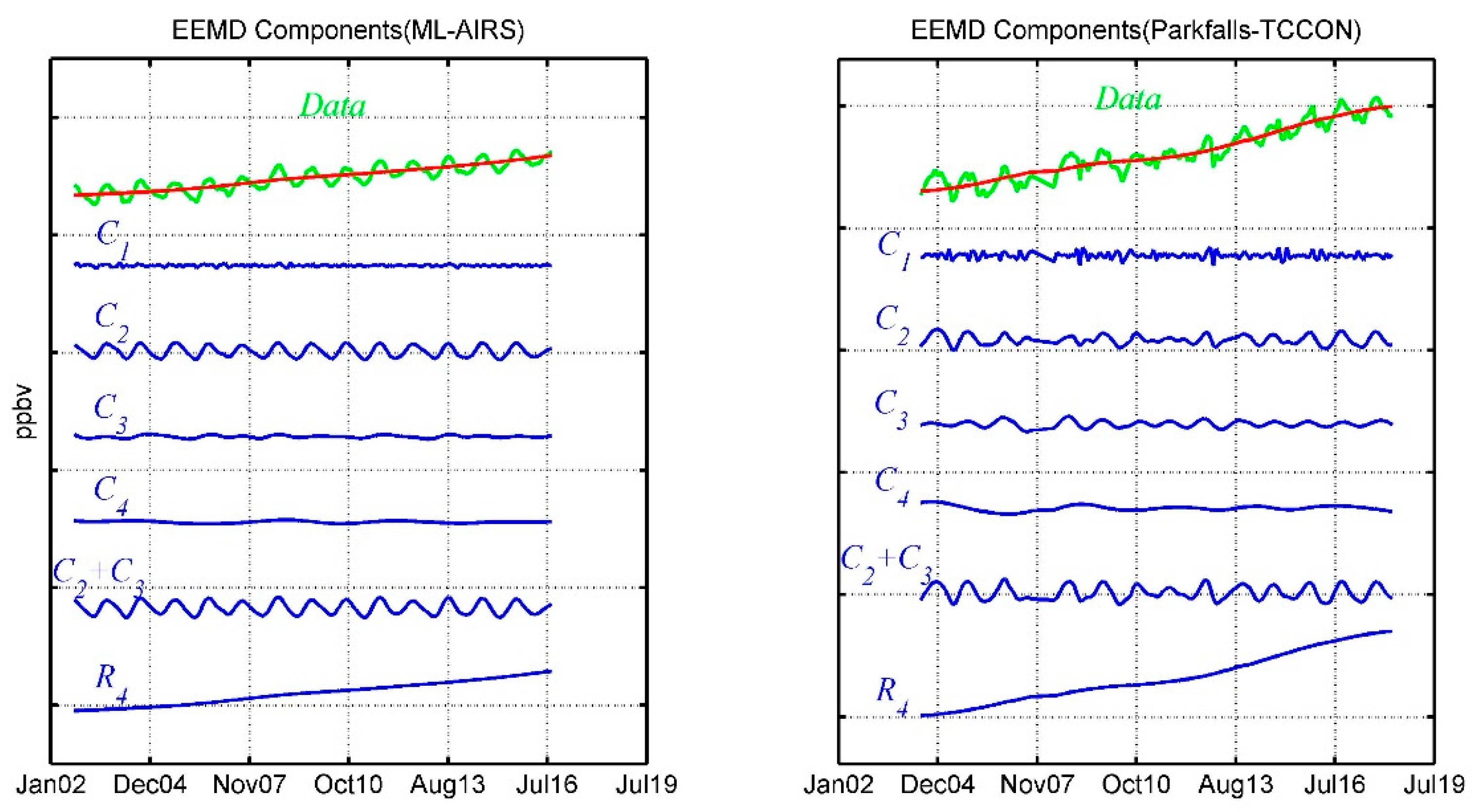
We also make comparison between MUT and total column-average CH4 (Xch4) measurements. EEMD decompositions of AIRS CH4 at 400 hPa level over the Mid-latitude region and XCH4 from Parkfalls/TCCON site located in the Mid-latitude region are presented in Figure 4. Comparing the combinations of (C2 + C3), we can find a very similar seasonal cycle with almost the same variations from these two data sets. The residual R4 from both data sets also shows a rapid increase since 2007. Since observations from ground FTIR are more sensitive to surface emission than AIRS, R4 from total column-average CH4 at Parkfalls/TCCON shows much larger increase rates than AIRS CH4, especially after later 2013. This is consistent with the comparison between AK-AIRS and BRW-NOAA.
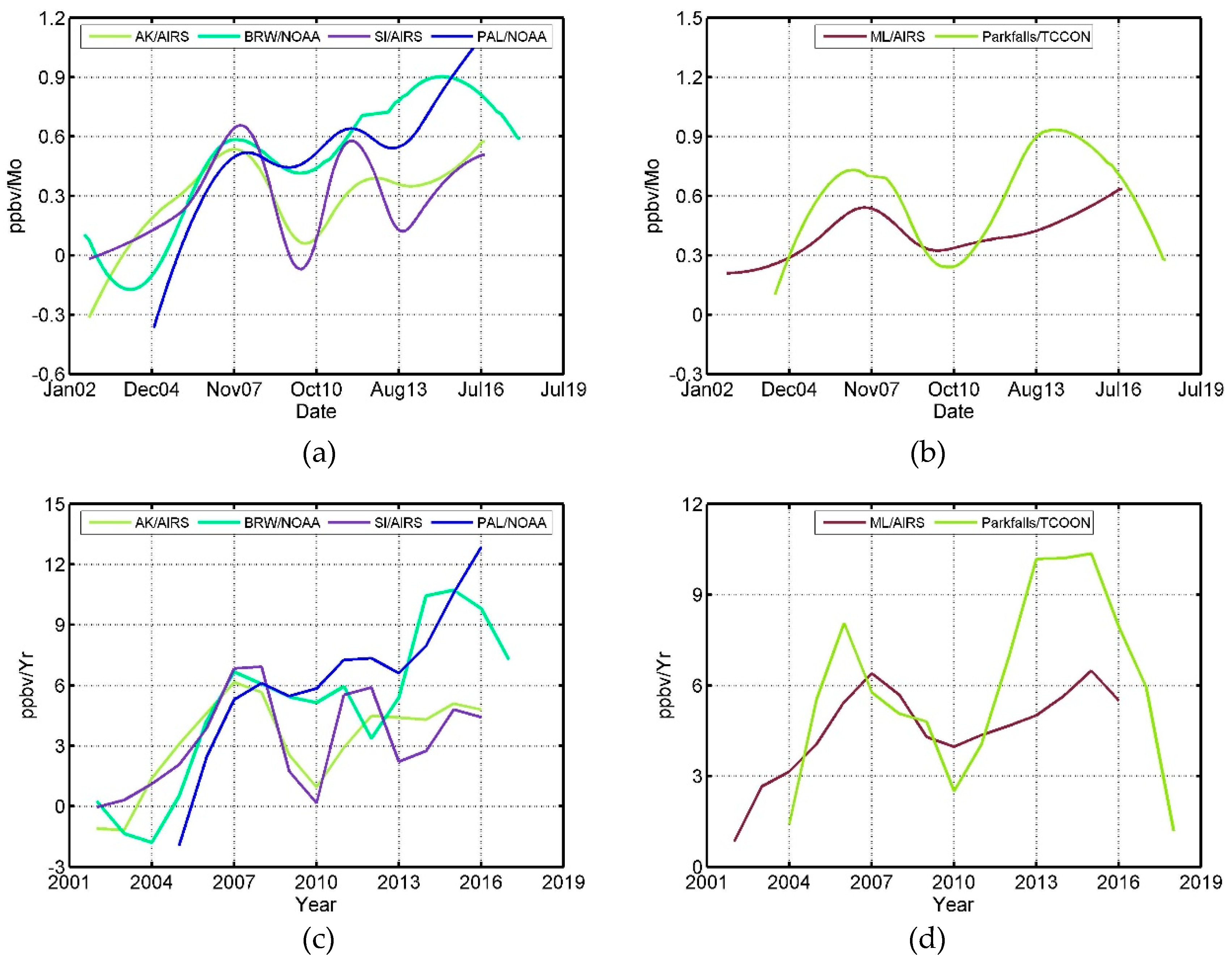
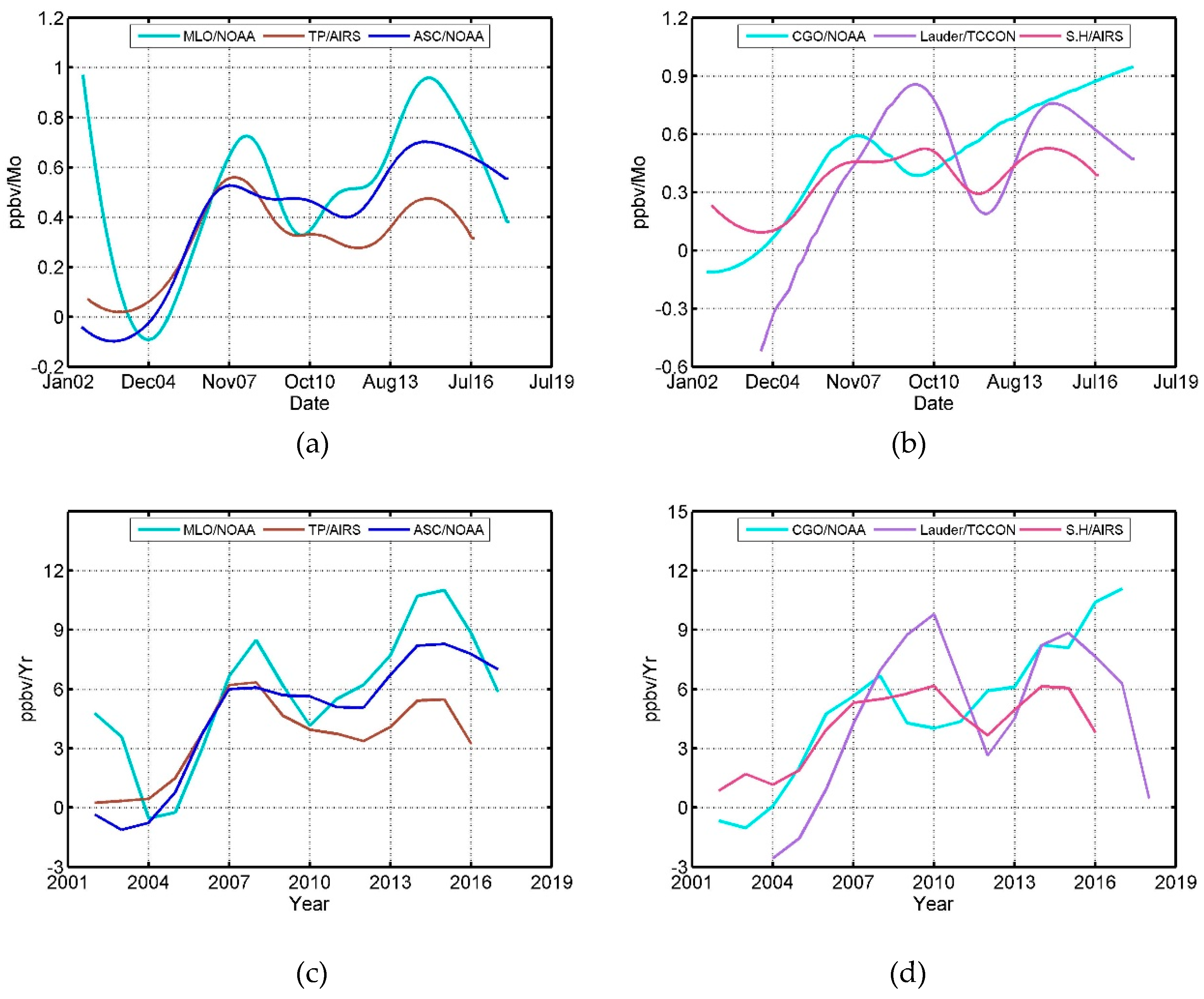
To make further comparison for the three different data sets, we quantify the monthly increase rates from the derivation of EEMD-decomposed residual R4 with respect to time. The annual increase rates are also calculated by integration of monthly rates. Figure 5 shows the comparison of CH4 increase rates derived from AIRS and the ground-based stations in the northern hemisphere and Figure 6 shows the similar comparison in the tropics and southern hemisphere. In the northern hemisphere, we find that the three measurements agree well and capture the increase around 2007. The maximum of the column-average Xch4 (Parkfalls/TCCON) occurred one year earlier than in the Arctic (Figure 5b,d). The second annual increase peaks of both Xch4 and MUT CH4 in the mid-latitude occurred in 2015. CH4 in the MBL and in the MUT have similar pace when the maximum occurred (Figure 5a,c), however there is a slight phase shift (delay) of about three months over Siberia (February 2008) compared to Alaska (November 2007) and the maximum of MUT CH4 over the Mid-latitude region occurred even earlier (August 2007). Things are different about the second increase peaks between Alaska and Siberia. Increase rates of both MUT and MBL CH4 in Alaska reached the maximum in 2015, however the rate of MBL CH4 in Siberia (PAL/NOAA) kept rising after 2015. During the period from 2009 to 2011, there are obvious dips in increase rates for the MUT, MBL, and total column CH4 in the mid–high latitude regions. All the annual increase rates reach the minimum at year 2010. In the tropics and southern hemisphere (Figure 6), the phases of these three measurements agree quite well, however there is a delay of phase from the northern hemisphere to the tropics and a further delay in the high southern hemisphere. The shift of phases from MBL to MUT and from the northern hemisphere to southern hemisphere can be explained by the transport of CH4 from the surface to the upper troposphere and transport from the northern hemisphere. The occurrence of the maxima of the column-average of CH4 and AIRS CH4 earlier than in other regions may indicate that the driver of CH4 increase in 2007 is from the mid-latitude regions. This finding may echo a recent study by Schwietzke et al. [46] that found the emission of CH4 from industrial sources is larger than previous estimates. The study by Bader et al. [4] also pointed out that anthropogenic emissions such as coal mining and gas and oil transport and exploration, which were mainly emitted in the Northern Hemisphere, had played a major role in the increase of atmospheric methane observed since 2005.
Vrekoussis et al. [47] pointed out that the economic crisis from 2008 resulted in a reduction of anthropogenic activities emitting gaseous pollutants, such as CO, NO2, and SO2. The strong correlation between the measured pollutants and several indicators of economic activity (Gross Domestic Product, Industrial Production Index, and Oil Consumption) may corroborate that economic recession has resulted in a reduction of air pollutants. Zhang et al. [48] also reported the reduction of measured Volatile Organic Compounds (VOCs) in 2008 after the financial crisis compared to that in 2007, which is due to the reduced emission from industries that were hard-hit by the financial crisis. Amann et al. estimated the GHG mitigation potentials and costs based on the simulation from the GAINS (Greenhouse gas-Air Pollution Interactions and Synergies) model [49]. Two economic projections, WEO2008 and WEO2009, which were developed before and after the 2008 economic crisis, were adopted to evaluate the impact of the economic crisis. Simulations indicate that WEO 2009 projection of economic development led to 8% less GHG emissions for 2020 compared to WEO 2008. So, it is likely that the financial crisis in 2008 led to the slow-down of the CH4 increase rate until 2010. Bergamaschi et al. [50] also pointed out that a large increase in anthropogenic CH4 emissions first occured from 2006 and beyond.
It is noteworthy that the increase rates reversed later and reached another peak in 2014 which was even larger than in 2007. In this cycle in 2014, the peak in mid-latitude from TCCON took the lead and the peaks in the tropics and southern hemisphere still lag behind the northern hemisphere. This difference suggests that the emissions from human activities in the mid-latitude is likely playing a major role, which is also echoed from the slow-down of CH4 in 2009–2010 corresponding to the financial crisis in 2008.
3.2. Trend of Zonal Mean CH4 in the Mid–Upper Troposphere
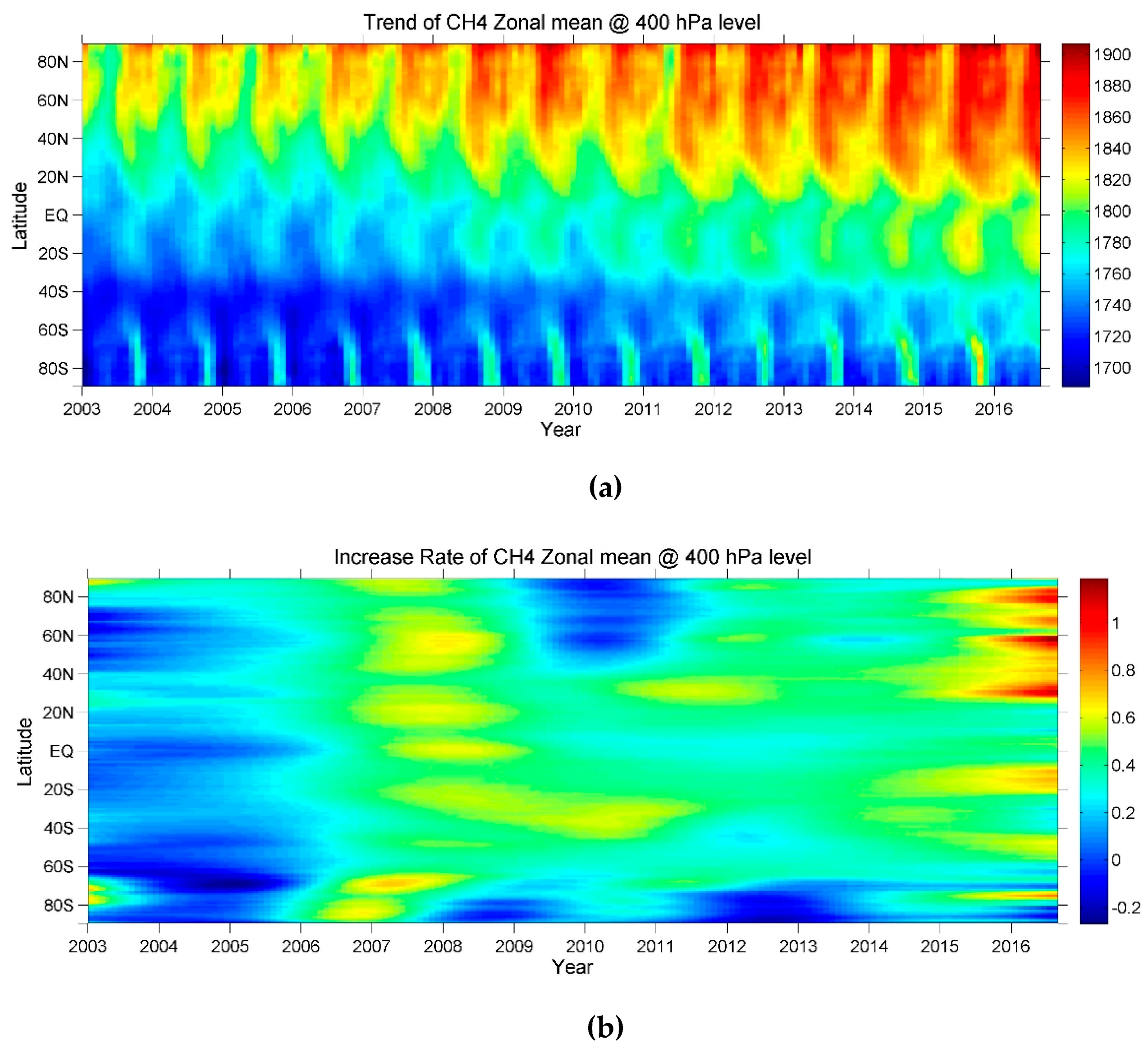
To have a better picture of the global CH4 variation with regards to time, EEMD decomposition can be applied to AIRS zonal mean CH4 at 400 hPa level for trend analysis. Global zonal mean CH4 is calculated at monthly scale and its time series from 2003 to 2016 is shown in Figure 7a. It is clearly shown that the mean CH4 is much higher in the northern hemisphere than in the southern hemisphere. In the northern hemisphere, the zonal mean CH4 shows strongly seasonal behavior as the maximum appears in summer and the minimum appears in spring. The overall increase trend in the northern hemisphere is larger than in the southern hemisphere and the gradient of the merge line between the northern and southern hemisphere has a tendency towards the southern. The corresponding increase rates of monthly zonal mean are derived from the EEMD decomposition analysis and are presented in Figure 7b. According to the increase rates, it is clearly shown that there is a large increase from the northern to the southern hemisphere around 2007 and there is evident phase delay of increase rates between the southern and the northern hemisphere. In the years afterwards, the increase rates over the tropics are slightly smaller than both the northern and southern subtropics regions. We can also find the slowing down of CH4 increase around 2010 over the mid-to-high latitude region. The second rapid increase period starts around 2014. The increase rates reached to extremely high values over the subtropics to the high latitude region in the northern hemisphere and over the subtropics in the southern hemisphere, which are even larger than those in 2007. One small yet interesting feature is from 2009 to 2016 as the increase rates of MUT-CH4 over the tropics are slightly smaller than that over the northern and southern subtropics regions and the reasons are unknown.
In addition to the impact by emission sources, the CH4 trend is also impacted by changes in the atmospheric CH4 loss and soil uptake. Dalsøren et al. found that from 2000–2010, the modelled tropospheric OH column increased by 10–20% over China and India, and many model studies demonstrated a decrease in CH4 lifetime due to an increase in global OH concentrations in the recent decades [51]. However, as discussed by Dalsøren et al., there is a missing consensus on OH trends among different studies. Some more studies also show a strong influence of El Niño–Southern Oscillation (ENSO) events on CH4. Corbett et al. [52] also show the modulation of mid-tropospheric CH4 by El Niño.
4. Conclusions
An advanced statistical analysis method, EEMD method, was used for the first time to analyze the trends of atmospheric CH4 from 2003 to 2016 from three different measurements’ datasets. The agreement of the annual increases in a few sites from this EEMD analysis with those from Bader et al. [4] proved the capability to use the EEMD method to analyze the CH4 trends. Even more, by using EEMD analysis, we can derive the monthly increase rates of CH4 which gives us more information about the CH4 change with time.
Using this EEMD method, the monthly and annual increase rates of CH4 in the marine boundary layer and the mid–upper troposphere, as well as the column average, were derived and compared in this study. Regardless of the difference in the uncertainties from these three measurements and their sensitivities to CH4 variation in different altitudes, the analysis of the CH4 trend and monthly/annual rates using three data sets in the northern hemisphere, tropics, and the southern hemisphere in this study demonstrated:
- (1)
- One common feature among these three measurements is that they have good agreement in capturing the abrupt increase of CH4 in 2007. The increase rates of CH4 in the MUT, as observed by AIRS, are overall smaller than CH4 in MBL and the column-average CH4.
- (2)
- During 2009–2011, there was a dip in the increase rate for CH4 in MBL and the MUT-CH4 increase rate was near zero in the mid–high northern latitude regions. The increase of the column-average CH4, also reached a minimum correspondingly. Such a slow-down of increase rate might echo other studies that pointed out that the emission of CH4 from industrial sources plays a large role in recent CH4 increase as such a slow-down might be linked with the reduced industrial emission due to the financial crisis in 2008.
- (3)
- Increase rates reached another peak since 2014 which is even larger than in 2007, so a continual monitoring of the trends of CH4 using both ground-based and space-borne measurement is important for climate change study.
Author Contributions
Conceptualization, M.Z. and X.X.; Data curation, M.Z., S.L. and Y.Z.; Formal analysis, M.Z. and X.X.; Funding acquisition, M.Z.; Investigation, X.X.; Methodology, Z.W.; Software, Z.W.; Supervision, X.X. and L.C.; Visualization, M.Z. and X.X.; Writing – original draft, M.Z. and X.X.; Writing – review & editing, M.Z. and X.X.
Funding
This research was funded by the National Natural Science Foundation of China, grant number 41771390, Program of Remote Sensing with high spatial resolution, 32-Y20A17-9001-15-17-2, and Project for data application of FY3 meteorological satellite.
Acknowledgments
We are grateful to the NOAA/ESRL/GMD for providing the ground-based measurements of CH4 and the data used is from NOAA ESRL Global Monitoring Division, Carbon Cycle and Greenhouse Gases group, 325 Broadway R/CSD, Boulder, CO 80305 (http://esrl.noaa.gov/gmd/ccgg/). TCCON measurements from Park Falls were funded by NASA grants NNX14AI60G, NNX11AG01G, NAG5-12247, NNG05-GD07G, and NASA Orbiting Carbon Observatory Program. We are grateful to Jeff Ayers for technical support in Park Falls. The Lauder TCCON measurements were core-funded by NIWA through New Zealand’s Ministry of Business, Innovation, and Employment. The TCCON CH4 data is downloaded from https://tccon-wiki.caltech.edu/. The XCH4 data from NDACC that was used in this publication were obtained as part of the Network for the Detection of Atmospheric Composition Change (NDACC) and are publicly available (see http://www.ndacc.org).
Conflicts of Interest
The authors declare no conflict of interest.
References
- Stocker, T.F.; Qin, D.; Plattner, G.-K.; Tignor, M.; Allen, S.K.; Boschung, J.; Nauels, A.; Xia, Y.; Bex, V.; Midgley, P.M. IPCC, Climate Change 2013: The Physical Science Basis. Contribution of Working Group I to the Fifth Assessment Report of the Intergovernmental Panel on Climate Change; Cambridge University Press: Cambridge, UK; New York, NY, USA, 2013. [Google Scholar]
- Dlugokencky, E.J.; Crotwell, A.M.; Bruhwiler, L.; Masarie, K.A.; Lang, P.M.; White, J.W.C.; Michel, S.E. The Dominant Role of Tropical Wetlands in Dedacal-Scale Changes in the Global Methane Budget. Abstract A33C-0162. Presented at 2015 Fall Meeting, AGU, San Francisco, CA, USA, 14–18 December 2015. [Google Scholar]
- Dlugokencky, E.J.; Bruhwiler, L.; White, J.W.C.; Emmons, L.K.; Novelli, P.C.; Montzka, S.A.; Masarie, K.A.; Lang, P.M.; Crotwell, A.M.; Miller, J.B.; et al. Observational constraints on recent increases in the atmospheric CH4 burden. Geophys. Res. Lett. 2009, 36. [Google Scholar] [CrossRef]
- Bader, W.; Bovy, B.; Conway, S.; Strong, K.; Smale, D.; Turner, A.J.; Blumenstock, T.; Boone, C.; Collaud Coen, M.; Coulon, A.; et al. The recent increase of atmospheric methane from 10 years of ground-based NDACC FTIR observations since 2005. Atmos. Chem. Phys. 2017, 17, 2255–2277. [Google Scholar] [CrossRef] [Green Version]
- Nisbet, E.G.; Dlugokencky, E.J.; Manning, M.R.; Lowry, D.; Fisher, R.E.; France, J.L.; Michel, S.E.; Miller, J.B.; White, J.W.C.; Vaughn, B.; et al. Rising atmospheric methane: 2007–2014 growth and isotopic shift. Glob. Biogeochem. Cycles 2016, 30, 1356–1370. [Google Scholar] [CrossRef]
- Warneke, T.; Yang, Z.; Olsen, S.; Körner, S.; Notholt, J.; Toon, G.C.; Velazco, V.; Schulz, A.; Schrems, O. Seasonal and latitudinal variations of column averaged volume-mixing ratios of atmospheric CO2. Geophys. Res. Lett. 2005, 32. [Google Scholar] [CrossRef]
- Sussmann, R.; Stremme, W.; Buchwitz, M.; de Beek, R. Validation of ENVISAT/SCIAMACHY columnar methane by solar FTIR spectrometry at the Ground-Truthing Station Zugspitze. Atmos. Chem. Phys. 2005, 5, 2419–2429. [Google Scholar] [CrossRef] [Green Version]
- Sussmann, R.; Rettinger, M.; Borsdorff, T. On seasonality of the indirect greenhouse gas CO above Europe: An altitude-resolved picture from long-term FTIR measurements. In Proceedings of the EGU General Assembly Conference Abstracts, Vienna, Austria, 2–7 May 2010; p. 15406. [Google Scholar]
- Tans, P.P. The Atmospheric Buildup Rate for Carbon is Based on Measurements of CO2 at Mauna Loa Obtained by the NOAA Earth System Research Laboratory. 2009. Available online: www.esrl.noaa.gov/gmd/ccgg/trends/ (accessed on 5 October 2015).
- Aumann, H.H.; Chahine, M.T.; Gautier, C.; Goldberg, M.D.; Kalnay, E.; McMillin, L.M.; Revercomb, H.; Rosenkranz, P.W.; Smith, W.L.; Staelin, D.H.; et al. AIRS/AMSU/HSB on the Aqua mission: Design, science objectives, data products, and processing systems. IEEE Trans. Geosci. Remote Sens. 2003, 41, 253–264. [Google Scholar] [CrossRef]
- Xiong, X.; Barnet, C.; Maddy, E.; Sweeney, C.; Liu, X.; Zhou, L.; Goldberg, M. Characterization and validation of methane products from the Atmospheric Infrared Sounder (AIRS). J. Geophys. Res. 2008, 113, G00A01. [Google Scholar] [CrossRef]
- Xiong, X.; Barnet, C.; Maddy, E.; Wei, J.; Liu, X.; Pagano, T.S. Seven Years’ Observation of Mid-Upper Tropospheric Methane from Atmospheric Infrared Sounder. Remote Sens. 2010, 2, 2509–2530. [Google Scholar] [CrossRef] [Green Version]
- Xiong, X.; Barnet, C.D.; Zhuang, Q.; Machida, T.; Sweeney, C.; Patra, P.K. Mid-upper tropospheric methane in the high Northern Hemisphere: Spaceborne observations by AIRS, aircraft measurements, and model simulations. J. Geophys. Res. Atmos. 2010, 115. [Google Scholar] [CrossRef] [Green Version]
- Payne, V.H.; Clough, S.A.; Shephard, M.W.; Nassar, R.; Logan, J.A. Information-centered representation of retrievals with limited degrees of freedom for signal: Application to methane from the Tropospheric Emission Spectrometer. J. Geophys. Res. Atmos. 2009, 114. [Google Scholar] [CrossRef] [Green Version]
- Wecht, K.J.; Jacob, D.J.; Wofsy, S.C.; Kort, E.A.; Worden, J.R.; Kulawik, S.S.; Henze, D.K.; Kopacz, M.; Payne, V.H. Validation of TES methane with HIPPO aircraft observations: Implications for inverse modeling of methane sources. Atmos. Chem. Phys. 2012, 12, 1823–1832. [Google Scholar] [CrossRef]
- Worden, J.; Kulawik, S.; Frankenberg, C.; Payne, V.; Bowman, K.; Cady-Peirara, K.; Wecht, K.; Lee, J.E.; Noone, D. Profiles of CH4, HDO, H2O, and N2O with improved lower tropospheric vertical resolution from Aura TES radiances. Atmos. Meas. Tech. 2012, 5, 397–411. [Google Scholar] [CrossRef]
- Xiong, X.; Barnet, C.; Maddy, E.S.; Gambacorta, A.; King, T.S.; Wofsy, S.C. Mid-upper tropospheric methane retrieval from IASI and its validation. Atmos. Meas. Tech. 2013, 6, 2255–2265. [Google Scholar] [CrossRef] [Green Version]
- Crevoisier, C.; Nobileau, D.; Fiore, A.M.; Armante, R.; Chédin, A.; Scott, N.A. Tropospheric methane in the tropics-first year from IASI hyperspectral infrared observations. Atmos. Chem. Phys. 2009, 9, 6337–6350. [Google Scholar] [CrossRef]
- Crevoisier, C.; Nobileau, D.; Armante, R.; Crépeau, L.; Machida, T.; Sawa, Y.; Matsueda, H.; Schuck, T.; Thonat, T.; Pernin, J.; et al. The 2007–2011 evolution of tropical methane in the mid-troposphere as seen from space by MetOp-A/IASI. Atmos. Chem. Phys. 2013, 13, 4279–4289. [Google Scholar] [CrossRef] [Green Version]
- Razavi, A.; Clerbaux, C.; Wespes, C.; Clarisse, L.; Hurtmans, D.; Payan, S.; Camy-Peyret, C.; Coheur, P.F. Characterization of methane retrievals from the IASI space-borne sounder. Atmos. Chem. Phys. 2009, 9, 7889–7899. [Google Scholar] [CrossRef] [Green Version]
- Frankenberg, C.; Bergamaschi, P.; Butz, A.; Houweling, S.; Meirink, J.F.; Notholt, J.; Petersen, A.K.; Schrijver, H.; Warneke, T.; Aben, I. Tropical methane emissions: A revised view from SCIAMACHY onboard ENVISAT. Geophys. Res. Lett. 2008, 35. [Google Scholar] [CrossRef] [Green Version]
- Frankenberg, C.; Aben, I.; Bergamaschi, P.; Dlugokencky, E.J.; van Hees, R.; Houweling, S.; van der Meer, P.; Snel, R.; Tol, P. Global column-averaged methane mixing ratios from 2003 to 2009 as derived from SCIAMACHY: Trends and variability. J. Geophys. Res. Atmos. 2011, 116. [Google Scholar] [CrossRef] [Green Version]
- Parker, R.; Boesch, H.; Cogan, A.; Fraser, A.; Feng, L.; Palmer, P.I.; Messerschmidt, J.; Deutscher, N.; Griffith, D.W.T.; Notholt, J.; et al. Methane observations from the Greenhouse Gases Observing SATellite: Comparison to ground-based TCCON data and model calculations. Geophys. Res. Lett. 2011, 38. [Google Scholar] [CrossRef] [Green Version]
- Yokota, T.; Yoshida, Y.; Eguchi, N.; Ota, Y.; Tanaka, T.; Watanabe, H.; Maksyutov, S. Global Concentrations of CO2 and CH4 Retrieved from GOSAT: First Preliminary Results. SOLA 2009, 5, 160–163. [Google Scholar] [CrossRef]
- Schepers, D.; Guerlet, S.; Butz, A.; Landgraf, J.; Frankenberg, C.; Hasekamp, O.; Blavier, J.F.; Deutscher, N.M.; Griffith, D.W.T.; Hase, F.; et al. Methane retrievals from Greenhouse Gases Observing Satellite (GOSAT) shortwave infrared measurements: Performance comparison of proxy and physics retrieval algorithms. J. Geophys. Res. Atmos. 2012, 117. [Google Scholar] [CrossRef] [Green Version]
- Saitoh, N.; Touno, M.; Hayashida, S.; Imasu, R.; Shiomi, K.; Yokota, T.; Yoshida, Y.; Machida, T.; Matsueda, H.; Sawa, Y. Comparisons between XCH4 from GOSAT Shortwave and Thermal Infrared Spectra and Aircraft CH4 Measurements over Guam. SOLA 2012, 8, 145–149. [Google Scholar] [CrossRef]
- Kirschke, S.; Bousquet, P.; Ciais, P.; Saunois, M.; Canadell, J.G.; Dlugokencky, E.J.; Bergamaschi, P.; Bergmann, D.; Blake, D.R.; Bruhwiler, L.; et al. Three decades of global methane sources and sinks. Nat. Geosci. 2013, 6, 813. [Google Scholar] [CrossRef]
- Xiong, X.; Weng, F.; Liu, Q.; Olsen, E. Space-borne observation of methane from atmospheric infrared sounder version 6: Validation and implications for data analysis. Atmos. Meas. Tech. Discuss. 2015, 8563–8597. [Google Scholar] [CrossRef]
- Wunch, D.; Toon, G.C.; Wennberg, P.O.; Wofsy, S.C.; Stephens, B.B.; Fischer, M.L.; Uchino, O.; Abshire, J.B.; Bernath, P.; Biraud, S.C.; et al. Calibration of the Total Carbon Column Observing Network using aircraft profile data. Atmos. Meas. Tech. 2010, 3, 1351–1362. [Google Scholar] [CrossRef] [Green Version]
- Wunch, D.; Toon, G.C.; Blavier, J.-F.O.L.; Washenfelder, R.A.; Notholt, J.; Connor, B.J.; Griffith, D.W.T.; Sherlock, V.; Wennberg, P.O. The Total Carbon Column Observing Network. Philos. Trans. R. Soc. A Math. Phys. Eng. Sci. 2011, 369, 2087. [Google Scholar] [CrossRef]
- Sussmann, R.; Ostler, A.; Forster, F.; Rettinger, M.; Deutscher, N.M.; Griffith, D.W.T.; Hannigan, J.W.; Jones, N.; Patra, P.K. First intercalibration of column-averaged methane from the Total Carbon Column Observing Network and the Network for the Detection of Atmospheric Composition Change. Atmos. Meas. Tech. 2013, 6, 397–418. [Google Scholar] [CrossRef] [Green Version]
- Miller, C.E.; Crisp, D.; DeCola, P.L.; Olsen, S.C.; Randerson, J.T.; Michalak, A.M.; Alkhaled, A.; Rayner, P.; Jacob, D.J.; Suntharalingam, P.; et al. Precision requirements for space-based data. J. Geophys. Res. Atmos. 2007, 112. [Google Scholar] [CrossRef] [Green Version]
- Washenfelder, R.A.; Wennberg, P.O.; Toon, G.C. Tropospheric methane retrieved from ground-based near-IR solar absorption spectra. Geophys. Res. Lett. 2003, 30. [Google Scholar] [CrossRef] [Green Version]
- Washenfelder, R.A.; Toon, G.C.; Blavier, J.F.; Yang, Z.; Allen, N.T.; Wennberg, P.O.; Vay, S.A.; Matross, D.M.; Daube, B.C. Carbon dioxide column abundances at the Wisconsin Tall Tower site. J. Geophys. Res. Atmos. 2006, 111. [Google Scholar] [CrossRef] [Green Version]
- Wunch, D.; Wennberg, P.O.; Toon, G.C.; Keppel-Aleks, G.; Yavin, Y.G. Emissions of greenhouse gases from a North American megacity. Geophys. Res. Lett. 2009, 36. [Google Scholar] [CrossRef] [Green Version]
- Wennberg, P.O.; Roehl, C.; Wunch, D.; Toon, G.C.; Blavier, J.F.; Washenfelder, R.; Keppel-Aleks, G.; Allen, N.; Ayers, J. TCCON Data from Park Falls, Wisconsin, USA, Release GGG2014R0; CDIAC: Oak Ridge National Laboratory, Oak Ridge, TN, USA, 2014. [Google Scholar] [CrossRef]
- Sherlock, V.; Connor, B.; Robinson, J.; Shiona, H.; Smale, D.; Pollard, D. TCCON Data from Lauder, New Zealand, 120HR, Release GGG2014R0; CDIAC: Oak Ridge National Laboratory, Oak Ridge, TN, USA, 2014. [Google Scholar] [CrossRef]
- Sherlock, V.; Connor, B.; Robinson, J.; Shiona, H.; Smale, D.; Pollard, D. TCCON Data from Lauder, New Zealand, 125HR, Release GGG2014R0; CDIAC: Oak Ridge National Laboratory, Oak Ridge, TN, USA, 2014. [Google Scholar] [CrossRef]
- Dlugokencky, E.J.; Myers, R.C.; Lang, P.M.; Masarie, K.A.; Crotwell, A.M.; Thoning, K.W.; Hall, B.D.; Elkins, J.W.; Steele, L.P. Conversion of NOAA atmospheric dry air CH4 mole fractions to a gravimetrically prepared standard scale. J. Geophys. Res. 2005, 110. [Google Scholar] [CrossRef]
- ESRL; NOAA. GLOBALVIEW-CH4: Cooperative Atmospheric Data Integration Project—Methane; CD-ROM: Boulder, Colorado, 2009. [Google Scholar]
- Huang, N.E.; Shen, Z.; Long, S.R.; Wu, M.C.; Shih, H.H.; Zheng, Q.; Yen, N.-C.; Tung, C.C.; Liu, H.H. The empirical mode decomposition and the Hilbert spectrum for nonlinear and non-stationary time series analysis. Proc. R. Soc. Lond. Ser. A Math. Phys. Eng. Sci. 1998, 454, 903–955. [Google Scholar] [CrossRef]
- Huang, N.E.; Wu, Z. A review on Hilbert-Huang transform: Method and its applications to geophysical studies. Rev. Geophys. 2008, 46. [Google Scholar] [CrossRef] [Green Version]
- Wu, Z.; Huang, N.E. Ensemble empirical mode decomposition: A noise-assisted data analysis method. Adv. Adapt. Data Anal. 2009, 1, 1–41. [Google Scholar] [CrossRef]
- Wu, Z.; Huang, N.E.; Long, S.R.; Peng, C.-K. On the trend, detrending, and variability of nonlinear and nonstationary time series. Proc. Natl. Acad. Sci. USA 2007, 104, 14889–14894. [Google Scholar] [CrossRef] [Green Version]
- Wu, Z.; Huang, N.E.; Wallace, J.M.; Smoliak, B.V.; Chen, X. On the time-varying trend in global-mean surface temperature. Clim. Dyn. 2011, 37, 759–773. [Google Scholar] [CrossRef] [Green Version]
- Schwietzke, S.; Sherwood, O.A.; Bruhwiler, L.M.P.; Miller, J.B.; Etiope, G.; Dlugokencky, E.J.; Michel, S.E.; Arling, V.A.; Vaughn, B.H.; White, J.W.C.; et al. Upward revision of global fossil fuel methane emissions based on isotope database. Nature 2016, 538, 88. [Google Scholar] [CrossRef]
- Vrekoussis, M.; Richter, A.; Hilboll, A.; Burrows, J.P.; Gerasopoulos, E.; Lelieveld, J.; Barrie, L.; Zerefos, C.; Mihalopoulos, N. Economic crisis detected from space: Air quality observations over Athens/Greece. Geophys. Res. Lett. 2013, 40, 458–463. [Google Scholar] [CrossRef] [Green Version]
- Zhang, Y.L.; Wang, X.M.; Blake, D.R.; Li, L.F.; Zhang, Z.; Wang, S.Y.; Guo, H.; Lee, F.S.C.; Gao, B.; Chan, L.Y.; et al. Aromatic hydrocarbons as ozone precursors before and after outbreak of the 2008 financial crisis in the Pearl River Delta region, south China. J. Geophys. Res. Atmos. 2012, 117. [Google Scholar] [CrossRef] [Green Version]
- Markus, A.; Janusz, C.; Peter, R.; Fabian, W. The Impact of the Economic Crisis on GHG Mitigation Potentials and Costs in Annex I Countries, GAINS Report; International Institute for Applied Systems Analysis (IIASA): Laxenburg, Austria, 2009. [Google Scholar]
- Bergamaschi, P.; Houweling, S.; Segers, A.; Krol, M.; Frankenberg, C.; Scheepmaker, R.A.; Dlugokencky, E.; Wofsy, S.C.; Kort, E.A.; Sweeney, C.; et al. Atmospheric CH4 in the first decade of the 21st century: Inverse modeling analysis using SCIAMACHY satellite retrievals and NOAA surface measurements. J. Geophys. Res. Atmos. 2013, 118, 7350–7369. [Google Scholar] [CrossRef]
- Dalsøren, S.B.; Myhre, C.L.; Myhre, G.; Gomez-Pelaez, A.J.; Søvde, O.A.; Isaksen, I.S.A.; Weiss, R.F.; Harth, C.M. Atmospheric methane evolution the last 40 years. Atmos. Chem. Phys. 2016, 16, 3099–3126. [Google Scholar] [CrossRef] [Green Version]
- Corbett, A.; Jiang, X.; Xiong, X.; Kao, A.; Li, L. Modulation of midtropospheric methane by El Niño. Earth Space Sci. 2017, 4, 590–596. [Google Scholar] [CrossRef] [Green Version]
Figure 1.
Global monthly mean CH4 at 400 hPa level in July 2003 (a) and 2017 (b). Box areas indicated by dotted lines represent regions (listed in Table 1) used to calculate the Atmospheric Infrared Sounder (AIRS) average CH4. Ground-based stations with surface CH4 measurements used in this paper are marked with circles, as well as the ground sites with CH4 total column measurements (listed in Table 2, Section 2.2) marked with stars.

Figure 2.
Ensemble Empirical Mode Decomposition (EEMD) decomposition of the AIRS CH4 over the Tropics region. The left panel shows the original data (green line) and successive remainders (Rj) after an additional EEMD component (Cj) being extracted, i.e., Rj = Rj−1 − Cj for j > 1. The red line is the EEMD trend. In the right panel, each line represents an EEMD component (Cj) from high frequency to low frequency.

Figure 3.
EEMD decomposition of the AIRS CH4 over the Alaska region (left) and surface CH4 (right) from the Barrow/NOAA/GMD station. The original data (green line) together with the EEMD trend (red line), four EEMD components (Cj), and the remainder R4 are shown for each region.
Figure 3.
EEMD decomposition of the AIRS CH4 over the Alaska region (left) and surface CH4 (right) from the Barrow/NOAA/GMD station. The original data (green line) together with the EEMD trend (red line), four EEMD components (Cj), and the remainder R4 are shown for each region.

Figure 4.
Same as Figure 3, however using AIRS CH4 over the Mid-latitude region (left) and total column CH4 (Xch4) from Parkfalls/TCCON site (right).
Figure 4.
Same as Figure 3, however using AIRS CH4 over the Mid-latitude region (left) and total column CH4 (Xch4) from Parkfalls/TCCON site (right).

Figure 5.
Comparisons of monthly and annual CH4 increase rates (ppbv per month, ppbv/Mo and ppbv per year, ppbv/Yr) in the Northern Hemisphere from AIRS, TCCON, and NOAA ground-based measurements. (a,c) show monthly and annual AIRS CH4 increase rates at 400 hPa over Alaska and Siberia regions and also surface CH4 increase rates from two NOAA ground stations located in these two regions, respectively; (b,d) show monthly and AIRS CH4 increase rates over the Mid-latitude region defined above and XCH4 increase rates from Parkfalls/TCCON.

Figure 6.
Comparisons of monthly and annual CH4 increase rates (ppbv per month, ppbv/Mo and ppbv per year, ppbv/Yr) in the Tropics and Southern Hemisphere from AIRS, TCCON, and NOAA ground-based measurements. (a,c) show monthly and annual AIRS CH4 increase at 400 hPa over the Tropics (TP) region and surface CH4 increase rates from two tropical NOAA stations; (b,d) shows AIRS CH4 increase rates over the southern Hemisphere, surface CH4 from CGO/NOAA, and XCH4 from Lauder/TCCON.

Figure 7.
Zonal mean of CH4 and increase rates (ppbv) in the mid–upper troposphere from AIRS. The zonal mean is calculated monthly from August 2002 to September 2016 with 1 degree latitudinal resolution. (a) monthly zonal mean of the mid–upper tropospheric (MUT) CH4; (b) MUT CH4 increase rates calculated using EEMD decomposed of monthly zonal mean.


Table 1.
List of regions used to calculate the average of AIRS CH4.
| Alaska-Canada (AK) | Siberia (SI) | Mid-Latitude (ML) | Tropics (TP) | S.Hemisphere (S.H) | |
|---|---|---|---|---|---|
| Lat | 60 ~ 70 | 50 ~ 70 | 31 ~ 51 | −10 ~ 10 | −50 ~ −30 |
| Lon | −165 ~ 90 | 70 ~ 170 | −110 ~ −70 | −180 ~ 180 | 160 ~ 180 |
Table 2.
List of stations from Detection of Atmospheric Composition Change (NDACC), Total Carbon Column Observing Network (TCCON), and National Oceanic and Atmospheric Administration (NOAA)/ Global Monitoring Division (GMD) used for surface CH4 trend analysis.
Table 2.
List of stations from Detection of Atmospheric Composition Change (NDACC), Total Carbon Column Observing Network (TCCON), and National Oceanic and Atmospheric Administration (NOAA)/ Global Monitoring Division (GMD) used for surface CH4 trend analysis.
| Region | NO. | Station | Code | Latitude | Longitude |
|---|---|---|---|---|---|
| N.H | 1 | Barrow | BRW/NOAA | 71.32N | 156.61W |
| 2 | Pallas | PAL/NOAA | 67.97N | 24.12E | |
| 3 | Kiruna | NDACC | 67.84N | 20.39E | |
| 4 | Zugspitze | NDACC | 47.42N | 10.98E | |
| 5 | Jungfraujoch | NDACC | 46.55N | 7.98E | |
| 6 | Parkfalls | TCCON | 45.95N | 90.27W | |
| 7 | Izana | NDACC | 28.29N | 16.48W | |
| Tropics | 8 | Mauna Loa | MLO/NOAA | 19.54N | 155.58W |
| 9 | Ascension Island | ASC/NOAA | 7.97S | 14.40W | |
| S.H | 10 | Wollongong | NDACC | 34.41S | 150.88E |
| 11 | Cape Grim | CGO/NOAA | 40.68S | 144.69E | |
| 12 | Lauder | TCCON | 45.04S | 169.68E |
Table 3.
EEMD-based annual increase rates of Xch4 at six NDACC stations during 2005–2014 and those from Bader et al.
Table 3.
EEMD-based annual increase rates of Xch4 at six NDACC stations during 2005–2014 and those from Bader et al.
| NO. | Station NDACC | Trend 2005~2014 (%/Yr) | Bader et al. 2005~2014 (%/Yr) |
|---|---|---|---|
| 1 | Kiruna (67.97N) | 0.42 | 0.37 ± 0.04 |
| 2 | Zugspitze (47.42N) | 0.33 | 0.32 ± 0.03 |
| 3 | Jungfraujoch (46.55N) | 0.29 | 0.27 ± 0.03 |
| 4 | Izana (28.29N) | 0.32 | 0.33 ± 0.01 |
| 5 | Wollongong (34.41S) | 0.27 | 0.26 ± 0.02 |
| 6 | Lauder (45.04S) | 0.33 | 0.29 ± 0.03 |
© 2019 by the authors. Licensee MDPI, Basel, Switzerland. This article is an open access article distributed under the terms and conditions of the Creative Commons Attribution (CC BY) license (http://creativecommons.org/licenses/by/4.0/).
Share and Cite
MDPI and ACS Style
Zou, M.; Xiong, X.; Wu, Z.; Li, S.; Zhang, Y.; Chen, L. Increase of Atmospheric Methane Observed from Space-Borne and Ground-Based Measurements. Remote Sens. 2019, 11, 964. https://doi.org/10.3390/rs11080964
AMA Style
Zou M, Xiong X, Wu Z, Li S, Zhang Y, Chen L. Increase of Atmospheric Methane Observed from Space-Borne and Ground-Based Measurements. Remote Sensing. 2019; 11(8):964. https://doi.org/10.3390/rs11080964
Chicago/Turabian StyleZou, Mingmin, Xiaozhen Xiong, Zhaohua Wu, Shenshen Li, Ying Zhang, and Liangfu Chen. 2019. "Increase of Atmospheric Methane Observed from Space-Borne and Ground-Based Measurements" Remote Sensing 11, no. 8: 964. https://doi.org/10.3390/rs11080964
Note that from the first issue of 2016, this journal uses article numbers instead of page numbers. See further details here.