Measurement Characteristics of Near-Surface Currents from Ultra-Thin Drifters, Drogued Drifters, and HF Radar


1
Center for Coastal and Marine Ecosystems, School of the Environment, Florida Agricultural and Mechanical University, Tallahassee, FL 32307, USA
2
Center for Ocean—Atmospheric Prediction Studies, Florida State University, Tallahassee, FL 32306, USA
3
Department of Earth, Ocean, and Atmospheric Science, Florida State University, Tallahassee, FL 32306, USA
*
Author to whom correspondence should be addressed.
Remote Sens. 2018, 10(10), 1633; https://doi.org/10.3390/rs10101633
Submission received: 8 September 2018
/
Revised: 2 October 2018
/
Accepted: 9 October 2018
/
Published: 14 October 2018
(This article belongs to the Special Issue Ocean Surface Currents: Progress in Remote Sensing and Validation)
Abstract
:Concurrent measurements by satellite tracked drifters of different hull and drogue configurations and coastal high-frequency radar reveal substantial differences in estimates of the near-surface velocity. These measurements are important for understanding and predicting material transport on the ocean surface as well as the vertical structure of the near-surface currents. These near-surface current observations were obtained during a field experiment in the northern Gulf of Mexico intended to test a new ultra-thin drifter design. During the experiment, thirty small cylindrical drifters with 5 cm height, twenty-eight similar drifters with 10 cm hull height, and fourteen drifters with 91 cm tall drogues centered at 100 cm depth were deployed within the footprint of coastal High-Frequency (HF) radar. Comparison of collocated velocity measurements reveals systematic differences in surface velocity estimates obtained from the different measurement techniques, as well as provides information on properties of the drifter behavior and near-surface shear. Results show that the HF radar velocity estimates had magnitudes significantly lower than the 5 cm and 10 cm drifter velocity of approximately 45% and 35%, respectively. The HF radar velocity magnitudes were similar to the drogued drifter velocity. Analysis of wave directional spectra measurements reveals that surface Stokes drift accounts for much of the velocity difference between the drogued drifters and the thin surface drifters except during times of wave breaking.
1. Introduction
The velocity of seawater very near (within a few centimeters of) the ocean surface is a critical variable for a large array of scientific and practical applications. However, measuring velocity at such a shallow depth poses technological challenges and thus far there are few measurements of this variable. Typically, upper ocean velocity data from numerical models or measurements from drifters, Acoustic Doppler Current Profilers (ADCPs), High Frequency (HF) radar or other remote sensing technologies are used as proxies for the surface velocity (e.g., [1,2]). However, the currents obtained from these measurements or by modeling methods typically represent something different from the velocity at the very surface of the ocean—rather the current integrated over a much thicker layer or measured at some depth below the surface (e.g., [3,4,5]).
Surface drifters typically have drogues extending over some depth and thus measure currents acting over their drogue cross-sectional area. Currents estimated from microwave remote sensing of surface waves represent the velocity at a depth determined by the radar wavelength. Most coastal radars utilize wavelengths that interact with surface gravity waves whose propagation is affected by currents at depths of one to several meters. Some recent and proposed radar applications, including the DopplerScatt [6] and the SKIM (Sea surface Kinematics Multiscale monitoring) conceptual satellite mission [7], use higher frequency microwaves that interact with short infra-gravity waves and thus measure currents much closer to the surface, but there are limited if any in situ observations of currents at these depths. Given the limitations of measuring and modeling velocity at the very surface of the ocean, velocity at typically one to more than ten meters deep is used to represent the surface current for many applications. The shear that can occur between the surface and these depths is poorly understood, complicating use of these measurements or model output for calculation of air–sea turbulent fluxes and estimating transport of material on the ocean surface.
Surface currents are related to the underlying ocean velocity and atmospheric forcing through turbulent processes and wave dynamics. Lack of observations at different depths near the water surface is a major reason for a lack of understanding of the shear in the upper few centimeters to a few meters deep. As a result, various methods have been used to approximate surface currents from upper layer velocity from models or observations at some depth below the surface for applications such as surface drift of oil. These approximations are derived from empirical data and knowledge of upper ocean and mixed layer dynamics. Commonly, to simulate the movement of oil on the ocean surface, a correction to model upper layer velocity involves the linear addition of a vector with a magnitude that is some fraction (typically 3%) of the wind speed directed to the right of the wind direction by either a constant or variable angle (e.g., [8]). These approximations of so-called “wind drift” were originally developed for application to upper-layer velocities from models that typically had much coarser vertical resolution than many modern models. As such, their suitability for use with newer models is questionable. Applications requiring knowledge of the current at or within a few centimeters of the ocean surface will benefit from new observations of this variable.
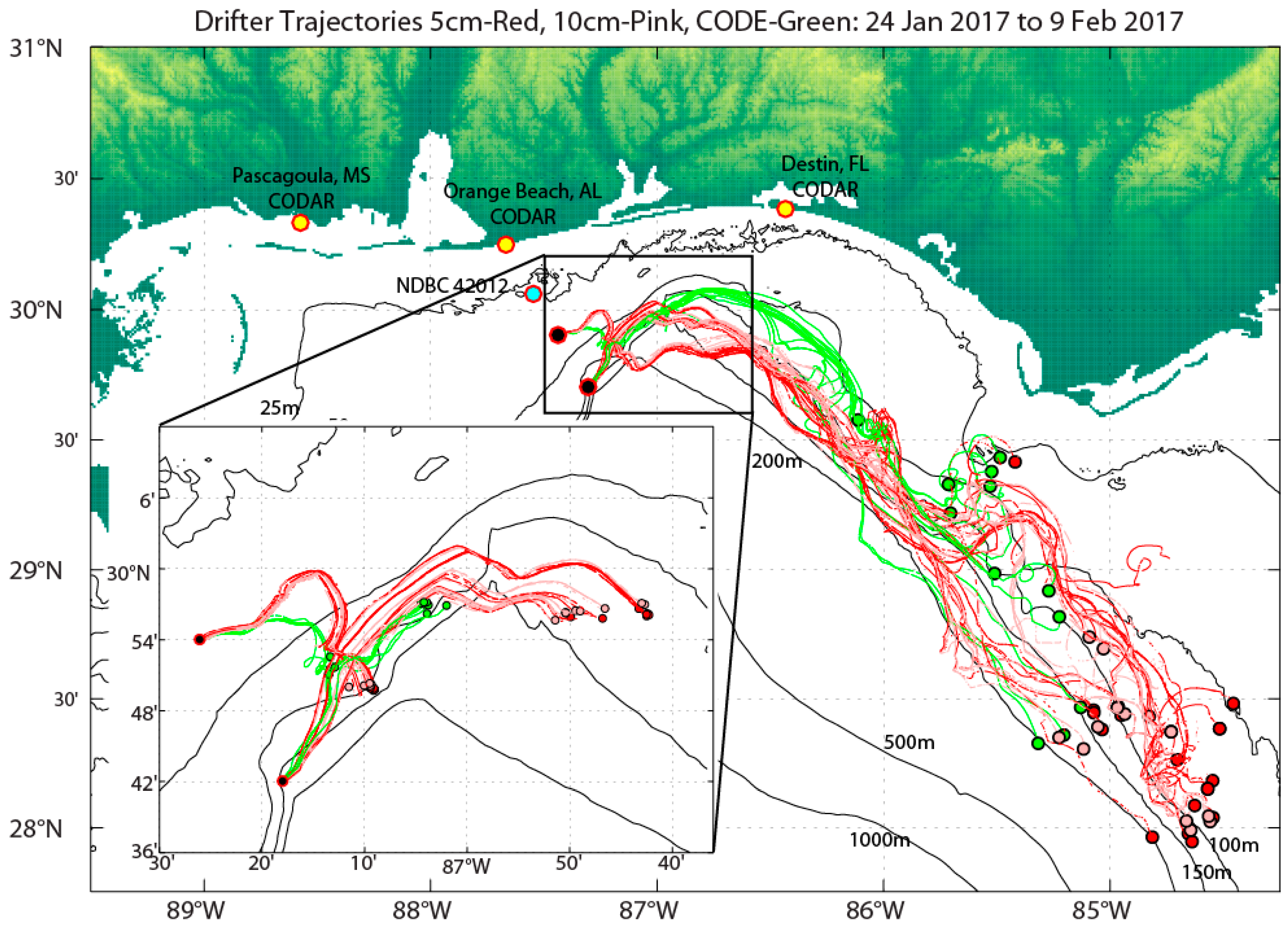
The primary goal of this work is to compare measurements of velocity near the sea surface using different approaches, including a new design for an ultra-thin satellite tracked drifter for measuring currents within a few centimeters of the ocean surface, and ideally to explain these differences. This drifter is designed to track the total Lagrangian surface velocity, which includes the Stokes drift velocity [9,10], and is intended for applications such as tracking contaminants on the sea surface and ground-truthing measurements of near-surface velocity from HF radar and new remote sensing technologies. This work presents analyses of measurements collected during a field experiment in the winter of 2017. In this experiment, thirty of these new drifters with hull height of 5 cm were deployed along with 28 similar drifters with hull heights of 10 cm and fourteen CODE- (Coastal Ocean Dynamics Experiment) or Davis-style drogued drifters [11] within the footprint of coastal HF radar over the shelf off of Orange Beach, AL (Figure 1). Collocated near-surface velocity observations from the drifters and the HF radar show substantial differences in the velocity measured by the different techniques. Analyses of the observations provide insight into the behavior of the near-surface drifters relative to other techniques for measuring near-surface currents. Understanding these differences is critical when using surface current measurements from different methods for applications such as surface material drift, air–sea flux calculations, and testing of new remote sensing technologies.
2. Materials and Methods
2.1. Drifters
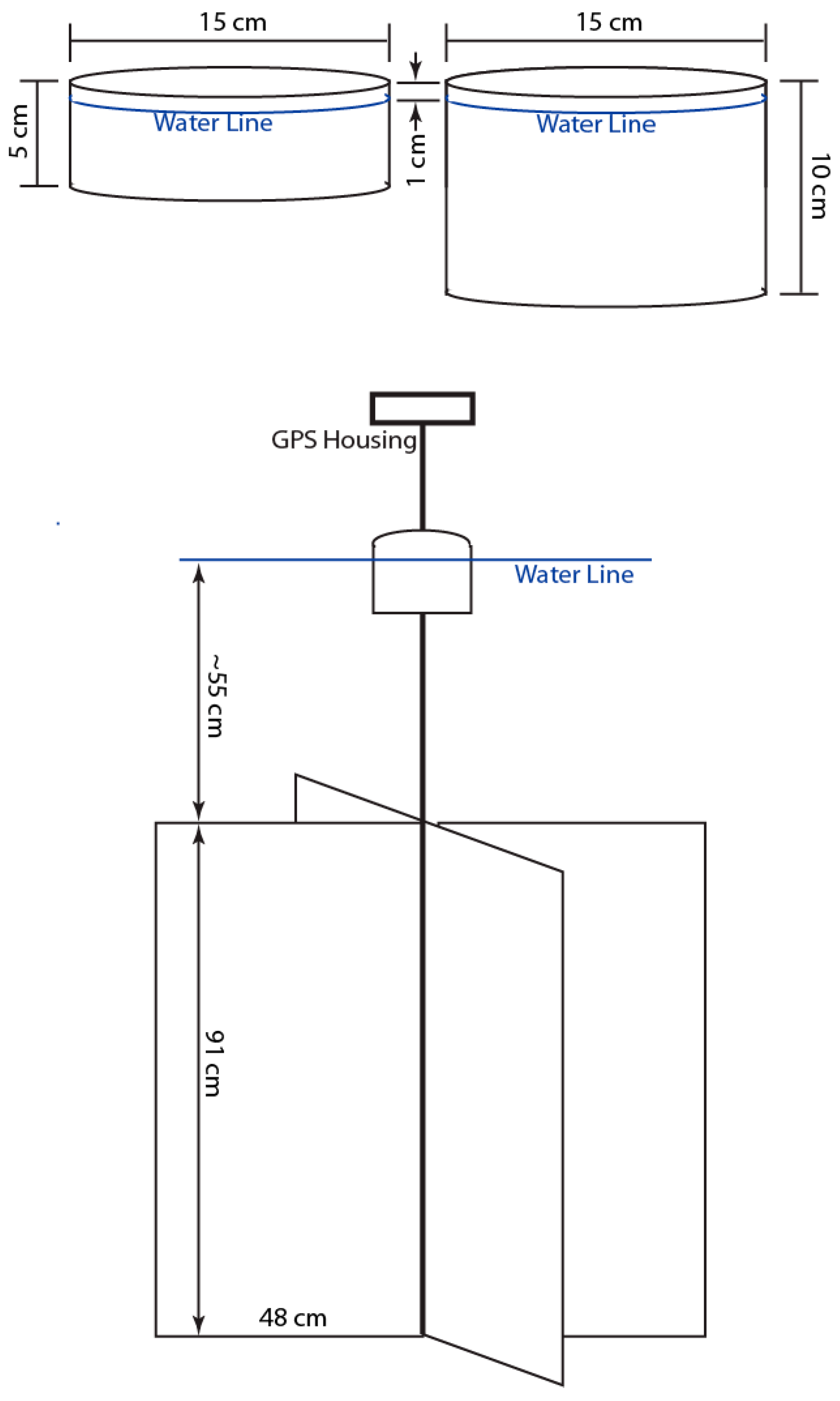
Thirty of the new ultra-thin drifters were constructed with a short cylindrical hull containing electronic components, batteries and ballast to be just buoyant with no more than 1 cm exposed above the sea surface (Figure 2). The hulls for the drifters used in this experiment were 15 cm in diameter and 5 cm high. The field experiment described here was conducted as an initial test of a new “flippable” drifter concept (patent pending), so the hulls were constructed from thin-walled PVC, serving as a proxy for the manufactured hulls of the final drifter design. A drifter with this small aspect ratio cannot be self-righting. Typically, surface drifters have been drogued or equipped with subsurface weight or floatation to keep them upright. However, these features hinder their ability to measure the current very near the ocean surface. When similarly thin drogued drifters have lost their drogues in the past, they could flip preventing them from transmitting [12]. Thus, the ultra-thin drifters developed for this project have as their innovation the ability to track and transmit regardless of their orientation.
This concept of a “flippable” ultra-thin drifter was tested during this field experiment by equipping each 5 cm drifter hull with two commercial GPS (Global Positioning System) satellite tracking/transmitting devices with custom software configuration, oriented toward each side of the drifter to be able to track and transmit regardless of orientation (the final drifter design uses only one satellite transmitting device to reduce communication component costs). Specifically, these drifters used SPOT Trace™ devices with custom programming installed by the manufacturer to allow them to continuously transmit positions via the GlobalStar® network at 5-min intervals.
An additional 28 cylindrical hull drifters were constructed in a similar fashion, but with 10 cm heights. These drifters were ballasted to be self-righting, requiring only one GPS tracker each. Finally, a set of fourteen CODE-style drifters (obtained from the Gulf of Maine Lobster Foundation: http://www.gomlf.org/drifters/) rounded out the set of drifters for this experiment. These drifters have canvas vanes extending from 0.5 to 1.5 m depth, and a GPS tracker affixed to a mast extending approximately 45 cm above the water surface.
The drifters were deployed on 24 January 2017 in two clusters: one on the shelf (30 m seafloor depth) 43 km south-southeast of Perdido Pass (Orange Beach, AL, USA), and the second over the shelf slope at the edge of DeSoto Canyon (170 m depth) 68 km offshore (Figure 1). Each deployment cluster consisted of seven CODE drifters, fifteen 5-cm drifters, and fourteen 10-cm drifters.
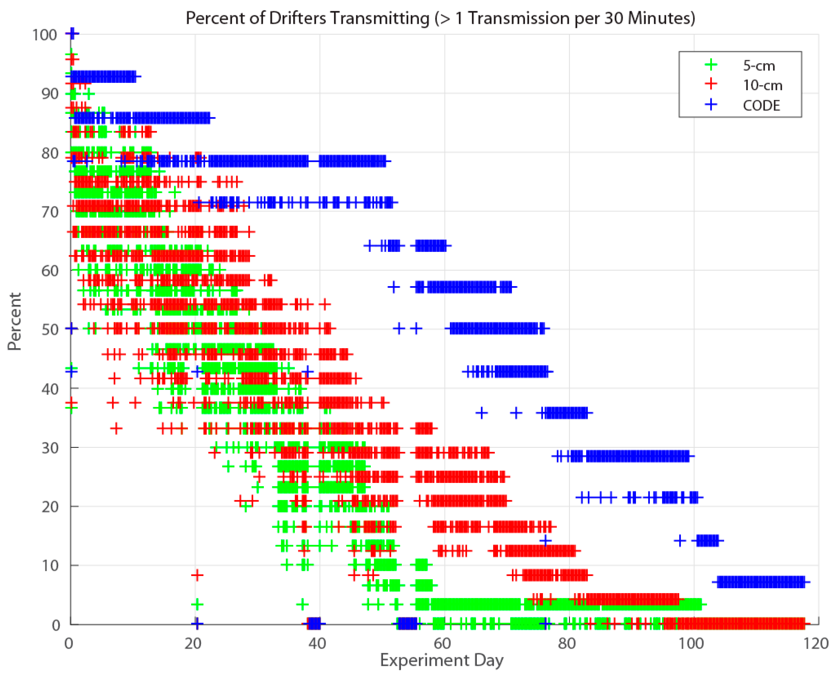
Drifters reported positions for 117 days (Figure 3) during the experiment with duration limited by battery life (compromised hulls may have also led to premature failure of some drifters). The 5-cm drifters failed at the fastest rate, likely due to the increased power consumption of the downward-oriented GPS trackers attempting to acquire satellite signals. (Note that issue does not affect a newer design of this drifter, as the instrument selectively uses only the upward-facing antennae). The CODE drifters generally transmitted the longest because they were equipped with higher capacity batteries. Drifter trajectory data are archived with the National Centers for Environmental Information (NCEI Accession Number 0175631).
2.2. HF Radar
The drifter deployment locations lie within the footprint of a coastal HF radar (4.54–4.75 MHz Long-Range CODAR—Coastal Ocean Dynamics Application Radar) operated by the University of Southern Mississippi. HF radar provides the near-surface velocity component in the radial direction (toward or away from the radar) inferred from movement of surface gravity waves with approximately one-half of the wavelength of the radar-transmitted signal [13,14]. Two-dimensional vector velocity is obtained by using measurements from two or more radar antennae installed at different locations. The USM CODAR installations are at Pascagoula, MS, Orange Beach, AL, and Destin, FL (Figure 1). This radar frequency band measures currents at approximately 2–3 m depth [15]. Hourly averaged 6-m binned vector currents over the drifter experiment region were obtained from the Coastal Observing Research and Development Center.
2.3. Analysis of Drifter Velocity
Following linear interpolation of drifter positions in time from their GPS timestamps to standard 5-min intervals, drifter velocities are computed from the differences in their positions per 5 min. Although the GPS trackers were programmed to transmit locations at 5-min intervals, failed transmissions lead to gaps. Interpolation of GPS positions to the standard 5-min intervals is performed for gaps of less than 30 min. Larger gaps in time are treated as missing data. Testing of the drifters fixed in place in water with small amplitude wind waves reveals a standard error in position measurements of approximately 4 m, which yields a standard error in velocity computed from 5-min positions of 1.9 cm/s. These velocity measurements are interpreted as the instantaneous velocity of the drifter halfway in time and space between the interpolated 5-min locations.
Drifter velocities are compared for pairs of co-located drifters of different types (5-cm and 10-cm drifters, and 5-cm and CODE drifters). Drifters are considered co-located if they are within 500 m of each other (different distance criteria for co-location have also been tested from 200 m to 1000 m resulting in only small differences in the results of these analyses). Overall, 95% of co-located pairs of 5-cm drifters and CODE drifter velocity measurements occur within the first 8 h of deployment, with no co-located measurements after 16 days. The 5-cm and 10-cm drifters more closely follow each other, with only 31% of co-located pairs of velocity measurements occurring within the first 8 h, 86% within the first 48 h, and no co-located measurements after 17 days.
The 10-cm or CODE drifter velocity rotated relative to the co-located 5-cm drifter velocity and scaled by the 5-cm drifter speed is computed as
where U and φ are the speed and course over ground (COG, clockwise from north, not to be confused with expressing angle in the typical mathematical sense of anti-clockwise from the positive x direction) of either 10-cm or CODE drifters, and U5 and φ5 are the speed and COG of the co-located 5-cm drifter. A scaled velocity of (urOrange Beachvr) = (0,1) indicates that the velocity of the drifter being compared is identical to the 5-cm drifter velocity. Non-zero values of ur indicate the COG of the drifter being compared is rotated relative to the 5-cm drifter COG. This quantity is only considered for co-located pairs of drifters where the speed of the 5-cm drifter exceeds 0.2 m/s to prevent dividing by small values.
For comparison with the HF radar velocity, drifter velocities are averaged in space and time to approximate the 6-km and hourly averaging of the radar velocity data. For each drifter type, all drifter velocity observations falling within a 6 km × 6 km region corresponding to the radar spatial bins and within 30 min of the timestamps of the HF radar velocity fields are averaged. Only averages of 15 or more drifter velocity measurements (reducing random errors to <0.5 cm/s) are compared to HF radar velocity measurements (given the 5-min drifter sampling, this ensures that averages include measurements from more than one drifter). The HF radar velocity relative to the bin-averaged velocity for each drifter type is computed for drifter speeds greater than 0.1 m/s. This lower speed threshold than used for the drifter-to-drifter comparisons is due to the relatively few numbers of co-located HF radar and binned drifter velocity measurements, but a consequence of using the lower speed threshold is greater scatter in the comparisons.
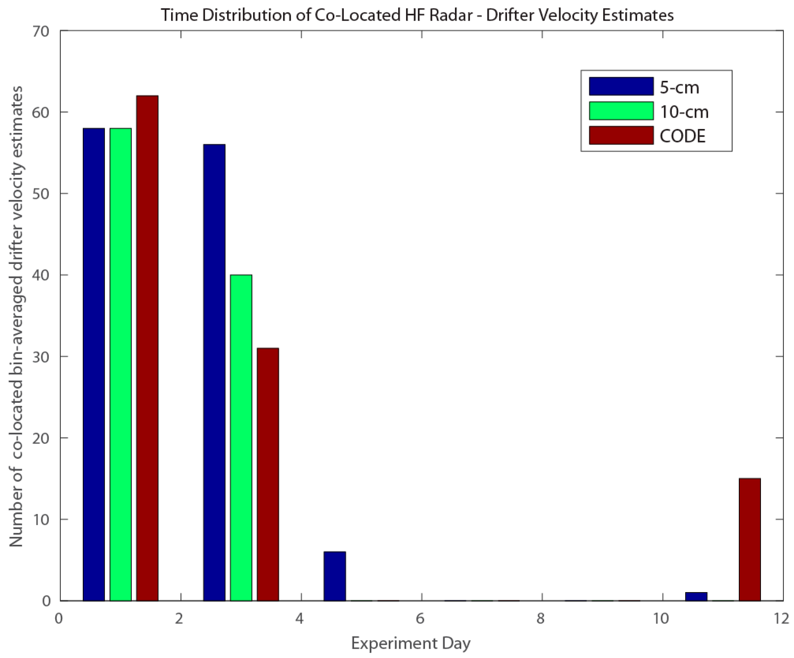
HF radar coverage varies spatially and in time with atmospheric and sea conditions. During the timeframe of this experiment, valid HF radar velocity data were obtained approximately 70% of the time near the drifter release location decreasing to only about 10% of the time along the drifter pathway at 86°W during this experiment (Figure 1). Thus, most of the co-located drifter and HF radar velocity estimates occurred during the first four days of the experiment (Figure 4).
2.4. Analysis of Stokes Drift
For this study, the Stokes drift was computed from the directional wave spectra measured at NDBC buoy 42012 (Figure 1) located near the drifter deployment locations, 22 km offshore of Orange Beach, AL, with seafloor depth of 26 m. The Stokes drift is computed from the wave spectra as [16]:
where σ is the angular frequency, θ is a wave direction, and F(σ, θ) is the wave spectrum. The discrete wave spectrum is determined from parameters archived by NDBC using the methods from [17]. The cutoff frequency σc is 3.05 rad/s. Consequences of computing the Stokes drift from the directional wave spectra versus the bulk wave characteristics more commonly obtained from buoy measurements are discussed in [18]. The Stokes velocity has a vertical profile of
where k is the wavenumber. The Stokes velocity acting on the drifters is computed as Us(z) averaged over the drifter profile or drogue depth (4 cm for the 5-cm drifters, or 55–146 cm for CODE drifters). In the analysis presented here, the vertical decay profile is computed for each directional and frequency bin of the wave spectrum.
3. Results
3.1. Drifter Trajectories and Velocity
The field experiment took place during winter when the northern Gulf of Mexico experiences strongly variable meteorological and oceanographic conditions. Atmospheric cold fronts and extratropical cyclones dominate the synoptic variability of winds over this region during this time, with winds alternating from southerly (northward) ahead of a cold front and rapidly turning clockwise to northerly (southward) following passage of the front (Figure 5). Asymmetry in the strength of the northward and southward winds (southward being stronger) promotes a residual jet flowing southeastward along the shelf of the northeastern Gulf [19]. This circulation pattern is revealed in the general direction of trajectories of the drifters (Figure 1).
The drifter trajectories (Figure 1) show that, in general, the 5-cm and 10-cm drifters tracked closely together, deviating from the CODE drifter trajectories (particularly evident near the deployment locations). Additionally, the thin surface drifters generally travelled further than the CODE drifters over the same period, indicating that they had a greater average speed.
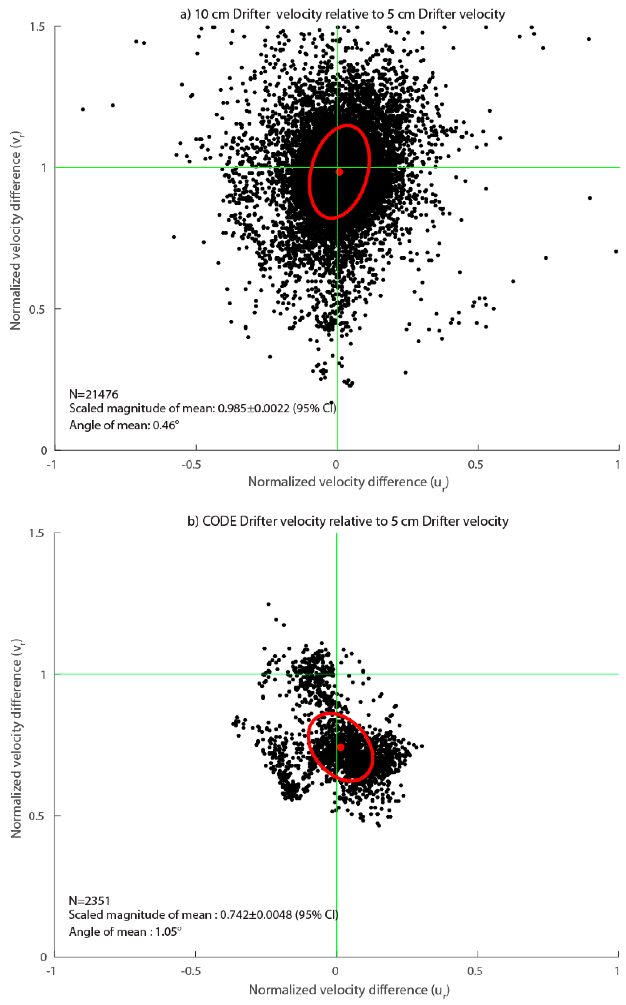
A scatter plot comparing the velocities of co-located pairs of 5-cm and 10-cm drifters (Figure 6, top) shows that they have very similar behavior. The 10-cm drifter velocities have, on average, a magnitude that is 98.5% of to the co-located 5-cm drifter velocities, and their directions nearly identical (on average, the 10-cm drifter velocity is rotated 0.46° clockwise from the 5-cm drifter velocity). In contrast, the CODE-style drifter velocity magnitude is an average of only 74.2% that of the 5-cm drifter velocity (Figure 6, bottom), rotated 1.05° clockwise.
To interpret Figure 6 and similar plots, the angle between a vector drawn from the origin to the red dot and a vector from the origin to (0,1) gives the mean deviation in direction of the drifter velocity being compared relative to the 5-cm drifter velocity. Similarly, the magnitude of this vector to the red dot indicates the mean magnitude of the compared drifter velocity relative to the 5-cm drifter velocity. Spread in the scatter plots are due to several factors, but particularly differences in currents between drifter location (distances between “co-located” drifters can be up to 500 m apart for this analysis) and measurement errors. Scatter can be reduced by considering a closer distance threshold for drifter co-location or averaging velocity over a longer time interval than the 5-min drifter measurements, but this reduces the number of co-located drifter pairs increasing the uncertainty, particularly for the comparison between the CODE and 5-cm drifters.
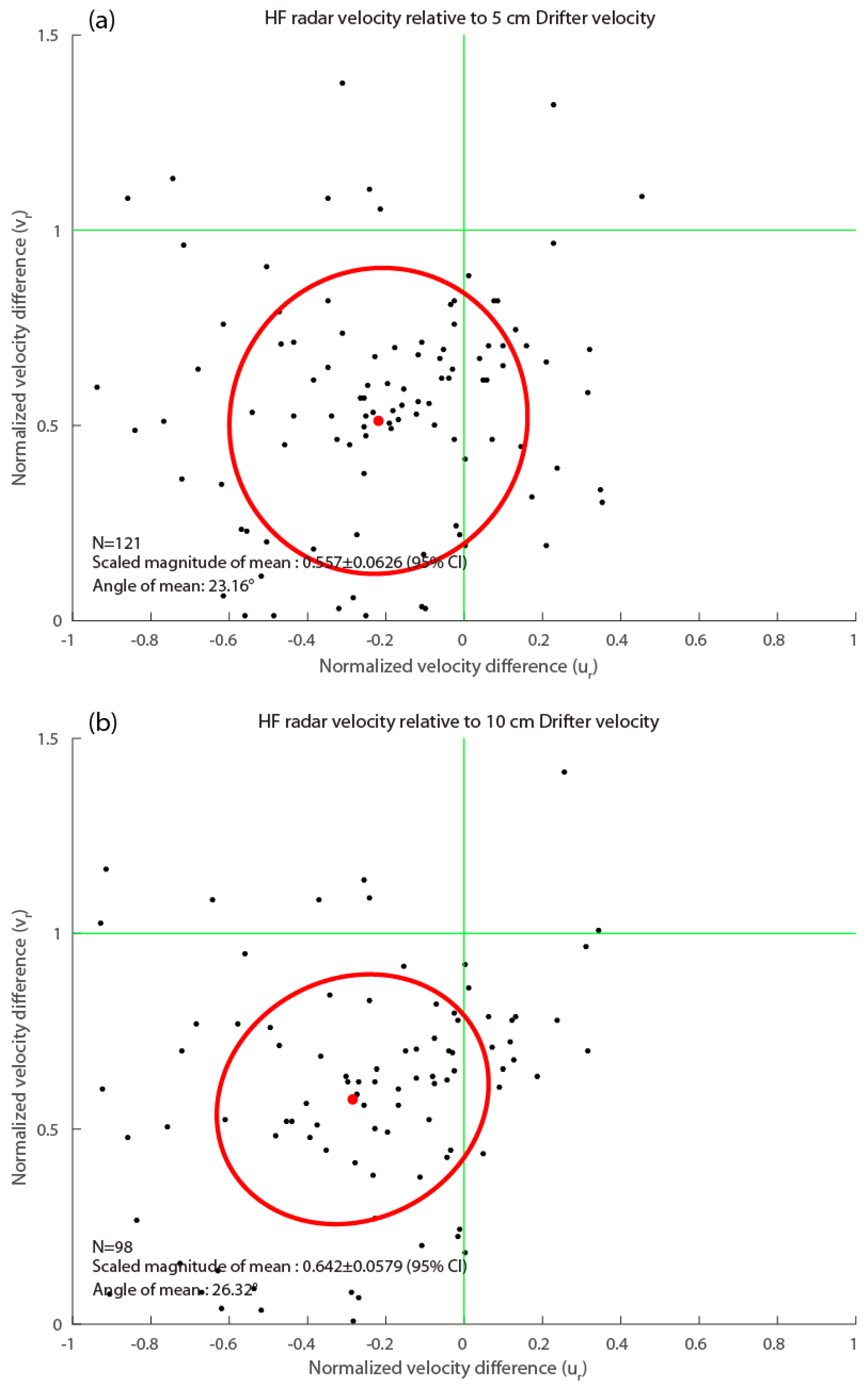
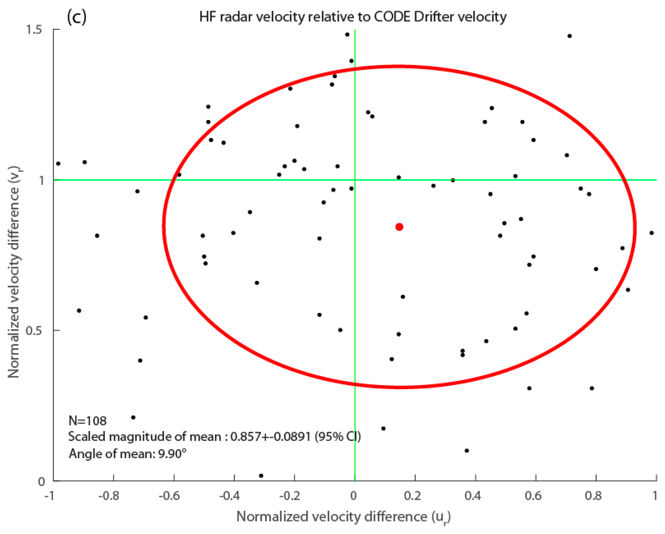
Similar comparisons are made between the surface velocity measurements from the HF radar and each of the drifter types (Figure 7). Because the velocity measurements are averaged hourly over 6-km bins, there are substantially fewer pairs of velocity measurements for analysis. Additionally, the drifters inadequately sample the currents over a 6-km-by-6-km region in 1 h, so their representativeness of the bin-averaged currents is likely poor. This increases the scatter of the co-located scaled velocity measurements comparing the HF radar velocity to the drifters. Nevertheless, the scatter plots reveal significant and systematic differences between the remotely sensed surface currents and the currents measured by each of the drifter types.
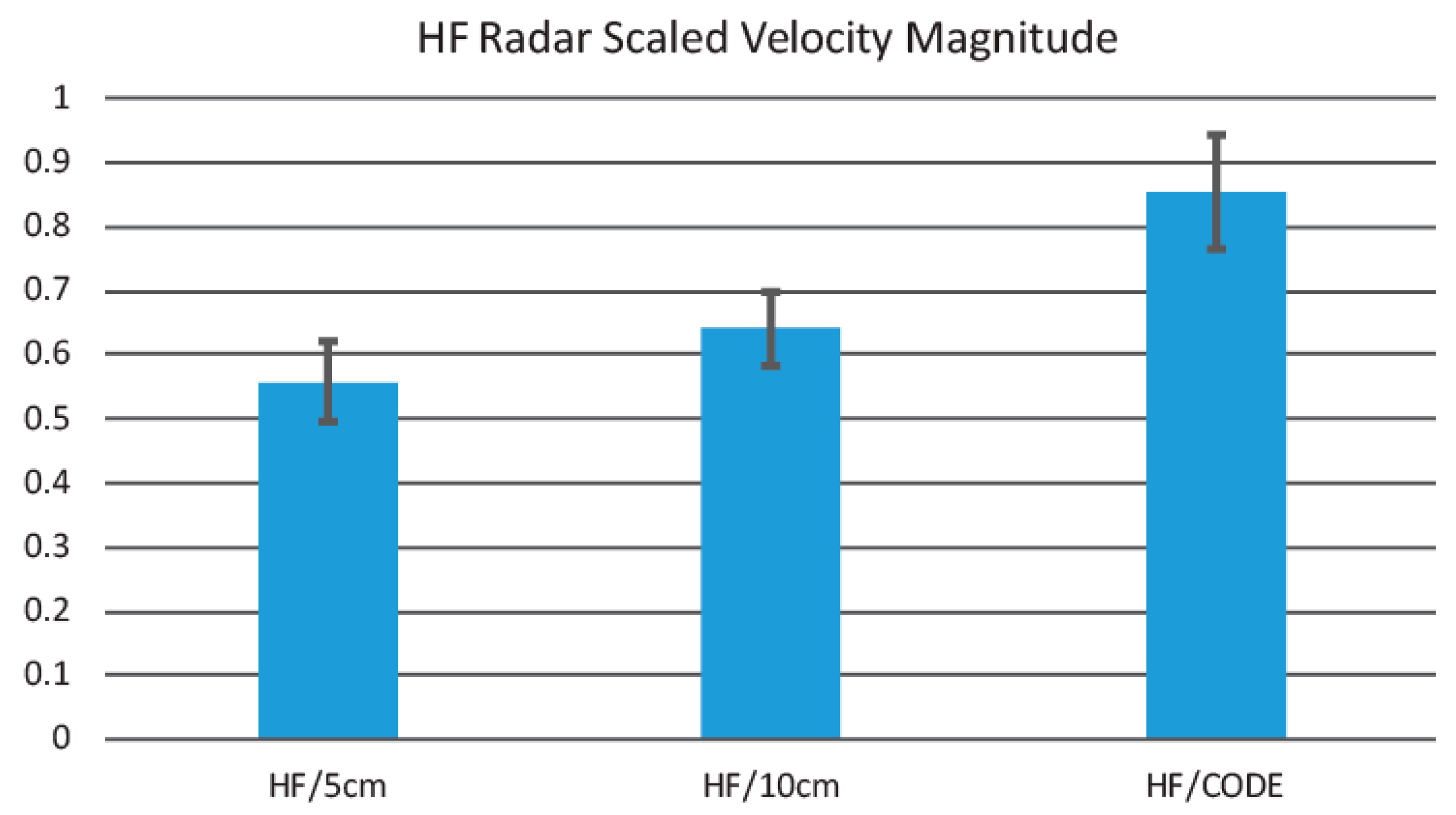
On average, the HF radar velocity magnitude is only 55.7% (±6.26, 95% CI) of bin-averaged 5-cm drifter velocity measurements (Figure 7a and Figure 8), and is directed 23.16° anticlockwise. Similarly, the HF radar velocity magnitude is on average 64.2% (±5.79) of the 10-cm drifter bin-averaged velocity magnitude, directed 26.32° anticlockwise. The HF radar velocity measurements are much closer to the CODE drifter velocities, with HF radar velocity magnitude 85.7% (±8.91) that of the CODE drifters, directed 9.9° clockwise. Due to the large scatter in the co-located velocity measurements (illustrated by the large standard deviation ellipses on the scatter plots in Figure 7) and poor representativeness of bin-averaged currents from drifter measurements, there is substantial uncertainty in these statistics (as shown by error bars in Figure 8 and listed on each plot of Figure 7). However, the analysis shows systematically growing significant differences between the HF radar velocity and the Lagrangian velocity measured by drifters at diminishing depths below the surface.
3.2. Stokes Drift
The 5-cm drifter deployed during this experiment has characteristics that should allow it to measure the total surface velocity including the Stokes drift. The Stokes drift velocity decays exponentially from the surface with depth dependent on the wave number, but, for typical wavelengths during this experiment, the average of the Stokes drift velocity over the submerged depth of the drifter (4 cm) is over 99% that at the surface. The magnitude of the Stokes drift is also related to the wave frequency, with higher frequency (shorter waves) resulting in greater drift velocity. As such, the small diameter of the 5-cm drifter allows it to follow more closely the trajectory of a hypothetical Lagrangian particle in a wave field with very short waves than would a drifter with wider dimension.
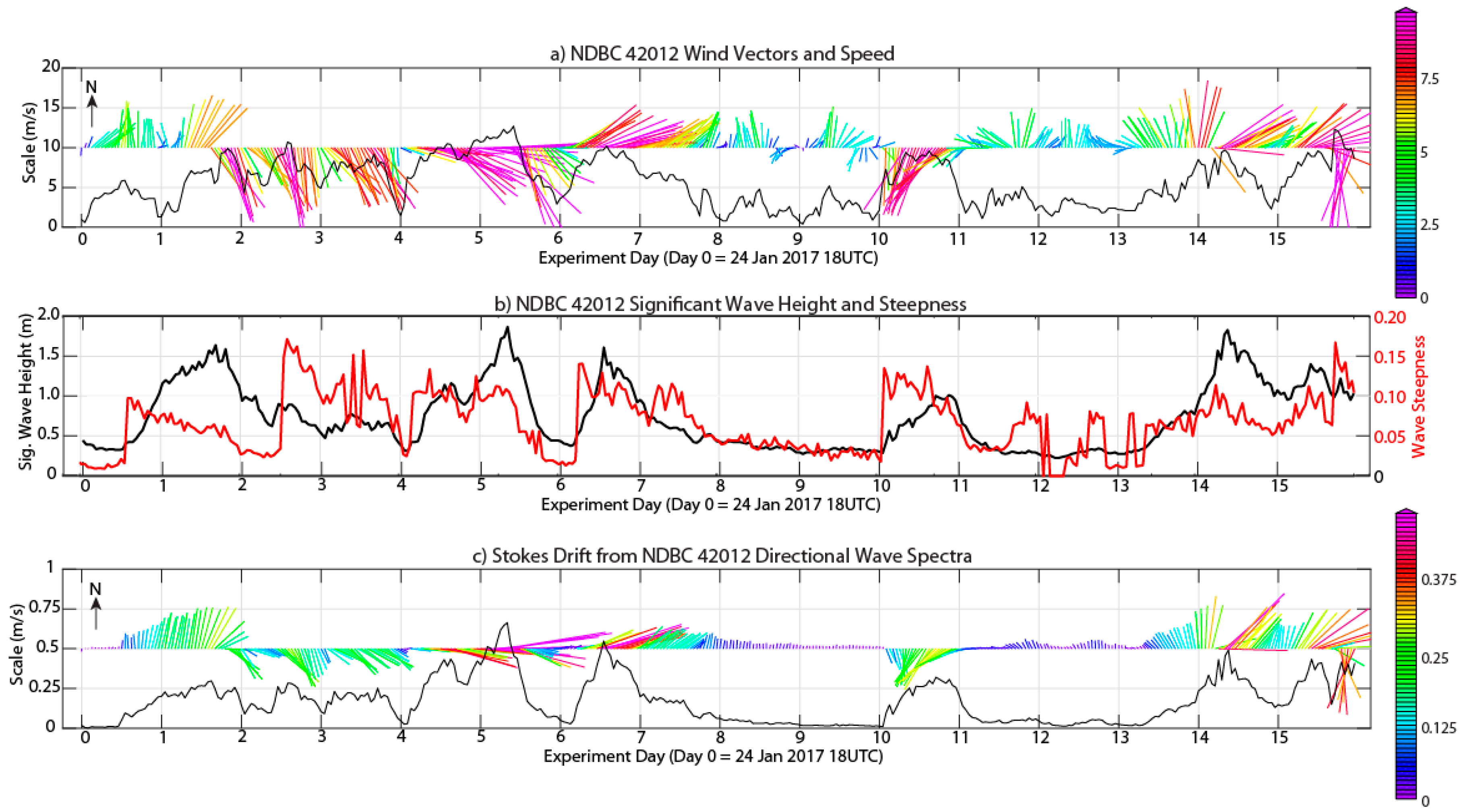
The wave field in the northern Gulf of Mexico is dominated by wind waves, with swell generally only occurring when storms are active elsewhere within this semi-enclosed basin. The surface Stokes drift roughly follows the direction of the local winds at NDBC 42012 (Figure 5). Notable is the lack of Stokes drift during the first 12 h following deployment. Unfortunately, this was the period during which most co-located drifter velocity observations are available. To assess the impact of Stokes drift on the drifter velocity measurements, the distance threshold for considering drifters co-located is increased to 4000 m (from 500 m used for the above analyses), and only co-located drifter velocity measurements occurring later than 12 h after deployment are considered (otherwise, the results are biased due to the vast majority of co-located drifter observations occurring during this time of nearly zero Stokes drift).
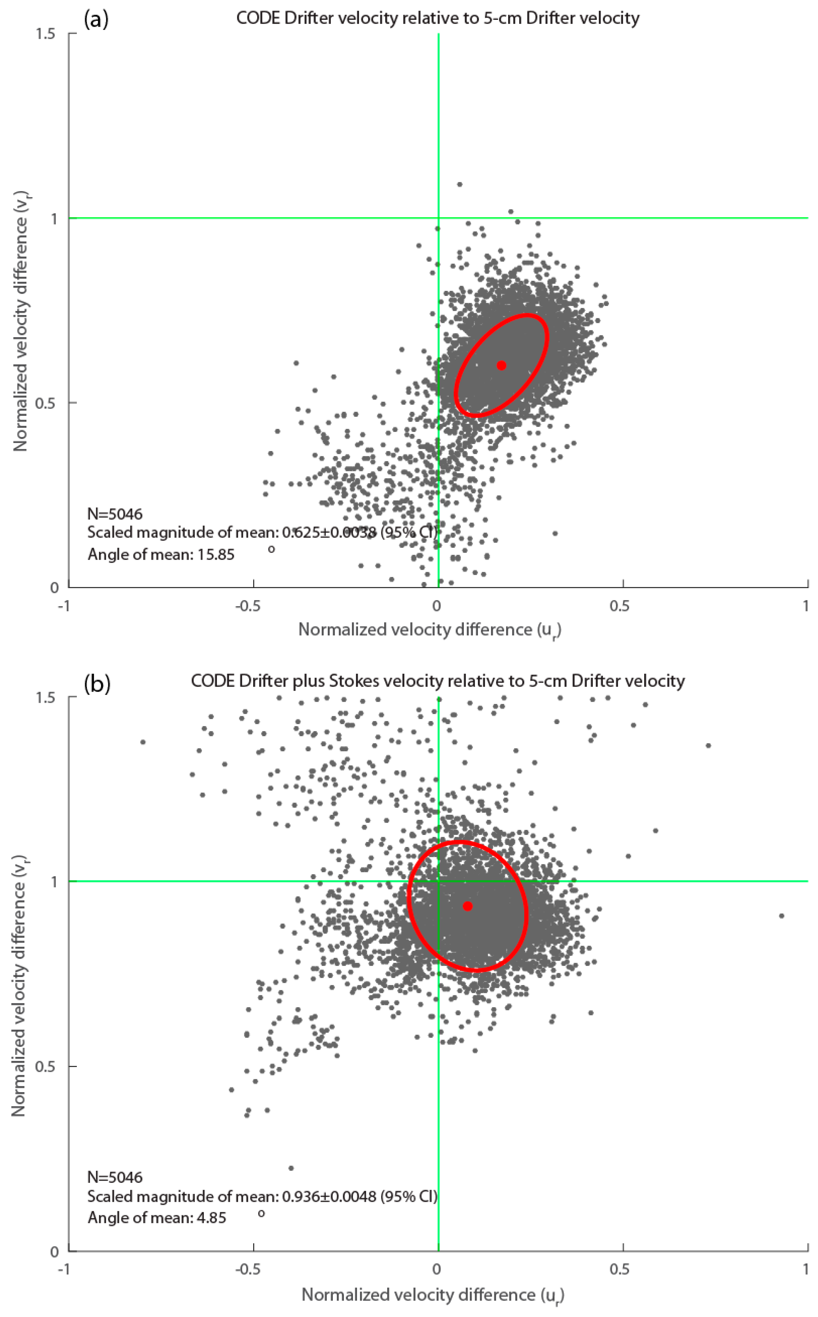
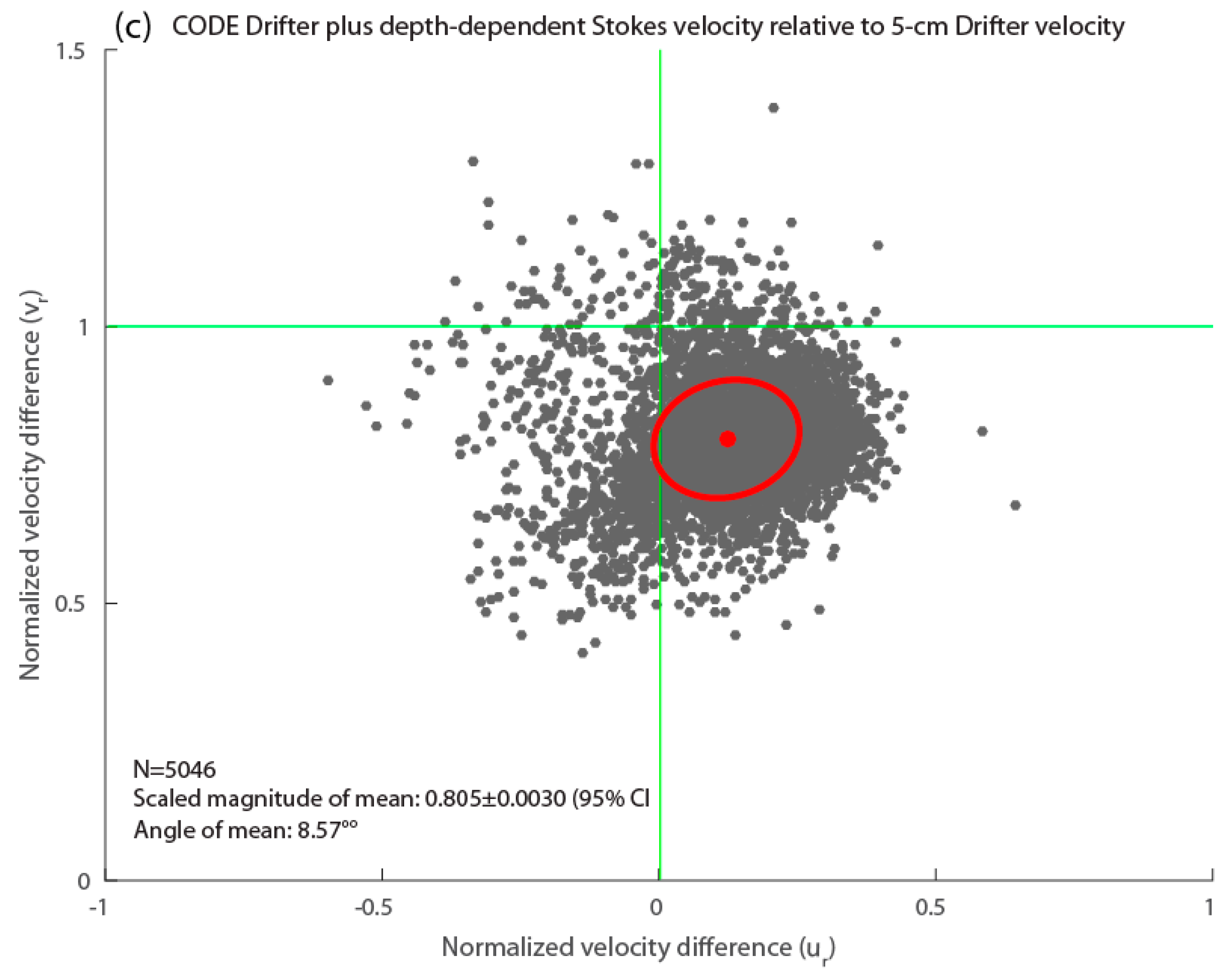
Considering this new set of co-located velocity measurements, the magnitude of the mean CODE-drifter velocity relative to the 5-cm drifter velocity is 0.625 (Figure 9a), compared to 0.742 when including measurements from the first 12 h (Figure 6). The mean CODE-drifter velocity is rotated 15.85° clockwise relative to the 5-cm drifter velocity. Adding the Stokes drift velocity of the upper 4 cm to the CODE drifter velocity results in a much closer match to the 5-cm drifter velocity (Figure 9b). The magnitude of the mean CODE-drifter velocity adjusted for Stokes drift is now 93.6% of the 5-cm drifter velocity, and the rotation angle has decreased to 4.85°. This adjustment, however, does not consider the possibility of Stokes drift also acting on the CODE drifters. An analysis of the impact of Stokes drift on a drifter with similar configuration is presented by Davis [20]. When the CODE drifter velocity is adjusted for the theoretical difference of the Stokes drift acting on the 4-cm drifters versus on the CODE drifters, the mean adjusted velocity magnitude is 80.5% that of the 5-cm drifters, and the mean rotation is 8.57° clockwise (Figure 9c). That is, under the assumption that the CODE drifters effectively measure the Stokes drift velocity acting over their drogue depths, this analysis suggests that there are additional sources of shear in the near-surface velocity, for example Langmuir and Ekman layer shear [21]. This discrepancy may also be due to the CODE drifter not precisely following the Stokes drift due to characteristics of its design, including the larger lateral dimensions of the drogue compared to the very short wind waves that contribute strongly to the Stokes drift.
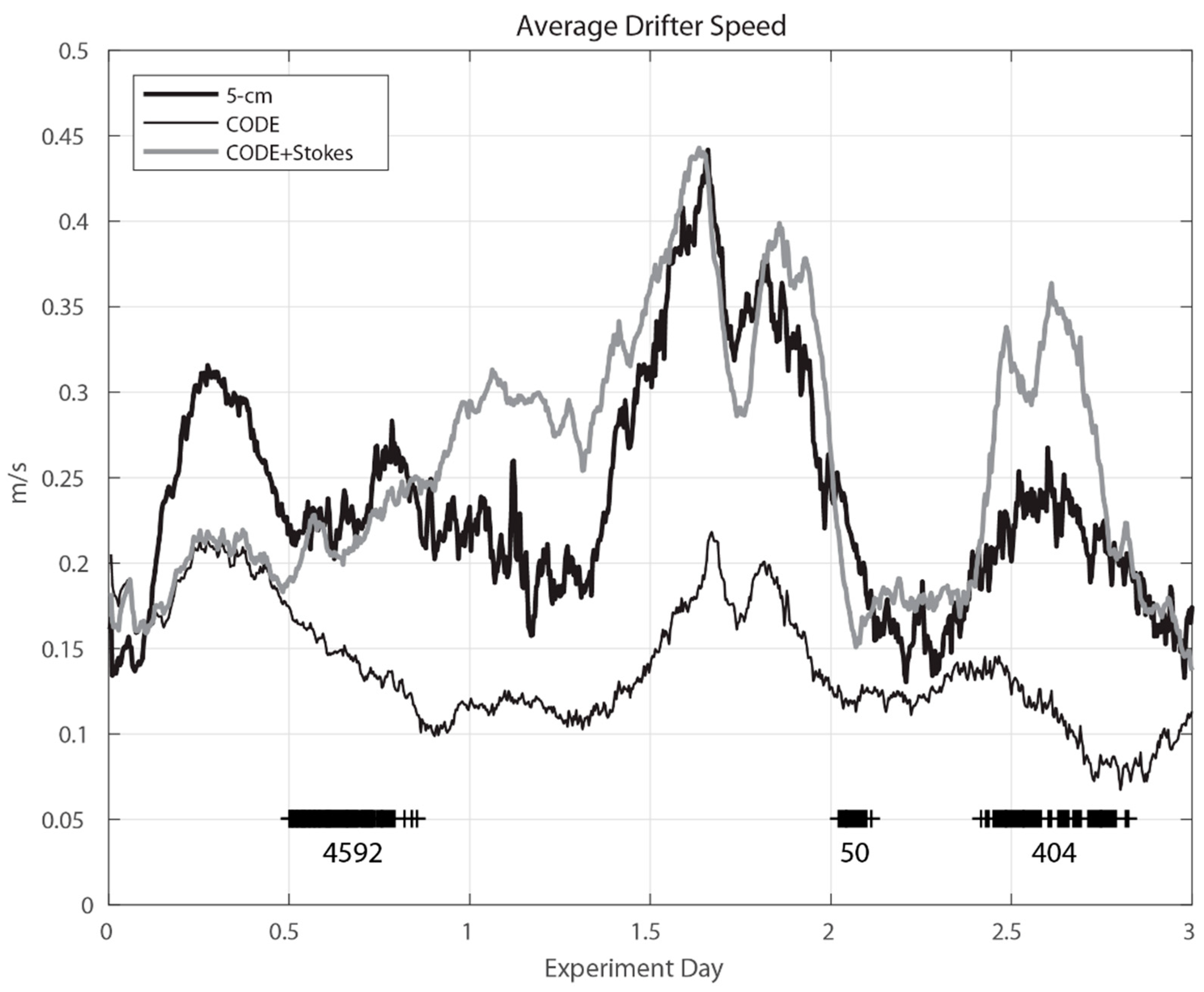
Although adding the surface Stokes drift velocity to the CODE drifter velocity results in a much closer match to the 5-cm drifter velocity on average, there are several outliers (Figure 9b) that indicate that at times this adjustment may not be appropriate. All co-located drifter velocity observations presented in Figure 9 occur between 12 h and three days after deployment, but with clustering in three periods of several hours each (black plus symbols in Figure 10). Overall, 91% of these co-located observations occurs one-half to one day into the experiment, 8% of them 2.4–2.8 days into the experiment, and the remaining 1% just after two days into the experiment. During this three-day period, the forward speed averaged over all of the 5-cm drifters for each time was consistently higher than the average speed of all of the CODE-style drifters (Figure 10). The average magnitude of the CODE drifter velocity adjusted by addition of the surface Stokes drift velocity much more closely matches the average speed of the 5-cm drifters during much of the period, but with some important exceptions. One of these exceptional periods is around Day 2.5, when the Stokes-adjusted CODE drifter velocity magnitude is 5–10 cm/s higher than the 5-cm drifter speed. This period corresponds to times of co-located velocity observations that appear as outliers in Figure 9b.
During the first 12 h (during which the Stokes drift was nearly zero), the average speed of all the 5-cm drifters was up to 10 cm/s faster than the CODE drifters. It is not clear whether this is due to strong near-surface shear unrelated to Stokes drift, or to the drifters possibly being in regions of differing currents. One of the deployment locations was near the shelf edge where there could be strong horizontal gradients in currents, although analysis of co-located drifter pairs suggests that the 5-cm drifters were indeed traveling faster than their co-located CODE-style counterparts. This result differs from the suggestion by Ardhuin et al. [22] that shear of the Eulerian wind-driven current in the upper meter is small compared to the Stokes velocity shear (which during the period at the beginning of the experiment was negligible).
Around 2.5 days into the experiment, the Stokes-adjusted CODE-velocity magnitudes are substantially higher than the average 5-cm drifter speed. The wind had turned out of the north several hours earlier due to a cold front passage, but, at this time, the wind speed increased even more to over 10 m/s and the dominant wave period also dropped abruptly from 8 s to 3 s. Given the proximity of the coast to the north, these waves are fetch-limited and very steep, leading to wave breaking. Indeed, the wave steepness, computed as
where Hs is the significant wave height and k is the wavenumber associated with the dominant wave period, rapidly increases from 0.03 to >0.15 (Figure 5). As shown by Banner et al. [23], wave breaking begins to occur for ε > 0.05. Although wave breaking does not affect the vertically integrated Lagrangian momentum due to wave motions, it does result in a change in the Stokes drift profile [24]. Essentially, wave breaking mixes momentum from the surface to the ocean’s interior breaking down the classic depth profile for Stokes drift. This explains why, during wave breaking conditions, the forward speed of the CODE drifters more closely matches the 5-cm drifters, and adding a Stokes drift velocity to the CODE drifter velocity results in a much higher speed than the 5-cm drifters.
4. Discussion and Conclusions
Measurements of currents at depths of one to several meters are useful for a number of practical and scientific applications. These currents more strongly affect objects on the surface with greater depth extents (e.g., ships), are more comparable to the upper layer currents simulated in ocean models (and thus more suitable for data assimilation), and more closely related to the underlying geostrophic currents that can be inferred from other data sources (e.g., satellite altimetry). However, there are important emerging applications requiring knowledge of currents at the very surface of the ocean. These include improved methods of determining air–sea momentum and heat fluxes and determining transport of material at the ocean surface (e.g., oil slicks and buoyant organisms). New remote sensing technologies will provide measurements of this variable [6,7], but in situ measurements have not previously been widely available for calibration/validation purposes. Further, a better understanding of the vertical shear near the ocean surface and impacts on more widely available Lagrangian and HF radar measurements is needed so that these measurements can better be used for application requiring knowledge of the total surface currents. The ultra-thin small satellite-tracked drifter used for this study may provide an inexpensive method of obtaining measurements of the total Lagrangian surface current for large-scale applications.
The new ultra-thin drifter design has been tested in open-ocean field experiments such as the one reported here. However, for future applications, such as validating Doppler scatterometry-measured surface currents, it would be useful to first test the drifter in a carefully designed laboratory study to verify that the drifter accurately follows the total surface current under different wind and wave conditions. Such a study might be accomplished using a particle image velocimetry (PIV) method in a wave and current tank. However, in the absence of such laboratory testing, it is worth noting that this drifter design very closely matches the traits of an “ideal” drifter for measuring surface currents as described by [20]. That is, the drifter: (1) has minimum structure above the surface; (2) is a flat disk floating on the surface which gives it a high natural heave frequency with significant damping; (3) is small compared to the scale of horizontal velocity shear associated with small gravity waves; and (4) follows the tilt of the wave surface. Adherence to these design concepts provides confidence that the ultra-thin drifter accurately follows the total surface current.
A striking result of this study is the disparate measurements of surface currents obtained from the new drifters and two other commonly used technologies—the shallow drogued drifter and coastal HF radar. The drogued drifter and the HF radar surface velocity measurements were quite similar, with the HF radar measuring currents with magnitude approximately 14% (±9%) weaker than the drogued CODE-style drifter. However, this small difference may be due to the HF radar effectively measuring currents at a depth approximately one meter deeper than the drogued drifter. HF radars with different frequencies than that used here have velocity measurements with better or worse agreement to these drifter velocities.
The 5- and 10-cm thin drifters, while having velocity measurement characteristics very similar to each other, measured surface currents that were on average substantially stronger than those measured by the HF radar or drogued drifters. Notably, the velocity magnitudes measured by the drogued drifters and the thin drifters are very similar during times of wave breaking, as wave breaking results in a reduction of near-surface shear of the Stokes velocity. However, when wave breaking is not occurring, the surface Stokes drift appears to account for much of the discrepancy between the drogued drifter velocity and the thin surface drifters. This assumes that the impact of Stokes drift on the drogued drifters is negligible, an assumption supported by the analysis of Kenyon [10], but differing from some previous studies [25,26]. A possible explanation is that the thin drifters have very small diameters, allowing them to closely follow orbital trajectories of very short surface gravity waves. In contrast, the CODE-style drifters have much larger dimensions such that they do not exactly follow the oscillating motions associated with the very short waves that are common in the northern Gulf, particularly during periods of offshore (northerly) winds. A more careful study of the performance of similar drifters in similar wave conditions is warranted.
An interesting observation is the large discrepancy in velocity measured by the drogued drifters and the thin drifters during the early hours of the experiment when the Stokes drift was negligible (Figure 1 and Figure 10). What gave rise to this apparent strong near-surface shear remains unknown. It is worth noting that during preliminary field testing of the drifters over a shallow (4-m deep) microtidal grass flat with calm seas and very light (<2 m/s) winds, the 5-cm and 10-cm drifters traveled at approximately 120° relative to one another, separating at a rate of nearly 20 cm/s for about 1 h. Indeed, this is a very different environment from the mid- and outer-shelf deployment region for this study, but this is evidence that very strong shear can occur between the depths measured by the CODE-style drifters and the thin surface drifters. Given the common use of these drogued drifters and similarly performing coastal HF radar for measuring surface drift, such traits should be carefully considered.
A recent study by Lund et al. [27] compared velocity measurements from shallow (0.4 m) drogued drifters used by Novelli et al. [12] with shipboard x-band radar (measuring an effective depth of 1–5 m) and the results yielded an rms difference of current speed of only 4 cm s−1. This is much less than the difference between the ultra-thin drifter speeds and the CODE-style drifter and HF radar speeds analyzed here. This supports that the strongest shear occurs much closer to the surface than 0.4 m, as would be expected from the theoretical exponential decay profile of Stokes drift velocity (Equation (2)).
Author Contributions
Conceptualization, S.L.M. and N.W.; Methodology, S.L.M., N.W., D.S.D. and M.A.B.; Software, S.L.M. and D.S.D.; Formal Analysis, S.L.M. and D.S.D.; Investigation, S.L.M., N.W., and D.S.D.; Data Curation, S.L.M. and N.W.; Writing—Original Draft Preparation, S.L.M.; Writing—Review and Editing, S.L.M., N.W., D.S.D., and M.A.B. Visualization, S.L.M.; Supervision, S.L.M. and N.W.; Project Administration, S.L.M.; and Funding Acquisition, S.L.M., N.W., D.S.D., and M.A.B.
Funding
This research was funded by NOAA grant award NA15OAR4320064 to the University of Miami Cooperative Institute for Marine and Atmospheric Studies, sub-awarded to Florida State University as project “Development of New Drifter Technology for Observing Currents at the Ocean Surface”.
Acknowledgments
The authors would like to acknowledge the assistance of J. Caleb Hudson and John Easton in developing and assembling the drifters, and to Captain Tristan Ellis and Mate Preston Gray of the vessel Southerner of Reel Surprise Charters in Orange Beach, AL, for expertly assisting with the drifter deployment.
Conflicts of Interest
The authors declare no conflict of interest. The funders had no role in the design of the study; in the collection, analyses, or interpretation of data; in the writing of the manuscript, and in the decision to publish the results.
References
- Chapman, R.D.; Shay, L.K.; Graber, H.C.; Edson, J.B.; Karachintsev, A.; Trump, C.L.; Ross, D.B. On the accuracy of HF radar surface current measurements: Intercomparisons with ship-based sensors. J. Geophys. Res. 1997, 102, 737–748. [Google Scholar] [CrossRef]
- Teague, C.C.; Vesecky, J.F.; Hallock, Z.R. A comparison of multifrequency HF radar and ADCP measurements of near-surface currents during COPE-3. IEEE J. Ocean. Eng. 2001, 26, 399–405. [Google Scholar] [CrossRef]
- Churchill, J.H.; Csanady, G.T. Near-surface measurements of quasi-Lagrangian velocities in open water. J. Phys. Oceanogr. 1983, 13, 1669–1680. [Google Scholar] [CrossRef]
- Bye, J.A. Wind-driven circulation in unstratified lakes. Limnol. Oceanogr. 1965, 10, 451–458. [Google Scholar] [CrossRef] [Green Version]
- Bye, J.A. The coupling of wave drift and wind velocity profiles. J. Mar. Res. 1988, 46, 457–472. [Google Scholar] [CrossRef]
- Rodríguez, E.; Wineteer, A.; Perkovic-Martin, D.; Gál, T.; Stiles, B.W.; Niamsuwan, N.; Monje, R.R. Estimating Ocean Vector Winds and Currents Using a Ka-Band Pencil-Beam Doppler Scatterometer. Remote Sens. 2018, 10, 576. [Google Scholar] [CrossRef]
- Ardhuin, F.; Aksenov, Y.; Benetazzo, A.; Bertino, L.; Brandt, P.; Caubet, E.; Chapron, B.; Collard, F.; Cravatte, S.; Delouis, J.M.; et al. Measuring currents, ice drift, and waves from space: The Sea surface Kinematics Multiscale monitoring (SKIM) concept. Ocean Sci. 2018, 14, 337–354. [Google Scholar] [CrossRef]
- Samuels, W.B.; Huang, N.E.; Amsiuiz, D.E. An oil spill trajectory analysis model with a variable wind deflection angle. Ocean Eng. 1982, 4, 347–360. [Google Scholar] [CrossRef]
- Stokes, G.G. On the theory of oscillatory waves. Trans. Camb. Phil. Soc. 1847, 8, 441–455. [Google Scholar]
- Kenyon, K.E. Stokes drift for random gravity waves. J. Geophys. Res. 1969, 74, 6991–6994. [Google Scholar] [CrossRef]
- Davis, R.E. Drifter observations of coastal surface currents during CODE: The statistical and dynamical views. J. Geophys. Res. 1985, 90, 4756–4772. [Google Scholar] [CrossRef]
- Novelli, G.; Guigand, C.M.; Cousin, C. A biodegradable surface drifter for ocean sampling on a massive scale. J. Atmos. Ocean. Technol. 2017, 34, 2509–2532. [Google Scholar] [CrossRef]
- Stewart, R.H.; Joy, J.W. HF radio measurements of surface currents. Deep Sea Res. Ocean. Abstr. 1974, 21, 1039–1049. [Google Scholar] [CrossRef]
- Ohlmann, C.; White, P.; Washburn, L.; Terrill, E.; Emery, B.; Otero, M. Interpretation of coastal HF radar-derived surface currents with high-resolution drifter data. J. Atmos. Ocean. Technol. 2007, 24, 666–680. [Google Scholar] [CrossRef]
- Laws, K. Measurements of Near Surface Ocean Currents Using HF Radar. Ph.D. Thesis, The University of California at Santa Cruz, Santa Cruz, CA, USA, 2001. [Google Scholar]
- Tamura, H.; Miyazawa, Y.; Oey, L.-Y. The Stokes drift and wave induced mass flux in the North Pacific. J. Geophys. Res. 2012, 117, C08021. [Google Scholar] [CrossRef]
- Earle, M.D.; Steele, K.E.; Wang, D.W.C. Use of advanced directional wave spectra analysis methods. Ocean Eng. 1999, 26, 1421–1434. [Google Scholar] [CrossRef]
- Kumar, N.; Cahl, D.L.; Crosby, S.C.; Voulgaris, G. Bulk versus spectral wave parameters: Implications on Stokes drift estimates, regional wave modeling, and HF radars applications. J. Phys. Oceanogr. 2017, 47, 1413–1431. [Google Scholar] [CrossRef]
- Todd, A.C.; Morey, S.L.; Chassignet, E.P. Circulation and cross-shelf transport in the Florida Big Bend. J. Mar. Res. 2014, 72, 445–475. [Google Scholar] [CrossRef]
- Davis, R.E. An inexpeinsive drifter for surface currents. In Proceedings of the 1982 IEEE Second Working Group Conference on Current Measurement, Hilton Head, SC, USA, 19–21 January 1982; IEEE: Piscataway, NJ, USA, 1982; Volume 2. [Google Scholar]
- McWilliams, J.C.; Huckle, E.; Liang, J.-H.; Sullivan, P.P. The wavy Ekman layer: Langmuir circulations, breaking waves, and Reynolds stress. J. Phys. Oceanogr. 2012, 42, 1793–1816. [Google Scholar] [CrossRef]
- Ardhuin, F.; Marie, L.; Rascle, N.; Forget, P.; Roland, A. Observation and estimation of Lagrangian, Stokes and Eulerian currents induced by wind and waves at the sea surface. J. Phys. Oceanogr. 2009, 39, 2820–2838. [Google Scholar] [CrossRef]
- Banner, M.L.; Babanin, A.V.; Young, I.R. Breaking probability for dominant waves on the sea surface. J. Phys. Oceanogr. 2000, 30, 3145–3160. [Google Scholar] [CrossRef]
- Melsom, A. Effects of wave breaking on the surface drift. J. Geophys. Res. 1996, 101, 12071–12078. [Google Scholar] [CrossRef]
- Curcic, M.; Chen, S.S.; Özgökmen, T.M. Hurricane-induced ocean waves and Stokes drift and their impacts on surface transport and dispersion in the Gulf of Mexico. Geophys. Res. Lett. 2016, 43, 2773–2781. [Google Scholar] [CrossRef]
- Callies, U.; Groll, N.; Horstmann, J.; Kapitza, H.; Klein, H.; Maßmann, S.; Schwichtenberg, F. Surface drifters in the German Bight: Model validation considering windage and Stokes drift. Ocean Sci. 2017, 13, 799–825. [Google Scholar] [CrossRef]
- Lund, B.; Haus, B.K.; Horstmann, J.; Graber, H.C.; Carrasco, R.; Laxugue, N.J.M.; Novelli, G.; Guigand, C.M.; Özgökmen, T.M. Near-surface current mapping by shipboard marine x-band radar: A validation. J. Atmos. Ocean. Technol. 2018, 35, 1077–1090. [Google Scholar] [CrossRef]
Figure 1.
Map of the deployment region and drifter tracks for the first sixteen days of the experiment. Drifters were deployed at four drop points in a triangular pattern as described in Section 2.1, with each triangle centered at the black dots in the plot. The 5-cm drifter trajectories are shown in red, 10-cm drifters in pink, and the CODE-style drifters in green. The location of National Data Buoy Center (NDBC) buoy 42012 (cyan dot) is shown along with the HF radar antennae locations (yellow dots). The inset shows the drifter trajectories over their first three days.

Figure 2.
Schematics of 5-cm (top left), 10-cm (top right), and CODE-style (bottom) drifters.

Figure 3.
Time series of percent of drifters transmitting their position at least once every 30 min. Green = 5-cm drifters, Red = 10-cm drifters, and Blue = CODE-style drifters.
Figure 3.
Time series of percent of drifters transmitting their position at least once every 30 min. Green = 5-cm drifters, Red = 10-cm drifters, and Blue = CODE-style drifters.

Figure 4.
Histogram (bin size of two days) of the number of co-located bin-averaged drifter velocity data points (with at least fifteen 5-min velocity measurements) and HF radar velocity measurements. Blue = 5-cm drifters, Green = 10-cm drifters, and Blue = CODE-style drifters.
Figure 4.
Histogram (bin size of two days) of the number of co-located bin-averaged drifter velocity data points (with at least fifteen 5-min velocity measurements) and HF radar velocity measurements. Blue = 5-cm drifters, Green = 10-cm drifters, and Blue = CODE-style drifters.

Figure 5.
(a) Hourly wind vectors and speed measured at NDBC Buoy 42012 (Figure 1) during the first sixteen days of the field experiment (commencing on 24 January 2017 18UTC). Vector color indicates the magnitude (m/s). (b) Hourly significant wave height (m) and wave steepaness (computed as in Equation (4)) measured at NDBC Buoy 42012. (c) Surface Stokes drift velocity (vectors) and magnitude (black curve and vector color, m/s) computed from hourly directional wave spectra measurements at NDBC Buoy 42012.

Figure 6.
The 10-cm drifter (a); and CODE-style drifter (b) velocity relative to co-located 5-cm drifter velocity (ur, vr), as calculated by Equation (1). The red dots are centroids of the scatter points and the red ellipses represent the standard deviations of the scatter points. Listed on each plot are the number of co-located observations (N), the angle clockwise from vector (0,1) to the centroid (mean), and the magnitude of the mean with 95% confidence interval.

Figure 7.
HF radar velocity relative to binned 5-cm (a), 10-cm (b) and CODE-style (c) drifter velocity (ur, vr), as calculated by Equation (1). The red dots are centroids of the scatter points and the red ellipses represent the standard deviations of the scatter points. Listed on each plot are the number of co-located observations (N), the angle clockwise from vector (0,1) to the centroid (mean), and the magnitude of the mean with 95% confidence interval.


Figure 8.
Mean magnitude of the HF radar velocity relative to binned 5-cm, 10-cm, and CODE-style drifter velocity as calculated by Equation (1). Error bars represent the 95% confidence interval of the estimate of the mean.
Figure 8.
Mean magnitude of the HF radar velocity relative to binned 5-cm, 10-cm, and CODE-style drifter velocity as calculated by Equation (1). Error bars represent the 95% confidence interval of the estimate of the mean.

Figure 9.
(a) CODE drifter velocity relative to co-located 5-cm drifter velocity (ur, vr), as calculated by Equation (1), but using a distance threshold of 4000 m for co-located drifter pairs. (b) Same as (a), except surface Stokes velocity computed by Equation (2) has been added to the CODE drifter velocity. (c) Same as (b), except the differential velocity of Stokes drift of the surface 4 cm over that averaged between 55 and 146 cm (the CODE drifter drogue depth) has been added to the CODE drifter velocity. The red dots are centroids of the scatter points and the red ellipses represent the standard deviations of the scatter points. Listed on each plot are the number of co-located observations (N), the angle clockwise from vector (0,1) to the centroid (mean), and the magnitude of the mean with 95% confidence interval.


Figure 10.
Time series of mean speed of all 5-cm drifters (thick black line) and CODE-style drifters (thin black line) for the first three days of the field experiment. The gray line is the mean of the magnitude of CODE drifter velocity plus the surface Stokes drift velocity. Black plus symbols near the bottom indicate times of co-located drifter velocity observations plotted in Figure 9, and the number of each co-located pair of observations in each cluster is indicated.

© 2018 by the authors. Licensee MDPI, Basel, Switzerland. This article is an open access article distributed under the terms and conditions of the Creative Commons Attribution (CC BY) license (http://creativecommons.org/licenses/by/4.0/).
Share and Cite
MDPI and ACS Style
Morey, S.L.; Wienders, N.; Dukhovskoy, D.S.; Bourassa, M.A. Measurement Characteristics of Near-Surface Currents from Ultra-Thin Drifters, Drogued Drifters, and HF Radar. Remote Sens. 2018, 10, 1633. https://doi.org/10.3390/rs10101633
AMA Style
Morey SL, Wienders N, Dukhovskoy DS, Bourassa MA. Measurement Characteristics of Near-Surface Currents from Ultra-Thin Drifters, Drogued Drifters, and HF Radar. Remote Sensing. 2018; 10(10):1633. https://doi.org/10.3390/rs10101633
Chicago/Turabian StyleMorey, Steven L., Nicolas Wienders, Dmitry S. Dukhovskoy, and Mark A. Bourassa. 2018. "Measurement Characteristics of Near-Surface Currents from Ultra-Thin Drifters, Drogued Drifters, and HF Radar" Remote Sensing 10, no. 10: 1633. https://doi.org/10.3390/rs10101633
Note that from the first issue of 2016, this journal uses article numbers instead of page numbers. See further details here.