Assessing the Impact of Nightlight Gradients on Street Robbery and Burglary in Cincinnati of Ohio State, USA


1
Department of Geography and GIS, University of Cincinnati, Cincinnati, OH 45221, USA
2
School of Geographical Sciences, Center of GeoInformatics for Public Security, Guangzhou University, Guangzhou 510006, China
3
Department of Sociology, University of Central Florida, Orlando, FL 32816, USA
4
College of Civil Engineering, Nanjing Forestry University, Nanjing 210037, China
*
Author to whom correspondence should be addressed.
Remote Sens. 2019, 11(17), 1958; https://doi.org/10.3390/rs11171958
Submission received: 25 July 2019
/
Revised: 16 August 2019
/
Accepted: 18 August 2019
/
Published: 21 August 2019
(This article belongs to the Special Issue Advances in Remote Sensing with Nighttime Lights)
Abstract
:Previous research has recognized the importance of edges to crime. Various scholars have explored how one specific type of edges such as physical edges or social edges affect crime, but rarely investigated the importance of the composite edge effect. To address this gap, this study introduces nightlight data from the Visible Infrared Imaging Radiometer Suite sensor on the Suomi National Polar-orbiting Partnership Satellite (NPP-VIIRS) to measure composite edges. This study defines edges as nightlight gradients—the maximum change of nightlight from a pixel to its neighbors. Using nightlight gradients and other control variables at the tract level, this study applies negative binomial regression models to investigate the effects of edges on the street robbery rate and the burglary rate in Cincinnati. The Akaike Information Criterion (AIC) of models show that nightlight gradients improve the fitness of models of street robbery and burglary. Also, nightlight gradients make a positive impact on the street robbery rate whilst a negative impact on the burglary rate, both of which are statistically significant under the alpha level of 0.05. The different impacts on these two types of crimes may be explained by the nature of crimes and the in-situ characteristics, including nightlight.
1. Introduction
Previous studies have explored criminal opportunities in different geographical areas [1,2,3,4,5,6,7,8,9,10,11]. Crime rates are high in areas marked by a minimum of personal, intimate social interaction [12]. These areas, containing mixes of land use and physical spaces, tend to have more crime generators and attractors [1,13,14,15,16,17,18]. A body of research has theorized the importance of boundaries of geographic units in the location of crime [19,20,21,22,23]. These spatial boundaries, such as physical boundaries and social boundaries, are defined as “edges” by Brantingham and Brantingham [14]. Areas with more edges may motivate offenders to commit crimes [24]. Scholars have explored the relationship between spatial boundaries and levels of crimes [20,21]. Though there are studies that measure different types of edges using census variables and land use data, scholars mainly focus on one specific type of edges. Relationship between areas with composite edges, representing a combined set of all edges related to social and physical features, and crime remains untouched in the literature. Nightlight satellite data, reflection of combined effect of socioeconomic developments [25,26,27,28,29,30,31,32,33,34,35,36,37,38,39] and urban constructions [40,41,42,43,44,45,46,47,48,49,50,51], could be a suitable source to measure such composite edges. This study aims to explore the possible impact of composite edges measured by nightlight gradients on street robbery and burglary.
1.1. Edges and Crimes
Edges are key concepts in the crime pattern theory [3,14,52,53]. In this theory, the spatial dimension of crime can be considered as the composition of activity nodes, paths, and edges. Activity nodes are places where people sleep, work, and entertain or shop; paths are places between activity nodes, for example, the road network and footpath; edges are boundaries where the noticeable change is distinctive from one part to another [14]. This noticeable change can be defined by various characteristics ranging from the sharp and well-defined area to the diffused and progressive area, including physical, social or economic attributes [23]. Edges can be physically visible boundaries between different areas, such as rivers, regional or local parks, transit systems like highways and major roads [19,22,23]. Physically visible edges may increase crime by affecting the perceived likelihood of detection such as reducing the sense of guardianship [20]. Research has investigated the relationship between crimes and the proximity to parks and highways [20,54,55,56]. However, parks and highways are not considered as edges since they are theorized as crime attractors in most studies [20].
Additionally, less physically visible edges also affect crime occurrence. Crimes occur in edges between social neighborhoods and districts [52]. Brantingham and Brantingham found that burglary rates are much higher in street blocks bordering on edges than in the interiors of neighborhoods [1,57]. They applied “fuzzy topology algorithm” to measure changes from one dissemination area (a census unit in Canada, composed of block clusters) to another and found that street blocks on borders have higher burglary levels than those in the interior of neighborhoods [19]. Brantingham et al. found that gang violence strongly clusters on edges between gangs [58]. Song et al. defined edges as the boundary between single-family zones and other types of land use classifications and found that edges of single-family zones have more crime events since these edges perceptually reduce spatial ownership, while increase potential conflicts and decrease the feeling of safety [23]. Similarly, Song et al. found that rates of criminal victimization are high on edges where land use classifications change, but decrease quickly as the distance to edges increase [22]. Hart recognized that bus stops on edges of mixed types of land use such as commercial areas and residential areas can generate crimes [59]. Kim and Hipp demonstrated that the crime level is higher in the administrative boundaries on city boundaries in Southern California [20]. Legewie found that violent crimes are more likely to occur at neighborhood boundaries than internal neighborhood characteristics [21].
To investigate the impact of edges on crimes, scholars use statistical models and define edges as one main independent variable. They define physically visible edges (i.e., rivers, regional or local parks, and highways or major roads) and administrative edges (i.e., city boundaries and school districts) as the binary variable (Yes/No) or define these edges as the continuous variable (distance from these boundaries). For example, Kim and Hipp found that street segments adjacent to administrative edges and physically visible edges have higher levels of crime [20]. For social edges, previous research focuses on where social edges exist and how sharp those edges are. Scholars measure social edges by socio-spatial features instead of using the proximity to differently composed areas. For example, Legewie used ethno-racial variables from the census data and detected the positive effect of racial neighborhood edges on violent crimes [21]. Though scholars explored how one specific type of physical edges or social edges affect crimes, they paid less attention to how areas with composite edges may affect crime.
Areas with composite edges represent that areas involve different types of edges. For example, both physical edges and social edges can exist in the same area. The importance of composite edges in levels of crimes should be recognized for two reasons. First, generally, areas in a city are not simply composed of only one specific type of edge. Since edges are defined as distinctive shifts from one part to another by various characteristics [14,23], edges in a place can not only be the physical change (i.e., boundaries between urban areas and non-urban areas) but also be the social change (i.e., boundaries between areas with high socioeconomic developments and areas with low socioeconomic developments). Therefore, one specific type of edge cannot fully explain how areas with composite edges are associated with crimes. Second, though previous studies explore how one specific type of edge is related to crimes conditional on other types of edges, the impact of composite edges cannot be simply equaled to the combination of effects of different types of edges. For example, though the importance of physical edges and social edges in crime occurrence has been recognized, it is hard to measure how areas with less physical edges and more social edges or areas with more physical edges and fewer social edges are associated with crimes. To research how sharp composite edges are and their impact on crimes, a new data source is required. To fill this research gap, this study introduces nightlight satellite data to measure composite edges in the city.
1.2. Edges Measured by Nightlight Satellite Data
Nightlight satellite data is relatively easy to access, and thus it can be used to measure variables that are hard to observe. The burning of oil and gas, lights from fishing boats at sea, forest fires, and volcanic eruptions can all be detected on nightlight images. In urban areas, nightlight sensors mainly detect low-intensity lights at night emitted by street lights, lights of buildings in commercial areas and residential areas, and traffic flows [60].
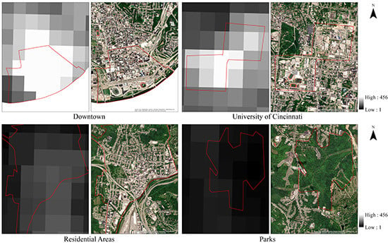
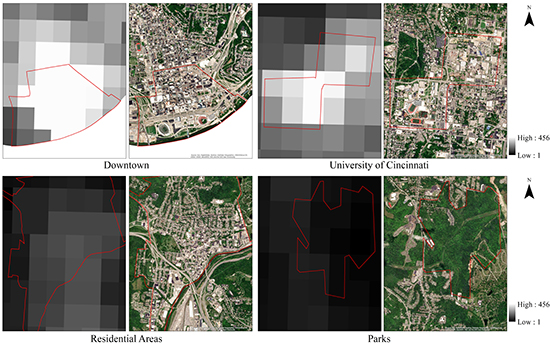
The nightlight satellite data can measure several aspects of the city. First, nightlight satellite data can measure socioeconomic developments, such as gross domestic product [25,26,27,28], carbon emission [25,29,30,31], electricity consumption [32,33,34,35], house vacancy [36], and population study [37,38,39]. Second, nightlight satellite data can measure urban areas in cities. For instance, nightlight satellite data can be applied to investigate urban densities, urban land use, urban expansions, urban spatial clusters, and urban boundaries [40,41,42,43,44,45,46,47,48,49,50,51]. Additionally, nightlight satellite data can measure urban areas inside the city. Figure 1 shows that different types of urban areas in Cincinnati and their corresponding nightlight satellite images in 2012. Except for the University of Cincinnati (UC) which is also bright (UC does not turn off exterior lights at night), Central Business District (CBD) is much brighter than residential areas, industrial areas, and other non-urban areas. It is because roads in CBD are denser than other urban areas such as residential areas in the same city. With the denser and brighter street lights, CBD is brighter, that is, values of nightlight satellite pixels in CBD are also higher than those of other urban areas. Additionally, Figure 1 shows that nightlight satellite pixels in non-urban areas like green areas have lower pixel values than urban areas. Typically, it is because the recorded radiance of nightlight satellite pixels in green areas is far lower than that in urban areas. Since nightlight satellite data can measure socioeconomic developments and urban constructions, this data is a suitable source to measure composite edges that combine both physical edges (changes of urban constructions) and social edges (changes of socioeconomic developments) in a city.
Since nightlight satellite data is the raster data like the pixel grid, the sharp level of composite edges measured by this data is based on the level of changes from a nightlight cell to its neighbors. Table 1 describes some examples of areas where the sharp level of composite edges is typically high or low. The sharp level of composite edges can be low in areas where nightlight cells have the same level of values, such as areas within CBD (or residential areas) where values are consistently high (or moderate), or in the areas within parks or rivers where values are consistently low. In contrast, the sharp level can be high (or moderate) in the areas along the edges of CBD (or residential areas) where high or moderate values are surrounded by low values, or in the areas along the edges of parks or rivers where low values are surrounded by moderate values.
2. Research Questions and Conceptual Framework
To assess the impact of composite edges measured by nightlight satellite data, this study focuses on street robbery and burglary. These two types of crimes are considered for two reasons. First, both street robbery and burglary belong to property crimes. Street robbery means the theft of property in an outdoor, noncommercial location [61]. Burglary means trespassing and theft into residential settings (i.e., a building or automobile) [62]. Thus, both street robbery and burglary are related to socioeconomic developments that nightlight satellite data can capture. Second, street robbery occurs on the streets while burglary occurs inside buildings, both of which are associated with urban infrastructures that nightlight satellite data can capture.
How do composite edges measured by nightlight satellite data affect street robbery and burglary? To answer the question effectively, this study applies the crime pattern theory and the social disorganization theory as the theoretical foundation. The crime pattern theory is applied since edges are key concepts in this theory. The social disorganization theory accounts for other characteristics in addition to edges. The social disorganization theory is selected because it interprets the rate of offenders at the neighborhood level [17], emphasizes the impact of socioeconomic characteristics of local social neighborhoods [63], and focus on the geographical distribution of offender residence [64]. This theory focus on the social disorganization—the incapability of a social unit to keep effective social control, realize common values, and solve long-term problems [65,66,67]. In the social disorganization theory, residential mobility, ethnic heterogeneity, and socioeconomic disadvantage contribute to the increase in the rate of delinquents [68,69,70]. Specifically, a socially disorganized geographic unit characterized by high residential instability, high ethnic heterogeneity, and severe socioeconomic disadvantage (low socioeconomic status) is preferred by street robbery and burglary.
This study estimates a series of negative binomial regression models to reveal the relationship between the tract environment and street robbery/burglary (Figure 2). One scenario is considered in the models: Composite edges can affect street robbery and burglary statistically significantly.
3. Study Area and Data
3.1. Study Area and Crime Data
The study area of this research is the City of Cincinnati (hereafter Cincinnati), a major city in Ohio State, United States. Cincinnati is located in the southwest of Ohio and near the junction of Ohio, Kentucky, and Indiana. According to the FBI report, Cincinnati ranked the 16th most dangerous city in the United States [71] (F.B.I. 2010). The five-year American Community Survey in 2012 showed that there were 324,732 residents in Cincinnati. Additionally, Cincinnati is a high ethnically-diverse city. White occupied the largest number of residents, followed by African-American in 2012. The rental vacancy rate had the largest decrease in 2012 after it peaked in 2006 (12.97%), fallen by 11.30% in 2011 to 6.92% in 2012. The household income was the lowest in 2012 since 2006 according to the Department of Number. The boundary of Cincinnati is downloaded from the Cincinnati Area Geographic Information System (CAGIS, http://cagis.org/Opendata/). Additionally, the 2012 tract-level census data are downloaded from the United States Census Bureau TIGER/Line Shapefiles. This data includes the tract shapefile and demographic information from the five-year ACS data such as population and household income. The 2012 tract-level demographic and economic data released by census bureau are from 2008–2012 five-year ACS data. The typical census data in USA is not available for 2012 since it is collected in every ten years (i.e., 2000 and 2010). Boundaries of census tracts are generally defined by permanent, visible features, such as streets and roads according to the geographic areas reference manual by US Census Bureau. Some of this demographic information is applied as control variables in this research. Since some tracts extend beyond the boundary of Cincinnati, tracts which have caused large noticeable discrepancies are erased. After removing these tracts, there are 114 tracts in Cincinnati in 2012.
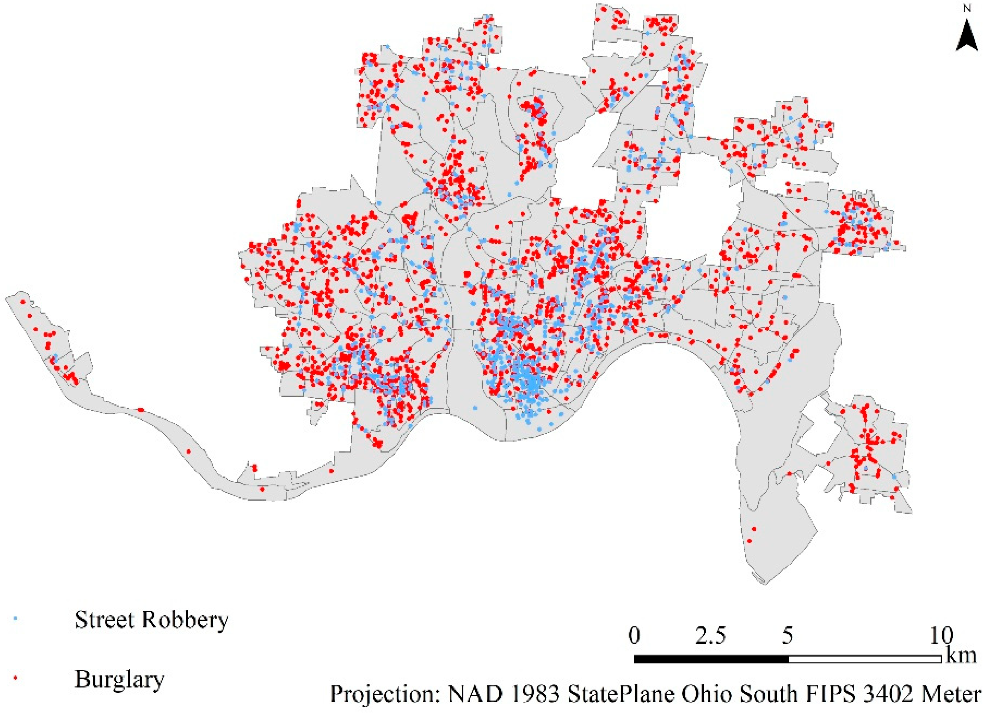
Crime data in Cincinnati in 2012 is provided by the Cincinnati Police Department. There are 36770 geocoded crime incidents reported between January 2012 and December 2012. These crime records include the type of crimes, address, report time, location code such as “street”, “residential facility”, etc. This study selects street robbery data by the type of crime “robbery” and the location code “street”, and burglary data by the type of crime “burglary”. The crime data of this research includes 1050 incidents for street robberies and 3384 incidents for burglaries (Figure 3). Crime data of both street robbery and burglary are aggregated to the tract level. There are 14 tracts that did not witness any street robbery or burglary in 2012.
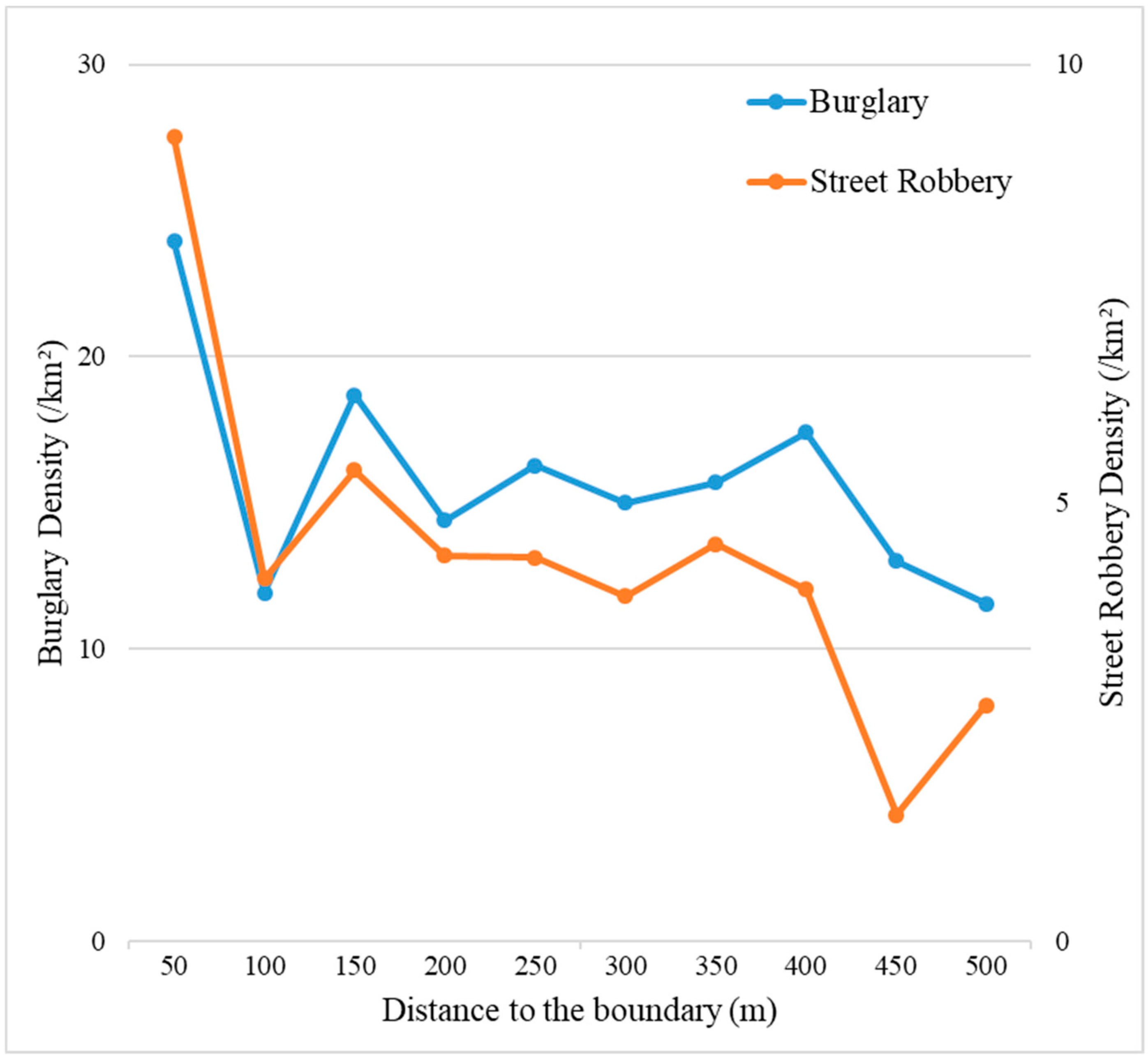
Previous studies investigated the patterns of crimes on spatial boundaries through the proximity analysis [20,22,23]. They found that the curve of the crime density has the distance decay effect: The crime density peaks on or near the edge but drops rapidly and then keeps stable when moving away from the edge. This study applies the same approach to investigate whether the patterns of street robbery or burglary on boundaries of tracts in Cincinnati have the same decay pattern as previous research. The crime density is calculated by dividing the amount of street robbery or burglary by the area of this region for every 50-m increment. Figure 4 shows that burglary and street robbery have a similar crime pattern: As the distance from the tract boundary increases, the crime densities of both street robbery and burglary decrease sharply, and then reach relatively stability. The crime density of burglary is nearly three times the crime density of street robbery because incidents of burglary are three times as many as incidents of street robbery. Both street robbery and burglary in this research match the crime decay pattern in previous studies.
3.2. Nightlight Satellite Data
In a city, nightlight satellite data hardly captures radiated emissions from the earth or the sun but captures lights emitted by the urban constructions or human activities. Sensors on nightlight satellites obtain the radiation intensity of the visible and near-infrared waves emitted by the night surface. They detect the wavelengths at the range of 0.5 to 0.9 μm [72,73]. This range covers most waves in the visible bands (0.38 to 0.74 μm) and a few waves in near-infrared bands (0.74 to 1.4 μm). According to the black-body emission curves of the earth, the emission spectrum of the earth reaches the peak (nearly 17 w·cm−2·sr−1·um−1) in the wavelength of 10 μm and drops closed to 0 w·cm−2·sr−1·um−1 when the wavelength is lower than 5 μm. Therefore, during the nighttime, there is no radiation emission from the sun and the earth, and nightlight satellites capture only visible nightlights from humans.
Nightlight satellite data can be derived from three sources: Defense Meteorological Satellite Program–Operational Linescan System (DMSP-OLS), the Visible Infrared Imaging Radiometer Suite sensor on the Suomi National Polar-orbiting Partnership Satellite (NPP-VIIRS, hereafter VIIRS), and Luojia 1-01. DMSP-OLS releases data from 1992 to 2013 while VIIRS launched in 2012 and Luojia 1-01 launched in June 2018 still work. Sensors on these satellites apply the low-light imaging ability to capture the nightlight data at 7:30 pm (DMSP-OLS), 1:30 am (VIIRS), or 10:00 pm (Luojia 1-01). Luojia 1-01 has the highest spatial resolution (130m) compared with DMSP-OLS (30 arc seconds, nearly 1km) and VIIRS (15 arc seconds, nearly 500m). However, Luojia 1-01 needs the ground control points to make on-orbit geometric calibration whereas the other two satellites have produced products that do not require the geometric calibration [74]. Additionally, unlike DMSP-OLS and VIIRS which have established data that cover most countries in the world, so far Luojia 1-01 only releases data that covers very few regions out of China with a limited time range. Hence, Luojia 1-01 is not considered in this study. Moreover, DMSP-OLS also have limitations. Since DMSP-OLS only records radiance from 10−10 to 10−8 w·cm−2·sr−1·um−1 above the earth’s surface, when the visible and the near-infrared radiance on the earth’s surface such as the bright cores of urban centers and large gas flare is over 10−8 w·cm−2·sr−1·um−1, DMSP-OLS data has saturation. Thus, when applying DMSP-OLS in the urban study, researchers need several approaches to solve saturation, such as the EVI-based method [60]. Since However, VIIRS has a higher spatial resolution and no saturation compared with DMSP-OLS, VIIRS is more superior in mapping nightlight data [75,76]. For example, VIIRS can detect intra-urban variations in brightness in urban cores saturated in the DMSP-OLS imagery. VIIRS can also distinguish small point sources of nightlight at scales approaching 1000 m where DMSP-OLS captures only low luminance background light often indistinguishable from overglow [77]. Therefore, this study uses VIIRS nightlight data.
Nightlight satellite data in this study is the suite of average radiance monthly composites in 2012 from the band Day/Night Band (DNB) in VIIRS. This data is available at National Centers for Environmental Information (NCEI) of National Oceanic and Atmospheric Administration (NOAA) The monthly data has screened out the impact of stray light, lightning, lunar illumination, and cloud-cover before taking the average of the daily data to obtain the monthly data. However, this monthly nightlight satellite data has not been filtered to exclude lights from the aurora, fires, boats, and other temporal lights. Hence, nightlight satellite data in this study has undergone an outlier removal process to filter out fires and other ephemeral lights [36]. Furthermore, since VIIRS nightlight data has a relatively high radiance in winter due to the blocking effect of vegetation canopy [78,79], the nightlight satellite image in December is clearer than other months to show street, industry, and business center. Hence, this study applies VIIRS nightlight imagery in December 2012. We project this data as NAD 1983 State Plane Ohio South coordinates system which is the projection of the study area, and then clip it to the spatial extent of the city of Cincinnati at a spatial resolution of 500 m.
3.3. Edges Defined as Nightlight Gradients
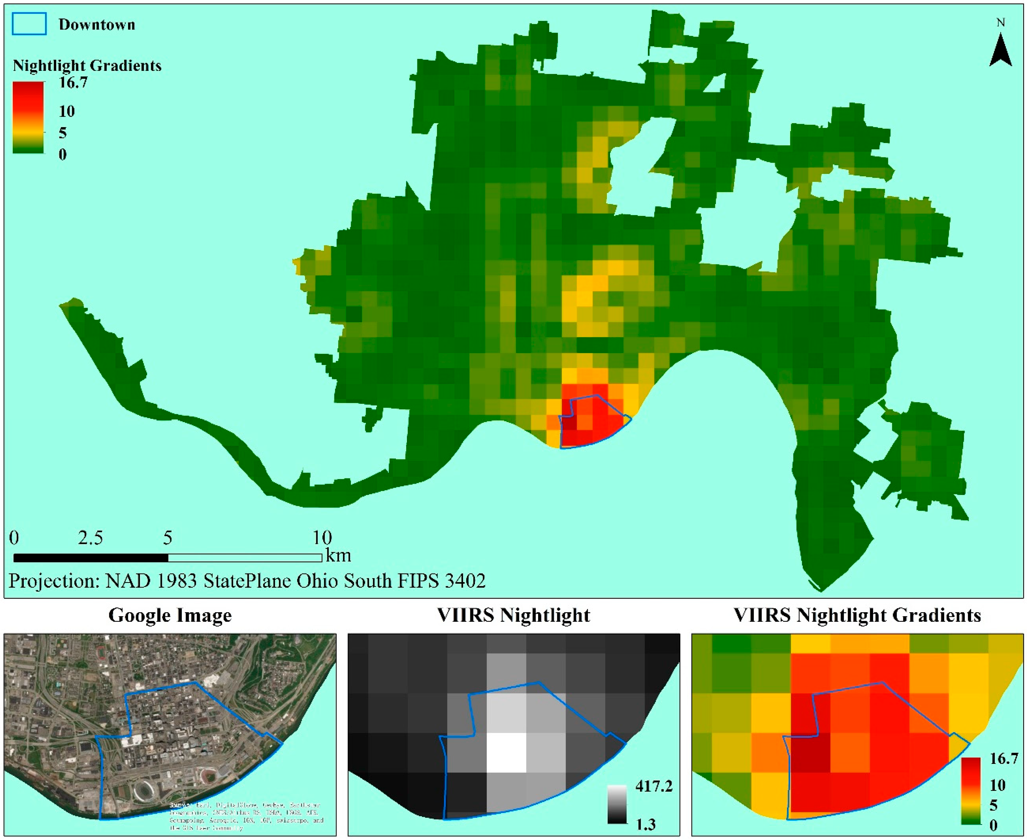
Since edges are defined as the change from one part to another [14,23], this study applies nightlight gradients—gradients of nightlight satellite pixels—to measure composite edges at the tract level in Cincinnati. The nightlight gradients are assigned by the maximum change of values from one nightlight cell to its neighbors measured as the degree level (0°–90°). A higher result value of a cell represents a higher difference to its neighbors. This study applies the Slope function in ArcMap to calculate the nightlight gradients. Figure 5 shows the result of nightlight gradients in Cincinnati. Cells which have high nightlight gradient values (over 10 degrees) are all located in areas surrounding CBD in downtown. The nightlight gradient value of the cell fully inside CBD is not far lower than values of cells in the boundary of CBD because the nightlight value in the center of CBD is far higher than its surrounding neighbor cells. Since the analysis unit in this study is tract, this study introduces a new approach to back up the rationality to aggregate nightlight gradients at the tract level—calculating between variance and within variance of nightlight gradients at the tract level (Table 2). Since between variance is much larger than within variance, the difference of nightlights between tracts is larger than that within tracts. Hence, it is reasonable to aggregate nightlight gradients into the tract level in Cincinnati.
3.4. Operationalization of Variables
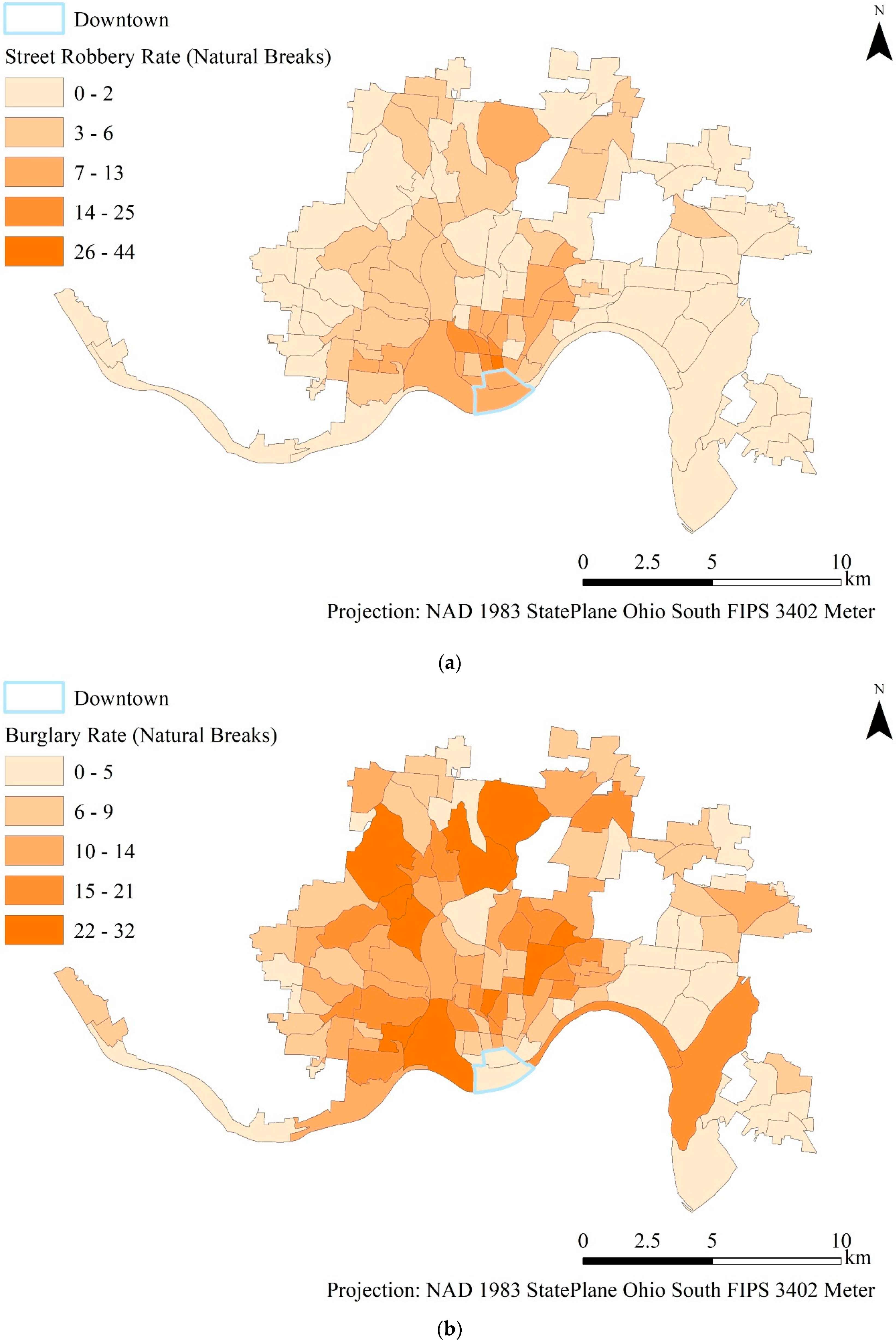
In this study, the tract is chosen as the analysis unit. Data employed in this study include criminal records, variables from census data, and nightlight gradients. Table 3 provides the operationalization of variables, and Table 4 summarizes the descriptive statistic of these variables. The dependent variables are rates of street robbery and burglary at the tract level. Crime rates can be defined as the number of crime incidents by the residential population per 100,000 in a large unit like the county or per 1000 in a small unit like the block group [80,81]. Since the population size of tracts is close to the size of block groups and far smaller than the size of counties, this study defines street robbery rate and burglary rate as the number of crime incidents by the residential population per 1000 at the tract level. The average value of the crime rate of street robbery is 9.32, and the average value of the crime rate of burglary is 30.03. Figure 6 shows the distributions of street robbery rate and burglary rate in Cincinnati. The tracts with high street robbery rates are mainly located in the southern part of Cincinnati, while the tracts with high burglary rates are scattered throughout the city.
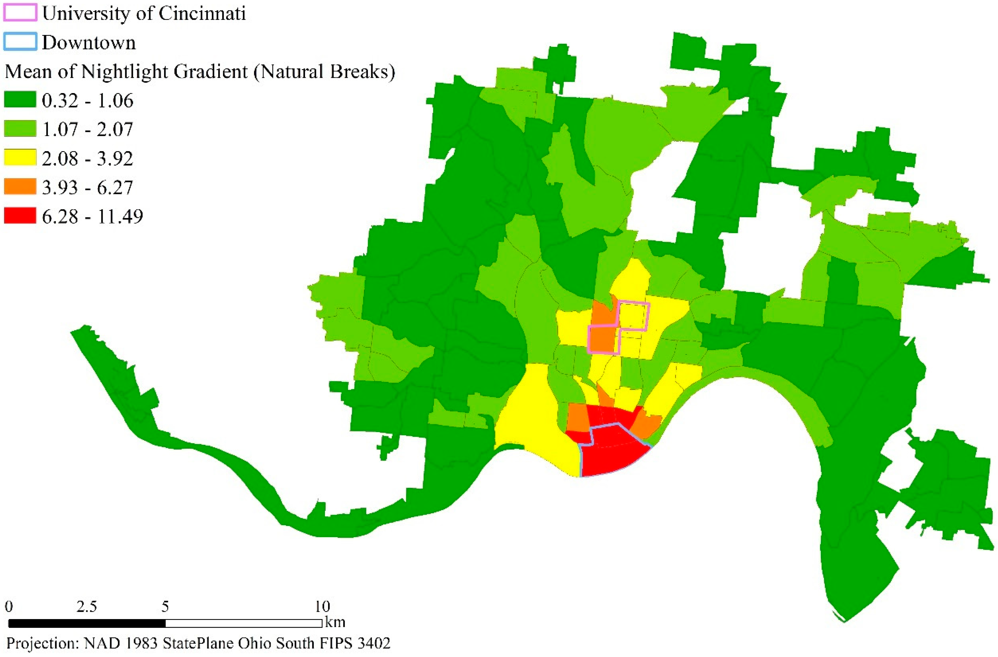
The independent variables include Nightlight Gradient and the control variables. Derived from VIIRS nightlight data, Nightlight Gradient is calculated by the average value of gradients of nightlight satellite pixels at each tract. Since some nightlight gradient cells are not fully inside a tract, this study assigns values of these cells at that tract by multiplying original values with the percentage of these cells that overlap the tract. A tract with a higher value of Nightlight Gradient represents more edges in this tract. Figure 7 shows the distribution of nightlight gradients at the tract level. Tracts with larger values of Nightlight Gradient are located in the downtown and its surrounding areas and UC main campus (the lower left of UC in Figure 7).
To minimize the possibility of obtaining spurious results, the control variables are obtained from the 2012 ACS data in 2012 to measure residential instability, ethnic heterogeneity, and socioeconomic disadvantage in the social disorganization theory. First, the rental rate and the vacant rate are applied to measure residential instability [82]. The rental rate is measured by the percentage of occupied housing units that are renter-occupied at each tract, and the vacant rate is measured by the percentage of housing units that are vacant at each tract. Second, the percentage of the African-American population is used to measure ethnic heterogeneity since both robbery and burglary rates increase as it increases [83]. Third, the low median household income, fewer people with the advanced degree level, and the high young male rate (aging 18–29) can represent socioeconomic disadvantage [68,84]. Since the range of the median household income from the census data is far larger than ranges of the dependent variable and other variables, the effect of this variable for the dependent variable can be weakened. Thus, this study applies the natural logarithm of the median household income. The young male, aged between 18 and 29, is a common variable in past research [85]. The advanced degree level is commonly applied in previous research as well [68,86]. An increase in the percentage of the population with a college degree significantly reduces the robbery rate [83]. This paper uses the percentage of the population with a bachelor’s degree or above in population 25 years and over. Therefore, a tract is expected to have more street robberies and more burglaries if it has higher residential instability (a higher vacancy rate and a higher rental rate), higher ethnic heterogeneity (a higher African-American rate), and higher socioeconomic disadvantage (a lower household income, fewer people with the high level of education, and a higher percentage of young males). Figure 2 summarizes how these control variables are associated with factors in the social disorganization theory.
3.5. Models
The negative binomial regression analysis is employed to investigate the relationship between nightlight gradients and rates of street robbery/burglary. Since Street Robbery Rate and Burglary Rate street robbery rate and burglary rate are both small, distributions of these crime rates do not follow normal or even symmetrical error distributions [80,81]. Both Poisson regression models and negative binomial regression models are appropriate for the count data, but negative binomial regression models can also work for the overdispersed count outcomes [80,87,88,89]. To test whether these two dependent variables are overdispersed, this study calculates the likelihood ratio test of alpha with the negative binomial regression model using Stata 13.0. The alpha coefficients are greater than zero and the likelihood ratio tests for alpha = 0 are significant (Prob > chi2 in Table 5 are all lower than 0.01), which indicates that these two dependent variables are overdispersed. Therefore, this study applies negative binomial regression models. The probability distribution of the negative binomial regression model is shown in Equation (1) where y is the non-negative integer, λ is the mathematical expectation of Y, and τ is a fuzzy parameter representing overdispersed. λ and τ are larger than 0.
Additionally, to test how Nightlight Gradient improves the performance of models to fit street robbery and burglary, this study also applies the negative binomial regression models that exclude Nightlight Gradient. Hence, with the use of the same control variables, there are four negative binomial regression models in this study. In Model 1, the dependent variable is Street Robbery Rate, and the independent variables are only control variables. In Model 2, the dependent variable is Street Robbery Rate, and the independent variables include Nightlight Gradient and control variables; In Model 3, the dependent variable is Burglary Rate, and the independent variables are only control variables. In Model 4, the dependent variable is Burglary Rate, and the independent variables include Nightlight Gradient and control variables. Before running the model, this study applies IBM SPSS Statistic 25 to calculate the variance inflation factors (VIF) of these independent variables to check the collinearity. The VIF values of variables are far below 10 (Table 4), so there is no evidence of collinearity problem. This study uses IBM SPSS Statistic 25 to estimate these four negative binomial regression models.
This study uses the Akaike Information Criterion (AIC) and Incident Rate Ratios (IRRs) to evaluate the fitness of the models. The AIC is an estimator of the quality of each model relative to each of the other models [87]. A smaller AIC value represents better fitness. The IRRs, calculated by exponentiating the coefficient of a model, interpret the effects of independent variables on the dependent variable. An IRR represents a percentage change in the dependent variable per one-unit increase in an independent variable [90]. IRRs larger than 1 indicate positive effects whereas IRRs lower than 1 indicate negative effects. Furthermore, this study applies the 2013 and 2014 data in Cincinnati to validate the impact of composite edges by VIIRS nightlight data.
4. Results
Table 5 summarizes the results of the four negative binomial regression models. The fact that AIC values in Model 2 and Model 4 are lower than those in Model 1 and Model 3 respectively suggests that nightlight gradients consistently improve the negative binomial regression models for both the street robbery rate and the burglary rate. The IRRs in Table 5 show that nightlight gradients in Model 2 and Model 4 make a positive impact on Street Robbery Rate and a negative impact on Burglary Rate, both of which are statistically significant under the alpha level of 0.05. It means that a higher average value of nightlight gradients in a tract increases the street robbery rate but decreases the burglary rate. Since gradients of nightlight pixels represent composite edges—the change from areas with more urban constructions and higher socioeconomic developments to areas with less urban constructions and lower socioeconomic developments, this result also interprets that composite edges measured by VIIRS nightlight data affect both street robbery and burglary statistically significantly.
In each model, at least half of the control variables are statistically significant under the alpha level of 0.05. Vacancy Rate and Rental Rate make a positive impact on crime rates except for Rental Rate in Model 3. It represents that a tract with higher residential instability has higher rates of street robbery and burglary. African-American Rate makes a positive impact on crime rates in all models, so a tract with higher ethnic heterogeneity is associated with a higher rate of street robbery and burglary. The negative impact of Advanced Degree Level and the positive impact of Young Male Rate in all models, and the negative impact of Household Income (Log) in Model 3 and Model 4, demonstrate the contribution of socioeconomic disadvantage to occurrence of street robbery and burglary. In short, except Rental Rate in Model 3 and Household Income (Log) in Model 1 and Model 2, the impact of control variables on the street robbery and burglary replicate the results from previous research that crimes prefer a tract with higher residential instability, higher ethnic heterogeneity, and higher socioeconomic disadvantage [68,69,70].
For the validation of the model, the 2013 and 2014 nightlight data together with the corresponding control variables are used to verify the fitness of the models. As is shown in Table 6, IRRs of Nightlight Gradient are relatively stable and Nightlight Gradient consistently makes positive impacts (IRR > 1) on models of street robbery and negative impacts (IRR < 1) on models of burglary. The AIC values remain relatively stable for all three years. Additionally, in a parenthesis of Table 6, the first value is the AIC value before adding Nightlight Gradient, and the second value is the AIC value after adding Nightlight Gradient for the same dependent variables in the same year. Results of AICs show that Nightlight Gradient consistently improves the performance of models in all three years.
5. Discussion
While this study has underscored the impact of composite edge effects derived VIIRS nightlight data in modeling crime at the tract level, the relatively low spatial resolution of 500m makes it unsuitable for smaller units such as census block groups. Fortunately Wuhan University has released Luojia 1-01 nightlight imageries with a high resolution of 130 m, which can be applied to block groups or even blocks.
Although there are data sources such as census data and land use data that can also be applied to measure edges, nightlight satellite data still represents an attractive option. First, compared with census variables and land use data, nightlight satellite data can directly measure composite edges. Though land use data and census variables can measure physical edges and social edges respectively, it is hard to combine them to measure composite edges. It is because land use data are the category variables and census variables are the continuous variables. Additionally, so far no research provides the theoretical support for deciding the weights of each variable to measure composite edges. However, nightlight satellite data can directly capture the combination of physical edges (changes of urban constructions) and social edges (changes of socioeconomic developments). Second, nightlight satellite data can apply the measure of edges to geographic units and statistical analysis. Since values of land use data are category instead of continuous, scholars mainly used the proximity analysis to measure the impact of edges where different types of land use adjoin on levels of crime [22,23]. However, values of nightlight satellite data are countable, and thus nightlight satellite data can be aggregated to geographic units and work as a continuous variable in statistical models. Third, nightlight satellite data has a higher time resolution than land use data which does not update frequently. For example, the latest land use data in the United States that the public can access is established in 2011, while nightlight satellite data updates yearly or monthly.
Previous studies have specified that more edges contribute to more crimes [1,20,24,57]. This is recognized by the positive impact (IRR > 1) of nightlight gradients on the street robbery rate in this study. Nevertheless, the negative impact (IRR < 1) of nightlight gradients on the burglary rate shows a contradictive conclusion. The different impacts may be explained by the typical location of these two crimes and the local characteristics of nightlights. Street robbery occurs on the streets, so areas with denser streets tend to have more street robberies. Since street lights on streets still work at 1:30 am when the VIIRS satellite captures nightlight, nightlight satellite pixels covering more streets have higher values than pixels with fewer or no streets. Therefore, nightlight gradient values of cells with more streets surrounded by cells with fewer streets can be large, which represents that the sharp level of composite edges is high. This means that composite edges measured by nightlight satellite data are positively related to street robbery. Therefore, tracts with sharper composite edges should have more street robberies. In contrast to street robbery, according to the locational code of the burglary data, 3340 out of 3384 burglary incidents occurred within family zones or residential facilities. Nightlight gradients are low within residential areas but moderate along the edges (Table 1). Therefore, composite edges measured by nightlight satellite data are negatively related to burglary. Therefore, tracts with sharper composite edges should have less burglaries.
Besides the tract level, this study has also explored the effect of nightlight gradients on the street robbery rate and the burglary rate at the neighborhood level in Cincinnati. The patterns of street robbery and burglary also show the same distance decay pattern as the one in Figure 4 and as those from previous studies [22,23], and between variance is also much larger than within variance. Using the same control variables at the neighborhood level, we find consistent results as those of tract level. We have also tested the 2013 and 2014 nightlight data, and they yielded consistent results like those of the 2012 data. This confirms that the models are robust across both the neighborhood level and the tract level and time periods.
6. Conclusions
This study represents the first attempt at introducing nightlight satellite data to measure composite edges in the criminology and assesses the impact of edges on different types of crimes. This study applies nightlight gradients—the maximum change from one nightlight satellite pixel to its neighbor pixels—to represent composite edges. With the use of VIIRS nightlight data in December, crime incidents, and the ACS data in 2012, this study demonstrates the effect of composite edges on street robbery and burglary in Cincinnati after controlling residential mobility, ethnic heterogeneity, and socioeconomic disadvantage. Results of AICs in the negative binomial regression models reveal that nightlight gradients consistently improve the fitness of models of street robbery and burglary. Further, nightlight gradients affect the street robbery rate positively (IRR > 1) and the burglary rate (IRR < 1) negatively, both of which are statistically significant under the alpha level of 0.05. This study also applies the 2013 and 2014 VIIRS nightlight data to validate the impact of composite edges. With the corresponding control variables, the 2013 and 2014 nightlight data yielded consistent results like those of the 2012 data based on AICs and IRRs. The different effects of nightlight gradients on street robbery and burglary are attributed to their contrasting spatial distributions. According to the crime data in this study, street robbery occurred on the streets whilst burglary incidents occurred within family zones or residential facilities. The robust performance of models underscores that nightlight gradients are a reasonable measure of composite edges. Since nightlight satellite data is relatively easy to access globe wide, it can play a vital role in modeling crime, especially in areas where quality census data and land use data are not available.
Author Contributions
Conceptualization, H.Z., L.L., and M.L.; data curation, H.Z.; formal analysis, H.Z.; funding acquisition, L.L.; investigation, H.Z.; methodology, H.Z., L.L., M.L., and B.Y.; resources, H.Z.; supervision, L.L., M.L., B.Y. and Z.W.; validation, H.Z., L.L. and M.L.; visualization, H.Z.; writing—original draft, H.Z.; writing—review and editing, H.Z., L.L. and M.L.
Funding
The research was funded by Research Team Program of Natural Science Foundation of Guangdong Province, China (Grant No. 2014A030312010), Key Program of National Natural Science Foundation of China (Grant No. 41531178), National Key R&D Program of China (Grant Nos. 2018YFB0505500, 2018YFB0505503) and Key Project of Science and Technology Program of Guangzhou City, China (Grant No. 201804020016).
Acknowledgments
We sincerely appreciate anonymous reviewers for their suggestions to improve the quality of this paper.
Conflicts of Interest
The authors declare no conflict of interest.
References
- Brantingham, P.L.; Brantingham, P.J. Residential burglary and urban form. Urban Stud. 1975, 12, 273–284. [Google Scholar] [CrossRef]
- Brantingham, P.J.; Brantingham, P.L. Housing patterns and burglary in a medium-sized American city. Crim. Justice Plan. 1977, 63–74. Available online: https://www.ncjrs.gov/App/Publications/abstract.aspx?ID=44979 (accessed on 25 August 2019).
- Brantingham, P.; Brantingham, P. Notes on the geometry of crime. Environ. Criminol. 1981, 13, 27–53. [Google Scholar]
- Duffala, D.C. Convenience stores, armed robbery, and physical environmental features. Am. Behav. Sci. 1976, 20, 227–245. [Google Scholar] [CrossRef]
- Eck, J.; Weisburd, D.L. Crime places in crime theory. Crime Place Crime Prev. Stud. 2015, 4, 1–33. [Google Scholar]
- Hunter, R.D. Environmental characteristics of convenience store robberies in the state of Florida. In Proceedings of the Annual Meeting of the American Society of Criminology. 1988. Available online: https://www.asc41.com/History.html (accessed on 25 July 2019).
- Rengert, G.F. Burglary in Philadelphia: A critique of an opportunity structure model. Environ. Criminol. 1981, 189–201. Available online: https://www.mendeley.com/catalogue/burglary-philadelphia/ (accessed on 25 August 2019).
- LeBeau, J.L. The methods and measures of centrography and the spatial dynamics of rape. J. Quant. Criminol. 1987, 3, 125–141. [Google Scholar] [CrossRef]
- Mayhew, P.; Britain, G. Crime as Opportunity; HM Stationery Office: London, UK, 1976; Volume 34. [Google Scholar]
- Rengert, G. Theory and practice in urban police response. In Crime: A Spatial Perspective; Columbia University Press: New York, NY, USA, 1980; pp. 276–289. [Google Scholar]
- Stoks, F.G. Assessing urban public space environments for danger of violent crime-especially rape. In Proceedings of the Conference on People and Physical Environment Research. 1983, pp. 331–343. Available online: https://elibrary.ru/item.asp?id=7366133 (accessed on 25 July 2019).
- Jeffery, C.R. An integrated theory of crime and criminal behavior. J. Crim. Law Criminol. Police Sci. 1958, 49, 533. [Google Scholar] [CrossRef]
- Bernasco, W.; Block, R. Robberies in Chicago: A block-level analysis of the influence of crime generators, crime attractors, and offender anchor points. J. Res. Crime Delinq. 2011, 48, 33–57. [Google Scholar] [CrossRef]
- Brantingham, P.L.; Brantingham, P.J. Nodes, paths and edges: Considerations on the complexity of crime and the physical environment. J. Environ. Psychol. 1993, 13, 3–28. [Google Scholar] [CrossRef]
- Brantingham, P.; Brantmgham, P. Criminality of place. Eur. J. Crim. Policy Res. 1995, 3, 5–26. [Google Scholar] [CrossRef]
- Cohen, L.E.; Felson, M. Social change and crime rate trends: A routine activity approach. Am. Sociol. Rev. 1979, 588–608. [Google Scholar] [CrossRef]
- Herbert, D.T.; Hyde, S.W. Environmental Criminology: Testing Some Area Hypotheses. Trans. Inst. Br. Geogr. 1985, 10, 259–274. [Google Scholar] [CrossRef]
- Suttles, G.D. The Social Order of the Slum: Ethnicity and Territory in the Inner City; University of Chicago Press: Chicago, IL, USA, 1968. [Google Scholar]
- Brantingham, P.L.; Brantingham, P.J.; Vajihollahi, M.; Wuschke, K. Crime Analysis at Multiple Scales of Aggregation: A Topological Approach; Springer: New York, NY, USA, 2009. [Google Scholar]
- Kim, Y.-A.; Hipp, J.R. Physical boundaries and city boundaries: Consequences for crime patterns on street segments? Crime Delinq. 2018, 64, 227–254. [Google Scholar] [CrossRef]
- Legewie, J. Living on the edge: Neighborhood boundaries and the spatial dynamics of violent crime. Demography 2018, 55, 1957–1977. [Google Scholar] [CrossRef] [PubMed]
- Song, J.; Andresen, M.A.; Brantingham, P.L.; Spicer, V. Crime on the edges: Patterns of crime and land use change. Cartogr. Geogr. Inf. Sci. 2017, 44, 51–61. [Google Scholar] [CrossRef]
- Song, J.; Spicer, V.; Brantingham, P. The edge effect: Exploring high crime zones near residential neighborhoods. In Proceedings of the 2013 IEEE International Conference on Intelligence and Security Informatics, Seattle, WA, USA, 4–7 June 2013. [Google Scholar]
- Davison, E.L.; Smith, W.R. The relationship between crime and urban location in Raleigh, North Carolina. 2002. Available online: http://www.ncsociology.org/beth9.htm (accessed on 26 July 2019).
- Doll, C.N.; Muller, J.-P.; Morley, J.G. Mapping regional economic activity from night-time light satellite imagery. Ecol. Econ. 2006, 57, 75–92. [Google Scholar] [CrossRef]
- Ghosh, T.; L Powell, R.; D Elvidge, C.; E Baugh, K.; C Sutton, P.; Anderson, S. Shedding light on the global distribution of economic activity. Open Geogr. J. 2010, 3. [Google Scholar] [CrossRef]
- Proville, J.; Zavala-Araiza, D.; Wagner, G. Night-time lights: A global, long term look at links to socio-economic trends. PLoS ONE 2017, 12, e0174610. [Google Scholar] [CrossRef] [PubMed]
- Sutton, P.C.; Elvidge, C.D.; Ghosh, T. Estimation of Gross Domestic Product at Sub-National Scales using Nighttime Satellite Imagery. Int. J. Ecol. Econ. Stat. 2017, 8, 5–27. [Google Scholar]
- Doll, C.H.; Muller, J.-P.; Elvidge, C.D. Night-time imagery as a tool for global mapping of socioeconomic parameters and greenhouse gas emissions. Ambio A J. Hum. Environ. 2000, 29, 157–163. [Google Scholar] [CrossRef]
- Ghosh, T.; Elvidge, C.D.; Sutton, P.C.; Baugh, K.E.; Ziskin, D.; Tuttle, B.T. Creating a global grid of distributed fossil fuel CO2 emissions from nighttime satellite imagery. Energies 2010, 3, 1895–1913. [Google Scholar] [CrossRef]
- Raupach, M.; Rayner, P.; Paget, M. Regional variations in spatial structure of nightlights, population density and fossil-fuel CO2 emissions. Energy Policy 2010, 38, 4756–4764. [Google Scholar] [CrossRef]
- Chand, T.K.; Badarinath, K.; Elvidge, C.; Tuttle, B. Spatial characterization of electrical power consumption patterns over India using temporal DMSP-OLS night-time satellite data. Int. J. Remote Sens. 2009, 30, 647–661. [Google Scholar] [CrossRef]
- He, C.; Ma, Q.; Liu, Z.; Zhang, Q. Modeling the spatiotemporal dynamics of electric power consumption in Mainland China using saturation-corrected DMSP/OLS nighttime stable light data. Int. J. Digit. Earth 2014, 7, 993–1014. [Google Scholar] [CrossRef]
- Shi, K.; Yu, B.; Huang, Y.; Hu, Y.; Yin, B.; Chen, Z.; Chen, L.; Wu, J. Evaluating the ability of NPP-VIIRS nighttime light data to estimate the gross domestic product and the electric power consumption of China at multiple scales: A comparison with DMSP-OLS data. Remote Sens. 2014, 6, 1705–1724. [Google Scholar] [CrossRef]
- Townsend, A.C.; Bruce, D.A. The use of night-time lights satellite imagery as a measure of Australia’s regional electricity consumption and population distribution. Int. J. Remote Sens. 2010, 31, 4459–4480. [Google Scholar] [CrossRef]
- Chen, Z.; Yu, B.; Hu, Y.; Huang, C.; Shi, K.; Wu, J. Estimating house vacancy rate in metropolitan areas using NPP-VIIRS nighttime light composite data. IEEE J. Sel. Top. Appl. Earth Obs. Remote Sens. 2015, 8, 2188–2197. [Google Scholar] [CrossRef]
- Elvidge, C.D.; Baugh, K.E.; Anderson, S.J.; Sutton, P.C.; Ghosh, T. The Night Light Development Index (NLDI): A spatially explicit measure of human development from satellite data. Soc. Geogr. 2012, 7, 23–35. [Google Scholar] [CrossRef]
- Sutton, P. Modeling population density with night-time satellite imagery and GIS. Comput. Environ. Urban Syst. 1997, 21, 227–244. [Google Scholar] [CrossRef]
- Sutton, P.; Roberts, D.; Elvidge, C.; Meij, H. A comparison of nighttime satellite imagery and population density for the continental United States. Photogramm. Eng. Remote Sens. 1997, 63, 1303–1313. [Google Scholar]
- Ma, T.; Zhou, Y.; Wang, Y.; Zhou, C.; Haynie, S.; Xu, T. Diverse relationships between Suomi-NPP VIIRS night-time light and multi-scale socioeconomic activity. Remote Sens. Lett. 2014, 5, 652–661. [Google Scholar] [CrossRef]
- Dou, Y.; Liu, Z.; He, C.; Yue, H. Urban land extraction using VIIRS nighttime light data: An evaluation of three popular methods. Remote Sens. 2017, 9, 175. [Google Scholar] [CrossRef]
- Elvidge, C.D.; Safran, J.; Tuttle, B.; Sutton, P.; Cinzano, P.; Pettit, D.; Arvesen, J.; Small, C. Potential for global mapping of development via a nightsat mission. GeoJournal 2007, 69, 45–53. [Google Scholar] [CrossRef]
- Henderson, M.; Yeh, E.T.; Gong, P.; Elvidge, C.; Baugh, K. Validation of urban boundaries derived from global night-time satellite imagery. Int. J. Remote Sens. 2003, 24, 595–609. [Google Scholar] [CrossRef]
- Imhoff, M.L.; Lawrence, W.T.; Elvidge, C.D.; Paul, T.; Levine, E.; Privalsky, M.V.; Brown, V. Using nighttime DMSP/OLS images of city lights to estimate the impact of urban land use on soil resources in the United States. Remote Sens. Environ. 1997, 59, 105–117. [Google Scholar] [CrossRef]
- Li, X.; Zhao, L.; Li, D.; Xu, H. Mapping urban extent using Luojia 1-01 nighttime light imagery. Sensors 2018, 18, 3665. [Google Scholar] [CrossRef] [PubMed]
- Liu, Z.; He, C.; Zhang, Q.; Huang, Q.; Yang, Y. Extracting the dynamics of urban expansion in China using DMSP-OLS nighttime light data from 1992 to 2008. Landsc. Urban Plan. 2012, 106, 62–72. [Google Scholar] [CrossRef]
- Lo, C. Urban indicators of china from radiance-calibrated digital dmsp-ols nighttime images. Ann. Assoc. Am. Geogr. 2002, 92, 225–240. [Google Scholar] [CrossRef]
- McDonald, R.I.; Kareiva, P.; Forman, R.T. The implications of current and future urbanization for global protected areas and biodiversity conservation. Biol. Conserv. 2008, 141, 1695–1703. [Google Scholar] [CrossRef]
- Shi, K.; Huang, C.; Yu, B.; Yin, B.; Huang, Y.; Wu, J. Evaluation of NPP-VIIRS night-time light composite data for extracting built-up urban areas. Remote Sens. Lett. 2014, 5, 358–366. [Google Scholar] [CrossRef]
- Wu, J.; Ma, L.; Li, W.; Peng, J.; Liu, H. Dynamics of urban density in china: Estimations based on DMSP/OLS nighttime light data. IEEE J. Sel. Top. Appl. Earth Obs. Remote Sens. 2014, 7, 4266–4275. [Google Scholar] [CrossRef]
- Yu, B.; Shu, S.; Liu, H.; Song, W.; Wu, J.; Wang, L.; Chen, Z. Object-based spatial cluster analysis of urban landscape pattern using nighttime light satellite images: A case study of China. Int. J. Geogr. Inf. Sci. 2014, 28, 2328–2355. [Google Scholar] [CrossRef]
- Brantingham, P.J.; Brantingham, P.L.; Molumby, T. Perceptions of crime in a dreadful enclosure. Ohio J. Sci. 1977, 77, 256–261. [Google Scholar]
- Lynch, K. The Image of the City; The MIT Press: Cambridge, MA, USA, 1960. [Google Scholar]
- Groff, E.R.; Weisburd, D.; Yang, S.-M. Is it important to examine crime trends at a local “micro” level? A longitudinal analysis of street to street variability in crime trajectories. J. Quant. Criminol. 2010, 26, 7–32. [Google Scholar] [CrossRef]
- McCutcheon, J.C.; Weaver, G.S.; Huff-Corzine, L.; Corzine, J.; Burraston, B. Highway robbery: Testing the impact of interstate highways on robbery. Justice Q. 2016, 33, 1292–1310. [Google Scholar] [CrossRef]
- Kimpton, A.; Corcoran, J.; Wickes, R. Greenspace and crime: An analysis of greenspace types, neighboring composition, and the temporal dimensions of crime. J. Res. Crime Delinq. 2017, 54, 303–337. [Google Scholar] [CrossRef]
- Brantingham, P.L.; Brantingham, P.J. A topological technique for regionalization. Environ. Behav. 1978, 10, 335–353. [Google Scholar] [CrossRef]
- Brantingham, P.J.; Tita, G.E.; Short, M.B.; Reid, S.E. The ecology of gang territorial boundaries. Criminology 2012, 50, 851–885. [Google Scholar] [CrossRef]
- Hart, T.C.; Miethe, T.D. Public Bus Stops and the Meso Environment: Understanding the Situational Context of Street Robberies. In Safety and Security in Transit Environments; Springer: New York, NY, USA, 2015; pp. 196–212. [Google Scholar]
- Zhuo, L.; Zhang, X.; Zheng, J.; Tao, H.; Guo, Y. An EVI-based method to reduce saturation of DMSP/OLS nighttime light data. Acta Geogr. Sin. 2015, 70, 1339–1350. [Google Scholar]
- Wright, R.; Jacques, S. Street Robbery: Oxford Bibliographies Online Research Guide; Oxford University Press: Oxford, UK, 2010. [Google Scholar]
- Waller, I.; Okihiro, N.R. Burglary: The Victim and the Public; Centre of Criminology, University of Toronto by University of Toronto Press: Toronto, ON, Canada, 1978. [Google Scholar]
- Shaw, C.R.; McKay, H.D. Juvenile delinquency and urban areas: A study of rates of delinquency in relation to differential characteristics of local communities in American cities (1969). In Classics in Environmental Criminology; CRC Press: Boca Raton, FL, USA, 2010; pp. 103–140. [Google Scholar]
- Weisburd, D.; Groff, E.R.; Yang, S.-M. The Criminology of Place: Street Segments and Our Understanding of the Crime Problem; Oxford University Press: Oxford, UK, 2012. [Google Scholar]
- Bursik Jr, R.J. Social disorganization and theories of crime and delinquency: Problems and prospects. Criminology 1988, 26, 519–552. [Google Scholar] [CrossRef]
- Stafford, M.C. Social Sources of Delinquency: An Appraisal of Analytic Models by Ruth R. Kornhauser. Contemp. Sociol. 1981, 10, 232. [Google Scholar] [CrossRef]
- Kubrin, C.E.; Weitzer, R. New directions in social disorganization theory. J. Res. Crime Delinq. 2003, 40, 374–402. [Google Scholar] [CrossRef]
- Liu, L.; Feng, J.; Ren, F.; Xiao, L. Examining the relationship between neighborhood environment and residential locations of juvenile and adult migrant burglars in China. Cities 2018, 82, 10–18. [Google Scholar] [CrossRef]
- Rosenfeld, R.; Fornango, R. The impact of police stops on precinct robbery and burglary rates in New York City, 2003–2010. Justice Q. 2014, 31, 96–122. [Google Scholar] [CrossRef]
- Shaw, C.R.; McKay, H.D. Juvenile Delinquency and Urban Areas; University of Chicago Press: Chicago, IL, USA, 1942. [Google Scholar]
- F.B.I. 2010. Available online: http://os.cqpress.com/citycrime/2011/City_Lo-Hi_2011.pdf (accessed on 25 July 2019).
- Elvidge, C.D.; Erwin, E.H.; Baugh, K.E.; Ziskin, D.; Tuttle, B.T.; Ghosh, T.; Sutton, P.C. Overview of DMSP nightime lights and future possibilities. In Proceedings of the 2009 Joint Urban Remote Sensing Event, Shanghai, China, 20–22 May 2009. [Google Scholar]
- Iona, G.; Butler, J.; Guenther, B.; Graziani, L.; Johnson, E.; Kennedy, B.; Kent, C.; Lambeck, R.; Waluschka, E.; Xiong, X. VIIRS on-orbit optical anomaly: Investigation, analysis, root cause determination and lessons learned. In Proceedings of the Earth Observing Systems XVII, San Diego, CA, USA, 13–16 August 2012. [Google Scholar]
- Zhang, G.; Wang, J.; Jiang, Y.; Zhou, P.; Zhao, Y.; Xu, Y. On-Orbit Geometric Calibration and Validation of Luojia 1-01 Night-Light Satellite. Remote Sens. 2019, 11, 264. [Google Scholar] [CrossRef]
- Elvidge, C.D.; Baugh, K.E.; Zhizhin, M.; Hsu, F.-C. Why VIIRS data are superior to DMSP for mapping nighttime lights. Proc. Asia Pac. Adv. Netw. 2013, 35, 62. [Google Scholar] [CrossRef] [Green Version]
- Li, X.; Xu, H.; Chen, X.; Li, C. Potential of NPP-VIIRS nighttime light imagery for modeling the regional economy of China. Remote Sens. 2013, 5, 3057–3081. [Google Scholar] [CrossRef]
- Small, C.; Elvidge, C.D.; Baugh, K. Mapping urban structure and spatial connectivity with VIIRS and OLS night light imagery. In Proceedings of the Urban Remote Sensing Event, Sao Paulo, Brazil, 21–23 April 2013. [Google Scholar]
- Li, X.; Elvidge, C.; Zhou, Y.; Cao, C.; Warner, T. Remote Sensing of Night-Time Light; Taylor & Francis: Boca Raton, FL, USA, 2017. [Google Scholar]
- Zhao, N.; Hsu, F.-C.; Cao, G.; Samson, E.L. Improving accuracy of economic estimations with VIIRS DNB image products. Int. J. Remote Sens. 2017, 38, 5899–5918. [Google Scholar] [CrossRef]
- Osgood, D.W. Poisson-based regression analysis of aggregate crime rates. J. Quant. Criminol. 2000, 16, 21–43. [Google Scholar] [CrossRef]
- James, A.; Smith, B. There will be blood: Crime rates in shale-rich US counties. J. Environ. Econ. Manag. 2017, 84, 125–152. [Google Scholar] [CrossRef]
- Peterson, R.D.; Krivo, L.J.; Harris, M.A. Disadvantage and neighborhood violent crime: Do local institutions matter? J. Res. Crime Delinq. 2000, 37, 31–63. [Google Scholar] [CrossRef]
- Danzinger, S. Explaining urban crime rates. Criminology 1976, 14, 291. [Google Scholar] [CrossRef]
- Haberman, C.P.; Ratcliffe, J.H. Testing for temporally differentiated relationships among potentially criminogenic places and census block street robbery counts. Criminology 2015, 53, 457–483. [Google Scholar] [CrossRef]
- Braungart, M.M.; Braungart, R.G.; Hoyer, W.J. Age, sex, and social factors in fear of crime. Sociol. Focus 1980, 13, 55–66. [Google Scholar] [CrossRef]
- Gibson, C.L.; Zhao, J.; Lovrich, N.P.; Gaffney, M.J. Social integration, individual perceptions of collective efficacy, and fear of crime in three cities. Justice Q. 2002, 19, 537–564. [Google Scholar] [CrossRef]
- Hilbe, J.M. Negative Binomial Regression; Cambridge University Press: Cambridge, UK, 2011. [Google Scholar]
- Nelder, J.A.; Wedderburn, R.W. Generalized linear models. J. R. Stat. Soc. Ser. A 1972, 135, 370–384. [Google Scholar] [CrossRef]
- McCullagh, P. Generalized Linear Models; Routledge: London, UK, 2019. [Google Scholar]
- Cameron, A.C.; Trivedi, P.K. Regression Analysis of Count Data; Cambridge University Press: Cambridge, UK, 2013; Volume 53. [Google Scholar]
Figure 1.
Nightlight Satellite Data of Cincinnati in 2012 from the band Day/Night Band (DNB) in the Visible Infrared Imaging Radiometer Suite sensor on the Suomi National Polar-Orbiting Partnership Satellite (NPP-VIIRS).
Figure 1.
Nightlight Satellite Data of Cincinnati in 2012 from the band Day/Night Band (DNB) in the Visible Infrared Imaging Radiometer Suite sensor on the Suomi National Polar-Orbiting Partnership Satellite (NPP-VIIRS).

Figure 2.
The relationship between the tract environment and street robbery/burglary.

Figure 3.
Street robbery and burglary in Cincinnati.

Figure 4.
Patterns of street robbery and burglary on boundaries of tracts.

Figure 5.
Distributions of nightlight gradients in Cincinnati and details in/around CBD.

Figure 6.
Distributions of (a) street robbery rate and (b) burglary rate in Cincinnati.

Figure 7.
Nightlight Gradients in Cincinnati.


Table 1.
Examples of areas and their corresponding composite edges measured by nightlight satellite data.
Table 1.
Examples of areas and their corresponding composite edges measured by nightlight satellite data.
| Types of Areas | Nightlight Pixel Values | Sharp Level of Composite Edges |
|---|---|---|
| Areas within CBD or UC | Super high surrounded by high | Moderate |
| Areas within residential areas | Moderate surrounded by moderate | Low |
| Areas within parks or rivers | Low surrounded by low | Low |
| Areas along the edges of CBD or UC | High surrounded by low | High |
| Areas along the edges of residential areas | Moderate surrounded by low | Moderate |
| Areas along the edges of parks or rivers | Low surrounded by moderate | Moderate |
Table 2.
Nightlight Gradients in Cincinnati.
| Analysis Unit | Mean Area (km2) | Between (Variance of Mean) | Within (Mean of Variance) | Unit Amount |
|---|---|---|---|---|
| Tract | 1.80 | 3.91 | 0.81 | 114 |
Table 3.
All variables in negative binomial regression models (N = 114).
| Variables | Description |
|---|---|
| Dependent | All variables are at Tract Level |
| Street Robbery Rate | Counts of reported street robberies per 1000 people |
| Burglary Rate | Counts of reported burglaries per 1000 people |
| Independent | All variables are at Tract Level |
| Nightlight Gradient | Mean of nightlight gradient values |
| Vacancy Rate | Percentage of vacant buildings among all buildings |
| Rental Rate | Percentage of rental buildings among occupied buildings |
| African-American Rate | Percentage of the African-American population among total population |
| Household Income (Log) | The natural logarithm of the median household income |
| Advanced Degree Level | Percentage of population with bachelor’s degree or higher degree among population aged 25 or more |
| Young Male Rate | Percentage of 18 to 29 male among total population |
Table 4.
Descriptive information of variables.
| Variables | Minimum | Maximum | Mean | Standard Deviation | VIF |
|---|---|---|---|---|---|
| Dependent | |||||
| Street Robbery Rate | 0 | 50 | 9.32 | 9.68 | |
| Burglary Rate | 0 | 158 | 30.03 | 24.61 | |
| Independent | |||||
| Nightlight Gradient | 0.32 | 11.48 | 1.75 | 1.98 | 1.78 |
| Vacancy Rate | 0.02 | 0.71 | 0.22 | 0.13 | 2.25 |
| Rental Rate | 0.10 | 1.00 | 0.59 | 0.21 | 4.03 |
| African-American Rate | 0.00 | 0.95 | 0.42 | 0.30 | 2.42 |
| Household Income (Log) | 8.92 | 11.60 | 10.37 | 0.55 | 5.80 |
| Advanced Degree Level | 0.03 | 0.83 | 0.30 | 0.21 | 2.42 |
| Young Male Rate | 0.01 | 0.50 | 0.11 | 0.09 | 1.76 |
Table 5.
Results of negative binomial regression models.
| Variables | Incident Rate Ratios (IRRs) | |||
|---|---|---|---|---|
| Street Robbery Rate | Burglary Rate | |||
| Model 1 | Model 2 | Model 3 | Model 4 | |
| Nightlight Gradient | 1.11 ** | 0.90 *** | ||
| Vacancy Rate | 55.85 *** | 22.82 *** | 1.05 | 2.20 |
| Rental Rate | 13.23 *** | 5.02 * | 0.74 | 1.16 |
| African-American Rate | 2.32 * | 2.14 * | 1.14 | 1.17 |
| Household Income (Log) | 1.39 | 1.04 | 0.53 ** | 0.61 ** |
| Advanced Degree Level | 0.29 * | 0.12 ** | 0.38** | 0.48 * |
| Young Male Rate | 20.60 ** | 21.21 ** | 4.94* | 5.92 ** |
| (Constant) | 0.00 | 0.19 | 9423.42 *** | 1483.40 *** |
| Alpha | 0.20 | 0.17 | 0.10 | 0.08 |
| Prob > = chi2 | 0.00 | 0.00 | 0.00 | 0.00 |
| AIC | 450.10 | 445.77 | 667.33 | 657.93 |
Note: * p < 0.05, ** p < 0.01, *** p < 0.001.
Table 6.
Results of IRR of Nightlight Gradient and AIC reduction in 2012–2014.
| Variables | Street Robbery Rate | Burglary Rate | ||||
|---|---|---|---|---|---|---|
| 2012 | 2013 | 2014 | 2012 | 2013 | 2014 | |
| IRR of Nightlight Gradient | 1.11 ** | 1.41 *** | 1.24 *** | 0.90 *** | 0.88 ** | 0.95 * |
| AIC Reduction | Yes (450.10 > 445.77) | Yes (464.36 > 442.80) | Yes (435.96 > 421.99) | Yes (667.33 > 657.93) | Yes (709.73 > 707.21) | Yes (662.57 > 661.15) |
Note: * p < 0.05, ** p < 0.01, *** p < 0.001. AIC values are shown in the parentheses.
© 2019 by the authors. Licensee MDPI, Basel, Switzerland. This article is an open access article distributed under the terms and conditions of the Creative Commons Attribution (CC BY) license (http://creativecommons.org/licenses/by/4.0/).
Share and Cite
MDPI and ACS Style
Zhou, H.; Liu, L.; Lan, M.; Yang, B.; Wang, Z. Assessing the Impact of Nightlight Gradients on Street Robbery and Burglary in Cincinnati of Ohio State, USA. Remote Sens. 2019, 11, 1958. https://doi.org/10.3390/rs11171958
AMA Style
Zhou H, Liu L, Lan M, Yang B, Wang Z. Assessing the Impact of Nightlight Gradients on Street Robbery and Burglary in Cincinnati of Ohio State, USA. Remote Sensing. 2019; 11(17):1958. https://doi.org/10.3390/rs11171958
Chicago/Turabian StyleZhou, Hanlin, Lin Liu, Minxuan Lan, Bo Yang, and Zengli Wang. 2019. "Assessing the Impact of Nightlight Gradients on Street Robbery and Burglary in Cincinnati of Ohio State, USA" Remote Sensing 11, no. 17: 1958. https://doi.org/10.3390/rs11171958
Note that from the first issue of 2016, this journal uses article numbers instead of page numbers. See further details here.