Article

Coupling an Intercalibration of Radiance-Calibrated Nighttime Light Images and Land Use/Cover Data for Modeling and Analyzing the Distribution of GDP in Guangdong, China

1
Key Laboratory of Marginal Sea Geology, Guangzhou Institute of Geochemistry, Chinese Academy of Sciences, Guangzhou 510640, China
2
University of Chinese Academy of Sciences, Beijing 100089, China
3
School of Geographical Sciences, Guangzhou University, Guangzhou 510006, China
*
Author to whom correspondence should be addressed.
Sustainability 2016, 8(2), 108; https://doi.org/10.3390/su8020108
Submission received: 17 November 2015 / Revised: 18 January 2016 / Accepted: 20 January 2016 / Published: 26 January 2016

Abstract

:
Spatialized GDP data is important for studying the relationships between human activities and environmental changes. Rapid and accurate acquisition of these datasets are therefore a significant area of study. Defense Meteorological Satellite Program/Operational Linescan System (DMSP/OLS) radiance-calibrated nighttime light (RC NTL) images exhibit the potential for providing superior estimates for GDP spatialization, as they are not restricted by the saturated pixels which exist in nighttime stable light (NSL) images. However, the drawback of light overflow is the limited accuracy of GDP estimation, and GDP data estimations based on RC NTL images cannot be directly used for temporal analysis due to a lack of on-board calibration. This study develops an intercalibration method to address the comparability problem. Additionally, NDVI images are used to reduce the light overflow effect. In this way, the secondary and tertiary industry outputs are estimated by using intercalibrated RC NTL images. Primary industry production is estimated by using land use/cover data. Ultimately, four 1 km gridded GDP maps of Guangdong for 2000, 2004, 2006 and 2010 are generated. The verification results of the proposed intercalibration method demonstrate that this method is reasonable and can be effectively implemented. These maps can be used to analyze the distribution and spatiotemporal changes of GDP density in Guangdong.

1. Introduction

With the intensification of research on global change, increasing attention has been paid to the interaction mechanism between human activities and the environment [1]. As the largest developing country, China has undergone a period of rapid development in the last thirty years. During this period, the relationships between human activities (including expansion of urban areas, economies, and populations) and environmental change have gradually intensified, and an increasing number of studies have focused on this problem [2,3]. GDP data is an important index of human economic activities that is utilized in many studies related to regional planning and development, resources and environmental protection, and sustainable development [4]. However, GDP data and natural elements datasets (e.g., climate, soil, and elevation) have been collected separately based on different spatial units. The first type of data is usually provided on the basis of administrative units, and the second type of data is usually available in grid or raster formats. This causes a spatial mismatch between these datasets [5,6]. Thus, rasterizing GDP data has become a core issue in the related literature.
Traditionally, the spatialization of GDP data has been conducted by assuming a uniform distribution across a given administrative unit. However, this average distribution ignores the spatial heterogeneity within spatial units and hence cannot reflect the distribution of actual economic activities. With the development of remote sensing technology in recent years, the land use/cover data [7] and nighttime light (NTL) images [8] have been used to estimate economic activities. Because Operational Linescan System (OLS) sensors have unique low-light sensing capabilities [9,10,11], NTL images on board these sensors can intuitively reflect the economic activities of human beings. Therefore, NTL images [12,13,14,15,16,17] are more commonly used than land use/cover data. Previous studies have demonstrated that DMSP/OLS NTL imagery can be used to develop a statistically significant indicator of economic activities [18,19,20,21]. NTL images have been widely applied for GDP spatialization [15,22,23,24,25]. In spite of this, significant drawbacks hinder further improvements in the application of the NTL imagery. The pixel saturation phenomenon [26] that is always present in urban centers and the problem of light overflow [27] are the major limitations for improving the accuracy of related studies. When NTL images were used for GDP spatial distribution in previous studies, the contribution from the agricultural sector was not fully considered. Generally, studies have distributed agricultural contributions in the darker areas of NTL images. To solve these problems, some saturation corrected methods [17,28,29] and light overflow corrected approaches [27,30,31] have been proposed. Among these approaches, the radiance-calibrated NTL images based on merging three types of gain setting [10,32,33] have relatively better desaturation effect. Furthermore, studies have shown that utilizing the threshold methods to reduce the light overflow effect is feasible. Despite all this research, the correlation between radiance-calibrated NTL imagery and GDP has not been confirmed at the sub-national scale. Additionally, even if GDP spatialization has been carried out for a given year, temporal change analysis cannot be implemented due to a lack of a spatialized GDP time series dataset.
In this study, the radiance-calibrated NTL imagery is chosen over other NTL images because it was not affected by pixel saturation and because we found that it exhibits a strong linear correlation between with Guangdong GDP data at county level. Based on the research of Hsu et al. [33], an intercalibration method established on the invariant region method is developed for Guangdong to address the lack of comparability in the radiance-calibrated NTL time series dataset. According to the negative correlation between the light intensity of NTL imagery and vegetation index [29,34,35], a threshold method based on normalized differential vegetation index (NDVI) is then proposed to decrease the light overflow effect for the intercalibration of radiance-calibrated NTL images. Land use/cover data is selected to estimate the spatial distribution of the primary industry production in Guangdong province. The intercalibration of radiance-calibrated NTL images, which reduced the light overflow effect, is used to estimate the spatial distribution of secondary and tertiary industry outputs in Guangdong province. Finally, we produced four GDP density maps of Guangdong province for 2000, 2004, 2006 and 2010 and analyzed the spatiotemporal variation of GDP density (Figure 1).
Figure 1. Flow chart of research process. Green represents primary data, red represents methods and blue represents results and analysis.
Sustainability 08 00108 g001

2. Study Area, Data, and Pre-Processing
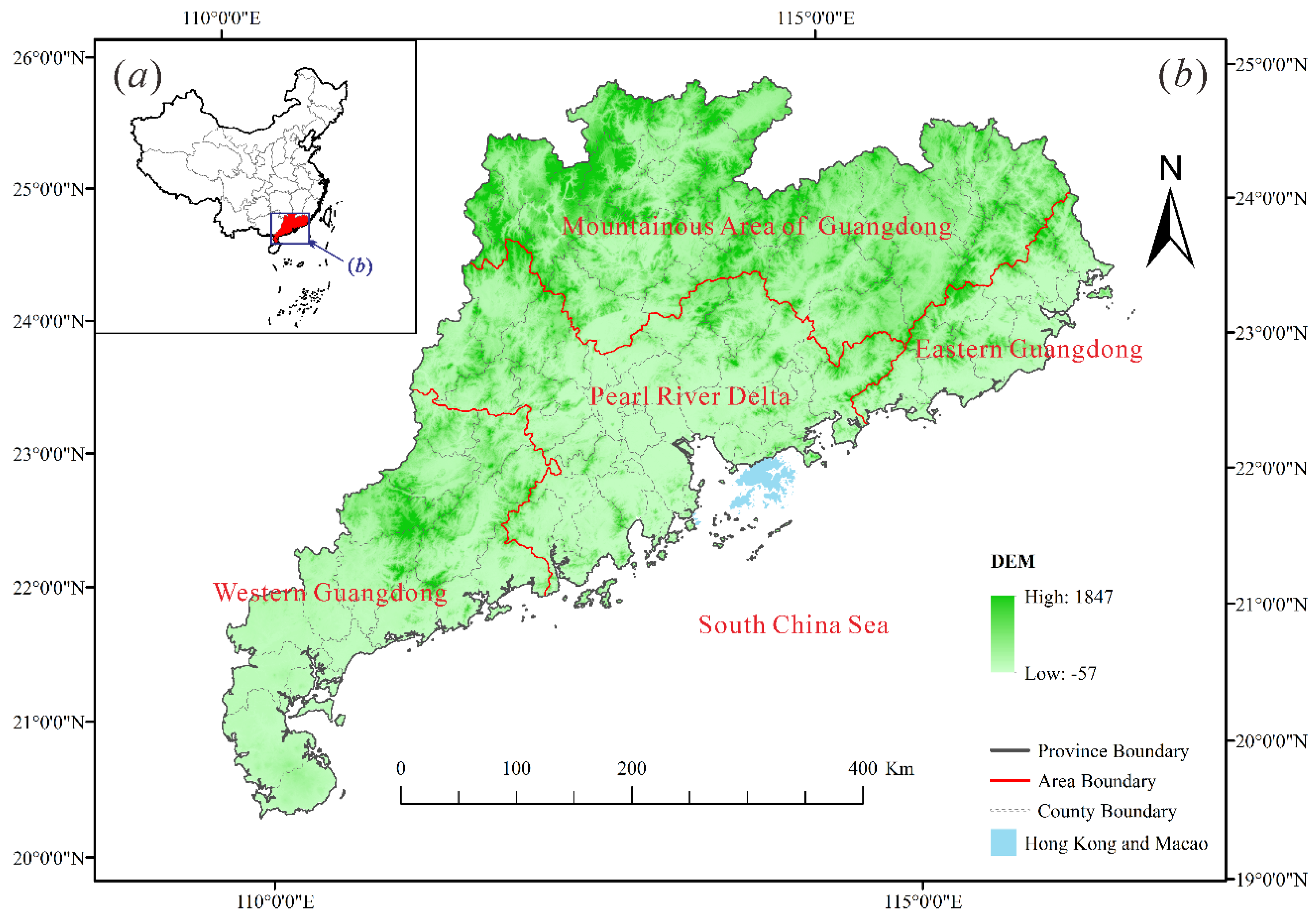
2.1. Study Area

Guangdong province is located in the region within the range of 20°09′ N–25°31′ N and 109°45′ E–117°20′ E in the southernmost part of Mainland China. The province borders the South China Sea to the south and has 4300 km of coastline. The total land area of Guangdong is 179,700 km2, 0.89% of which is islands. The topography of Guangdong is complex with 58.6% of the total land area covered by mountains, which are mostly concentrated in the northern part of the province. Plains and mesas only account for 35.9% of the total land area, and the remaining 5.5% is composed of rivers and lakes. Guangdong province, including 21 cities and 119 counties, can be divided into four areas: the Pearl River delta, eastern Guangdong, western Guangdong and the mountainous area of Guangdong (Figure 2). Since 1989, Guangdong has consistently exhibited the largest GDP among all the mainland provinces of China. According to the China Statistical Yearbook 2010 [36], Guangdong’s GDP accounts for 11.43% of the total GDP of Mainland China. The GDP and GDP per capita of Guangdong are 4547.28 billion CNY and 43,597 CNY, respectively. Regarding the GDP contributions of different industries, secondary and tertiary industries represent 94.97% of the total GDP of Guangdong province.
Figure 2. Location of Guangdong Province, China.
Sustainability 08 00108 g002

2.2. Data and Pre-Processing

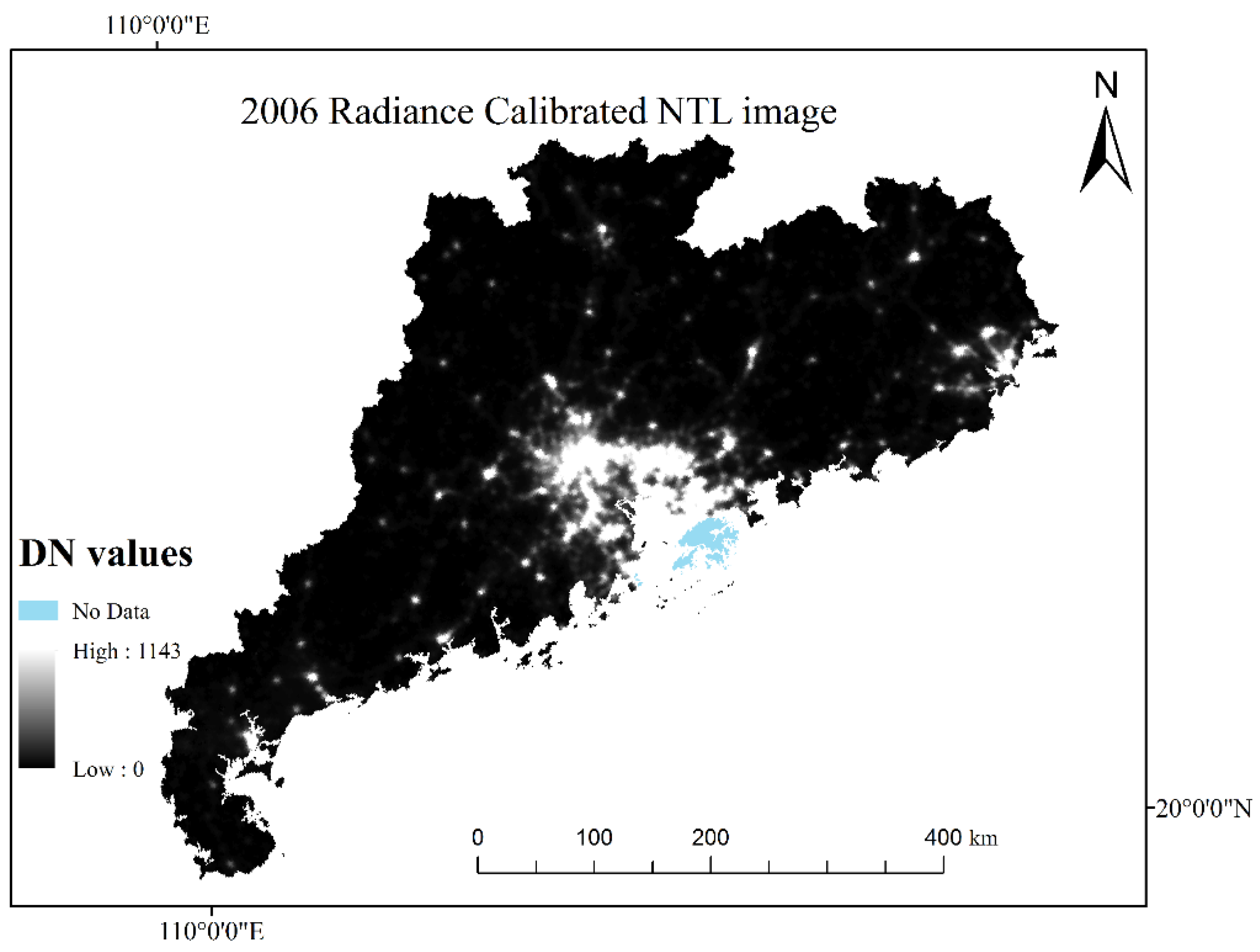
2.2.1. Defense Meteorological Satellite Program/Operational Linescan System (DMSP/OLS) Nighttime Light Image

The DMSP/OLS nighttime light (NTL) images were provided by the National Oceanic and Atmospheric Administration (NOAA)/National Geography Data Center (NGDC) website [37]. There are two types of NTL images. The most commonly used images are the stable light annual average images of the “Global DMSP/OLS Nighttime Lights Time Series” (Version 4). Stable light data covers cities, towns, and other persistent sources of light; background noise, such as fires and moonlit clouds, have been removed from this dataset. Additionally, the NGDC website [37] has released eight “Global Radiance Calibrated Products.” These lights datasets were produced by merging DMSP/OLS data acquired at low gain settings with operational data acquired at high gain settings. The radiance-calibrated NTL images use three stages of gain settings for the DMSP satellite to record nighttime lights with different brightness levels. By merging the images obtained under each gain setting, an extra-large dynamic range is achieved that can fully accommodate bright city lights. These fixed-gain images were further blended with the operationally stable light product to recover additional details in dim areas. Compared with stable light images, the radiance-calibrated images do not include saturated pixels in the bright cores of urban areas and have a greater range of DN values. In this study, 2000, 2004, 2006, 2010, and 2010_2011 radiance-calibrated nighttime light (RC NTL) images were selected. Each NTL image was extracted according to the administrative boundaries of Guangdong province, re-projected to the Lambert Azimuthal Equal Area projection and resampled to a 1 km grid (Figure 3).
Figure 3. DMSP/OLS radiance-calibrated nighttime light image of Guangdong in 2006.
Sustainability 08 00108 g003

2.2.2. Moderate-Resolution Imaging Spectroradiometer Normalized Difference Vegetation Index Data

Terra MODIS 16-day 1 km NDVI composite images (MOD13A2) were downloaded from the National Aeronautics and Space Administration (NASA)/Goddard Space Flight Center (GSFC) website [38]. As a level-3 product, the Terra MODIS 16-day 1 km NDVI products are based on the level-2 daily surface reflectance product (MOD09 series), which provides red and near-infrared surface reflectance that has been corrected for the effects of atmospheric gases, thin cirrus clouds, and aerosols [39]. These products are generated through aggregation of the red (band 1) and near-infrared (band 2) from their native 250 m resolution via the MODIS Gridding and Aggregation Process [40]. To address the angular variations that are inherent to most space-based imaging instruments and to reduce the spatial and temporal discontinuities in the multi-day composites, the MODIS NDVI composites are generated through a constrained view maximum value compositing (CV-MVC) method [41]. In this study, we calculated annual NDVI mean values using multi-temporal NDVI images from 2000, 2004, 2006, and 2010. All of the annual NDVI images were projected into the Lambert Azimuthal Equal Area projection and resampled to a pixel size of 1 km based on a nearest-neighbor resampling algorithm. We then extracted the images based on the administrative boundaries of Guangdong province.

2.2.3. Land Use/Cover Data

Chinese land use/cover dataset with a scale of 1:100,000 was obtained from the Resources and Environment Data Center of the Chinese Academy of Science (RESDC) [42]. This dataset covers five years: 1990, 1995, 2000, 2005 and 2010. The major source of this data is Landsat TM/ETM remote sensing data. These land use/cover data are produced by visual interpretation; the spatial resolution is 1 km [43,44,45]. Land use types include six first-level types which are cultivated land, forest land, grassland, water body, residential areas, and unused land. The dataset also includes 25 second-level types. For the purpose of this research, land use/cover data in 2000, 2005, and 2010 were picked and they all were selected. This data was extracted according to administrative boundaries of Guangdong province and was projected to the Lambert Azimuthal Equal Area projection.

2.2.4. Ancillary Data

The boundaries of the county-level administrative units are based data from the National Geomatics Center of China with a scale of 1:4,000,000. Our study focused only on Guangdong province, and the boundaries of Guangdong were therefore extracted from the Chinese map. Because the statistical data of all the districts under the administrative control of a city were calculated as a single statistic, the number of county-level units in the statistical data was less than in the official reports. Therefore, we adjusted the boundaries of county-level administrative units in Guangdong via ArcGIS 10.1 and ensured it had a consistent number with the statistical data. Guangdong was divided into 82 counties, though not the 119 counties of official standards.
The GDP and other statistical data were obtained from the Guangdong Statistical Yearbook [46], and the Agricultural Statistical Yearbook of Guangdong for the years studied [47].

3. Methods

3.1. Intercalibration of DMSP/OLS Radiance-Calibrated Nighttime Light Time Series Images

DMSP/OLS RC NTL images from different years cannot be compared due to a lack of on-board calibration. To address this problem, many studies employed different intercalibration methods. Among them, only Hsu et al. [33] intercalibrated the RC NTL time series dataset at a global scale. Therefore, an improved intercalibration method was developed for Guangdong based on the method of the Hsu et al. study. This is the first time that this method has been used at the sub-national scale and is the first application of inter-annual correction amongst the RC NTL images. The intercalibration method includes three steps: (1) inter-satellite calibration; (2) inter-annual calibration and (3) inter-annual series correction.

3.1.1. Inter-Satellite Calibration

For this step we used the exact same parameters that were utilized in the study of Hsu et al. [33]. The inter-satellite calibration is carried out before the creation of a single annual image. Therefore, we do not provide further details in this article.

3.1.2. Inter-Annual Calibration

To perform a comparative study between RC NTL images, an invariant region method was applied. This method assumes that stable pixels exist in a series of remote sensing images and that these stable pixels can be extracted to serve as the invariant region. The invariant regions obtained in different phases of remote sensing images processing present a unique transformation relationship. This transformation relationship can be used for intercalibration of a multi-temporal remote sensing dataset [48,49,50]. Elvidge et al. [51] first intercalibrated the global NSL dataset by using the invariant region method. Subsequently, Liu et al. [52] intercalibrated the Chinese NSL dataset via a similar method. The correction results of their studies indicated that this method improved the comparability of the NSL image in the dataset.
For the RC NTL time series images, a similar model was demonstrated in Hsu et al. [33] for comparisons between RC NTL images from 1996 to 2010. The authors chose Los Angeles, USA as the invariant region. The authors chose Los Angeles as it has been a mature metropolis for a long period of time and the light change is negligible. Furthermore, Los Angeles could provide samples with high digital numbers (DNs) from the city center as well as low DNs from the suburban area. Based on these criteria and the location of Guangdong province, Guangzhou or Shenzhen were taken as invariant regions. Although these areas are still rapidly developing, Guangzhou and Shenzhen both have higher DN values than other surrounding cities in the 2000, 2004, 2006, 2010, and 2010_2011 RC NTL images. Both of these regions also have a greater range of DN values than other cities in Guangdong. These characteristics improve the accuracy of the intercalibration. Additionally, only the 2006 RC NTL image derived from the same satellite with its blended stable lights image provides a fair cloud-free coverage. Therefore, the RC NTL image in 2006 was taken as the reference image.
Both Elvidge et al. [51] and Liu et al. [52] proposed a second order polynomial regression to address the curvature in correlation when the DN values approached saturation in the NSL images. However, Hsu et al. [33] developed a linear regression for intercalibration of the RC NTL images. Therefore, the second order polynomial regression analysis and linear regression analysis between the RC NTL images and GDP data were both carried out for Guangdong. The resulting coefficients are shown in the Table 1. According to the coefficients, the second order polynomial regression is superior to the linear regression. The inter-annual calibration model of the RC NTL images was therefore established as Equation (1).
D N i c = a × D N 2 + b × D N + c
where DN is the DN value in the RC NTL images; DNic is the DN value in the inter-annual calibrated RC NTL images; and a, b, and c are coefficients.
Table 1. Coefficient comparison of linear regression and second order polynomial regression.
Satellite_YearR2 (Linear)R2 (Second Order Polynomial)
ShenzhenGuangzhouShenzhenGuangzhou
F12-F15_20000103-200012290.90590.90830.94030.9176
F14_20040118-200412160.91760.95950.95970.9628
F16_20051128-200612241.00001.00001.00001.0000
F16_20100111-201012090.68430.79180.68450.8317
F16_20100111-201107310.90370.93830.93980.9497
For RC NTL images in different years, the city between Guangzhou and Shenzhen which had the higher coefficient value was selected as the invariant region. To ensure the lit pixel is still the lit pixel and is not the negative value after inter-annual calibration, the constant c in Equation 1 was set as 0. Then the model for the inter-annual calibration was changed to Equation (2).
D N i c = a × D N 2 + b × D N
where DN is the DN value in the RC NTL images; DNic is the DN value in the inter-annual calibrated RC NTL images; and a and b are coefficients.

3.1.3. Inter-Annual Series Correction

The inter-annual calibration solves the RC NTL image comparison issue, but the inconsistencies in lit pixels among the multi-year images still persist. These inconsistencies mean that lit pixels change to unlit pixels in the next year at the same geographical locations and that abnormal DN fluctuations appear across different years. Because GDP continuously increased and no natural catastrophes (e.g., earthquake, tsunami, and warfare) occurred in Guangdong during the last thirteen years, we generated the following assumption to filter noise points. The lit pixels detected in an annual NTL image should not disappear in a later year and a lit pixel’s DN value should not be less than the DN value of the lit pixel in the same geographic location the following year. Therefore, we can obtain an inter-annual series correction model for the RC NTL images after inter-annual calibration by following two rules: (1) when a pixel’s DN value is equal to zero in an image, that pixel’s DN value for the previous year at the same geographic position should also be equal to zero, and (2) when a pixel’s DN value is not equal to zero in an image, the pixel’s DN value must be greater than the DN value of the lit pixel in the same geographic position in the previous year. This is described in Equation (3).
D N ( n , i ) = { 0 D N ( n 1 , i ) D N ( n , i ) D N ( n + 1 , i ) = 0 D N ( n + 1 , i ) > 0   and   D N ( n 1 , i ) > D N ( n , i ) otherwise
where DN(n-1,i), DN(n,i), and DN(n+1,i) are the DN values of the i-th lit pixel in the RC NTL image after inter-annual calibration in the (n − 1)-th, the n-th, and (n + 1)-th years, respectively. n = 2000, 2004, 2006, 2010, and 2010_2011.
In this method, the 2010 and 2010_2011 RC NTL images both include the light information of 2010. In both two types of regression analysis, 2010_2011 images have a better relationship with the 2006 RC NTL image than 2010 image. Therefore, the accuracy of inter-annual calibration of the 2010_2011 RC NTL image is superior to the accuracy of inter-annual calibration of the 2010 RC NTL image. However, the 2010_2011 RC NTL image can help improve the 2010 RC NTL image through inter-annual series correction and as a result of the 2010_2011 RC NTL image including some space observations from 2011. Finally, the intercalibrated RC NTL image in 2010 was chosen to represent 2010.

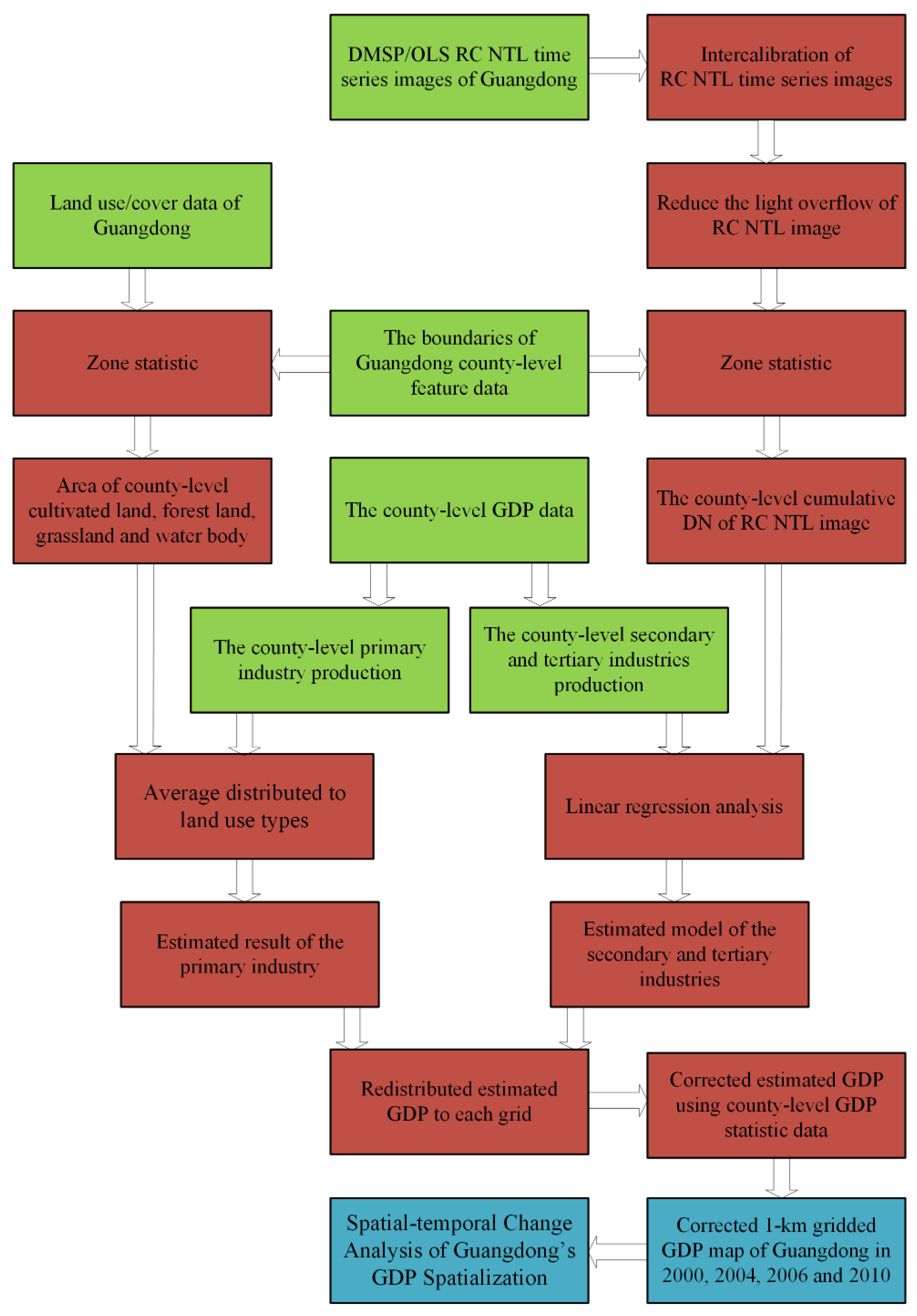
3.2. Estimation of GDP Spatialization by Land Use/Cover Data and RC NTL Imagery

Several GDP spatialization studies [22,24,31] have used land use/cover data to model the primary industry production and DMSP/OLS NTL imagery to simulate secondary and tertiary industry production. This is because land use/cover data can estimate the production of various second-level industry types in the primary industry and NTL imagery cannot reflect production in the rural areas where there are dark areas. In this study, these two types of data were chosen. As the pixel saturation in the NTL data affects the accuracy of the estimated GDP spatialization, the RC NTL images which did not include saturated pixels was selected to estimate the secondary and tertiary industry production. In addition, a NDVI threshold method was utilized to reduce light overflow effect and thereby improve the estimation accuracy of the secondary and tertiary industry production.

3.2.1. Estimation of the Primary Industry Production by Using Land Use/Cover Data

The primary industry production spatialization method equally distributes the second-level industry production (farming, forestry, animal husbandry and fishery) of the primary industry to corresponding land use types in every county. The different land use types represent the corresponding agricultural sectors: dry land and paddy fields are designated as the farmland land type; all types of forest land are designated as the forestry land type; all types of grassland are designated as the animal husbandry land type; bodies of water, including rivers and lakes, are designated as the fishery land type. The statistical primary industry production in Guangdong province for the four second-level industries of agriculture were individually collected from the Agricultural Statistical Yearbook of Guangdong [47] at the county level. For a given county, the pixel-based production for a certain second-level industry is calculated on the basis of the ratio between the second-level industry production and the number of corresponding land use pixels (Equation (4)).
The second-level industry production model as primary industry:
G L i j = g i j × L i j
GLij (i = 1–4) are the production outputs of the farming, forestry, animal husbandry, and fishery primary industries of j-th county, respectively. gij is the average production value of the i-th land use type in this county. Lij are the perspective areas of the i-th land use types (cultivated land, forest land, grassland, and water body) in each county.
Using Equation (4), the primary industry production spatialization for every county in Guangdong is achieved. The primary industry spatial distribution model is then established via Equation (5):
G D P 1 = j = 1 n G L i j
GDP1 is the primary industry production of Guangdong. GLij (i = 1–4;) are the production outputs of the farming, forestry, animal husbandry and fishery primary industries for the j-th county, respectively. i respectively represents cultivated land, forest land, grassland, and water body. n is the number of counties in Guangdong.

3.2.2. Estimation of the Secondary and Tertiary Industries Production by Using RC NTL Imagery

Although the RC NTL images have not been affected by pixel saturation, they are still subject to the light overflow problem. The presence of light overflow brightens urban peripheries and water bodies inside cities [53] and can lead to the overestimation of the primary industry production. Numerous studies have attempted different threshold methods to solve this problem [27,30,31]. In this study, the MODIS NDVI mean composite image was used to extract a threshold value.
Negative correlations between the light intensity of NTL imagery and vegetation index have been reported by many studies [29,34,35]. Therefore, pixels with high NDVI values and nonzero DN values are identified as potential overflow areas. First, all lit pixels are assumed to be non-noise pixels and are extracted as a lit mask. Then, corresponding NDVI mean composite images of the lit masks (mask_NDVI) are obtained and the mean pixel DN value of mask_NDVI images is calculated. Finally, the mean pixel DN value of mask_NDVI images is set as X and the pixels which have an NDVI value > X and lit DN value > 0 are identified as overflow pixels. According to the statistics, the mean DN value for these overflow pixels is defined as Y. Therefore, a DN threshold value of Y in the intercalibrated RC NTL image is selected (Table 2).
Table 2. The threshold values for each intercalibrated RC NTL image.
RC NTL Images after IntercalibrationNDVI ValueThreshold
Satellite_YearXY
F12-F15_20000103-200012290.51621.57
F14_20040118-200412160.554318.2
F16_20051128-200612240.532617.71
F16_20100111-201012090.554415.5
The linear relationship between the NTL image and secondary and tertiary industry production (GDP23) has been illustrated by Han et al. [24]. The RC NTL images that have been subjected to both intercalibration and light overflow correction (T-IC-RC NTL images) are used to estimate GDP23 in Guangdong and the GDP23 spatialization model is established via Equation (6). The estimated results are shown in Figure 4.
G D P 23 = a × D N c
GDP23 is the secondary and tertiary industry production of Guangdong, DNc is the DN value of T-IC-RC NTL image. Based on the rule that areas with no lights do not produce GDP, then the intercept of this linear model is 0.
The images (a), (c), (e), and (g) in Figure 4 indicate that Guangzhou and Shenzhen have high GDP23 values but that the sum of the DN values of the RC NTL image are not similarly high. In contrast, Dongguan has a relatively low GDP23 value but the sum of the DN values of the NTL image is high. Compared to other points, these samples are far from the regression trend line. The high DN sums illustrate that these three cities have a high intensity of human activity. Although Guangzhou and Shenzhen have very high GDP23 values, and Dongguan has a poor GDP23 value, they exhibit similar conditions of human activity intensity. This shows that the economic development of Guangzhou and Shenzhen are much faster than other counties and that Dongguan has great potential for economic development. As light intensity cannot perfectly reflect GDP23, the data points for Guangzhou, Shenzhen and Dongguan are taken as outliers and are therefore removed. The estimated model of GDP23 for all counties in Guangdong province, excluding Guangzhou, Shenzhen, and Dongguan were then separately established for 2000, 2004, 2006 and 2010. These are shown in Figure 4b,d,f,h, respectively. The 1 km gridded GDP23 density maps of Guangdong are then obtained for these four years.
Figure 4. The estimated results of the secondary and tertiary industry production at the Guangdong county level based on T-IC-RC NTL images: (a) 2000; (c) 2004; (e) 2006; and (g) 2010. The figure also shows estimates based on T-IC-RC NTL images which remove Guangzhou, Shenzhen, and Dongguan: (b) 2000; (d) 2004; (f) 2006; and (h) 2010.
Sustainability 08 00108 g004
Although the process employed in this model excluded Guangzhou, Shenzhen, and Dongguan, the simulated GDP23 production density model (Figure 4b,d,f,h) included these three cities. Therefore, the simulated results for Guangzhou, Shenzhen and Dongguan have a large error compared with the statistical data. Because the estimated model based on county-level data was directly applied to each pixel, the model could not accurately estimate the secondary and tertiary industry production. The county-level statistical data were used to correct the estimated GDP23 following Equation (7). This correction method has the potential to ensure that errors exist only within each county but not across the counties.
G D P c = G D P p × ( G D P s / G D P e )
GDPc is the corrected GDP; GDPp is the estimated pixel-level GDP; GDPs is the county-level GDP statistical data; and GDPe is the estimated county-level GDP.

4. Results and Discussion

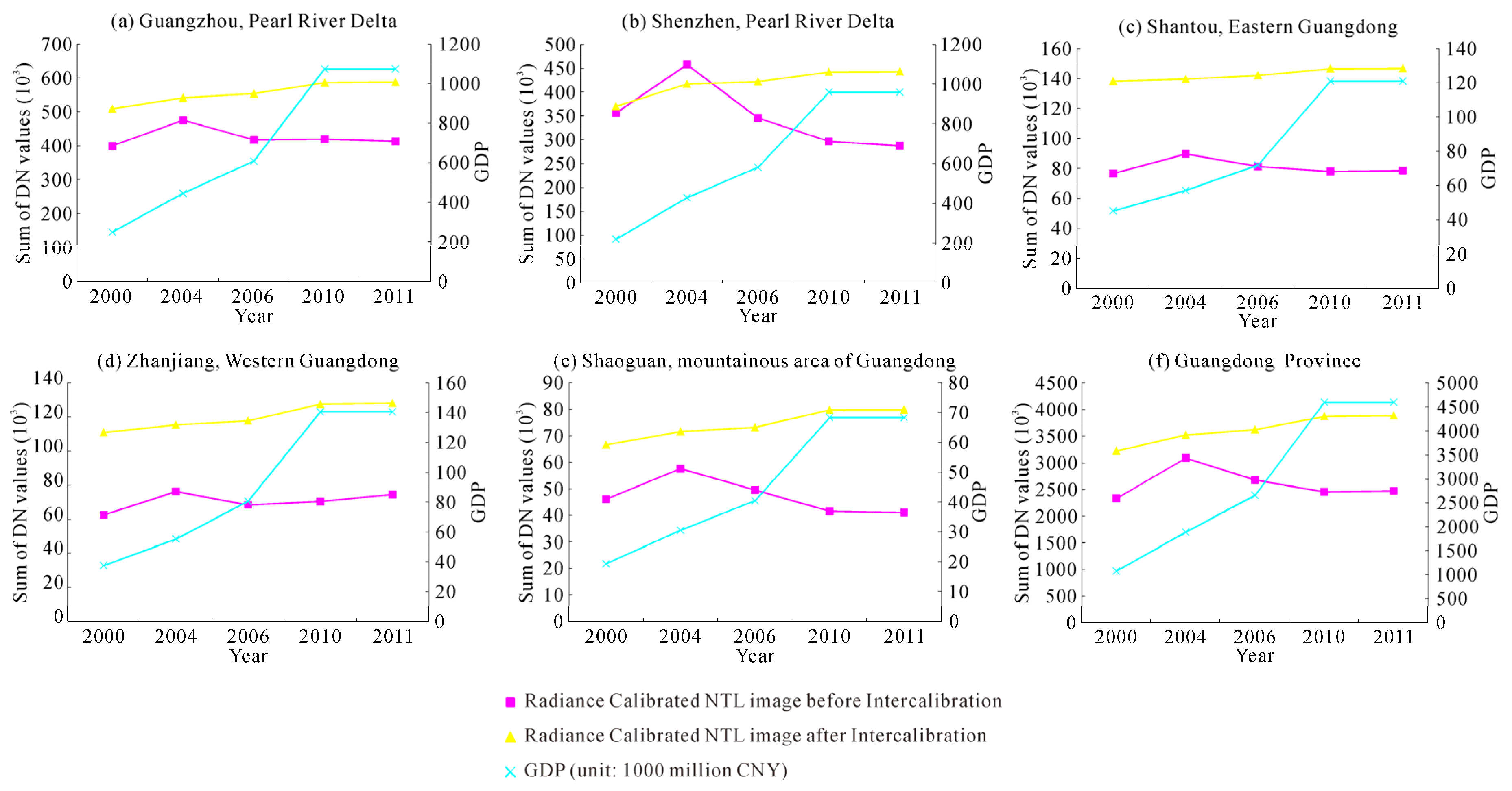
4.1. Verifying the Intercalibration Results of Radiance-Calibrated Time Series Images

In order to verify the results of the intercalibration of RC NTL time series images for Guangdong, the sum of light intensity (DN values) are compared between the RC NTL and IC-RC NTL images. To ensure the reliability of this comparison, five cities in different regions of Guangdong distributed throughout the province were selected as the areas for the comparison. The five cities are Guangzhou and Shenzhen in the Pearl River delta, Shantou in the eastern area of Guangdong, Zhanjiang in the western area of Guangdong and Shaoguan in the mountainous area of Guangdong. Guangzhou and Shenzhen are taken to represent the Pearl River delta, and the other three cities are representative of their corresponding regions. Therefore, the five cities can represent the four regions of Guangdong. In addition, GDP statistical data is used as ancillary data to facilitate this comparison (Figure 5).
Figure 5. The comparison among the RC NTL images, the IC-RC NTL images and GDP statistical data. (a) Guangzhou and (b) Shenzhen in the Pearl River delta; (c) Shantou in eastern area of Guangdong; (d) Zhanjiang in western area of Guangdong; (e) Shaoguan in the mountainous area of Guangdong and (f) Guangdong province overall.
Sustainability 08 00108 g005
In Figure 5, the variation in the sum of DN values of IC-RC NTL images are all generally suppressed among the various years. The sum of DN values in the 2004 RC NTL image is larger than the reference year of 2006, and the sum of DN values in the 2010 and 2010_2011 RC NTL images are less than the reference year of 2006. Therefore, before intercalibration, the 2004 RC NTL image was overestimated, while the 2010 and 2010_2011 images were underestimated. Additionally, before intercalibration, the trend of overall sum of DN values of RC NTL images was unstable at both the municipal and provincial levels. However, after intercalibration, the sum of DN values appears to gradually increase. This trend is the same for the overall GDP change in these cities and for the entire Guangdong Province. Although the intercalibrated images show a generally increasing trend, the increase in GDP is much steeper. This illustrates that the speed of economic growth is significantly greater than the rate of the human activity intensification. The fact that the DN values do not show such rapid increases illustrate that the overestimate in 2004 and the underestimates in 2010 and 2010_2011 have not been eliminated even though these images had been corrected. In conclusion, this intercalibration method has a certain rationality and the result could be acceptable.
To further test the results of the intercalibration, a comparison between RC NTL images and IC-RC NTL images was conducted. Guangzhou and Shenzhen were selected for this comparison. The pixels whose DN value were equal to 63 (saturation value) in the F182010 NSL image were assumed as the urban core. The urban core was then used as mask to extract the corresponding area of the RC NTL images and IC-RC NTL images for 2000, 2004, 2006, 2010 and 2010_2011. Finally, the sum of DN values in the urban core are compared for these two types of RC NTL images. The results are shown in Table 3.
Table 3. Comparison of DN sums between the RC NTL images and IC-RC NTL images in Guangzhou and Shenzhen.
CityYearRC NTL ImagesIC-RC NTL Images
Urban CoreWhole UrbanUrban CoreWhole Urban
Guangzhou2000117,364 399,590103,177508,855
2004112,311 474,931108,411541,923
200691,204 417,618110,632553,827
201097,775 419,465111,817586,157
2010_2011100,170 413,052111,824588,204
Shenzhen2000152,806 355,733126,256369,792
2004183,370 457,437149,434416,756
2006115,359 345,483149,452421,767
201087,445 296,498150,087441,978
2010_201184,579 287,314150,087442,839
In Table 3, both in Guangzhou and Shenzhen, the sum of DN values of RC NTL images are fluctuant and the overall trend is decreasing. This trend and fast economic growth is contradictory. Therefore, this illustrates that DN sums for 2000 and 2004 RC NTL images before the reference year of 2006 have been overestimated, while the values for 2010 and 2010_2011 have been underestimated. After intercalibration, the overall trend for the sum of DN values gradually grows in both the urban core and for the whole city. This trend is the same with the development situation for the last twenty years in Guangzhou, Shenzhen and Guangdong province. This result illustrates that the intercalibration method proposed in this study improved the RC NTL images and that this method is rational and feasible.
Additionally, linear regression analysis was applied in this study and the coefficients between GDP23 and RC NTL images as well as intercalibrated RC NTL images (IC-RC NTL images) and RC NTL images subjected to both intercalibration and light overflow correction (T-IC-RC NTL images) are compared at the county level (Table 4). In Table 4, the linear correlation coefficients between GDP23 and RC NTL images are larger than those of intercalibrated RC NTL images in 2000 and 2010. However, the coefficients of RC NTL images are less than IC-RC NTL images in 2004 and 2006. Since all RC NTL images are intercalibrated via the 2006 RC NTL image and the time interval between 2000 and 2006 and between 2006 and 2010 are excessively long, the pixel value of the 2000 and 2010 RC NTL images are corrected to be closer to the 2006 RC NTL image. Therefore, these images have a weaker relationship with GDP23 after intercalibration. In contrast, the relationship between RC NTL images and GDP23 becomes stronger in 2004 and 2006.
Table 4. The comparison of linear correlation coefficients.
YearRC NTL ImageIC-RC NTL Image *T-IC-RC NTL Image *
20000.83730.80020.7988
20040.77540.79490.7957
20060.83830.85180.8541
20100.88620.86120.8623
* IC-RC NTL image is the intercalibrated RC NTL image, while T-IC-RC NTL image is RC NTL image that is subjected to both intercalibration and light overflow correction.
Despite the correlation coefficient decline after the calibration in 2000 and 2010, the intercalibration is also necessary because the 2000 and 2010 RC NTL images and the estimated GDP density maps based on these two images cannot compare without intercalibration. However, these images are comparable after intercalibration because all RC NTL images have the same reference image. After intercalibration, the temporal change of light intensity exhibits greater correspondence with the economic development status of Guangdong. Therefore, the results of the intercalibration are acceptable and relatively plausible.

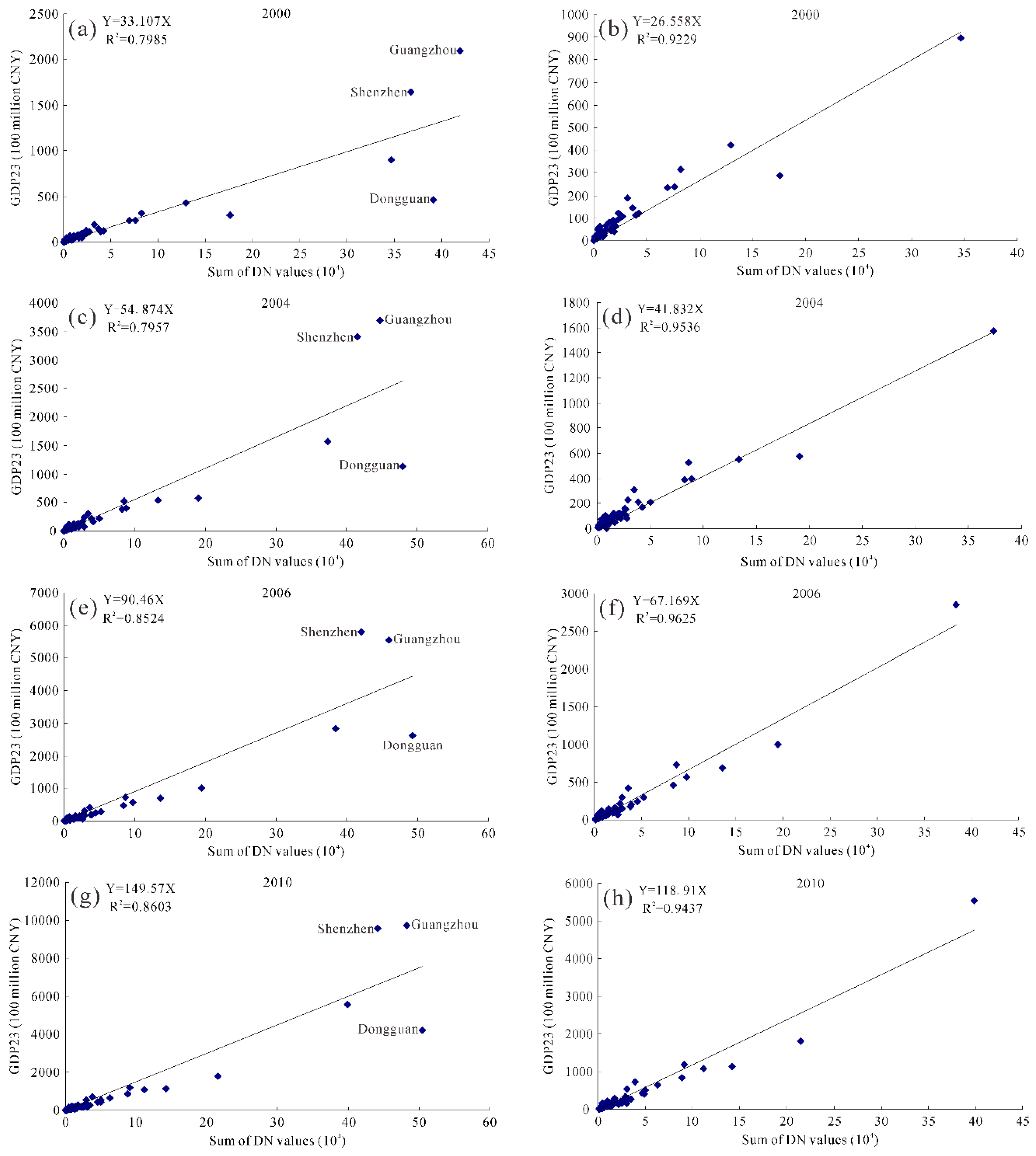
4.2. Accuracy Assessment Results for the Estimated GDP in Guangdong Province

The relative error (Equation (8)) between statistical data and estimated data is used to assess the accuracy of the estimated secondary and tertiary industry production (GDP23). Then, a direct comparison of the absolute value of relative error (|RE|) is conducted at the county-level for Guangdong province to assess the accuracy of GDP23 estimated from the RC NTL images. This comparison was done for both the RC NTL images that were subjected to intercalibration and light overflow correction (T-IC-RC NTL images) (Figure 4a,c,e,g), and RC NTL images that were subjected to intercalibration, light overflow correction, and outlier removal (RO-T-IC-RC NTL images) (Figure 4b,d,f,h).
R E = ( G D P e G D P s ) / G D P s
RE is the relative error, GDPs is the GDP statistical data, and GDPe is the estimated GDP.
The methods for estimating GDP23 (Figure 4) used the county-level administrative unit as the basic unit of this study, and the RE is also calculated at the county level. A city-level RE is also calculated. The accuracy comparison of GDP23 spatialization based on different types of NTL data is carried out at these levels.
In order to facilitate comparison, absolute relative error values (|RE|) are divided into four levels: |RE| ≤ 0.35 is regarded as level 1; |RE| in the range of 0.35 to 0.7 is regarded as level 2; |RE| in the range of 0.7 to 1.0 is regarded as level 3; and |RE| ≥ 1.0 is regarded as level 4.
Table 5 shows the number of each level of |RE| between estimated GDP based on different types of RC NTL images and GDP statistical data at the county and city level, respectively. |RE| is the absolute relative error values between GDP23 statistical data and estimated GDP23 based on three different types of RC NTL images. At the county level, the number of level 1 |RE| for estimated GDP23 based on RO-T-IC-RC NTL images is higher than the other image types for 2004, 2006 and 2010. The number of level 2 |RE| for estimated GDP23 based on RO-T-IC-RC NTL images is the highest. Therefore, when |RE| ≤ 0.35 or |RE| ≤ 0.7, there are a relatively greater number of samples for estimated GDP23 based on RO-T-IC-RC NTL images. The accuracy of estimated GDP23 based on this type of RC NTL images is at best a speculation. At city level in 2000 and 2004, the number of level 1 |RE| for estimated GDP23 based on RO-T-IC-RC NTL images is slightly less than for RC NTL images. However, RO-T-IC-RC NTL exhibits the highest number of level 1 |RE| in other years and the highest number of level 2 |RE| in all four years. Therefore, the accuracy of estimated GDP23 based on RO-T-IC-RC NTL images can be supposed to be the best at the city level. Hence, the highest accuracy of estimated GDP23 was derived from RC NTL images subjected to intercalibration, light overflow corrected, and outlier removal (RO-T-IC-RC NTL) images.
Table 5. The number of each level of absolute relative error values between estimated GDP23 based on different types of RC NTL images and GDP statistical data at the county and city level.
NTL ImageLevel2000200420062010
CountyCityCountyCityCountyCityCountyCity
RC NTL image138144014127145
2285214204124
360611762110
4102152334352
T-IC-RC NTL image *12913218105135
22021978090
3112134126128
42242925210488
RO-T-IC-RC NTL image *13210441352194714
24210347292297
370410040
411001020
* T-IC-RC NTL images are the RC NTL images that were subjected to intercalibration and light overflow correction; RO-T-IC-RC NTL image are RC NTL images that were subjected to intercalibration, light overflow correction, and outlier removal.

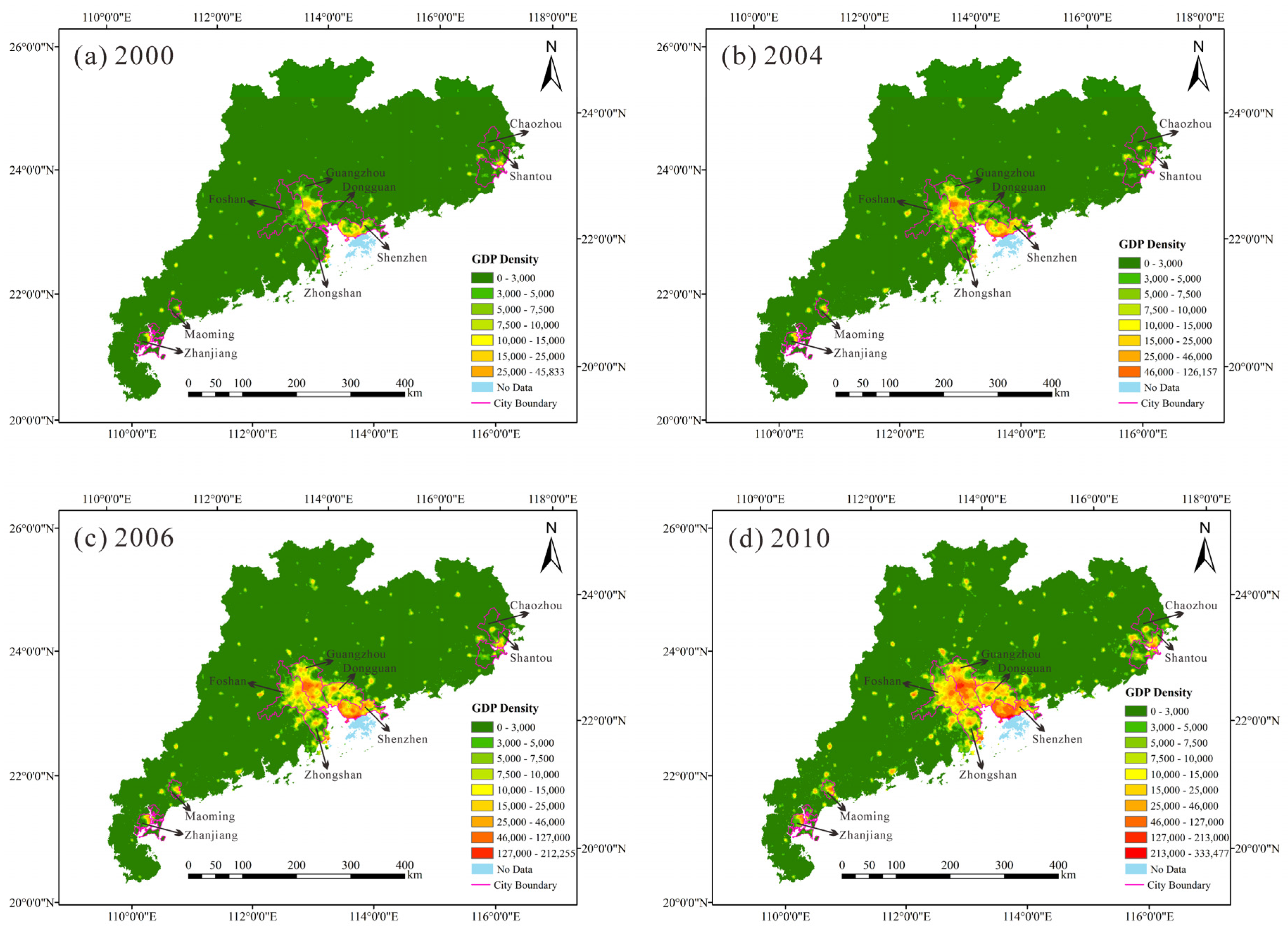
4.3. Comparison and Analysis of GDP Density of Guangdong Province in 2000, 2004, 2006 and 2010

Figure 6 depicts four 1 km gridded GDP density images of Guangdong province for 2000, 2004, 2006 and 2010. The secondary and tertiary industry production were estimated by using the correlation between RO-T-IC-RC NTL images and county-level GDP statistic data. The primary industry production was calculated based on the land use/cover data.
Figure 6. GDP density map of Guangdong Province. (unit: 10 million CNY/1 km2). (a) 2000; (b) 2004; (c) 2006; (d) 2010.
Sustainability 08 00108 g006
In Figure 6, most of the high GDP density areas are concentrated in the Pearl River delta and the Chaoshan areas in eastern Guangdong. These two areas are both plain regions (the Pearl River delta plain and Chaoshan plain) and have high levels of urbanization. In addition, some coastal areas exhibit high GDP density values. At the county level, the city-governed districts of Guangzhou and Shenzhen have the highest GDP density. The counties of the Pearl River delta have the highest overall values in terms of GDP density and with respect to the areal extent of the high GDP density regions. Some counties in western Guangdong (e.g., Zhanjiang and Maoming) and eastern Guangdong (e.g., Shantou and Chaozhou) also present relatively high GDP density values. Compared with these three regions, the GDP density of counties in the northern mountainous area of Guangdong is the lowest. The GDP density in Guangdong province is distributed, in descending order, in the Pearl River delta, eastern and western Guangdong, and the northern mountainous area of Guangdong.
By comparing images (a), (b), (c), and (d) of Figure 6, the changes in the GDP density of Guangdong province can be analyzed. At the provincial level, the area of relatively high (we define GDP density values > 70 million/km2 as relatively high in this study) GDP density is rapidly increasing. At the county level, the GDP density of counties in the Pearl River delta, especially the city-governed districts of Foshan, Dongguan, and Zhongshan, rapidly increased during 2000 and 2010. During the same period, the areas of relatively high GDP density in the Pearl River delta generally expanded. Although some counties in eastern Guangdong and western Guangdong exhibited increases in GDP density, the areas of relatively high GDP density remained nearly unchanged. The counties in the northern mountainous area of Guangdong exhibited the smallest changes in GDP density. These results indicate that, on average, the Pearl River delta developed from 2000 to 2010. The rapid development of Guangzhou and Shenzhen spurred the economic development of Foshan, Dongguan, Zhongshan and other surrounding cities. In turn, the rapid development of these neighboring cities could also promote more rapid development in Guangzhou and Shenzhen. This interaction mechanism created more rapid and substantial development of the regional economy in the Pearl River delta. Unlike the Pearl River delta area, the counties of eastern Guangdong, western Guangdong and the northern mountainous area of Guangdong often develop independently, and the rapid development of a certain county does not spur the economic development of the surrounding ones. This may be one reason for the slower economic development in these areas compared to counties in the Pearl River delta area.

5. Conclusions

The NTL images facilitate the effective estimation of GDP at different spatial scales, but the problems of pixel saturation and light overflow in these datasets limit the accuracy of such estimations. Therefore, DMSP/OLS radiance-calibrated nighttime light (RC NTL) images which did not include saturated pixels were utilized in this study to estimate GDP spatialization at the sub-national scale. On the basis of previous studies, this paper presented an intercalibration method for DMSP/OLS RC NTL time series images of Guangdong based on the invariant region method. This approach solved the comparability problem in the RC NTL dataset. We implemented this method to obtain intercalibrated RC NTL images for Guangdong and tested the intercalibrated results. These test results support the effectiveness of this intercalibration method and suggest that the intercalibrated results are acceptable.
We derived four 1 km gridded GDP density images of Guangdong province for 2000, 2004, 2006, and 2010 by using corrected RC NTL data and land use/cover data. To improve the accuracy of the estimated results, the threshold value method based on MODIS NDVI images was developed to reduce the light overflow effect. The estimation of secondary and tertiary industry production was based on the correlation between both the intercalibrated and light overflow corrected RC NTL images after removing outliers (RO-T-IC-RC NTL images) and the GDP23 statistical data at the county level of Guangdong. The estimation of primary industry production was based on land use/cover data. We compared and analyzed the GDP density images of the above four years and summarized the economic development trend of Guangdong province. In terms of both the total GDP value and GDP growth, the counties of the Pearl River delta area have the highest values. The counties in the northern mountainous area of Guangdong have the lowest values, and the counties of eastern Guangdong and western Guangdong have intermediate values.
The GDP density map offers a straightforward and visible means of studying the spatial heterogeneity of economic development. The images can serve not only as crucial reference data for the government and various organizations when formulating development strategies and policies, but it can also be useful in exposure and risk analysis.

Acknowledgments

This study was supported by the National Natural Science Foundation of China (41171446). The authors would like to thank the editor and the anonymous reviewers for their helpful comments and suggestions.

Author Contributions

Ziyang Cao and Zhifeng Wu conceived and designed this study. Ziyang Cao made substantial contributions to acquisition, analysis, and interpretation of the data. Zhifeng Wu made important contributions to conception and structure of this article. Ziyang Cao wrote the first draft of the article. Zhifeng Wu, Yaoqiu Kuang and Ningsheng Huang reviewed and edited the first draft. All authors read and approved the submitted manuscript, agreed to be listed, and accepted the version for publication.

Conflicts of Interest

The authors declare no conflict of interest.

References

  1. Stevenson, R.J.; Sabater, S. Understanding effects of global change on river ecosystems: Science to support policy in a changing world. Hydrobiologia 2010, 657, 3–18. [Google Scholar] [CrossRef]
  2. Sang, X.F.; Zhou, Z.H.; Wang, H.; Qin, D.Y.; Zhai, Z.L.; Chen, Q. Development of soil and water assessment tool model on human water use and application in the area of high human activities, Tianjin, China. J. Irrig. Drain. Eng. 2010, 136, 23–30. [Google Scholar] [CrossRef]
  3. Huo, Z.L.; Feng, S.Y.; Kang, S.Z.; Dai, X.Q.; Li, W.C.; Chen, S.J. The response of water-land environment to human activities in arid minqin oasis, northwest china. Arid Land Res. Manag. 2007, 21, 21–36. [Google Scholar] [CrossRef]
  4. Wang, J.N.; Lu, Y.T.; Zhou, J.S.; Li, Y.; Cao, D. Analysis of China resource-environment Gini coefficient based on GDP. China Environ. Sci. 2006, 26, 111–115. [Google Scholar]
  5. Chen, K.P.; McAneney, J.; Blong, R.; Leigh, R.; Hunter, L.; Magill, C. Defining area at risk and its effect in catastrophe loss estimation: A dasymetric mapping approach. Appl. Geogr. 2004, 24, 97–117. [Google Scholar] [CrossRef]
  6. Thieken, A.H.; Muller, M.; Kleist, L.; Seifert, I.; Borst, D.; Werner, U. Regionalisation of asset values for risk analyses. Nat. Hazards Earth Syst. Sci. 2006, 6, 167–178. [Google Scholar] [CrossRef]
  7. Liu, H.H.; Jiang, D.; Yang, X.H.; Luo, C. Spatialization Approach to 1 km Grid GDP Supported by Remote Sensing. Geoinf. Sci. 2005, 7, 120–123. [Google Scholar]
  8. Han, X.D.; Zhou, Y.; Wang, S.X.; Liu, R.; Yao, Y. GDP spatializarion in China based on nighttime imagery. J. Geoinf. Sci. 2012, 14, 128–136. [Google Scholar]
  9. Elvidge, C.; Baugh, K.; Hobson, V.; Kihn, E.; Kroehl, H.; Davis, E.; Cocero, D. Satellite inventory of human settlements using nocturnal radiation emissions: A contribution for the global toolchest. Glob. Chang. Biol. 1997, 3, 387–395. [Google Scholar] [CrossRef]
  10. Elvidge, C.D.; Baugh, K.E.; Dietz, J.B.; Bland, T.; Sutton, P.C.; Kroehl, H.W. Radiance calibration of DMSP-OLS low-light imaging data of human settlements. Remote Sens. Environ. 1999, 68, 77–88. [Google Scholar] [CrossRef]
  11. Elvidge, C.D.; Imhoff, M.L.; Baugh, K.E.; Hobson, V.R.; Nelson, I.; Safran, J.; Dietz, J.B.; Tuttle, B.T. Night-time lights of the world: 1994–1995. ISPRS J. Photogramm. Remote Sens. 2001, 56, 81–99. [Google Scholar] [CrossRef]
  12. Doll, C.N.H.; Muller, J.-P.; Morley, J.G. Mapping regional economic activity from night-time light satellite imagery. Ecol. Econ. 2006, 57, 75–92. [Google Scholar] [CrossRef]
  13. Elvidge, C.D.; Sutton, P.C.; Ghosh, T.; Tuttle, B.T.; Baugh, K.E.; Bhaduri, B.; Bright, E. A global poverty map derived from satellite data. Comput. Geosci. 2009, 35, 1652–1660. [Google Scholar] [CrossRef]
  14. Elvidge, C.D.; Baugh, K.E.; Kihn, E.A.; Kroehl, H.W.; Davis, E.R.; Davis, C.W. Relation between satellite observed visible-near infrared emissions, population, economic activity and electric power consumption. Int. J. Remote Sens. 1997, 18, 1373–1379. [Google Scholar] [CrossRef]
  15. Doll, C.H.; Muller, J.-P.; Elvidge, C.D. Night-time imagery as a tool for global mapping of socioeconomic parameters and greenhouse gas emissions. Ambio 2000, 29, 157–162. [Google Scholar] [CrossRef]
  16. Wang, Q.; Yuan, T.; Zheng, X.Q. GDP gross analysis at province-level in China based on night-time lightsatellite imagery. Urban Dev. Stud. 2013, 20, 44–48. [Google Scholar]
  17. Cao, X.; Wang, J.; Chen, J.; Shi, F. Spatialization of electricity consumption of china using saturation-corrected DMSP-OLS data. Int. J. Appl. Earth Obs. Geoinf. 2014, 28, 193–200. [Google Scholar] [CrossRef]
  18. Wang, W.; Cheng, H.; Zhang, L. Poverty assessment using DMSP/OLS night-time light satellite imagery at a provincial scale in China. Adv. Space Res. 2012, 49, 1253–1264. [Google Scholar] [CrossRef]
  19. Takahashi, K.I.; Terakado, R.; Nakamura, J.; Adachi, Y.; Elvidge, C.D.; Matsuno, Y. In-use stock analysis using satellite nighttime light observation data. Resour. Conserv. Recycl. 2010, 55, 196–200. [Google Scholar] [CrossRef]
  20. Liang, H.W.; Tanikawa, H.; Matsuno, Y.; Dong, L. Modeling in-use steel stock in china’s buildings and civil engineering infrastructure using time-series of DMSP/OLS nighttime lights. Remote Sens. 2014, 6, 4780–4800. [Google Scholar] [CrossRef]
  21. Zhang, L.; Qu, G.; Wang, W. Estimating land development time lags in China using DMSP/OLS nighttime light image. Remote Sens. 2015, 7, 882–904. [Google Scholar] [CrossRef]
  22. Sutton, P.C.; Costanza, R. Global estimates of market and non-market values derived from nighttime satellite imagery, land cover, and ecosystem service valuation. Ecol. Econ. 2002, 41, 509–527. [Google Scholar] [CrossRef]
  23. Ghosh, T.; Powell, R.L.; Elvidge, C.D.; Baugh, K.E.; Sutton, P.C.; Anderson, S. Shedding light on the global distribution of economic activity. Open Geogr. J. 2010, 3, 148–161. [Google Scholar]
  24. Han, X.D.; Zhou, Y.; Wang, S.X.; Liu, R.; Yao, Y. GDP spatialization in China based on DMSP/OLS data and land use data. Remote Sens. Technol. Appl. 2012, 27, 396–405. [Google Scholar]
  25. Yang, Y.; Wu, L.L.; Deng, S.L.; Zhang, C. Spatialization method of provincial statistical GDP data based on DMSP/OLS night lighting data: A case study of Guangxi Zhuang Autonomous Region. Geogr. Geoinf. Sci. 2014, 30, 108–111. [Google Scholar]
  26. Elvidge, C.D.; Cinzano, P.; Pettit, D.R.; Arvesen, J.; Sutton, P.; Small, C.; Nemani, R.; Longcore, T.; Rich, C.; Safran, J.; et al. The nightsat mission concept. Int. J. Remote Sens. 2007, 28, 2645–2670. [Google Scholar] [CrossRef]
  27. Imhoff, M.L.; Lawrence, W.T.; Stutzer, D.C.; Elvidge, C.D. A technique for using composite DMSP/OLS “city lights” satellite data to map urban area. Remote Sens. Environ. 1997, 61, 361–370. [Google Scholar] [CrossRef]
  28. Letu, H.; Bao, Y.H.; Tana, G.; Hara, M.; Nishio, F. Relationship between DMSP/OLS nighttime light and CO2 emission from electric power plant. Land Surf. Remote Sens. 2012. [Google Scholar] [CrossRef]
  29. Zhang, Q.; Schaaf, C.; Seto, K.C. The vegetation adjusted ntl urban index: A new approach to reduce saturation and increase variation in nighttime luminosity. Remote Sens. Environ. 2013, 129, 32–41. [Google Scholar] [CrossRef]
  30. Small, C.; Elvidge, C.D.; Balk, D.; Montgomery, M. Spatial scaling of stable night lights. Remote Sens. Environ. 2011, 115, 269–280. [Google Scholar] [CrossRef]
  31. Yue, W.Z.; Gao, J.B.; Yang, X.C. Estimation of gross domestic product using multi-sensor remote sensing data: A case study in Zhejiang province, East China. Remote Sens. 2014, 6, 7260–7275. [Google Scholar] [CrossRef]
  32. Ziskin, D.; Baugh, K.; Hsu, F.-C.; Elvidge, C.D. Methods used for the 2006 radiance lights. Proc. Asia Pac. Adv. Netw. 2010, 30, 131–142. [Google Scholar] [CrossRef]
  33. Hsu, F.-C.; Baugh, K.E.; Ghosh, T.; Zhizhin, M.; Elvidge, C.D. Dmsp-ols radiance calibrated nighttime lights time series with intercalibration. Remote Sens. 2015, 7, 1855–1876. [Google Scholar] [CrossRef]
  34. Lu, D.; Tian, H.; Zhou, G.; Ge, H. Regional mapping of human settlements in Southeastern China with multisensor remotely sensed data. Remote Sens. Environ. 2008, 112, 3668–3679. [Google Scholar] [CrossRef]
  35. Zhuo, L.; Zheng, J.; Zhang, X.; Li, J.; Liu, L. An improved method of night-time light saturation reduction based on EVI. Int. J. Remote Sens. 2015, 36, 4114–4130. [Google Scholar] [CrossRef]
  36. National Bureau of Statistics of China. China Statistical Yearbook 2010; China Statistics Press: Beijing, China, 2010. Available online: http://www.stats.gov.cn/tjsj/ndsj/ (accessed on 15 October 2015). (In Chinese)
  37. National Oceanic and Atmospheric Administration (NOAA)/National Geography Data Center (NGDC) Website. Available online: http://ngdc.noaa.gov/eog/download.html (accessed on 24 September 2015).
  38. National Aeronautics and Space Administration (NASA)/Goddard Space Flight Center (GSFC) Website. Available online: http://ladsweb.nascom.nasa.gov/data/search.html (accessed 7 October 2015).
  39. Fensholt, R.; Rasmussen, K.; Nielsen, T.T.; Mbow, C. Evaluation of earth observation based long term vegetation trends–intercomparing ndvi time series trend analysis consistency of sahel from avhrr gimms, terra modis and spot vgt data. Remote Sens. Environ. 2009, 113, 1886–1898. [Google Scholar] [CrossRef]
  40. Tarnavsky, E.; Garrigues, S.; Brown, M.E. Multiscale geostatistical analysis of avhrr, spot-vgt, and modis global ndvi products. Remote Sens. Environ. 2008, 112, 535–549. [Google Scholar] [CrossRef]
  41. Huete, A.; Didan, K.; Miura, T.; Rodriguez, E.P.; Gao, X.; Ferreira, L.G. Overview of the radiometric and biophysical performance of the modis vegetation indices. Remote Sens. Environ. 2002, 83, 195–213. [Google Scholar] [CrossRef]
  42. Resources and Environment Data Center of the Chinese Academy of Science Website. Available online: http://www.resdc.cn (accessed on 10 October 2015).
  43. Liu, J.; Liu, M.; Zhuang, D.; Zhang, Z.; Deng, X. Study on spatial pattern of land-use change in China during 1995–2000. Sci. China Ser. D Earth Sci. 2003, 46, 373–384. [Google Scholar]
  44. Ebener, S.; Murray, C.; Tandon, A.; Elvidge, C. From wealth to health: Modelling the distribution of income per capita at the sub-national level using night-time light imagery. Int. J. Health Geogr. 2005. [Google Scholar] [CrossRef] [PubMed]
  45. Liu, J.Y.; Zhang, Z.X.; Xu, X.L.; Kuang, W.H.; Zhou, W.C.; Zhang, S.W.; Li, R.D.; Yan, C.Z.; Yu, D.S.; Wu, S.X.; et al. Spatial patterns and driving forces of land use change in China during the early 21st century. J. Geogr. Sci. 2010, 20, 483–494. [Google Scholar] [CrossRef]
  46. Statistics Bureau of Guangdong Province. Guangdong Statistical Yearbook; China Statistics Press: Beijing, China, 2001, 2005, 2007, 2011. Available online: http://www.gdstats.gov.cn/tjsj/gdtjnj/ (accessed on 15 October 2015). (In Chinese)
  47. Statistics Bureau of Guangdong Province. Agricultural Statistical Yearbook of Guangdong; China Statistics Press: Beijing, China, 2011. Available online: http://www.gdstats.gov.cn/tjsj/gdtjnj/ (accessed on 15 October 2015). (In Chinese)
  48. Hall, F.G.; Strebel, D.E.; Nickeson, J.E.; Goetz, S.J. Radiometric rectification—toward a common radiometric response among multidate, multisensor images. Remote Sens. Environ. 1991, 35, 11–27. [Google Scholar] [CrossRef]
  49. Coppin, P.R.; Bauer, M.E. Processing of multitemporal Landsat TM imagery to optimize extraction of forest cover change features. IEEE Trans. Geosci. Remote Sens. 1994, 32, 918–927. [Google Scholar] [CrossRef]
  50. Lenney, M.P.; Woodcock, C.E.; Collins, J.B.; Hamdi, H. The status of agricultural lands in Egypt: The use of multitemporal ndvi features derived from Landsat TM. Remote Sens. Environ. 1996, 56, 8–20. [Google Scholar] [CrossRef]
  51. Elvidge, C.; Ziskin, D.; Baugh, K.; Tuttle, B.; Ghosh, T.; Pack, D.; Erwin, E.; Zhizhin, M. A fifteen year record of global natural gas flaring derived from satellite data. Energies 2009, 2, 595–622. [Google Scholar] [CrossRef]
  52. Liu, Z.; He, C.; Zhang, Q.; Huang, Q.; Yang, Y. Extracting the dynamics of urban expansion in China using DMSP-OLS nighttime light data from 1992 to 2008. Landsc. Urban Plan. 2012, 106, 62–72. [Google Scholar] [CrossRef]
  53. Zhao, N.; Currit, N.; Samson, E. Net primary production and gross domestic product in China derived from satellite imagery. Ecol. Econ. 2011, 70, 921–928. [Google Scholar] [CrossRef]

