Delineating Urban Boundaries Using Landsat 8 Multispectral Data and VIIRS Nighttime Light Data
by
 , ,
, ,
Xingyu Xue
 ,
,
Zhoulu Yu
,
Shaochun Zhu
,
Qiming Zheng
,
Melanie Weston
,
Ke Wang
*,
Muye Gan
and
Hongwei Xu
Institute of Applied Remote Sensing and Information Technology, College of Environmental and Resource Sciences, Zhejiang University, Hangzhou 310058, China
*
Author to whom correspondence should be addressed.
Remote Sens. 2018, 10(5), 799; https://doi.org/10.3390/rs10050799
Submission received: 5 March 2018
/
Revised: 11 May 2018
/
Accepted: 17 May 2018
/
Published: 21 May 2018
(This article belongs to the Special Issue Remote Sensing of Night Lights – Beyond DMSP)
Abstract
:Administering an urban boundary (UB) is increasingly important for curbing disorderly urban land expansion. The traditionally manual digitalization is time-consuming, and it is difficult to connect UB in the urban fringe due to the fragmented urban pattern in daytime data. Nighttime light (NTL) data is a powerful tool used to map the urban extent, but both the blooming effect and the coarse spatial resolution make the urban product unable to meet the requirements of high-precision urban study. In this study, precise UB is extracted by a practical and effective method using NTL data and Landsat 8 data. Hangzhou, a megacity experiencing rapid urban sprawl, was selected to test the proposed method. Firstly, the rough UB was identified by the search mode of the concentric zones model (CZM) and the variance-based approach. Secondly, a buffer area was constructed to encompass the precise UB that is near the rough UB within a certain distance. Finally, the edge detection method was adopted to obtain the precise UB with a spatial resolution of 30 m. The experimental results show that a good performance was achieved and that it solved the largest disadvantage of the NTL data-blooming effect. The findings indicated that cities with a similar level of socio-economic status can be processed together when applied to larger-scale applications.
1. Introduction
In the background of global urbanization, urbanization impacts on the natural ecosystems and social systems are increasingly concerning [1,2,3]. The urbanization rate in China almost doubled to 56.1% in 2015 compared to that of 1980. It is vital to distinguish these urban boundaries (UBs), especially in developing countries [4]. China’s Ministry of Land and Resource pointed out that there is an urgent need to identify urban boundaries (UBs) in megacities, such as Beijing, Shanghai, Guangzhou, and Hangzhou. UBs are lines that encompass the urban land cover in a limited extent, which include urban green space, urban impervious surfaces, urban waters, and so on. Once these UB(s) have been delineated, the new built-up land will be limited inside the UB. All in all, UB is a very important concept in urban planning, especially in developing countries. In addition to the applications in urban planning, it is also important that scientific research needs to delimit urban areas, such as the different protection goals for urban and rural ecosystem services [5]. However, few studies have aimed at delineating UB.
In urban planning, UBs are usually derived from manual digitalization from remote sensing (RS) imagery. It is troublesome work and cannot meet the requirements of large-scale future urban planning work. The classification in RS is the most common method to extract urban areas [6,7,8], but classification accuracy often suffers from the classification algorithms and the design of class schemes [9]. Furthermore, the process is time-consuming. Hence, spectral indices, such as the normalized difference impervious surface index (NDISI) are popular due to their easy implementation [10,11]. However, a limitation is user bias, as the threshold slicing between the urban and non-urban area is determined by personal judgment and the Government Finance Statistics Yearbook [12]. Unlike the extraction of urban impervious surfaces in RS, continuity is a basic requirement of UB. These indices and classification methods can result in fragmented classification results which were intricately covered with urban green space, urban waters, and urban impervious surfaces. This phenomenon will bring some difficulties when connecting the UB.
Nighttime light (NTL) data is spatially continuous over large areas which compensates for the above disadvantages to some extent. NTL data has shown a positive correlation with human activities, such as the gross domestic product (GDP) and the built-up area at the significant level [13,14,15,16,17]. Numerous studies have highlighted that NTL provides a reliable source to map the regional and global urban extent [18], utilizing methods, such as SVM-based classification [19], one-class classification, and thresholding [20,21]. The thresholding method, including both the global-fixed and locally optimized thresholding [22,23,24], is often used to extract urban areas because of its simplicity. Previous studies demonstrated that the appropriate thresholds vary with regions depending on their different socio-economic states [25]. This means that the uniform regional and global thresholds would result in the overestimation of large cities because of the blooming effect of NTL and the underestimation of small cities [26]. The blooming effect is a phenomenon in NTL imagery where urban peripheries are brightened by urban lights. Lit areas in original NTL imagery are larger than actual urban areas [27]. Furthermore, the coarse spatial resolution of NTL data itself will affect the accuracy of urban extent. Owing to these limitations, most NTL urban studies have been limited to large scales, such as continental and global scales. Hence, there is an urgent demand for a product with improved spatial resolution and accuracy for future urban planning [28].
Multiple research studies have attempted to improve the accuracy of extracting the spatial extent of urban areas. For example, an inside buffer method was applied to resolve the overestimation [26]. A large number of indices, such as the vegetation adjusted NTL urban index (VANUI), were proposed to reduce the saturation effect and successfully enhance the inner-urban variation of DMSP/OLS NTL data [29]. The neighborhood statistics analysis (NSA) method has divided the region into transition zones, urban, and rural areas for the precise extraction of the urban extent [30]. A cluster-based method was developed to estimate the optimal threshold and to map the urban extent [25]. All in all, the methods applied in NTL urban studies are either complicated or inaccurate. Seldom studies have reached a balance between complexity and accuracy. An effective and relatively high-accuracy method has great practicability and will expand the application scope of NTL data. Among these technologies, the primary method to identify urban areas is the threshold method because of its simplicity. In reality, even in a single megacity, both overestimation and underestimation exist, although the total urban area is exaggerated. However, research has seldom focused on this phenomenon.
Among these proposed methods, VANUI is a compound index which consists of the normalized difference vegetation index (NDVI) and NTL data. Previous studies have demonstrated that the detailed information of land cover in the urban fringe was extensively enhanced by this index [31]. Thus, the demarcation line between urban and rural area becomes more distinguished. Therefore, it allows for the feasible precise extraction of UB.
In this paper, we propose to develop a novel and multiple-step approach which accurately identifies the UB by combining Landsat 8 OLI (Operational Land Imager) with NTL data. It is based on the hypotheses that there is an urban fringe where spatial patterns of land cover are the most complex and the NTL intensity is low. Hence, in the urban fringe the demarcation line among different types of land cover is the UB. The following objectives were undertaken: (1) rough UB, which has relatively lower accuracy compared with precise UB, was located through the variance index and the search mode of the concentric zone model (CZM); (2) an inside and outside buffer was established to encompass the precise UB; and (3) delineation of the precise UB utilizing the revised Canny edge detection algorithm in the urban fringe [32,33,34]. The UB extraction method will be verified by accuracy assessments and comparative analyses. The suitability of the mechanism and the universality of our proposed method will be elaborated in the discussion section. In the final section, conclusions and future works are provided.
2. The Study Area and Background Knowledge
2.1. Definition of Urban, Rural Area, and Urban Boundary
UB is considered as the demarcation line between urban and rural areas. However, a general definition of UB is absent since the term urban and rural have different definitions in different fields [35,36]. In this work, we defined urban and rural from the perspective of RS. According to previous studies, the scattered impervious surfaces are the most distinctive feature of rural areas [37]. Therefore, the rural area should consist mainly of two parts: one is the continuous vegetation area (with no NTL), and the other is the scattered impervious surfaces (with lower NTL intensity). On the other hand, the region which mainly contains continuous impervious surfaces with high NTL intensity are defined as urban areas. UB is an extent which encompasses urban green space, urban lakes and rivers, and urban impervious surfaces.
2.2. Study Area
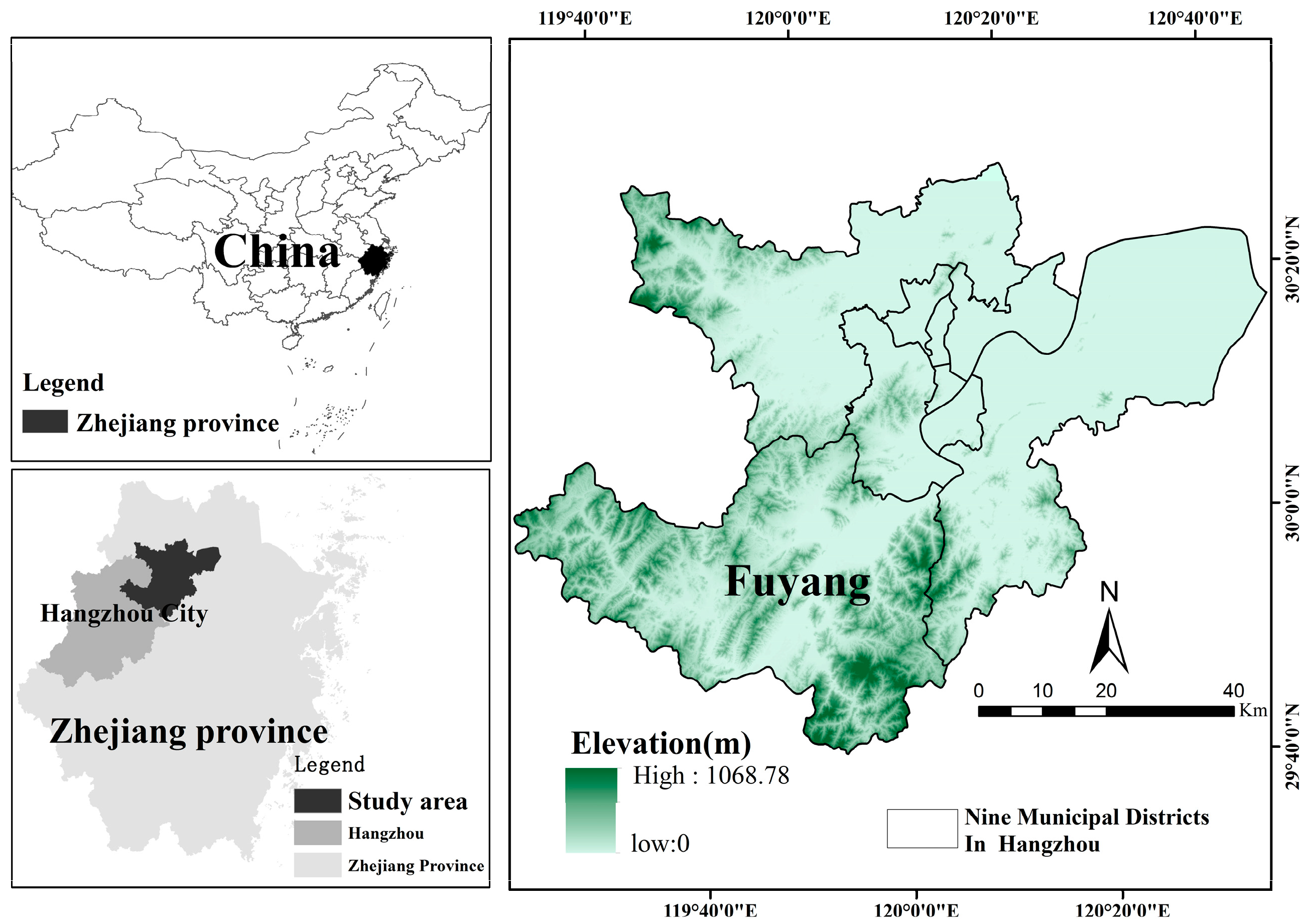
Our study area is Hangzhou (Figure 1), Eastern China, with a population of 9 million. Hangzhou is the metropolis city for Zhejiang Province, experiencing rapid urban sprawl and socio-economic development. To represent the rate of urban sprawl more directly, we only selected the nine municipal districts in Hangzhou, representing an approximate area of 4876 km2. The region covers several municipal centers with heterogeneous development activities, such as Fuyang, Yuhang district, and so on.
It is crucially important to note that the satellite city of Hangzhou (Fuyang in the southwestern part) is different from the other eight municipal districts due to its inferior socio-economic state. Therefore, the whole study area can be divided into two parts: Fuyang (the satellite city) and the other eight districts (main city). Over the past decades, the urban built-up area in Hangzhou has increased by nearly five times. This makes Hangzhou an ideal study area, as distinguishing UB will help understand the disorderly urban sprawl.
3. Methodology
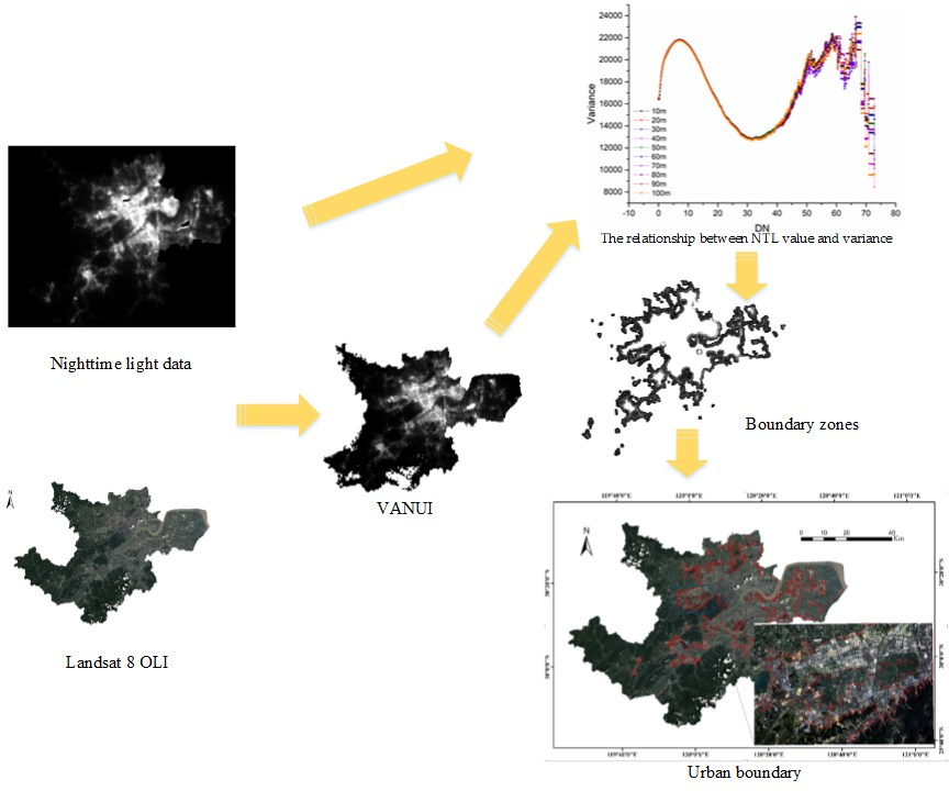
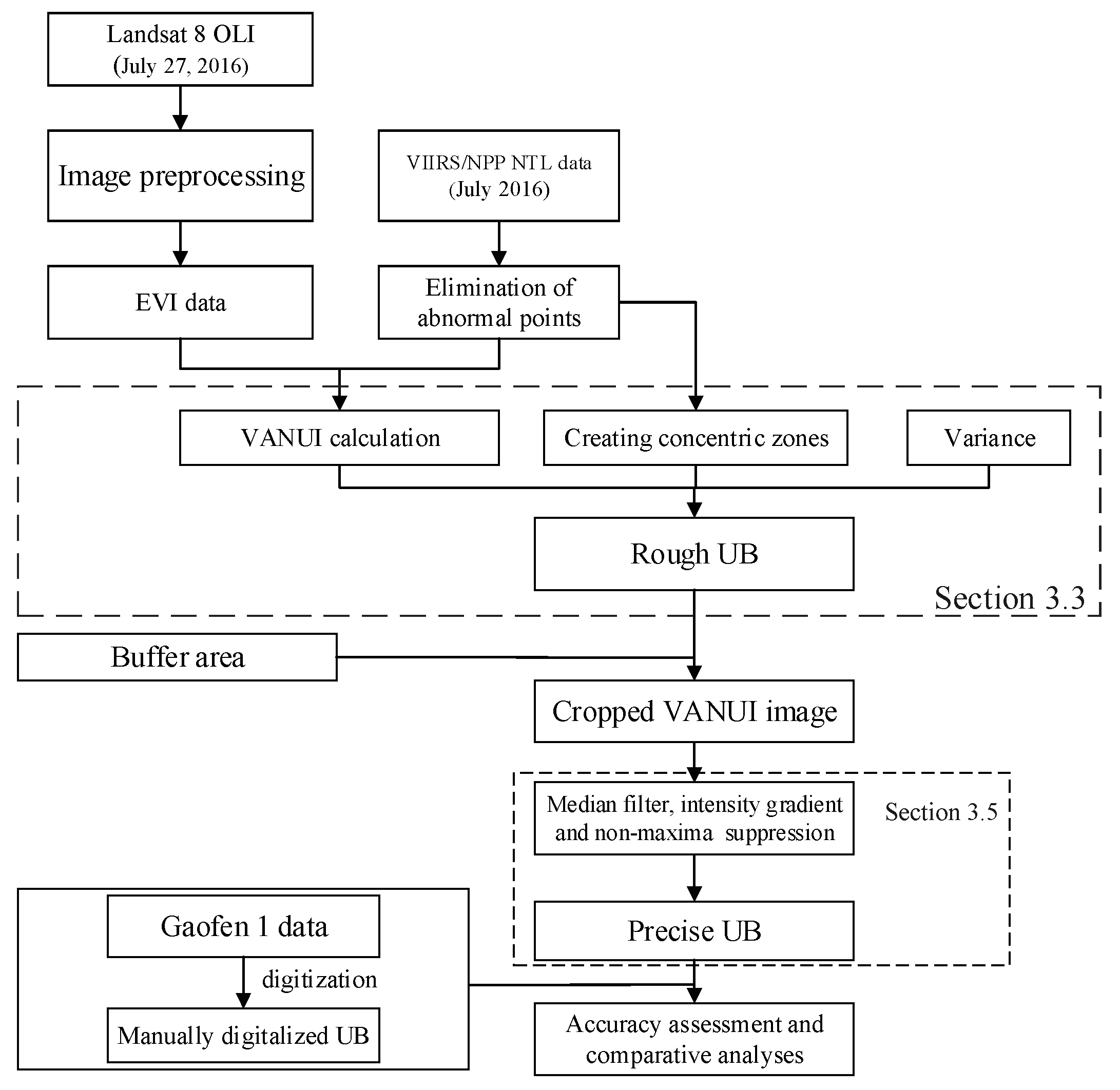
We developed a step-by-step framework to extract the UB (Figure 2) that implements a rapid, broad-scale application, whilst providing relatively accurate results. The first step was to remove the distortion in the radiance image followed by the deletion of abnormal points in the NTL data. The VANUI index was subsequently calculated, permitting the location of the rough UB by the CZM searching mode and variance-based approach. Then, an inside and outside buffer was developed along both sides of the rough UB to incorporate almost all of the blooming effect and the underestimation area. Finally, the revised edge detection method allowed for a precise and continuous UB.
3.1. Data and Image Preprocessing
Given the relatively large size of Hangzhou and the higher spectral resolution of the Landsat data compared with other high spatial resolution images, the 27 July 2016 image of Landsat 8 OLI was selected (www.earthexplorer.usgs.gov) which includes nine spectral bands (six multispectral bands, two thermal bands, and one panchromatic band). Additionally, in the summer, the flourishing vegetation makes the boundary between the urban and vegetation areas more apparent. The NPP/VIIRS NTL datum of July 2016 was obtained from the NOAA website (https://www.ngdc.noaa.gov/eog/viirs/download_dnb_composites.html). The NPP/VIIRS datum was selected because of its higher spatial (about 500 m at Hangzhou’s latitude) and radiometric (14 bit) resolution compared to the DMSP/OLS datum. The unit of NTL intensity value is nW/cm2/sr. Furthermore, the 24 July 2016 image of Gaofen1 (GF1) was selected as the reference data, which includes four multispectral bands with a spatial resolution of 8 m.
The radiometric calibration was applied to the Landsat 8 multispectral imagery and the Fast Line-of Sight Atmospheric Analysis of Spectral Hypercubes (FLAASH) software package was adopted for atmospheric correction. Both radiometric calibration and atmospheric correction were carried out using ENVI software (Exelis Visual Information Solutions., Broomfield, CO, USA), version 5.1. The released NPP/VIIRS NTL datum was not filtered to remove lights from aurora, fires, boats, and other temporal lights, so pixels with abnormal values existed in the NTL Data. Based on the previous studies, we assumed the negative digital number (DN) values were caused by the background noise and outliers from data processing. The Xiaoshan airport in the suburban area, which can easily be distinguished by its shape and size in the Landsat 8 imagery, was removed from the NTL data because, in the first place, the airport is not in the urban domain and, in the second place, the NTL intensity of the airport is excessively high compared to that of urban areas. The excessively high NTL DN in the airport would obscure the urban light. The highest NTL DN of the remaining part was 72.8 nW/cm2/sr. The position of the 72.8 nW/cm2/sr in the NTL data was in the Wulin square—one of the widely accepted urban centers in Hangzhou. Pixels with DN value less than 0 nW/cm2/sr were also removed. Following this, the NTL image was resampled to 390 m-13 fold the value of the Landsat 8 resolution through the nearest neighbor method. It ensured that an NTL pixel covered 169 Landsat 8 pixels. A Universal Transverse Mercator (UTM) projection with zone 16 and the WGS84 datum were applied to all the RS data.
3.2. VANUI: An Index for Enhancing the Variance in the Urban Pattern
The VANUI is an index proposed by Zhang et al. [29], which combines the DMSP/OLS with the NDVI derived from the MODIS data. The NTL DN decreased as the vegetation index increased from urban to rural area. In the urban fringe, both the decreasing and increasing trends were more significant and then amplified further by Equation (1). VANUI was derived from the following equation:
To obtain an improved spatial resolution product, the MODIS data was replaced by Landsat 8 OLI at a spatial resolution of 30 m. In the urban fringe, the NDVI tended to saturate along with the increasing vegetation density for the saturation effect of NDVI in high-density vegetation [29]. Therefore, we replaced the NDVI with EVI because EVI has less of a saturation effect. The NTL datum was normalized by the highest and lowest value for constraining the domain of values between 0 and 1, which have almost the same domain as the EVI. The normalized NTL was defined as follows:
Finally, the VANUI was defined as Equation (3):
VANUI = (1 − EVI) × NTL(normalized)
3.3. Deriving the Rough UB by CZM and Variance
3.3.1. Creating the Concentric Zones
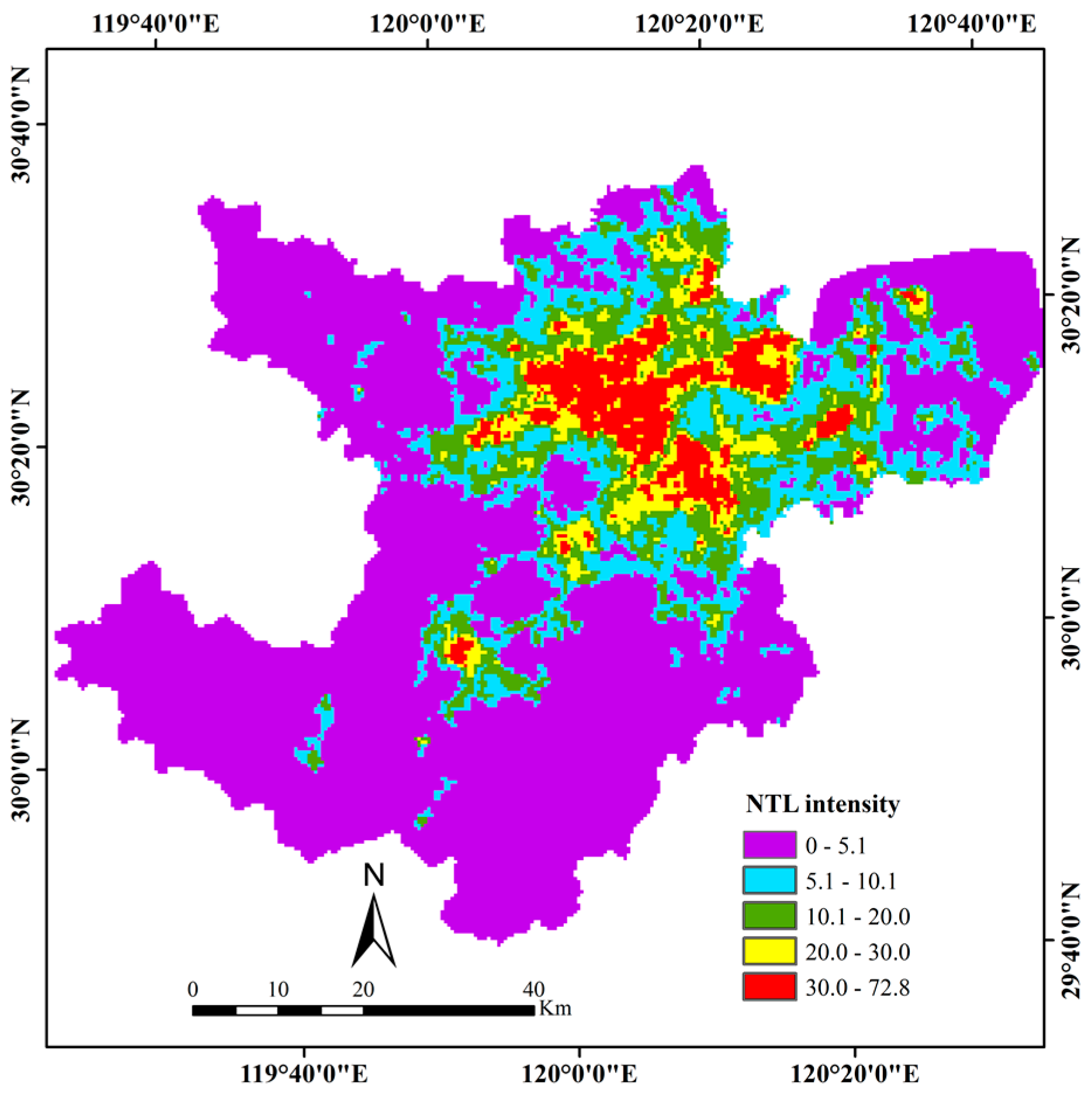
Previous studies paid less attention to the variation of NTL DN within a city, which was brought by the new generation of NTL data—NPP/VIIRS. The DMSP/OLS data cannot represent the variation owing to the saturation effect. The abrupt change points method was adopted to find the urban fringe. Regions far from urban centers with fragmented landscapes will be recognized as urban fringe [38]. In this study, we revised the search mode applied in previous studies when identifying abrupt change points. The value of the NTL data decreased from the highest to the lowest and, at the same time, established a considerable number of concentric zones (see Figure 4). The unique feature of the NTL data was called the concentric zone model. The central point of these concentric zones was the location of the highest NTL DN if the city had only one municipal center. When referring to the study area with several municipal centers, the number of central points in these concentric zones equaled the number of municipal centers. The sites of these central points were the locations of the highest NTL DN in these concentric zones, respectively.
According to the theory of CZM, the number of concentric zones was defined as follows:
Here, the denominator represents the interval of the NTL DN of two neighboring concentric zones in CZM. In our case study, we set the interval as 0.1. NTLmax and NTLmin were the highest and lowest value of NTL DN, respectively. Utilizing the CZM to search for the abrupt change points in the urban fringe provided a rapid and convenient method, compared to previous research [39].
3.3.2. Searching the Rough UB through CZM and Variance
The procedures of searching rough UB can be divided into four steps. Firstly, we clipped the VANUI image through all of the concentric zones that were established in Section 3.3.1, respectively. The times of the clippings equaled the number of concentric zones (N in Equation (4)) and were also equal to the number of the sub-regions of the VANUI image. After the clipping, we obtained N sub-regions of the VANUI image, accordingly. Taking our study area as an example, in Figure 4, the VANUI image was clipped through the concentric zone derived from the NTL DN range between 72.8 and 20 to obtain a corresponding sub-region of the VANUI image.
Secondly, the variance (V) was an effective index which represents the dispersion degree of the data, hence, we introduced it to depict the dispersion degree of these sub-regions of the VANUI image. The variance was defined as follows:
Here, N is the number of pixels in the sub-region of the VANUI image, DNi is the value of the ith pixel in the sub-region, and NTM is the mean value.
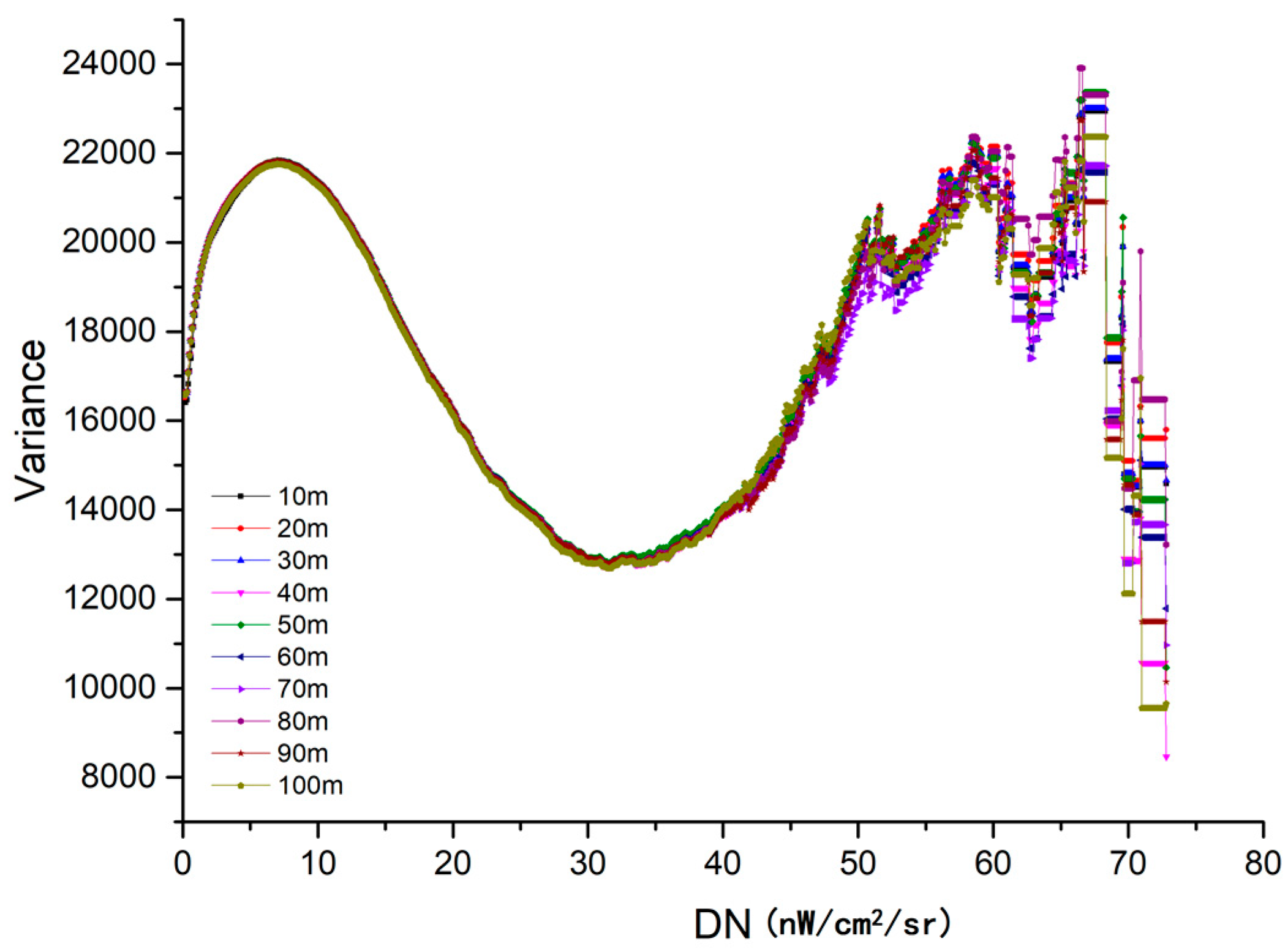
Thirdly, we attempted to find the rough extent of the urban area from rural areas to urban centers through the CZM searching mode and variance-based method. In the beginning, the first concentric zone covered the whole study area, and the outer edge of the first concentric zone was situated in pure vegetation. Taking our study area as an example (Figure 4), the first concentric zone was derived from the NTL DN range between 72.8 and 0 nW/cm2/sr. Therefore, the variance of the corresponding sub-region was low (Figure 5). Next, we reduced the area of the concentric zone by changing the NTL DN range. Taking our study area as an example, the second, third, and fourth concentric zones were derived from the NTL DN range, which correspond to 72.8 to 0.1, 72.8 to 0.2, and 72.8 to 0.3 nW/cm2/sr, respectively. The variance of the corresponding sub-regions of the VANUI image increased because the land cover situation became complex. We continued to reduce the area of the concentric zone by changing the NTL DN range until the corresponding variance of the sub-region reached the top. In our case study, the maximum variance is 21,805 (Figure 5). At this time, the outer edge of the CZM search mode touched the region with the most complex land cover situation. It was the transition zone between continuous impervious surfaces (urban) and the rural area. Hence, we reckoned that the CZM search mode reaches the rough UB. Based on the sub-region with the highest variance, we can obtain the corresponding concentric zone-rough extent of the urban area, the corresponding concentric zone was derived from the NTL DN range between 72.8 and 7.1 nW/cm2/sr in our case study. Actually, it is the process of searching for the optimized threshold on NTL data to extract the urban area. Finally, the raster feature of the rough extent was converted to a polygon feature—rough UB.
Taking our study area as an example (Figure 4), the last concentric zone was derived from the NTL DN range between 72.7 and 72.8 (interval = 0.1 nW/cm2/sr). After finishing the CZM search mode, we obtained the relationship between the variance of the sub-regions and NTL (see Figure 5). The spatial unit is a key element in determining the relationship between the variance of sub-regions and NTL. In order to make our approach more robust, the VANUI image was resampled to several different resolutions through the nearest neighbor method to test whether the relationship varies with the change of the spatial unit. We also tested whether the NTL with the highest variance varies with the spatial unit. To make the result more intuitive, we multiplied the VANUI image by 1000. All of the processes in Section 3.3 were accomplished by programming in IDL (version 8.3). Figure 5 validated the robustness of CZM search mode. We determined that the fluctuations of variance and the optimized threshold (7.1 nW/cm2/sr) did not vary with the change of spatial resolution in the VANUI image.
3.4. The Buffer Area Around the Rough UB
In Section 3.3.2, the rough UB was obtained through the corresponding concentric zone which was derived from the NTL DN range. Section 3.3.2 demonstrated the procedures for searching the optimized threshold. We reckoned that the UB required (“precise” UB) is near the rough UB within a certain distance because of the reasonable accuracy of the threshold method. Previous studies had indicated that both overestimation and underestimation of an urban area can exist even within a single city. The differences between precise UB and rough UB are the overestimation and underestimation of the urban area. Therefore, we constructed two regions along both sides of the rough UB to encompass the two areas.
As we mentioned in the introduction, most of the differences between precise UB and rough UB are overestimations and a small portion of the differences are underestimations because our study area is a megacity. The NTL DN intensity corresponded to the land cover types, such as impervious surfaces and vegetation. Therefore, we first established a region through the NTL DN range to cover the underestimation area. Based on the relationship between NTL and the variance of sub-regions (Figure 5), the upper limit of the NTL DN range is the optimized threshold because the direction of coverage is outside the rough UB. In our case study, the upper limit of the NTL DN range is always 7.1 nW/cm2/sr when establishing the region to cover the underestimation area. The area of the region was expanded by slightly reducing the lower limit of the NTL DN range until the region covered most of the underestimation area. In our study, we first set the lower limit as 7.0 and manually reduced the lower limit by 0.1 at a time (here we set interval as 0.1) until the region derived from the NTL DN range covered most of the underestimation area. Searching the other region for covering the overestimation area followed the same procedures. In our case study, the region covering the underestimation area was derived through the NTL DN range between 5.6 and 7.1, and the region covering the overestimation area was derived through the NTL DN range between 7.1 and 8.9. The whole area which includes the two regions are not a continuous space due to the characteristics of the NTL data. Hence, we established an inside and outside buffer along the rough UB to encompass the two regions. The two buffer areas together provided the whole buffer area.
3.5. Edge Detection Method to Get the Precise UB
The VANUI image was cropped by the buffer area (hereafter referred to as the cropped VANUI image). Noise reduction is a typical pre-processing step to improve the result of edge detection. Both the median filter and Gaussian filter are digital filtering techniques that are often used to remove noise from images. The Gaussian filter is a linear moving-window filter with Gaussian weight, but the median filter is a nonlinear filter. The original Gaussian filter in the Canny edge detection algorithm was replaced by the median filter. In the discussion section, the reasons for this replacement will be elaborated on. After the cropped VANUI image was filtered, the rest of the procedures of the edge extraction method generally follow the Canny algorithm [34]. The Canny edge detector is an edge detection operator that uses a multi-stage algorithm to detect a wide range of edges in image. It can extract useful structural information and reduce the amount of data to be processed. It has been widely applied in various computer vision systems. The intensity gradient (IG) was adopted to measure the spatial change in the cropped VANUI image [40]. The IG is a value for the first derivative in the horizontal direction (IGx) and the vertical direction (IGy). The IG can be determined by the following equation:
The edge direction was expressed as a value of the degree below:
Every pixel in the cropped VANUI image has a degree (angle of the ). Thus, non-maximum suppression was adopted to obtain the narrow UB. The basic principle is that the only accepted points are the local maximum in the direction of the gradient. The high and low threshold values in the Canny algorithm are empirically determined and depend on the input image so that there are no universal threshold values [34]. The debugging of the two threshold values was an attempt to try to preserve stronger edge pixels (where the pixel’s gradient value is higher than the high threshold value) for making the UB continuous and suppress the pixels that are smaller than the low threshold. The result derived from the edge detection method was a binary image. The value 1 indicated the edge information. The edge information was automatically converted to a polygon feature by the ArcScan tool in ArcGIS. The polygon feature was the precise UB that we want.
3.6. Comparative Analyses and Accuracy Assessment
There is no universally recognized UB product to validate the accuracy of our experiment. Hence, we manually delineated the UB carefully in the reference image, GF1. For one thing, the manually-digitalized UB was chosen as reference data because of the high accuracy of visual interpretation. For another, visual judgment is the optimal method to discriminate continuous urban impervious surfaces from scattered rural ones. In order to ensure the accuracy, manually-digitalized UB was carefully delineated based on the cadaster data, environment planning data, and land planning data.
Both manually-digitized UB and precise UB are line features instead of raster features. Thus, it is difficult to compare the accuracy between the two line features. We then divided the buffer area into two parts by the manually-digitalized UB, urban and non-urban. Next, the polygon feature was converted to a raster feature (raster layer 1). The same procedures were employed to the UB from our method for the subsequent accuracy assessments (raster layer 2). Raster layer 1 was selected as the ground truth image. The overall accuracy, user’s and producer’s accuracy, and the Kappa coefficient were conducted on the three regions (whole study area, the main city, and the satellite city) of raster layer 1 and layer 2, which were located in the buffer area [41]. The aim of this process was to make the accuracy assessments more meticulous and intuitive.
Section 3.3 demonstrated the procedures of searching optimized threshold to generate rough UB. We also divided the buffer area into two parts by the rough UB (NTL DN range between 7.1 and 72.8 nW/cm2/sr in our study) and then converted it to a raster feature (raster layer 3). Raster layer 1 was selected as the ground truth image. The confusion matrix was also conducted on raster layer 1 and layer 3 in order to evaluate the performance of thresholding on NTL data.
The comparative analysis with thresholding on VANUI was performed. We sampled about 200 pixels in the urban fringe for searching the optimized threshold, and the optimized threshold was set as 200 (DN value in the VANUI image) according to the statistical results. Our study area was classified into urban areas and non-urban areas according to the threshold. Using the eliminate tool in ArcGIS 10.1, the urban patches that were smaller than 1 hectare were merged with the neighboring polygon that has the longest shared border or the largest area. The aim of this procedure was to remove the fragmented urban patches in the urban fringe. After the elimination, we can get the UB. This was an UB product with a spatial resolution of 30 m. We also divided the buffer area into two parts by the UB from thresholding on VANUI and then converted it to a raster feature (raster layer 4). Raster layer 1 was selected as the ground truth image. The confusion matrix was also conducted on raster layer 1 and layer 4 in order to evaluate the performance of thresholding on VANUI data.
The comparative analysis with the object-based image analysis (OBIA) method was performed. To ignore the fragmented landscape inside the urban areas, we only conducted OBIA on the cropped VANUI image. Image segmentation was performed using the multi-resolution segmentation in eCognition Developer 9. The selection of an appropriate value of scale was the most important, since it controlled the relative size of image object. We used the “trial and error” approach to select the optimal segmentation scale parameters (SP). Firstly, we produced the image object using a small scale (5) and a large scale (40). The object was too small at 5 and was too large at 40. Then we increased the small SP and decreased the large SP until the image object fit with urban or non-urban objects. Finally, we found that the most appropriate scale was 20. Additionally, the default value of the shape and compactness were set as 0.1 and 0.5, respectively, in eCognition Developer 9. Three types of features were selected: spectral features, texture features, and geometry features. Spectral features included mean and standard deviation. Texture features included GLCM homogeneity, GLCM mean, GLCM dissimilarity, GLCM angular second moment, and GLCM entropy. Geometry features included area, length, roundness, and asymmetry. Feature space optimization (FSO) tools in eCognition were used to select the optimized features; it calculates an optimum feature combination based on selected samples. The high-resolution GF1 image was used to collect the sample data. We selected about 110 samples during this process. The nearest neighbor classifier was utilized to produce the classification result. The hierarchical structures were not explored because we only classified the cropped VANUI image into two classes: urban and non-urban. Raster layer 1 was selected as the ground truth image. The overall accuracy, user’s and producer’s accuracy, and the Kappa coefficient were conducted between raster layer 1 and the classification results from OBIA.
The visual comparisons were undertaken for comparing the UB from our method with the manually-digitalized UB by selecting two regions covered with both urban and continuous vegetation and two areas covered with both urban and rural areas, respectively.
4. Results
4.1. Delineation of the UB
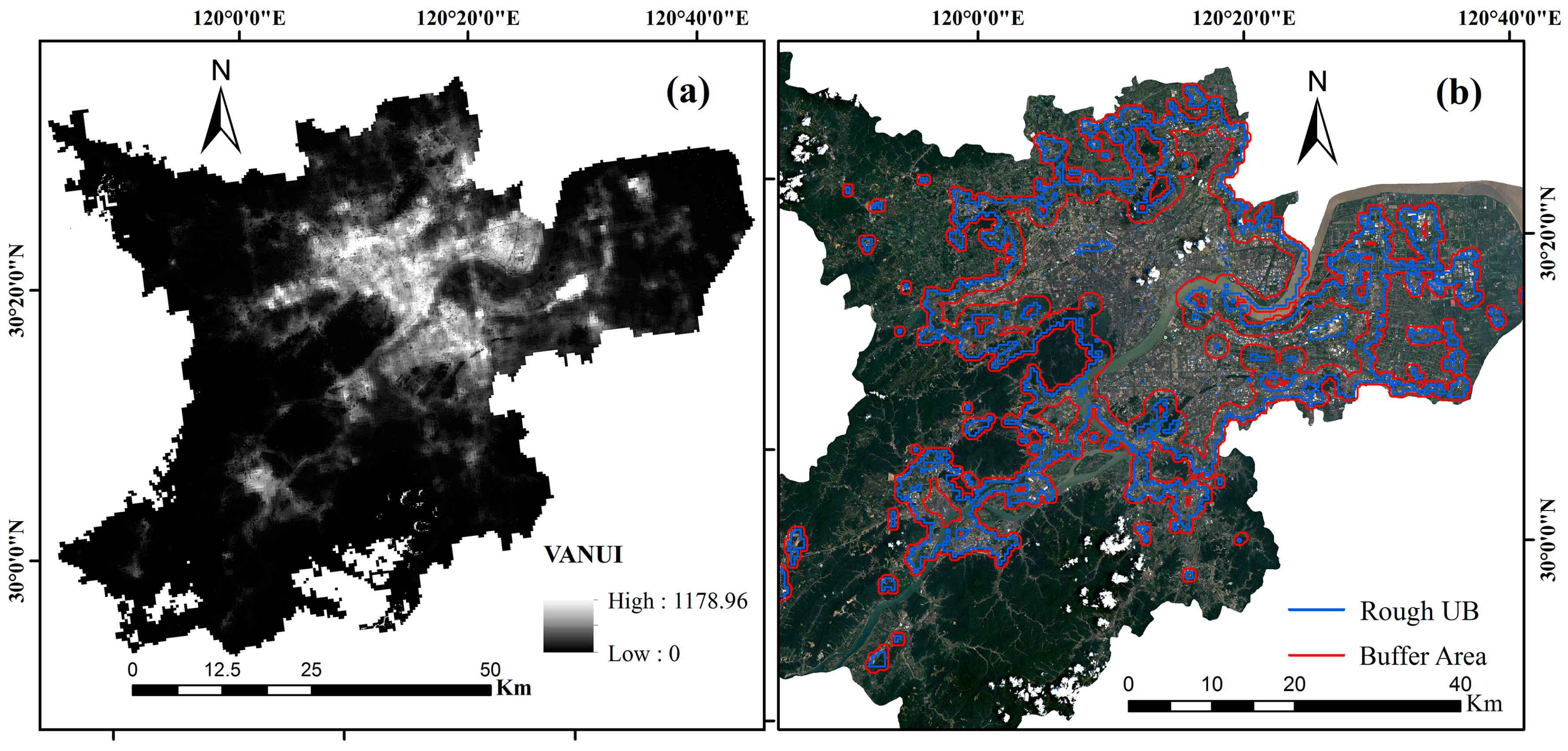
The VANUI image (DN of VANUI image multiplied by 1000) was displayed in Figure 6a. The edge information of the urban fringe was obvious. The widths of the outside and inside buffer, which was established around the rough UB, were about 390 m and 780 m, respectively (see Figure 6b). The different widths of the buffers were attributed to the characteristics of the study area (a megacity). The buffer area covered most of the overestimation and underestimation areas brought by the rough UB (threshold method).
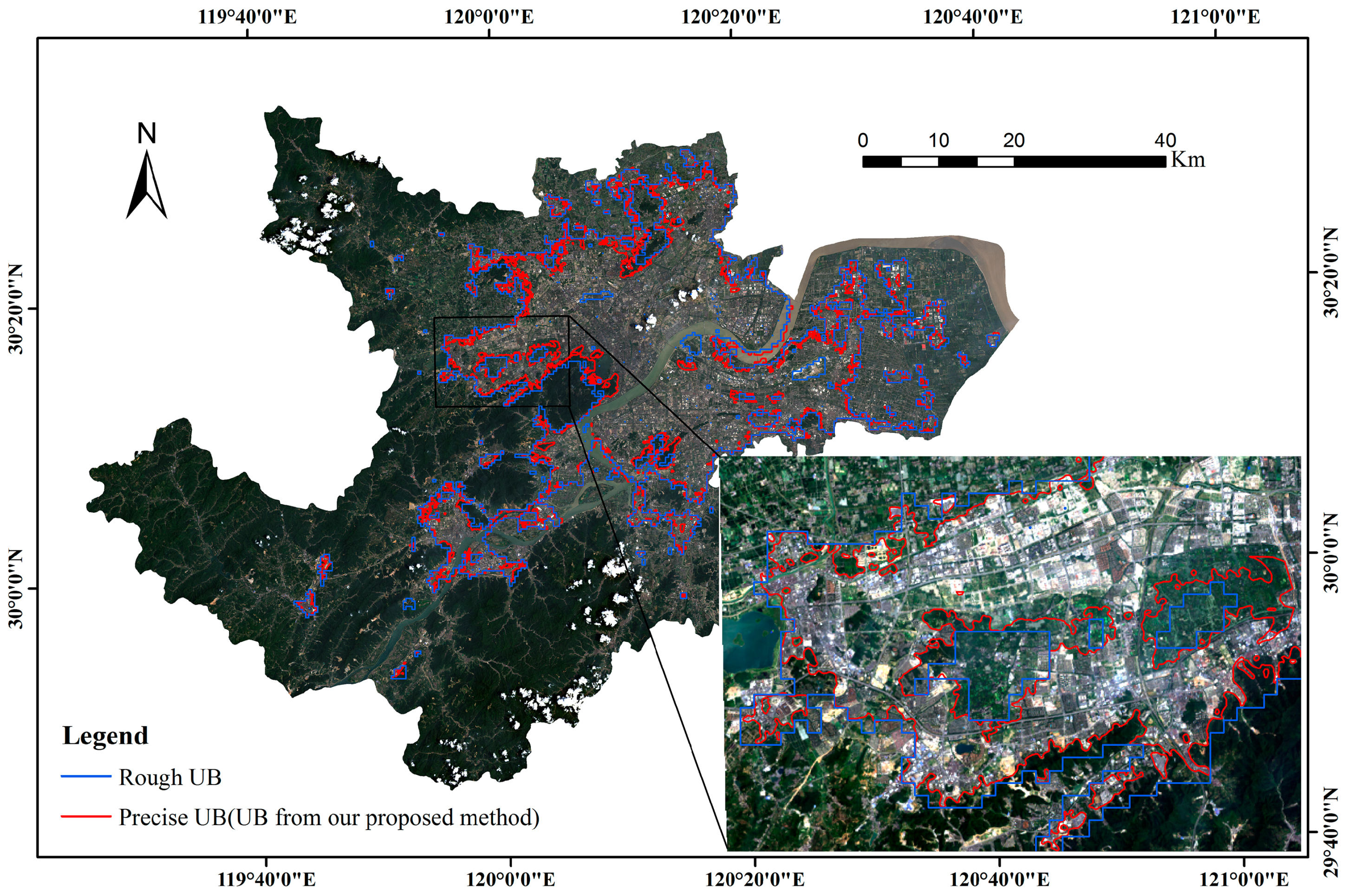
The precise UB is a product with a spatial resolution of 30 m. The urban area that consisted of most of the continuous urban impervious surfaces belonged to, and can fit into, the UB. The UB was consecutive and crosses the demarcation line between urban and continuous vegetation. In most cases, the continuous and scattered impervious surfaces were accurately separated by the precise UB (see Figure 7). The results indicated a positive result for our method. It should be noted that the UB encompassed urban green spaces and urban waters inside it. For example, the West Lake and the Qiantang River traversing Hangzhou City were urban waters in the overall urban plans of the Hangzhou government. The differences proved our point regarding the UB in Section 2.1 and indicated that deriving the UB is different from the urban impervious surfaces extraction. Some urban green space had been extracted by our method because they are situated in the buffer area.
4.2. Comparative Analyses and Accuracy Assessments
The accuracy assessments were conducted on the three regions of raster layer 1 and layer 2, which were located in the buffer area. The ability of the proposed method was confirmed with respect to the overall classification accuracies (Table 1). In general, the non-urban and urban areas achieved over 90% of the user’s accuracy and producer’s accuracy in all of the three regions, with the exception of its satellite city. The overall accuracy for the whole area was 93.87%, and even reached a higher level of 95.03% in the main city of Hangzhou, while it decreased to 87.32% in the satellite city.
In the thresholding of NTL data, the optimal threshold value was set to 7.1 nW/cm2/sr—the value for determining the rough UB in Section 3.3. We found out that the accuracy and kappa index of our method (see Table 1) far exceeded the traditional thresholding method on NTL data (see Table 2).
The urban area derived from the thresholding method on VANUI image was 1310 km2, which was approximately equal to the area of our proposed method. The overall accuracy (84.73%) was lower than that of our proposed method (93.87%). The Kappa coefficient, producer accuracy, and user accuracy of our proposed method exceeded the thresholding on the VANUI image (Table 3).
The overall accuracy of OBIA achieved 86.12% and was lower than the proposed method (93.87%). Our proposed method outperformed OBIA in the Kappa coefficient, producer accuracy, and user accuracy (Table 4).
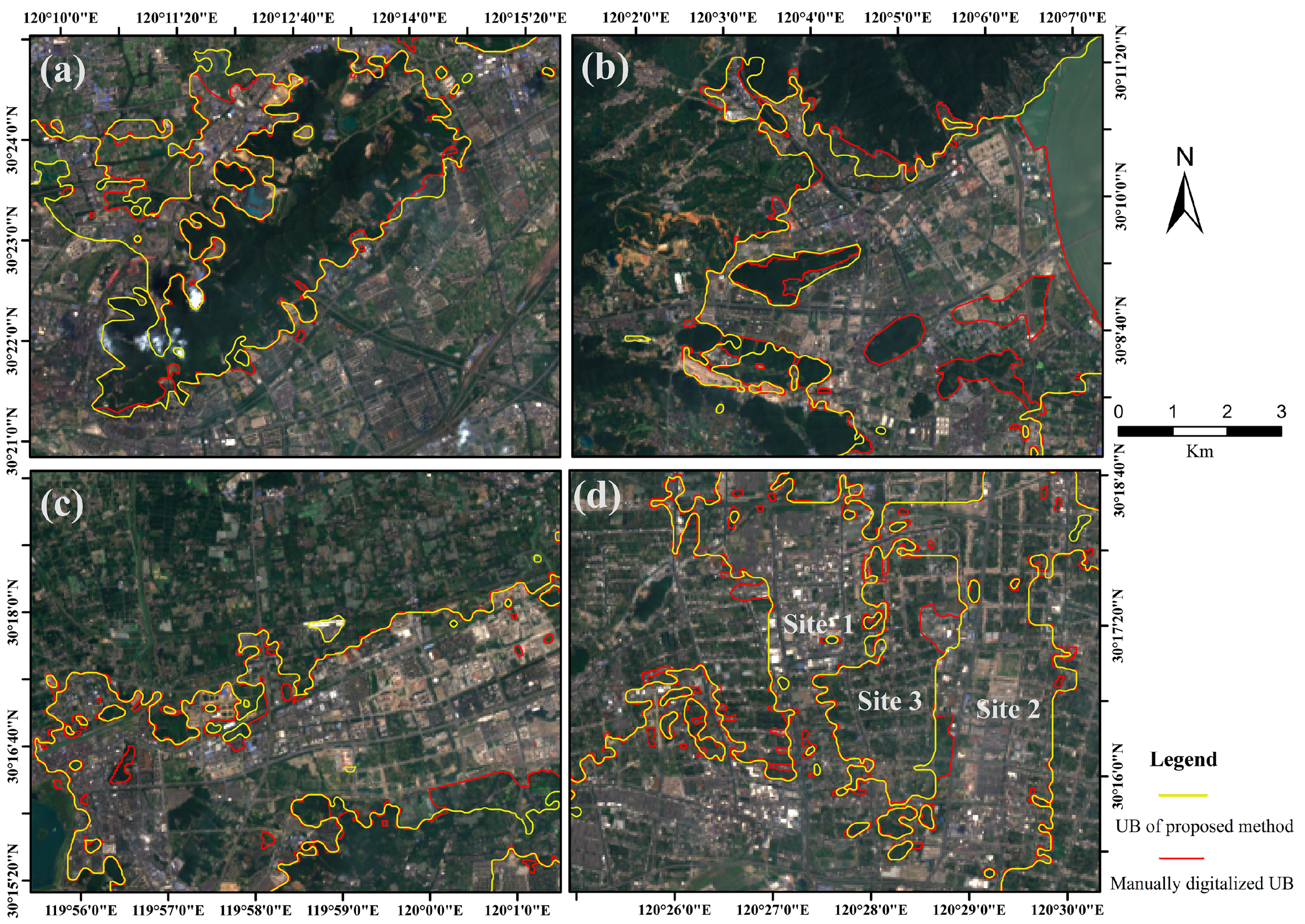
We chose two representative experimental areas to test the performance in separating continuous urban impervious surfaces from continuous vegetation. The first experimental area was the Banshan National Forest Park (Figure 8a) and the second one was located at the foot of the green hills-Westlake Scenic Spot (Figure 8b). The manually-digitalized UB (red line) overlapped with the UB from our method (yellow line) in most regions. We chose another two experimental areas to check the performance in separating continuous urban impervious surfaces from scattered rural impervious surfaces. The pattern of the rural settlements was scattered and the rural settlements usually occupied a smaller area [37]. The continuous and large areas of impervious surfaces represented the urban area. A visual comparison of the left illustration indicated that the UB between the two types of impervious surfaces was evident (Figure 8c). The pattern of the impervious surfaces became more complicated in the right illustration. Scattered impervious surfaces (site 3) resided between the two blocks of continuous impervious surfaces (site 1 and site 2). Although the boundary was blurred, our method can still delimit it (Figure 8d).
5. Discussion
5.1. The Advantages of the CZM Search Mode
Searching abrupt change points along the radius direction from urban centers to rural areas is the common method when identifying the urban extent [42]. This is known as the radius search mode in previous studies. The CZM search mode has the following advantages compared with the radius search mode: Firstly, previous studies have subjectively located the urban center by the position of the local government or the most prosperous region in the city [43]. This requires extra background knowledge about the city. In addition to this, when applying the radius search mode to cities with several municipal centers, the definition of the urban center is ambiguous. Therefore, identifying urban center(s) by the highest NTL DN is more objective. Secondly, mixed zones inside the UB consisting of urban green space, urban waters, or construction lands could be regarded as abrupt change points when applying the radius search mode to TM data. Therefore, these abnormal points should be removed through pixel-by-pixel inspections in previous studies [44]. The CZM search mode enables the abrupt change points to rest in the urban fringe. This makes the search processes more convenient compared with previous studies. Finally, calculating the variance of the VANUI image on the basis of the CZM search mode for searching the abrupt change points is more accurate than using only the attenuation rate of the NTL intensity. Hence, our method combines the advantages of NTL with Landsat 8 imagery. Moreover, the CZM search mode is more in tune with urban spatial patterns.
5.2. Replacement of the Gaussian Filter by the Median Filter
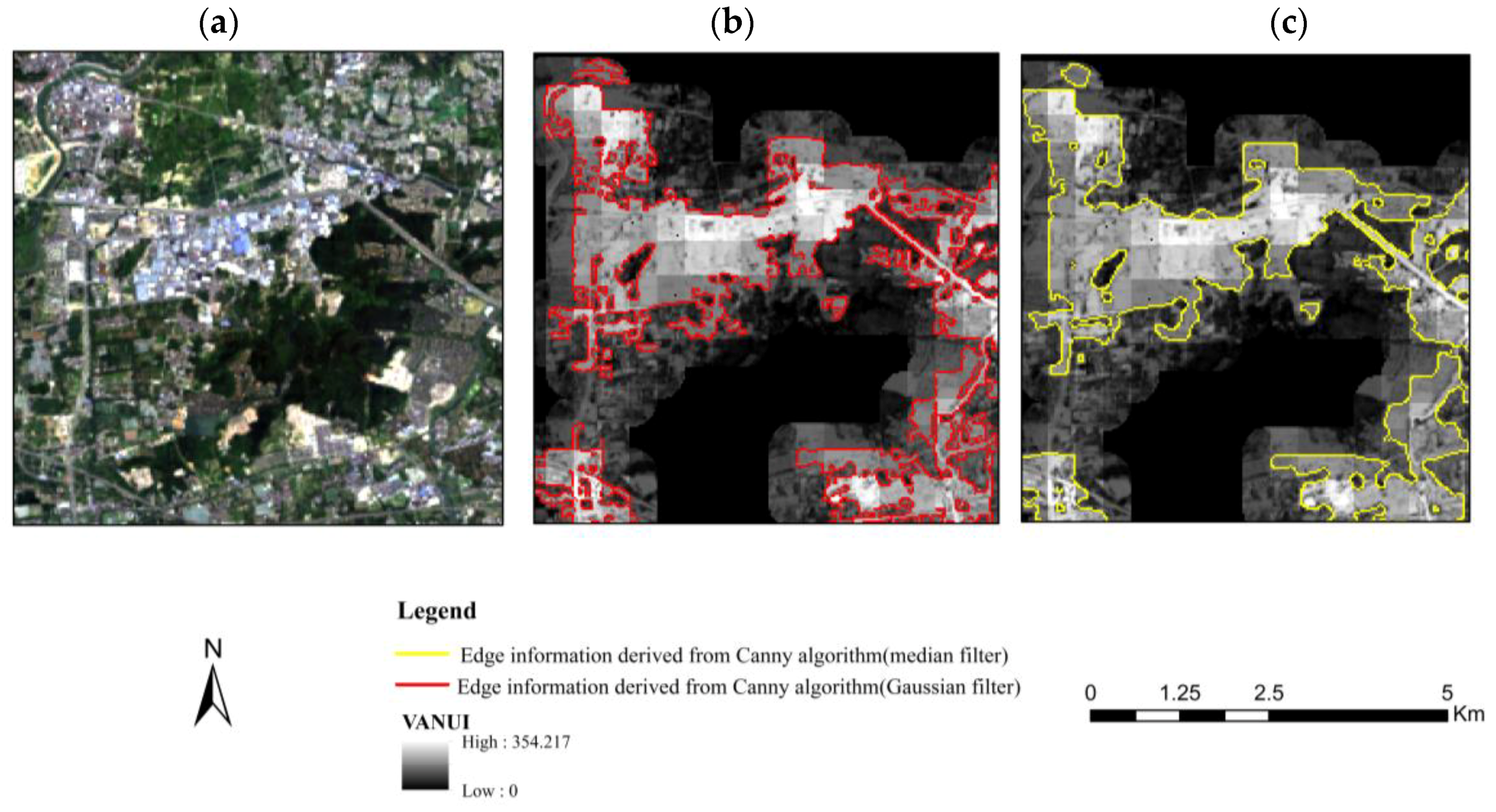
In the cropped VANUI image, the area with lower values represented vegetation and the area with higher values indicated impervious surfaces. The cropped VANUI image displayed a black and white spatial pattern, which was derived from complex spatial patterns of land covers (see Figure 9). The white points and black points had been considered as salt and pepper, respectively, in image processing. There were two types of salt and noise in the urban fringe: (1) scattered rural impervious surfaces and scattered vegetation inside the UB have a strong resemblance to the salt in the background of continuous impervious surfaces; and (2) the salt and pepper noise derived from the heterogeneity of the spectrum in the same type of land cover, such as different types of roof materials and vegetation. We regarded these types of heterogeneity as noise in the UB delineation. The median filter, a nonlinear filtering technique, is good at removing pepper, salt, and speckle noise on the basis of preserving edge-characteristics of images. The Gaussian filter blurs the information while it removes the noise. The comparison of edge information derived from the edge detection method using the two filters was displayed in Figure 9. We divided the buffer area into two parts by the UB derived from the Canny algorithm with a Gaussian filter: urban and non-urban. Then, the polygon feature was converted to a raster feature (raster layer 5). A confusion matrix in the buffer area between raster layer 1 and raster layer 5 was calculated (Table 5). The accuracy and kappa index demonstrated that the median filter outperformed the Gaussian filter because the median filter was good at removing the scattered rural impervious surfaces and the scattered vegetation inside the UB and the heterogeneity of the spectrum in the same type of land cover (see Figure 9c). After the removal, the rest of the heterogeneity information (edge information) is the UB between the urban and rural areas.
5.3. The Suitability of Our Method in Delineating UB
After acquiring the precise UB, we determined that the VANUI DN inside the UB is sometimes confused with that outside the UB (Figure 10). Taking two group of samples as an example, sample analysis was conducted on two groups: the first group comprised of site 1 and site 2, and the second group comprised of site 3 and site 4. The areas of site 1, site 2, site 3, and site 4 were 5.82 hectares, 10.64 hectares, 9.24 hectares, and 20.08 hectares, respectively. Statistical analysis showed that the maximum, minimum, and mean value of the two groups of samples are similar. A two-sample Kolmogorov-Smirnov test indicated that there were no statistically significant differences between the two groups of the samples (p value = 0.220, at the significance level of 0.05). The first two sites were covered by impervious surfaces with lower NTL intensity. However, site 3 and site 4 were vegetation- and water-filled, which reflected a large amount of NTL from the nearby buildings. Therefore, it caused the VANUI DN of the two groups of samples to be similar. This situation is very common in NTL studies and still has not been solved because DN values of NTL data recorded in a pixel equals the brightness of the illuminants in the pixel plus the brightness of the reflected NTL from nearby illuminants. However, the respective contributions are not clear so far due to the lack of a well-characterized point spread function (PSF) [25]. The edge detection method pays more attention to the edge information (the contrast among the pixels), instead of the DN value itself. Hence, it is suitable for the UB extraction from the mechanism of the edge detection method. These confusions were indirectly solved, although the mechanism of light transmission is still not clear.
There are two reasons to explain why the accuracy of the UB in Fuyang (a satellite city) is not as good as that of the main city (Table 1). For one thing, there are no lights in some settlements. Some settlements are uninhabited areas, known by the term “ghost city”. This situation makes the value of 7.1 nW/cm2/sr inaccurate. For another, the NTL intensity of cities with a high level of socio-economic development is higher than that with a low level. The Fuyang district is far less prosperous than the main city, hence, the value of 7.1 nW/cm2/sr is mainly the NTL DN of the urban fringe of the main city rather than the Fuyang district. After adopting our method to only the Fuyang district, the true value of the urban fringe in the Fuyang district is 4.3 nW/cm2/sr, which is far less than 7.1 nW/cm2/sr. Moreover, as we mentioned in the introduction, a uniform regional threshold would result in the overestimation of large cities and the underestimation of small cities. Therefore, the width of the outside buffer should be larger than that of the inside buffer when applying our method to Fuyang because it is a small city. However, in our experiment, the two buffer widths were opposite. Some scholars divided their study area into several regions with similar socio-economic development characteristics to avoid this mistake for searching the local optimal threshold [6,45]. The level of social development could easily be acquired through government reports. Cities with similar levels of social development can be processed together when applying our method to a broad-scale application. If the study areas are all megacities, most of the differences between rough UB and precise UB are overestimations. If the study areas are all small cities, most of the differences are underestimations. This way, it will be easier to find the buffer area.
There are a few limitations to our proposed approach. For example, in megacities, the DMSP/OLS NTL data cannot be applied to our method due to the saturation effect. The CZM search mode cannot be constructed because the NTL DN of the entire urban area in megacities usually reaches the saturation value. Therefore, our method has to focus on the extraction of UB after 2012. Moreover, the buffer area was established through manual work and, thus, it reduces the transferability of our method. In future studies, we will test some methods for the automatic extraction of the buffer area. Fuzzy sets, rough sets, and entropy represent the uncertainty and randomness of the land covers near rough UB. These mathematical tools provide potential for further improving the extraction of the buffer area in the future. The availability of high spatial resolution NTL data from satellites, such as Jilin-1 from China, represent a valuable source of information on spatial patterns of cities at night [46,47]. It is expected to improve the performance of our approach.
6. Conclusions
In this study, we combined the advantages of nighttime and daytime data for delimiting the UB, which is a concept that is different from urban impervious surface extraction. The NPP/VIIRS NTL data is good at mapping the rough extent of the urban area. Furthermore, the Landsat 8 data can provide the detailed edge information in the urban fringe as well. CZM, a model based on the attenuation characteristic of NTL data, and a variance-based approach were established for the rough UB and then we refined them using an edge detection method. CZM makes the abrupt change points rest in the urban fringe which is more convenient than the radius search mode in the previous UB delineating studies. The relationship between NTL and variance did not change under different spatial units of the VANUI images. The edge detection method proved to be suitable to derive UB. Our method can be applied to different types of cities, such as polycentric and monocentric cities.
The total urban area of Hangzhou from our proposed method is 1242 km2, which is 179 km2 less than the global-fixed threshold method on NTL data and is 68 km2 less than the thresholding on the VANUI image. Comparative analyses and accuracy assessments confirmed that our method is as satisfactory as manually digitalizing UB, with an overall accuracy of 93.87%. Our method is especially suitable for UB extraction and successfully tackles the issues of the blooming effect and the underestimation brought on by the inherent flaws of NTL data. Therefore, the spatial application field of NTL has been expanded to the local scale. There is no need to manually delineate UB and the simplicity of this method makes it promising for regularly monitoring and inspecting the urban development once the Chinese government implements the UB management system.
Author Contributions
X.X. designed the study and methodology; S.Z. and H.X. carried out the experimental design; Q.Z. and Z.Y. analyzed the data; K.W. proposed the idea of the urban boundary and designed the structure of this manuscript; M.G. provided suggestions on the precision evaluation in this study; and M.W. helped revise the manuscript. All authors approved the final manuscript.
Acknowledgments
This study was financially supported by the National Natural Science Foundation of China (grant no. 41701171), the Natural Science Foundation of Zhejiang Province of China (grant no. LQ17D010003), and the Basic Public Welfare Research Program of Zhejiang Province (no. LGN18D010002). We would like to gratefully thank the anonymous reviewers and editors for their insightful and helpful comments to improve the manuscript.
Conflicts of Interest
The authors declare no conflict of interest.
References
- Miller, M.D. The impacts of Atlanta’s urban sprawl on forest cover and fragmentation. Appl. Geogr. 2012, 34, 171–179. [Google Scholar] [CrossRef]
- He, C.; Liu, Z.; Tian, J.; Ma, Q. Urban expansion dynamics and natural habitat loss in China: A multiscale landscape perspective. Glob. Chang. Biol. 2014, 20, 2886–2902. [Google Scholar] [CrossRef] [PubMed]
- Bhatta, B.; Saraswati, S.; Bandyopadhyay, D. Urban sprawl measurement from remote sensing data. Appl. Geogr. 2010, 30, 731–740. [Google Scholar] [CrossRef]
- Mulligan, G.F. Revisiting the urbanization curve. Cities 2013, 32, 113–122. [Google Scholar] [CrossRef]
- Pan, Y.; Marshall, S.; Maltby, L. Prioritising ecosystem services in Chinese rural and urban communities. Ecosyst. Serv. 2016, 21, 1–5. [Google Scholar] [CrossRef]
- Xiao, P.; Wang, X.; Feng, X.; Zhang, X.; Yang, Y. Detecting China’s urban expansion over the past three decades using nighttime light data. IEEE J. Sel. Top. Appl. Earth Obs. Remote Sens. 2014, 7, 4095–4106. [Google Scholar] [CrossRef]
- Huang, X.; Lu, Q.; Zhang, L. A multi-index learning approach for classification of high-resolution remotely sensed images over urban areas. ISPRS J. Photogramm. Remote Sens. 2014, 90, 36–48. [Google Scholar] [CrossRef]
- Goldblatt, R.; You, W.; Hanson, G.; Khandelwal, A.K. Detecting the boundaries of urban areas in India: A dataset for pixel-based image classification in google earth engine. Remote Sens. 2016, 8, 634. [Google Scholar] [CrossRef]
- Duro, D.C.; Franklin, S.E.; Dubé, M.G. A comparison of pixel-based and object-based image analysis with selected machine learning algorithms for the classification of agricultural landscapes using SPOT-5 HRG imagery. Remote Sens. Environ. 2012, 118, 259–272. [Google Scholar] [CrossRef]
- Xu, H. Analysis of Impervious Surface and its Impact on Urban Heat Environment using the Normalized Difference Impervious Surface Index (NDISI). Photogramm. Eng. Remote Sens. 2010, 76, 557–565. [Google Scholar] [CrossRef]
- Bhatti, S.S.; Tripathi, N.K. Built-up area extraction using Landsat 8 OLI imagery. GIScience Remote Sens. 2014, 51, 445–467. [Google Scholar] [CrossRef]
- Estoque, R.C.; Murayama, Y. Classification and change detection of built-up lands from Landsat-7 ETM+ and Landsat-8 OLI/TIRS imageries: A comparative assessment of various spectral indices. Ecol. Indic. 2015, 56, 205–217. [Google Scholar] [CrossRef]
- Yu, B.; Shi, K.; Hu, Y.; Huang, C.; Chen, Z.; Wu, J. Poverty Evaluation Using NPP-VIIRS Nighttime Light Composite Data at the County Level in China. IEEE J. Sel. Top. Appl. Earth Obs. Remote Sens. 2015, 8, 1217–1229. [Google Scholar] [CrossRef]
- Letu, H.; Hara, M.; Yagi, H.; Naoki, K.; Tana, G.; Nishio, F.; Shuhei, O. Estimating energy consumption from night-time DMPS/OLS imagery after correcting for saturation effects. Int. J. Remote Sens. 2010, 31, 4443–4458. [Google Scholar] [CrossRef]
- Deville, P.; Linard, C.; Martin, S.; Gilbert, M.; Stevens, F.R.; Gaughan, A.E.; Blondel, V.D.; Tatem, A.J.; Chen, X.; Nordhaus, W.D. Using luminosity data as a proxy for economic statistics. Proc. Natl. Acad. Sci. USA 2014, 108, 8589–8594. [Google Scholar] [CrossRef]
- Small, C.; Pozzi, F.; Elvidge, C.D. Spatial analysis of global urban extent from DMSP-OLS night lights. Remote Sens. Environ. 2005, 96, 277–291. [Google Scholar] [CrossRef]
- Elvidge, C.D.; Sutton, P.C.; Ghosh, T.; Tuttle, B.T.; Baugh, K.E.; Bhaduri, B.; Bright, E. A global poverty map derived from satellite data. Comput. Geosci. 2009, 35, 1652–1660. [Google Scholar] [CrossRef]
- Sharma, R.C.; Tateishi, R.; Hara, K.; Gharechelou, S.; Iizuka, K. Global mapping of urban built-up areas of year 2014 by combining MODIS multispectral data with VIIRS nighttime light data. Int. J. Digit. Earth 2016, 9, 1004–1020. [Google Scholar] [CrossRef]
- Cao, X.; Chen, J.; Imura, H.; Higashi, O. A SVM-based method to extract urban areas from DMSP-OLS and SPOT VGT data. Remote Sens. Environ. 2009, 113, 2205–2209. [Google Scholar] [CrossRef]
- Li, B.; Ti, C.; Zhao, Y.; Yan, X. Estimating soil moisture with Landsat data and its application in extracting the spatial distribution of winter flooded paddies. Remote Sens. 2016, 8. [Google Scholar] [CrossRef]
- Zhang, X.; Li, P.; Cai, C. Regional urban extent extraction using multi-sensor data and one-class classification. Remote Sens. 2015, 7, 7671–7694. [Google Scholar] [CrossRef]
- Amaral, S.; Câmara, G.; Monteiro, A.M.V.; Quintanilha, J.A.; Elvidge, C.D. Estimating population and energy consumption in Brazilian Amazonia using DMSP night-time satellite data. Comput. Environ. Urban Syst. 2005, 29, 179–195. [Google Scholar] [CrossRef]
- Henderson, M.; Yeh, E.T.; Gong, P.; Elvidge, C.; Baugh, K. Validation of urban boundaries derived from global night-time satellite imagery. Int. J. Remote Sens. 2003, 24, 595–609. [Google Scholar] [CrossRef]
- Li, B.-L.; Ti, C.-P.; Yan, X.-Y. Estimating rice paddy areas in China using multi-temporal cloud-free NDVI imagery based on change detection. Pedosphere 2017. [Google Scholar] [CrossRef]
- Zhou, Y.; Smith, S.J.; Elvidge, C.D.; Zhao, K.; Thomson, A.; Imhoff, M. A cluster-based method to map urban area from DMSP/OLS nightlights. Remote Sens. Environ. 2014, 147, 173–185. [Google Scholar] [CrossRef]
- Tan, M. Use of an inside buffer method to extract the extent of urban areas from DMSP/OLS nighttime light data in North China. GIScience Remote Sens. 2016, 53, 444–458. [Google Scholar] [CrossRef]
- Kyba, C.C.M.; Wagner, J.M.; Kuechly, H.U.; Walker, C.E.; Elvidge, C.D.; Falchi, F.; Ruhtz, T.; Fischer, J.; Hölker, F. Citizen science provides valuable data for monitoring global night sky luminance. Sci. Rep. 2013, 3. [Google Scholar] [CrossRef] [PubMed]
- Ouyang, Z.; Fan, P.; Chen, J. Urban Built-up Areas in Transitional Economies of Southeast Asia: Spatial Extent and Dynamics. Remote Sens. 2016, 8, 819. [Google Scholar] [CrossRef]
- Zhang, Q.; Schaaf, C.; Seto, K.C. The Vegetation adjusted NTL Urban Index: A new approach to reduce saturation and increase variation in nighttime luminosity. Remote Sens. Environ. 2013, 129, 32–41. [Google Scholar] [CrossRef]
- Su, Y.; Chen, X.; Wang, C.; Zhang, H.; Liao, J.; Ye, Y.; Wang, C. A new method for extracting built-up urban areas using DMSP-OLS nighttime stable lights: A case study in the Pearl River Delta, southern China. GIScience Remote Sens. 2015, 1603, 1–21. [Google Scholar] [CrossRef]
- Li, Q.; Lu, L.; Weng, Q.; Xie, Y.; Guo, H. Monitoring urban dynamics in the Southeast U.S.A. using time-series DMSP/OLS nightlight imagery. Remote Sens. 2016, 8, 13–15. [Google Scholar] [CrossRef]
- Bachofer, F.; Quénéhervé, G.; Märker, M. The delineation of paleo-shorelines in the lake manyara basin using terraSAR-X data. Remote Sens. 2014, 6, 2195–2212. [Google Scholar] [CrossRef]
- Liu, H.; Jezek, K.C. Automated extraction of coastline from satellite imagery by integrating Canny edge detection and locally adaptive thresholding methods. Int. J. Remote Sens. 2004, 25, 937–958. [Google Scholar] [CrossRef]
- Canny, J. A Computational Approach to Edge Detection. IEEE Trans. Pattern Anal. Mach. Intell. 1986, PAMI-8, 679–698. [Google Scholar] [CrossRef] [PubMed]
- Liu, Z.; He, C.; Zhou, Y.; Wu, J. How much of the world’s land has been urbanized, really? A hierarchical framework for avoiding confusion. Landsc. Ecol. 2014, 29, 763–771. [Google Scholar] [CrossRef]
- Wu, J. Urban ecology and sustainability: The state-of-the-science and future directions. Landsc. Urban Plan. 2014, 125, 209–221. [Google Scholar] [CrossRef]
- Zheng, X.; Wang, Y.; Gan, M.; Zhang, J.; Teng, L.; Wang, K.; Shen, Z.; Zhang, L. Discrimination of settlement and industrial area using landscape metrics in rural region. Remote Sens. 2016, 8. [Google Scholar] [CrossRef]
- Murgante, B.; Las Casas, G.; Sansone, A.; Basilicata, U. A spatial rough set for locating the periurban fringe. In Proceedings of the SAGEO 2007: Colloque International de Géomatique et d’Analyse Spatiale, Saint-Etienne, France, 18–22 June 2007. [Google Scholar]
- Ju, C.; Zhou, X.; He, Q. On the application of a concentric zone model (CZM) for classifying and extracting urban boundaries using night-time stable light data in Urumqi of Xinjiang, China. Remote Sens. Lett. 2016, 7, 1033–1042. [Google Scholar] [CrossRef]
- Tan, M. An Intensity Gradient/Vegetation Fractional Coverage Approach to Mapping Urban Areas from DMSP/OLS Nighttime Light Data. IEEE J. Sel. Top. Appl. Earth Obs. Remote Sens. 2017, 10, 95–103. [Google Scholar] [CrossRef]
- Congalton, R.G. A Review of Assessing the Accuracy of Classification of Remotely Sensed Data a Review of Assessing the Accuracy of Classifications of Remotely Sensed Data. Remote Sens. Environ. 1991, 4257, 34–46. [Google Scholar] [CrossRef]
- Ma, T.; Zhou, Y.; Zhou, C.; Haynie, S.; Pei, T.; Xu, T. Night-time light derived estimation of spatio-temporal characteristics of urbanization dynamics using DMSP/OLS satellite data. Remote Sens. Environ. 2015, 158, 453–464. [Google Scholar] [CrossRef]
- Moura, K.; Neto, R.S. Individual and contextual determinants of victimisation in Brazilian urban centres: A multilevel approach. Urban Stud. 2016, 53, 1559–1573. [Google Scholar] [CrossRef]
- Hu, S.; Tong, L.; Frazier, A.E.; Liu, Y. Urban boundary extraction and sprawl analysis using Landsat images: A case study in Wuhan, China. Habitat Int. 2015, 47, 183–195. [Google Scholar] [CrossRef]
- Liu, Z.; He, C.; Zhang, Q.; Huang, Q.; Yang, Y. Extracting the dynamics of urban expansion in China using DMSP-OLS nighttime light data from 1992 to 2008. Landsc. Urban Plan. 2012, 106, 62–72. [Google Scholar] [CrossRef]
- Levin, N.; Johansen, K.; Hacker, J.M.; Phinn, S. A new source for high spatial resolution night time images—The EROS-B commercial satellite. Remote Sens. Environ. 2014, 149, 1–12. [Google Scholar] [CrossRef]
- Levin, N.; Duke, Y. High spatial resolution night-time light images for demographic and socio-economic studies. Remote Sens. Environ. 2012, 119, 1–10. [Google Scholar] [CrossRef]
Figure 1.
The location of the study area.

Figure 2.
The framework proposed for this study.

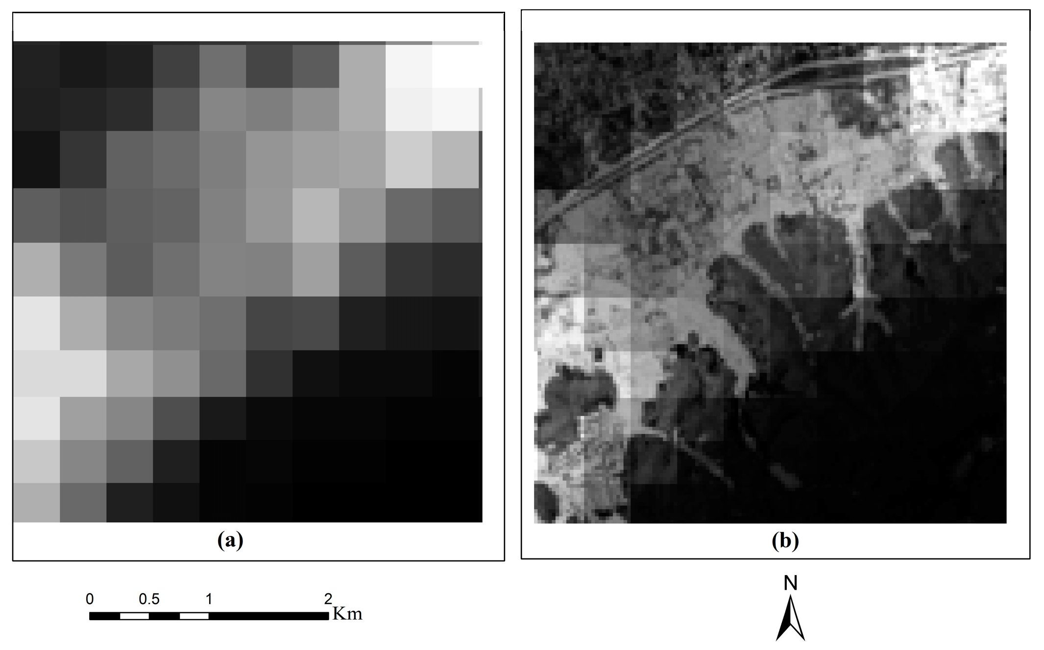
Figure 3.
The schematic diagram showing the nighttime light (NTL) data (a) and the VANUI (b). The spatial resolutions of these are 390 m and 30 m, respectively.
Figure 3.
The schematic diagram showing the nighttime light (NTL) data (a) and the VANUI (b). The spatial resolutions of these are 390 m and 30 m, respectively.

Figure 4.
This diagram takes the study area with several municipal centers as an example to illustrate the principle of the concentric zone model (CZM). In our study, 728 concentric zones were established (interval = 0.1 nW/cm2/sr). Taking two concentric zones, for the example, the red part represents the concentric zone derived from the NTL digital number (DN) range between 72.8 (the highest NTL DN of the study area) and 30 nW/cm2/sr. The red and the yellow parts represent another concentric zone derived from the NTL DN range between 72.8 and 20 nW/cm2/sr.

Figure 5.
An intermediate result of our method which indicated the relationship between NTL intensity and variance between rural and urban areas. The variances were calculated from the sub-regions of the VANUI image, which were clipped by corresponding concentric zones. The concentric zones were derived from the corresponding NTL DN range. The 10–100 m range represented the different spatial resolutions of the VANUI images after resampling.

Figure 6.
(a) The VANUI image (multiplied by 1000), and (b) the rough UB and buffer area, the 27 July 2016 image of Landsat 8 OLI in Section 3.1 was selected as the background satellite image.
Figure 6.
(a) The VANUI image (multiplied by 1000), and (b) the rough UB and buffer area, the 27 July 2016 image of Landsat 8 OLI in Section 3.1 was selected as the background satellite image.

Figure 7.
The precise UB and the rough UB; the 27 July 2016 image of Landsat 8 OLI in Section 3.1 was selected as the background satellite image.
Figure 7.
The precise UB and the rough UB; the 27 July 2016 image of Landsat 8 OLI in Section 3.1 was selected as the background satellite image.

Figure 8.
The comparisons of the two UBs in the mixed zones between continuous vegetation and continuous impervious surfaces ((a,b), respectively). The comparisons of the two UBs in the mixed zones between the scattered and continuous impervious surfaces ((c,d), respectively). The boundary line in red is the manually-digitalized UB and the yellow boundary line is from the proposed method. The 27 July 2016 image of the Landsat 8 OLI in Section 3.1 was selected as the background satellite image. The descriptions of the manually-digitalized UB can be found in the Methodology section (Section 3.6).

Figure 9.
The comparison between the median and Gaussian filter in removing the salt and pepper noise. (a) Landsat 8 OLI 30 m true color image; (b) the edge information derived from the Canny algorithm with a Guassian filter; and (c) the edge information formed by the Canny algorithm with a median filter. The VANUI image was selected as the background image.

Figure 10.
Taking two groups of samples as an example to illustrate the confusion among the VANUI values inside and outside the UB. Site 1 and site 2 were covered by impervious surfaces with lower NTL intensity, and site 3 and site 4 were vegetation- and water-filled, which reflected a large amount of NTL from nearby buildings. The VANUI DN of the first group of lower NTL values were confused with the second group of high NTL value. The VANUI image was selected as the background image.


Table 1.
The confusion matrix between raster layer 1 and raster layer 2.
| Whole Study Area | Main City | Fuyang (Satellite City) | ||||||||||
|---|---|---|---|---|---|---|---|---|---|---|---|---|
| Non- Urban | Urban | Prod. Acc. | User. Acc. | Non- Urban | Urban | Prod. Acc. | User. Acc. | Non- Urban | Urban | Prod. Acc. | User. Acc. | |
| Non- Urban | 673,623 | 20,786 | 91.67% | 97.01% | 558,524 | 11,382 | 92.56% | 98.00% | 112,308 | 9385 | 87.33% | 92.29% |
| Urban | 61,237 | 582,658 | 96.56% | 90.49% | 44,896 | 528,470 | 97.85% | 92.01% | 16,298 | 64,541 | 87.30% | 79.84% |
| Kappa | 0.877 | 0.9005 | 0.7318 | |||||||||
| Over.Acc. | 93.87% | 95.03% | 87.32% | |||||||||
Note: Raster layer 1 is a raster feature which was produced by the manually-digitalized UB (vector features). Raster layer 2 is a raster layer which was produced by the precise UB (vector features). The buffer area was divided into two parts by the manually-digitalized UB, urban and non-urban, and then the polygon feature was converted to a raster feature (raster layer 1). The same procedures were employed to the precise UB to get the raster layer 2. Raster layer 1 was selected as the ground truth image.
Table 2.
The confusion matrix between raster layer 1 and raster layer 3.
| Non-Urban | Urban | Prod. Acc | User. Acc | |
|---|---|---|---|---|
| Non-urban | 462,913 | 29,434 | 62.99% | 94.02% |
| Urban | 271,947 | 574,010 | 95.12% | 67.85% |
| Kappa | 0.5610 | |||
| Over.Acc | 77.48% | |||
Note: Raster layer 1 is a raster feature which was produced by the manually-digitalized UB (vector features). Raster layer 3 is a raster layer which was produced by the UB from thresholding of NTL data (vector features). The buffer area was divided into two parts by the manually-digitalized UB, urban and non-urban. Then the polygon feature was converted to a raster feature (raster layer 1). The same procedures were employed to the UB from thresholding of NTL data to obtain raster layer 3. Raster layer 1 was selected as the ground truth image.
Table 3.
The confusion matrix between raster layer 1 and raster layer 4.
| Non-Urban | Urban | Prod. Acc | User. Acc | |
|---|---|---|---|---|
| Non-urban | 589,853 | 66,048 | 81.23% | 89.93% |
| Urban | 136,312 | 533,429 | 88.98% | 79.65% |
| Kappa | 0.6950 | |||
| Over.Acc | 84.73% | |||
Note: Raster layer 1 is a raster feature which was produced by the manually-digitalized UB (vector features). Raster layer 4 is a raster layer which was produced by the UB from thresholding of VANUI data (vector features). The buffer area was divided into two parts by the manually-digitalized UB, urban and non-urban. Then the polygon feature was converted to a raster feature (raster layer 1). The same procedures were employed to the UB from thresholding of the VANUI image to obtain raster layer 4. Raster layer 1 was selected as the ground truth image.
Table 4.
The Confusion matrix between raster layer1 and classification results from OBIA.
| Non-Urban | Urban | Prod. Acc | User. Acc | |
|---|---|---|---|---|
| Non-urban | 611,676 | 69,502 | 84.23% | 89.80% |
| urban | 114,479 | 529,975 | 88.41% | 82.24% |
| kappa | 0.7217 | |||
| over.acc | 86.12% | |||
Note: Raster layer 1 is a raster feature which was produced by the manually-digitalized UB (vector features). The buffer area was divided into two parts by the manually-digitalized UB, urban and non-urban. Then the polygon feature was converted to raster feature (raster layer 1).
Table 5.
The confusion matrix between raster layer 1 and raster layer 5.
| Non-Urban | Urban | Prod. Acc. | User. Acc. | |
|---|---|---|---|---|
| Non-Urban | 614,015 | 40,398 | 84.58% | 93.83% |
| Urban | 111,931 | 559,610 | 93.27% | 83.33% |
| Kappa | 0.7705 | |||
| Over. Acc. | 88.51% | |||
Note: Raster layer 1 is a raster feature which was produced by the manually-digitalized UB (vector features). Raster layer 5 is a raster layer which was produced by the UB derived from the Canny algorithm with a Gaussian filter (vector features). The buffer area was divided into two parts by the manually-digitalized UB: urban and non-urban, and then the polygon feature was converted to the raster feature (raster layer 1). The same procedures were employed to the UB derived from the Canny algorithm with a Gaussian filter to obtain raster layer 5. Raster layer 1 was selected as the ground truth image.
© 2018 by the authors. Licensee MDPI, Basel, Switzerland. This article is an open access article distributed under the terms and conditions of the Creative Commons Attribution (CC BY) license (http://creativecommons.org/licenses/by/4.0/).
Share and Cite
MDPI and ACS Style
Xue, X.; Yu, Z.; Zhu, S.; Zheng, Q.; Weston, M.; Wang, K.; Gan, M.; Xu, H. Delineating Urban Boundaries Using Landsat 8 Multispectral Data and VIIRS Nighttime Light Data. Remote Sens. 2018, 10, 799. https://doi.org/10.3390/rs10050799
AMA Style
Xue X, Yu Z, Zhu S, Zheng Q, Weston M, Wang K, Gan M, Xu H. Delineating Urban Boundaries Using Landsat 8 Multispectral Data and VIIRS Nighttime Light Data. Remote Sensing. 2018; 10(5):799. https://doi.org/10.3390/rs10050799
Chicago/Turabian StyleXue, Xingyu, Zhoulu Yu, Shaochun Zhu, Qiming Zheng, Melanie Weston, Ke Wang, Muye Gan, and Hongwei Xu. 2018. "Delineating Urban Boundaries Using Landsat 8 Multispectral Data and VIIRS Nighttime Light Data" Remote Sensing 10, no. 5: 799. https://doi.org/10.3390/rs10050799
Note that from the first issue of 2016, this journal uses article numbers instead of page numbers. See further details here.