Article

Seasonal Habitat Patterns of Japanese Common Squid (Todarodes Pacificus) Inferred from Satellite-Based Species Distribution Models

1
Arctic Research Center, Hokkaido University, N21 W11 Kita-Ku, Sapporo 001-0021, Japan
2
Remote sensing technology center of Japan, Tokyu Reit Toranomon Bldg. 3F 3-17-1 Toranomon, Minato-ku 105-0001, Tokyo, Japan
3
Laboratory of Marine Environment and Resource Sensing, Faculty of Fisheries Sciences, Hokkaido University, 3-1-1 Minato-cho, Hakodate 041-8611, Hokkaido, Japan
*
Author to whom correspondence should be addressed.
Remote Sens. 2016, 8(11), 921; https://doi.org/10.3390/rs8110921
Submission received: 30 August 2016 / Revised: 24 October 2016 / Accepted: 28 October 2016 / Published: 5 November 2016

Abstract

:
The understanding of the spatio-temporal distributions of the species habitat in the marine environment is central to effectual resource management and conservation. Here, we examined the potential habitat distributions of Japanese common squid (Todarodes pacificus) in the Sea of Japan during a four-year period. The seasonal patterns of preferential habitat were inferred from species distribution models, built using squid occurrences detected from night-time visible images and remotely-sensed environmental factors. The predicted squid habitat (i.e., areas with high habitat suitability) revealed strong seasonal variability, characterized by a reduction of potential habitat, confined off of the southern part of the basin during the winter–spring period (December–May). Apparent expansion of preferential habitat occurred during summer–autumn months (June–November), concurrent with the formation of highly suitable habitat patches in certain regions of the Sea of Japan. These habitat distribution patterns were in response to changes in oceanographic conditions and synchronous with seasonal migration of squid. Moreover, the most important variables regulating the spatio-temporal patterns of suitable habitat were sea surface temperature, depth, sea surface height anomaly, and eddy kinetic energy. These variables could affect the habitat distributions through their impacts on growth and survival of squid, local nutrient transport, and the availability of favorable spawning and feeding grounds.

Graphical Abstract

1. Introduction

The Japanese common squid (Todarodes pacificus) is one of the most economically important marine resources in the Sea of Japan [1,2]. In Japan, the Japanese common squid catch constitutes roughly 56% of the total cephalopod catch. It is also one of the large-scale fishery resources commercially harvested by Korea [3] and China [4]. Moreover, T. pacificus is on the top two or three in total annual landings of cephalopods in the world and is the largest single cephalopod fishery resource, over time, on record [5,6]. The estimated instantaneous biomass for T. Pacificus is between 2–5 million tonnes. From an ecological perspective, the Japanese common squid plays a critical role in marine food webs, serving as an important prey species for numerous marine vertebrates [7] and an opportunistic predator of small fishes and cephalopods [5].
The Japanese common squid population is comprised of three seasonal populations, each with its characteristic spawning peaks. The two largest seasonal cohorts (autumn (September–November) and winter (December–February) spawners) spawn mainly in the southwest Sea of Japan and northern East China Sea and, in turn, maintain the squid stocks in the Sea of Japan [8]. Both cohorts exhibit an annual migration around the Japan Islands to the waters between the East China Sea and the Okhotsk Sea, within their one-year life span. Their distribution, abundance, and consequent availability to fisheries are tightly linked with the variations in oceanographic conditions. For instance, the spatial expansion of possible spawning regions due to changes in the extents of favorable temperature [1], as well as the increase in the zooplankton biomass [9], positively influenced the distribution and abundance of T. pacificus in the Sea of Japan. Similarly, the complex oceanographic dynamics of the Sea of Japan, characterized by short-lived circulation and quasi-permanent frontal features, consequently generates important spawning and foraging habitats for many marine organisms, including squid [3].
Numerous observational and experimental studies focused on the biology and fisheries of squid in Japanese waters have been implemented over the years [1,8]. These studies provided important insights on the species behavior and responses to environmental changes. However, the availability of observational fishery and oceanographic data on basin-wide and longer time scales, remains a constant challenge due to the high cost and labor-intensive requirements of ship-based surveys. The recent technological and scientific advents have ushered in novel sources of publicly available data and state-of-the-art analytical approaches, to advance our efforts in understanding the species-habitat interactions. Here, we have utilized a suite of remotely-sensed information of the squid occurrences from night-time visible images coupled with oceanographic data from various satellite products, to explore the squid-environment interactions in the Sea of Japan. The available satellite-derived data were used to construct species distribution models based on a maximum entropy (MaxEnt) algorithm [10]. This presence-only model was successfully applied for mapping the spatio-temporal distributions of cephalopods across the different ocean basins in response to key environmental parameters [11,12].
While there have been several studies using the night-time visible imageries to elucidate the distribution and migration patterns of T. pacificus in the Sea of Japan [2,3], our paper provides the first attempt to combine the habitat modeling approach and remotely-sensed data to explore the potential habitat of Japanese common squid in the basin. Moreover, our present analyses integrated the squid fishing light-detected data from the newly-launched satellite (Visible Infrared Imager Radiometer Suite (VIIRS)/National Polar-orbiting Operational Environmental Satellite System Preparatory Project (NPP)) and the earlier utilized datasets provided by the NOAA Defense Meteorological Satellite Program/Operational Linescan System (DMSP/OLS). As such, this reinforced the squid occurrences for subsequent habitat modeling analyses for the otherwise data-deficient spring–summer periods. We have also examined the contributions of oceanographic factors, such as sea surface height anomaly (SSHA), eddy kinetic energy (EKE), and surface geostrophic currents, to potential squid habitat. These oceanographic factors play important roles in transport/retention of materials in marine environment which in turn, regulate the biological production. Therefore, the primary objectives of this paper are (1) to examine the spatial and seasonal habitat distribution of T. pacificus in the Sea of Japan using species distribution models, built from satellite-based information; and (2) to identify the environmental characteristics defining the preferential habitat of squid across the basin.

2. Materials and Methods
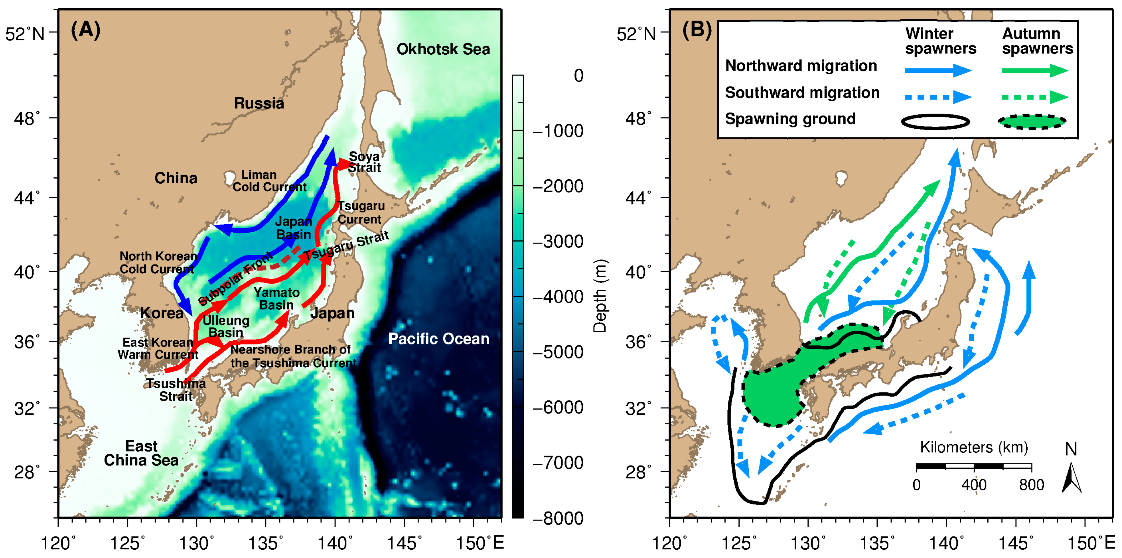
2.1. Study Area

The Sea of Japan is a semi-enclosed marginal sea in the western North Pacific with an area of roughly 1 × 10⁶ km2, geographically bounded by Japan peninsula, Sakhalin, and mainland Asia (Figure 1A). The sea is also considered as a miniature ocean because of its characteristic oceanic features, including the basin-scale gyres, mesoscale eddies, sub-polar front and thermohaline circulation [13,14]. The basin is divided by sub-polar front into cold and warm subarctic and subtropical waters, respectively [15]. The Tsushima warm current (TWC) transports warm, saline waters into the Sea of Japan through the Korea Strait. The TWC further branches out into the East Korean warm current and nearshore branch of the Tsushima current. In the north of the subarctic front, the Liman and North Korean cold currents carry cold and less salty waters southward along the coasts (Figure 1A). The notably complex physical dynamics of the Sea of Japan consequently creates a variety of habitats for the marine communities [16]. Thus, this area constitutes an important large marine ecosystem that supports commercially-valuable fishery resources, including Japanese common squid. The spawning grounds and migration routes of the seasonal cohorts of Japanese common squid in the Sea of Japan and East China Sea, as well as the western Pacific Ocean, are shown in Figure 1B (modified from [2]). The extensive seasonal migration of T. pacificus across the different ocean basins are highlighted.

2.2. Satellite-Derived Squid Occurrences

The squid fishing locations were identified from the night-time visible imageries provided and supplemented by the NOAA Defense Meteorological Satellite Program/ Operational Linescan System (DMSP/OLS) and NASA’s Visible Infrared Imager Radiometer Suite (VIIRS) onboard the newest Earth-observing satellite of the National Polar-orbiting Operational Environmental Satellite System Preparatory Project (NPP) [18]. The DMSP/OLS data were obtained from the Satellite Image Data Base (SIDaB) of Japan’s Agriculture, Forestry and Fisheries Research Information Technology Center (AFFRIT). The DMSP/OLS and NPP/VIIRS imageries were available at raw spatial resolutions of 4 km and 0.75 km, respectively. Combining the data from the sensors augmented the squid presence points for subsequent habitat modeling analyses, during the period from March to July 2012–2013, when the data availability is minimal (Table 1). The paucity of the data in spring and summer were due to the elevated temperature and corresponding increases in water vapor [2]. The detection of squid fishing locations from daily night-time satellite images from January–December, 2010–2013 was implemented using a threshold-based image classification [2]. From this two-level slicing method, the bright areas thought to be caused by the fishing fleet were extracted. It is assumed that the squid were caught in the areas where fishing vessels were located [2,3]. The earlier work by Choi et al. [3] revealed that DMSP/OLS-inferred squid fishing locations in the southwestern part of the Sea of Japan matched well with reported actual catch data and fishing vessel positions. Hence, these provide us with useful data for presence-only habitat model construction, enabling us to resolve the seasonal potential habitat patterns of T. pacificus in the Sea of Japan. Prior to the habitat model development, the detected squid fishing locations were compiled into monthly databases and gridded at 0.25° spatial resolution. This was done to match the coarsest available spatial and temporal resolutions of environmental data.

2.3. Satellite-Based Topographic and Environmental Variables

The static and environmental parameters used to infer species habitat distribution were sourced from remotely-sensed information, covering the period from January–December 2010–2013. The suite of data consisted of static habitat factor (depth) and five environmental variables (sea surface temperature (SST), chlorophyll-a (Chl-a), sea surface height anomaly (SSHA), eddy kinetic energy (EKE), zonal (u) and meridional (v) geostrophic velocity). The topographic data was from the ETOPO1 bathymetry data global relief model of Earth's surface, provided by the NOAA National Centers for Environmental Information (NCEI) [19], available at 0.01° spatial resolution. The monthly blended SST and Moderate resolution Imaging Spectroradiometer (MODIS) Chl-a data were obtained from National Oceanic and Atmospheric Administration (NOAA) data server website [20] at a source spatial footprint of 0.10°. Monthly-averaged SSHA, EKE, and geostrophic velocities were computed from the daily merged product of the mapped sea level anomaly (MSLA) and geostrophic velocities (u, v), downloaded from the Archiving Validation and Interpretation of Satellite Data (AVISO) website [21] at 0.25° spatial resolution. The EKE was then calculated from geostrophic velocities, as half of the sum of squared values of u and v [22]. Moreover, the temporal patterns of environmental, topographic, and geographical data (longitude and latitude) corresponding to squid occurrences were extracted and averaged for each month to explore their seasonal variability. All environmental and topographic data were resampled to 0.25° spatial resolution for the habitat modeling analyses.

2.4. MaxEnt Model Construction and Evaluation

The species distribution model for Japanese common squid was developed using the maximum entropy (MaxEnt) model algorithm. The MaxEnt model uses a presence-only algorithm based on a generative approach to infer species’ habitat distributions. This is achieved by combining the set of relevant environmental layers and species occurrence to identify its suitable habitat in the geographic space [23]. MaxEnt model is one of the most widely used tool for various marine habitat studies, to identify and map the key habitats of diverse marine fauna [12,24,25]. In this study, we used this model approach to resolve the seasonal potential habitat of T. pacificus in the Sea of Japan, where the potential habitat is directly proportional to the measure of habitat suitability index (HSI). The HSI ranged from 0–1, where values closer to 1 represent the preferential squid habitat.
We developed the models using MaxEnt software [26] invoked from within the BIOMOD2 package [27] in R version 3.2.5, Vienna, Austria [28]. This was done to increase the flexibility of MaxEnt software as the latter R package provides a wider suite of built-in statistical tools for evaluating the model’s predictive performance. Here, we used the spatially-matched squid fishing data (response variable) and environmental parameters (independent variables) from January–December 2010–2013. The models were designed as such, due to the short data coverage available for this study. Moreover, the likely inter-annual persistence of key frontal features in the study area could result to the stability of potential squid habitat within a four-year period. To further test for the inter-annual variability in potential squid habitat, statistical tests for homogeneity of variances were performed using Bartlett test and chi-square at alpha value (α) of 0.95 and three degrees of freedom (df). These statistical tests confirmed that the monthly variances in potential squid habitat between years were homogeneous (p > 0.05 and chi-squared > Bartlett K-squared; Table 2), suggesting no significant inter-annual variability signals were evident.
The model input was prepared using the sample with data (SWD) format as described in the online MaxEnt documentation [26]. In each monthly-compiled squid presence data, the background points were randomly selected using a 1:10 presence to pseudo-absence ratio [29] using the dismo R package [30]. These data were subsequently pooled together to generate the background SWD. The model SWD input was then apportioned to 70% training and 30% testing data sets. A total of 10 model simulations were implemented to generate the robust statistical measures of the model performance [31]. The models’ statistical performance were evaluated using threshold-independent and dependent metrics, the area under the curve (AUC) of ROC [32], true skill statistics (TSS) [33], and Cohen’s Kappa, hereafter referred to as ‘Kappa’ [34], respectively. Given these metrics, a model is considered performing when the AUC is greater than 0.5 and TSS and Kappa values are greater than 0.
Moreover, the relative contributions of each oceanographic and topographic parameters for the model simulations were computed within BIOMOD2. The procedure invokes the calculation of the correlation scores between the standard and new predictions. The standard prediction was made once the model was calibrated. Subsequently, each variable is randomized to create the new prediction. Highly correlated predictions (i.e., with slight differences in predictions) show that the randomized factor has little influence on prediction-making. The variable importance is, then, expressed as 1 minus the correlation score. The high values correspond to high variable importance and values close to 0 reveal low to no importance [27].

2.5. Spatio-Temporal Mapping of Potential Squid Habitat

For each month between 2010 and 2013, ten MaxEnt model simulations were used to generate 40 squid habitat predictions (i.e., 10 predictions per month × 4 years). Each monthly set, comprised of 40 habitat predictions, was subsequently used to compute for the pixel-wise averages and standard deviations (SD) of the suitable squid habitat (expressed in terms of HSI) from January–December. This was carried out to examine the seasonal variation of squid habitat patterns across space. These maps further highlight the regions where persistent potential squid habitat (defined as areas with low SD) were identified during the four-year period. All the mapping routines for this work were conducted using an open-source software, the generic mapping tools (GMT) version 4.5.12, Hawaii, USA [35].

3. Results

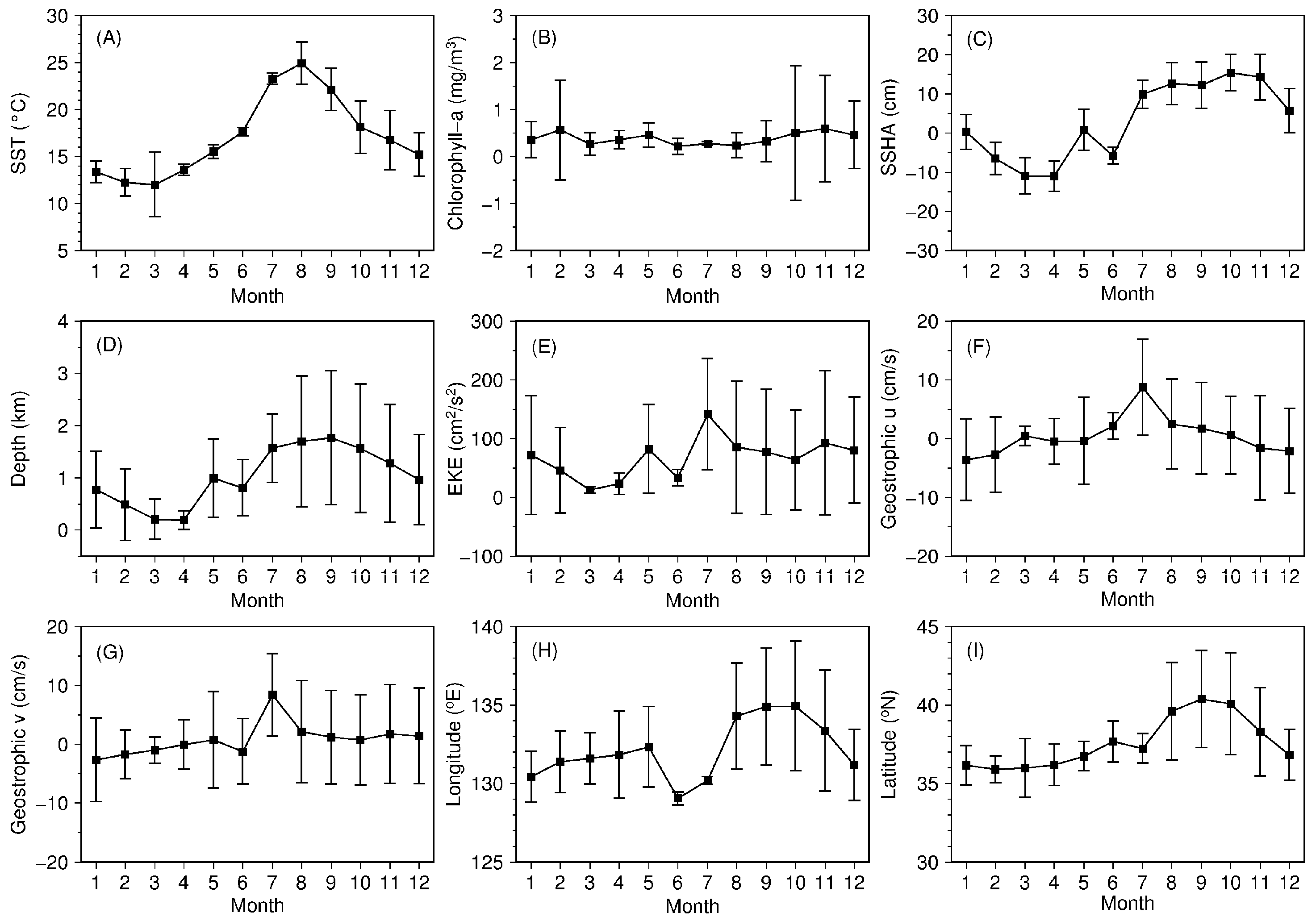
3.1. Distributional Patterns of Oceanographic and Geographic Factors in Squid Fishing Sites

The monthly mean distributions of the oceanographic and geographical variables computed in the squid fishing sites, during the four-year period are shown in Figure 2A,I. Based on these time-series, most environmental factors exhibited strong seasonality. A clear seasonal pattern is exemplified in SST distributions (Figure 2A), where low and high SSTs characterize the squid habitat from winter–spring (December–May) and summer–autumn (June–November), respectively. Highly variable SSTs were also observed during the seasonal transitions, except in spring and early summer (April–June). In contrast, Chl-a distributions (Figure 2B) showed minimal seasonality, albeit with highly variable measurements observed during autumn–winter (October–February) period. The temporal patterns of SSHA (Figure 2C) revealed a prominent shift from negative to positive SSHAs between January–June and July–December, however, the variability of measurements across months was comparable. Interestingly, similar temporal pattern was observed for the bathymetric time-series (Figure 2D), where the squid occurrences were found at shallower depths from January–June, relative to the July–December period. The EKE temporal pattern showed that squid occurrences were mostly located in regions with weaker EKEs, yet highly variable measurements were observed between months (Figure 2E).The temporal patterns for u (Figure 2F) and v (Figure 2G) components of the geostrophic velocity, however, showed similar patterns with a velocity peak in July. Moreover, the temporal patterns of geographical parameters across and along the longitudinal and latitudinal axes, revealed prominent west–east (Figure 2H) and south–north (Figure 2I) shifts of squid occurrences in winter and summer, respectively. The largest fluctuations in the zonal and meridional geographic positions across a 12-month period, were observed between August and October.

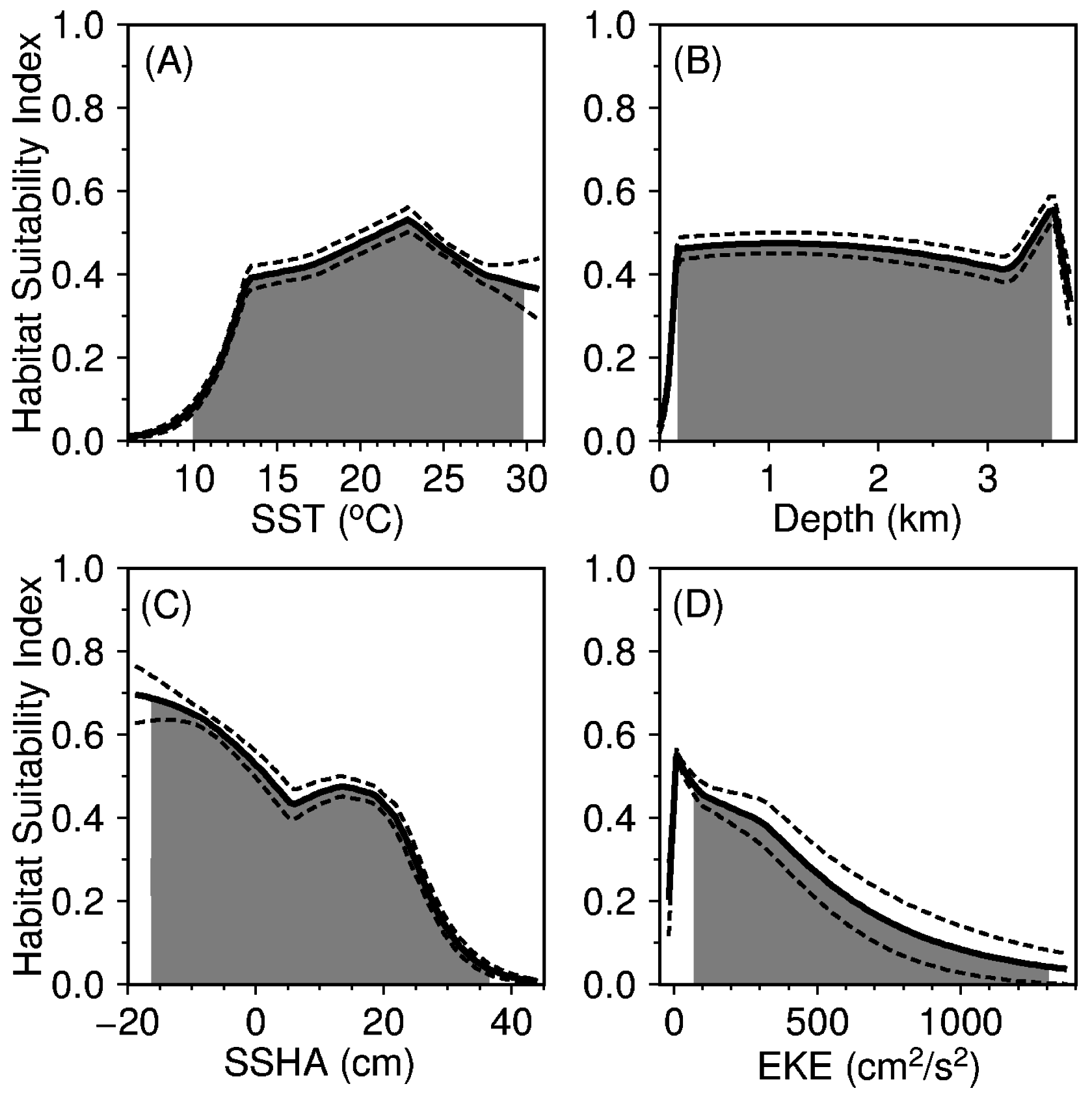
3.2. Relative Importance of Environmental Factors to Squid Habitat

The relative contributions of individual oceanographic and topographic features to the potential squid habitat (Table 3) showed that the most important variables were SST (0.81 ± 0.02), depth (0.19 ± 0.02), SSHA (0.14 ± 0.01), and EKE (0.10 ± 0.05). The rest of the oceanographic variables exhibited low (geostrophic velocity components) to almost negligible (Chl-a) effects on squid habitat predictions.
Figure 3A–D showed the generated response curves and their respective standard deviations for the four most important environmental factors. Based on these figures, the characteristic environmental ranges of the potential squid habitat between the 5th and 95th percentiles were highlighted. The percentile SST cut-off revealed that the SST range for potential squid habitat was between 10 °C –30 °C, albeit, the upper tail of the distribution exhibited the largest standard deviation at SST greater than 27 °C. The highest predicted HSI was found at 23 °C (Figure 3A). The response curve for the bathymetric factor showed that the squid potential habitat was distributed over shallow (171 m) and deeper (3580 m) areas of the basin (Figure 3B). However, a prominent peak in HSI was observed at a depth of 3600 m. For SSHA, the preferred potential squid habitat range was found between −16 and 36 cm and the highest predicted HSI was centered at cold water parcels of SSHA equal to −18 cm (Figure 3C). Moreover, the preferred squid habitat range for the EKE was between 71 and 1306 cm2/s2, with high HSI at relatively weaker EKE (Figure 3D).

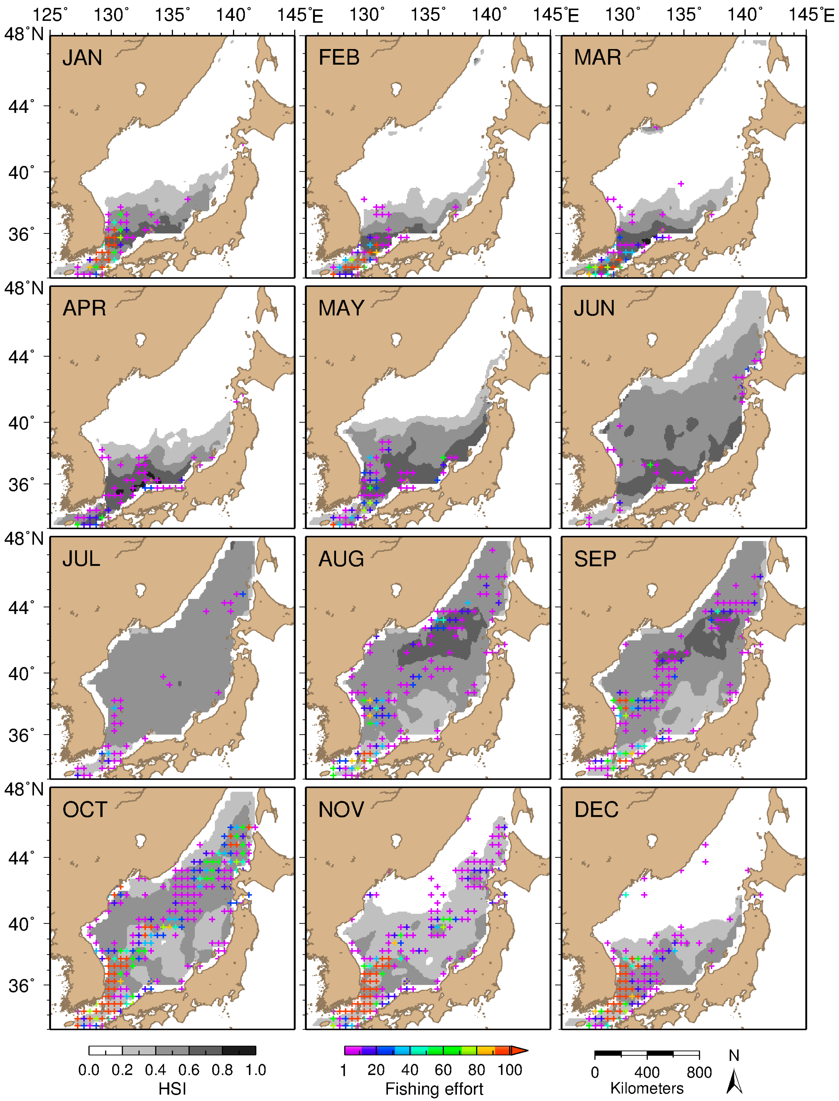
3.3. Model-Inferred Seasonal and Spatial Squid Habitat Patterns

The multiple model simulations exhibited modest and robust statistical performance based on the threshold-dependent and independent metrics (Table 4). Despite the wide distribution of squid in the basin throughout an annual cycle, the models were able to predict the squid occurrences better than when predicted in random. Based on these models, the spatio-temporal patterns of squid in the Sea of Japan showed the basin-wide differences in predicted habitat distributions over an inter-seasonal time-scale.
The monthly-averaged habitat predictions overlain with the corresponding distribution of the fishing effort from January to December are shown in Figure 4. During the winter-spring period (December–May), the squid potential habitat was largely confined within a narrow area in the southern tip of the basin (125°–140°E and 33°–41°N). The predicted suitable habitat was also found to correspond well with the spatial distributions of the squid fishing activities. The smallest habitat areal extents during this period were mainly observed from February to March, covering the waters off the Tsushima Strait and nearshore areas of South Korea and Japan. The onset of summer (June) marked the basin-wide expansion of potential squid habitat, albeit the patches of highly-suitable habitat were found along the nearshore waters of Japan. In July, the potential habitat distribution throughout the basin revealed a uniform pattern, with squid fishing activities gradually extending off the central and northern parts of the basin. However, distinct patches of highly-suitable habitat were recognizable from August–November. This pattern is accompanied with the extensive fishing activities along the entire stretch of the basin. Between August and September, large patches of highly suitable habitat were formed in Japan basin (40°–44°N and 132°–140°E). These regions also exhibited moderate level of fishing activities. In October and November, the squid fishing activities were most intensified and were located off the highly suitable habitat regions in the central part of the Sea of Japan. While the offshore fishing activities persisted through November, potential squid habitat exhibited considerable areal reduction with formation of highly suitable zones off the nearshore waters of Japan and Korea. Throughout the year, however, the highest squid fishing activities were consistently located off the shallow waters around the Tsushima Strait.

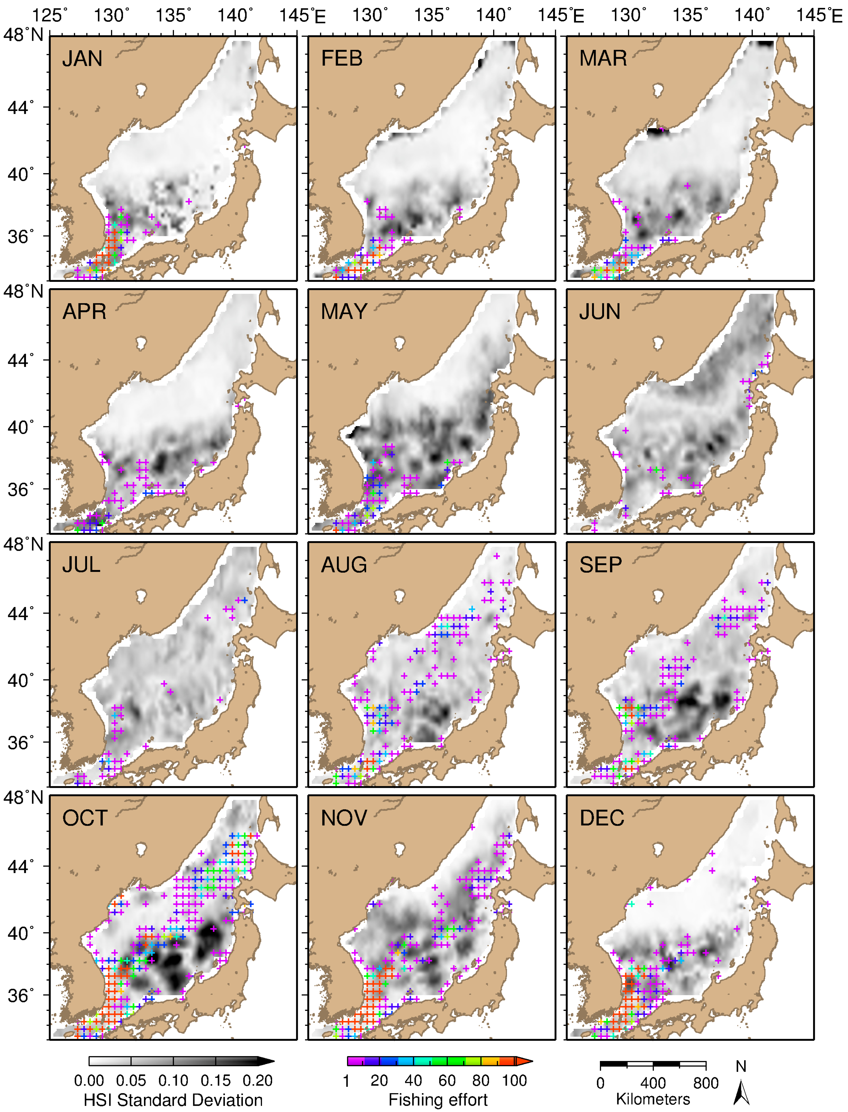
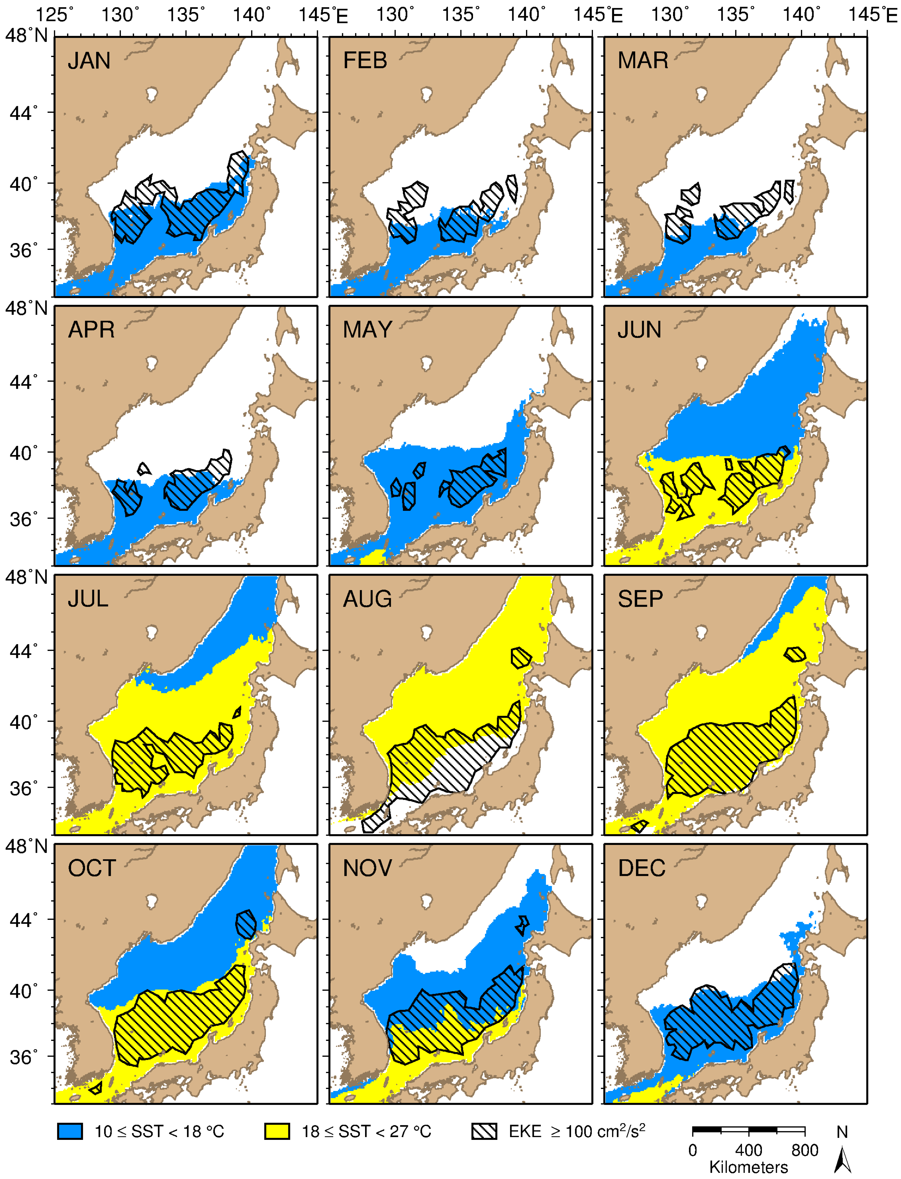
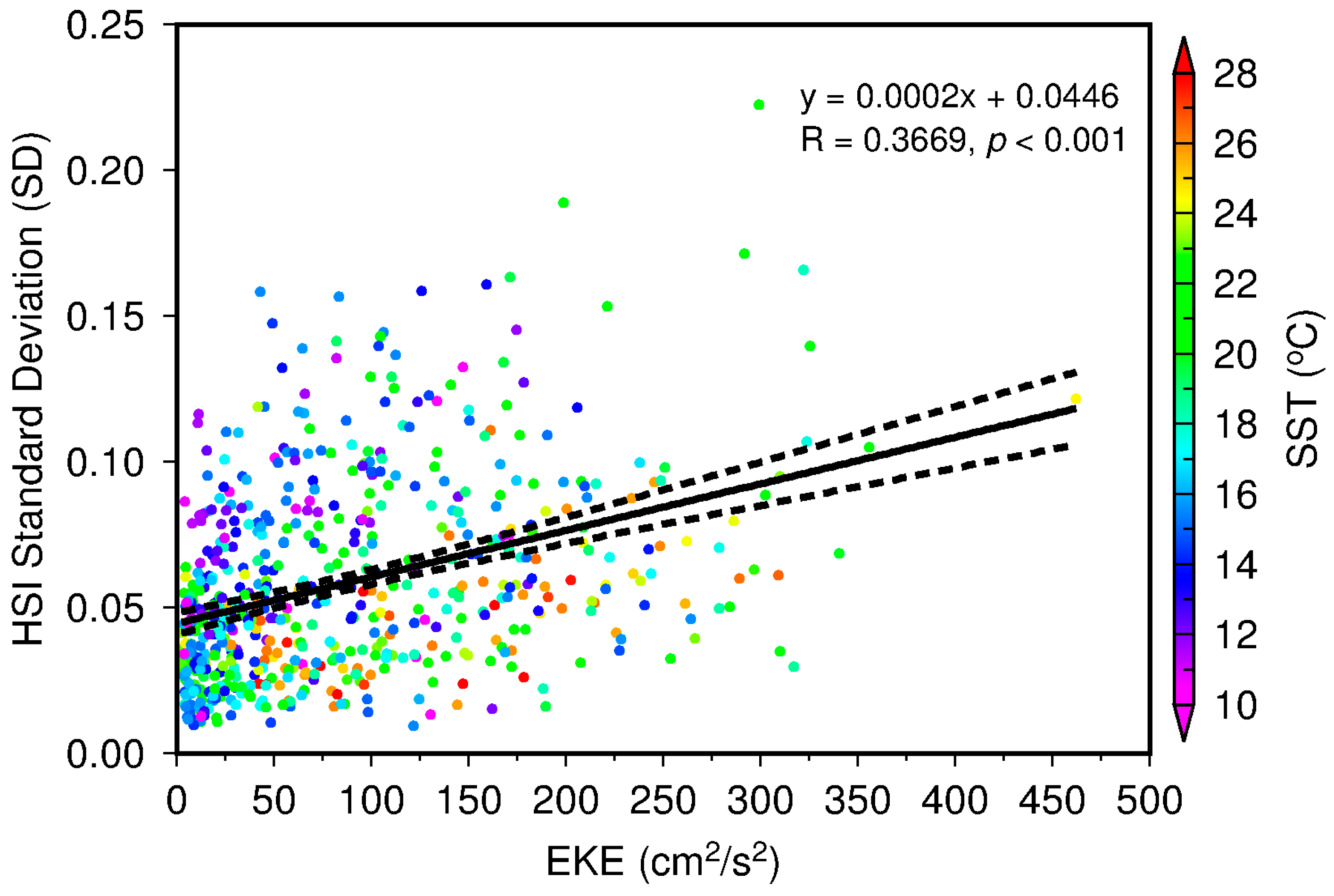
3.4. Stability of Potential Squid Habitat and Patterns of Key Oceanographic Conditions

The pixel-wise standard deviation (SD) of the potential squid habitat from January–December are shown in Figure 5. Based on this figure, the stable suitable areas for squid off the Tsushima Strait (i.e., with lower SD) corresponded to the regions where intensive fishing activities occurred. In the winter–spring period (December–May), relatively variable suitable habitat zones were located off the Ulleung and Yamato basins. In summer (June–August), the unstable potential habitat patches decreased off these basins and significantly increased in autumn (September–November). In October, highly unstable potential habitat patches were predominantly observed off the Yamato basin.
The spatial patterns of oceanographic conditions based on SST and EKE are shown in Figure 6. From these maps, the contraction and expansion of favorable SST range (10 °C–27 °C) for squid habitat were captured and resembled the spatial distributions of the predicted HSI (Figure 4). During the winter–spring period (December–March), the favorable SST distributions were comprised of colder waters (10 °C–18 °C). This is further accompanied with the relatively smaller patches of moderate–high EKE, located off the Ulleung and Yamato basins. In summer (June–August), the preferred SST limit gradually transitioned to the dominance of the warm SST bin (18 °C–27 °C) and persisted through mid-autumn (October). This warm water pattern regressed to the cold water phase by the end of the autumn season (November). These periods are marked by the expansion of moderate–high EKE zone, extending towards the Tsushima Strait. Between October and November, the colder waters encroached further south, consequently limiting the spatial distribution of warm waters. Despite the SST shift observed for these months, the areal extent of moderate–high EKE zones in the northern part of the Tsushima Strait remained significant. Moreover, a significant positive correlation between the instability of the potential squid habitat and mesoscale activity is further highlighted in Figure 7. More stable suitable squid habitat was also located at warmer SSTs, with low–moderate EKE.

4. Discussion

The present study has taken advantage of available datasets from multi-sensor satellite platforms to explore the seasonal distributions of squid resources in the Sea of Japan. It further emphasized the use of combined data from recently-launched satellite sensors (NPP/VIIRS) and DMSP/OLS for the detection of squid fishing vessels in the basin. These in turn, provided potential occurrence data sources for developing species distribution models for T. pacificus. In the ocean, collection of fishery-independent data through biological surveys remains a challenge [36]. Therefore, tapping alternative data sources to further fisheries studies has attracted fisheries scientists and managers. The night-time visible imageries have been earlier used in a variety of marine applications, including that for tracking ship and fishing activities [2,3,37,38]. Our study further expanded the practical applications of these data to examine the squid-environment interactions through a habitat modeling approach.
The species distribution models are widely used tools to examine the habitat preferences of species, map its potential geographical distributions and explore species-environment interactions [39]. Here, we developed the species distribution models for Japanese common squid to examine the seasonal habitat patterns in response to relevant oceanographic and topographic factors. To our knowledge, this is the first satellite–based habitat modeling study for T. pacificus in the Sea of Japan. From our results, the MaxEnt-derived habitat models have shown modest statistical performance in predicting squid habitat (Table 4). Moreover, averaging the monthly squid habitat predictions from multiple model simulations generated robust spatial squid habitat maps (Figure 4). From these maps, the spatial changes in potential squid habitat distributions within an inter-seasonal timescale were evident. The salient zonal and meridional shifts of preferential squid habitat from winter–spring to summer–autumn periods are potentially driven by the responses of squid to environmental changes and physiological processes that are associated with its annual life cycle. The model-inferred environmental ranges of the suitable habitat highlighted the favorable oceanographic conditions for squid (Figure 3). These conditions were largely regulated by the seasonal distribution patterns of SST and proxies for mesoscale activity (SSHA and EKE). These oceanographic factors have been shown to exert significant impacts on habitat distributions and abundance of pelagic species likely through local nutrient enhancement [25,40].
Previous field and experimental studies have shown that temperature is crucial for the growth and survival of T. Pacificus. Off the southern part of the Sea of Japan, extending towards the East China Sea in winter, SST values in this area ranged from 12.7 °C –23.2 °C. Within this observed SST range, SST from 15 °C–18 °C were found favorable for spawning [41]. Moreover, results from laboratory studies of reared individuals showed that normal embryonic development occurred in temperatures between 14 °C and 26 °C, with the highest survival rates from 14.7 °C and 22.2 °C [42,43]. Model-derived SST ranges inferred from our study (Figure 3A) were comparable with these reported values, albeit our results covered a broader SST limit than the latter. This could possibly suggest that T. pacificus are likely to inhabit region with wider temperature limits in the wild and, hence, encounter remarkably dynamic oceanographic conditions throughout its short life span. Other ommastrephids, such as jumbo squid (Dosidicus gigas), for instance, were reported to exhibit irregular seasonal invasions in areas past their normal environmental ranges. Such events were attributed to their active feeding migrations during years of high abundance [44].
Mesoscale activity in the ocean has also been an important physical driver of species distribution and abundance. In the western North Pacific Ocean, meanders and eddies spinning off from the strong boundary current were known to create favorable feeding environments for economically-important fisheries [12,45]. In the Sea of Japan, similar gyral features were also identified from previous studies [46,47]. In the present work, moderate–strong eddy activities (Figure 6) were situated in the southern part of the basin (north of the Tsushima Strait) from July–December, which also corresponded to the zones with significant fishing activity and high predicted squid habitat (Figure 4). While the enhanced eddy activity appeared to support elevated biological production [48], the variability in spatial distribution of the oceanographic features over time could also affect the persistence of the potential squid habitat on the seasonal and inter-annual periods. A similar scenario was shown in our results, highlighting the unstable potential habitat zones (i.e., highest HSI SD; Figure 5), located off the eddy-rich regions. This is further reinforced by the significant positive correlation (Figure 7) between the standard deviation of HSI and EKE, extracted from the squid fishing locations from January–December. The warmer SST attribute of highly stable potential habitat could further suggest its association with the warm-water eddies, which are prominent circulation features in the Sea of Japan [2,3].
In contrast, static factors such as bathymetry, which was also recognized as the second most important variable in this study, showed that the squid used a whole range of topographic habitat from shallow to deeper areas from January–December (Figure 3). The pattern of utilization could be potentially linked to the preferences of the squid in searching for the optimal spawning and foraging grounds. Following the reproduction hypothesis for T. pacificus, adult squid generally moved to the shallow continental shelves and slopes (100–500 m) for spawning [1,43]. However, during summer feeding migration (June–August), the squid undergoes a northward movement into deeper waters of the Sea of Japan. The southward spawning migration of the squid subsequently ensues from September–November, traversing along the deep water corridors of the basin [2]. This is also accompanied with the seasonal cooling of the north and central parts of the Sea of Japan (Figure 6), as the sub-polar front intensifies and pushes the frontal boundary further south. Interestingly, the formation of distinct highly suitable habitat patches in the northeastern part of Japan basin from August–September (Figure 4) is coincident with the presence of an isolated frontal zone trapped by a seamount around this area [49].

5. Conclusions

The habitat models developed for the T. Pacificus using all-satellite-based information in the Sea of Japan, underscored the enormous potential of remotely-sensed data for understanding the spatial and temporal squid habitat patterns, emerging from the species-environment interaction. The use of fishing vessel positions detected from night-time visible images provided an alternative data source for exploring the preferential squid habitat distributions. The use of the NPP/VIIRS data, which have an improved ability than DMSP/OLS to accurately detect the fishing fleets, has significantly augmented the samples for constructing the presence-only models. However, we also recognized that the data could similarly suffer from sampling biases and false positive detection of squid occurrences. Hence, future studies complementing the satellite-detected squid presence with actual fishery information, when available, could improve the predictive performance of the statistical models. Longer temporal coverage of response data for habitat modeling analyses could also assist in making robust detection of potential habitat hotspots and exploring the inter-annual variability in distributions of predicted squid habitat. Despite the inherent data limitation, our habitat modeling analyses have shown modest predictive performance. In the process, our analyses were able to reveal pertinent insights on squid habitat responses to seasonal changes in oceanographic conditions and reinforced the findings of observational and experimental studies. Our results also underpinned the roles of oceanographic features and their respective attributes in regulating the persistence/stability of squid habitat. These information could be invaluable in marine spatial planning and management of squid resources in the Sea of Japan.

Acknowledgments

The authors acknowledge Japan’s Agriculture, Forestry and Fisheries Research Information Technology Center (AFFRIT) for providing the DMSP/OLS data and the NOAA data centers for NPP/VIIRS images. We thank the 3 anonymous reviewers for their constructive comments and suggestions that significantly improve the content and presentation of this manuscript. We are also grateful to Fumihiro Takahashi for his technical assistance in the download and processing of NPP/VIIRS DNB data. We are extending our thanks to Puneeta Pandey and Xun Zhang for helpful discussions on squid biology and applications of DMSP/OLS data. We also thank Ryan Matthew A. Mendoza for the encouragement in the course of writing the manuscript.

Author Contributions

I.D.A., M.D. and S.-I. S. conceived the idea for this study; M.D. processed and prepared the night-time visible images; I.D.A. conducted the habitat modeling simulations and analyzed the data; S.-I.S. and T.H. contributed materials/analysis tools; I.D.A. wrote the paper with input from all of the authors. All of the authors reviewed and approved the submitted manuscript.

Conflicts of Interest

The authors declare no conflict of interest.

References

  1. Sakurai, Y.; Kiyofuji, H.; Saitoh, S.; Goto, T.; Hiyama, Y. Changes in inferred spawning areas of Todarodes pacificus (Cephalopoda: Ommastrephidae) due to changing environmental conditions. ICES J. Mar. Sci. 2000, 57, 24–30. [Google Scholar] [CrossRef]
  2. Kiyofuji, H.; Saitoh, S.-I. Use of nighttime visible images to detect Japanese common squid Todarodes pacificus fishing areas and potential migration routes in the sea of Japan. Mar. Ecol. Prog. Ser. 2004, 276, 173–186. [Google Scholar] [CrossRef]
  3. Choi, K.; Lee, C.I.; Hwang, K.; Kim, S.-W.; Park, J.-H.; Gong, Y. Distribution and migration of Japanese common squid, Todarodes pacificus, in the southwestern part of the east (Japan) sea. Fish. Res. 2008, 91, 281–290. [Google Scholar] [CrossRef]
  4. Chen, X.; Liu, B.; Chen, Y. A review of the development of Chinese distant-water squid jigging fisheries. Fish. Res. 2008, 89, 211–221. [Google Scholar] [CrossRef]
  5. Food and Agriculture Organization. Myopsid and oegopsid squids. In Cephalopods of the World: An Annotated and Illustrated Catalogue of Cephalopod Species Known to Date; Jereb, P., Roper, C.F.E., Eds.; FAO United Nations: Rome, Italy, 2010; Volume 2, pp. 1–605. [Google Scholar]
  6. Food and Agriculture Organization. Fishery and aquaculture statistics 2012. In FAO Yearbook; FAO United Nations: Rome, Italy, 2014. [Google Scholar]
  7. Tamura, T.; Fujise, Y. Geographical and seasonal changes of the prey species of minke whale in the northwestern Pacific. ICES J. Mar. Sci. 2002, 59, 516–528. [Google Scholar] [CrossRef]
  8. Okutani, T. Todarodes pacificus. In Cephalopod Life Cycles; Boyle, P.R., Ed.; Academic Press: London, UK, 1983; pp. 201–214. [Google Scholar]
  9. Kang, Y.S.; Kim, J.Y.; Kim, H.G.; Park, J.H. Long-term changes in zooplankton and its relationship with squid, Todarodes pacificus, catch in Japan/East Sea. Fish. Oceanogr. 2002, 11, 337–346. [Google Scholar] [CrossRef]
  10. Phillips, S.J.; Dudik, M.; Schapire, R.E. A maximum entropy approach to species distribution modeling. In Proceedings of the Twenty-First International Conference on Machine Learning, Banff, AB, Canada, 4–8 July 2004; p. 83.
  11. Lefkaditou, E.; Politou, C.-Y.; Palialexis, A.; Dokos, J.; Cosmopoulos, P.; Valavanis, V. Influences of environmental variability on the population structure and distribution patterns of the short-fin squid Illex coindetii (Cephalopoda: Ommastrephidae) in the Eastern Ionian Sea. Hydrobiologia 2008, 612, 71–90. [Google Scholar] [CrossRef]
  12. Alabia, I.D.; Saitoh, S.-I.; Mugo, R.; Igarashi, H.; Ishikawa, Y.; Usui, N.; Kamachi, M.; Awaji, T.; Seito, M. Seasonal potential fishing ground prediction of neon flying squid (Ommastrephes bartramii) in the western and central North Pacific. Fish. Oceanogr. 2015, 24, 190–203. [Google Scholar] [CrossRef]
  13. Chang, K.-I.; Ito, S.-I.; Mooers, C.N.K.; Yoon, J.-H. Observation and modeling of the ocean circulation and marine ecosystem for creams/pices. J. Mar. Syst. 2009, 78, 195–199. [Google Scholar] [CrossRef]
  14. Jo, C.O.; Park, S.; Kim, Y.H.; Park, K.-A.; Park, J.J.; Park, M.-K.; Li, S.; Kim, J.-Y.; Park, J.-E.; Kim, J.-Y.; et al. Spatial distribution of seasonality of seaWiFS chlorophyll-a concentrations in the East/Japan Sea. J. Mar. Syst. 2014, 139, 288–298. [Google Scholar] [CrossRef]
  15. Ashjian, C.; Arnone, R.; Davis, C.; Jones, B.; Kahru, M.; Lee, C.; Mitchell, B.G. Biological structure and seasonality in the Japan/east sea. Oceanography 2006, 19, 122–133. [Google Scholar] [CrossRef]
  16. Kim, S.; Zhang, C.-I. Fish and fisheries. In Oceanography of the East Sea (Japan Sa); Chang, K.-I., Zhang, C.-I., Park, C., Kang, D.-J., Ju, S.-J., Lee, S.-H., Wimbush, M., Eds.; Springer International Publishing: Cham, Switzerland, 2016; pp. 327–345. [Google Scholar]
  17. Yoshikawa, Y.; Awaji, T.; Akitomo, K. Formation and circulation processes of intermediate water in the Japan sea. J. Phys. Oceanogr. 1999, 29, 1701–1722. [Google Scholar] [CrossRef]
  18. National Oceanic and Atomspheric Administration. Comprehensive Large Array-data Stewardship System (CLASS) Data Description. Available online: http://www.nsof.class.noaa.gov/saa/products/search?datatype_family=VIIRS_SDR (accessed on 9 November 2015).
  19. ETOPO1 Global Relief Model. Available online: http://ngdc.noaa.gov/mgg/global/ (accessed on 27 April 2016).
  20. National Oceanic and Atomspheric Administration ERDDAP. Available online: http://coastwatch.pfeg.noaa.gov/erddap/index.html (accessed on 20 April 2016).
  21. AVISO Satellite Altimetry Data. Available online: http://www.aviso.altimetry.fr/en/home.html (accessed on 23 April 2016).
  22. Chavanne, C.P.; Klein, P. Can oceanic submesoscale processes be observed with satellite altimetry? Geophys. Res. Lett. 2010, 37, L22602. [Google Scholar] [CrossRef]
  23. Phillips, S.J.; Anderson, R.P.; Schapire, R.E. Maximum entropy modeling of species geographic distributions. Ecol. Model. 2006, 190, 231–259. [Google Scholar] [CrossRef]
  24. McClellan, C.M.; Brereton, T.; Dell'Amico, F.; Johns, D.G.; Cucknell, A.-C.; Patrick, S.C.; Penrose, R.; Ridoux, V.; Solandt, J.-L.; Stephan, E.; et al. Understanding the distribution of marine megafauna in the english channel region: Identifying key habitats for conservation within the busiest seaway on earth. PLoS ONE 2014, 9, e89720. [Google Scholar] [CrossRef] [Green Version]
  25. Alabia, I.D.; Saitoh, S.-I.; Mugo, R.; Igarashi, H.; Ishikawa, Y.; Usui, N.; Kamachi, M.; Awaji, T.; Seito, M. Identifying pelagic habitat hotspots of neon flying squid in the temperate waters of the central North Pacific. PLoS ONE 2015, 10, e0142885. [Google Scholar] [CrossRef] [Green Version]
  26. Maxent Software for Species Habitat Modeling. Available online: https://www.cs.princeton.edu/~schapire/maxent/ (accessed on 6 May 2016).
  27. Thuiller, W.; Georges, D.; Robin, E. Biomod2: Ensemble Platform for Species Distribution Modeling. Available online: http://CRAN.R-project.org/package=biomod2 (accessed on 31 August 2014).
  28. R Core Team. R: A Language and Environment for Statistical Computing; R Foundation for Statistical Computing: Vienna, Austria, 2015. [Google Scholar]
  29. Barbet-Massin, M.; Jiguet, F.; Albert, C.H.; Thuiller, W. Selecting pseudo-absences for species distribution models: How, where and how many? Methods Ecol. Evol. 2012, 3, 327–338. [Google Scholar] [CrossRef]
  30. Hijmans, R.J.; Phillips, S.J.; Leathwick, J.R.; Elith, J. Dismo: Species distribution modeling. Available online: https://cran.R-project.Org/package=dismo (accessed on 31 August 2014).
  31. Hijmans, R.J. Cross-validation of species distribution models: Removing spatial sorting bias and calibration with a null model. Ecology 2012, 93, 679–688. [Google Scholar] [CrossRef]
  32. Swets, J.A. Measuring the accuracy of diagnostic systems. Science 1988, 240, 1285–1293. [Google Scholar] [CrossRef]
  33. Allouche, O.; Tsoar, A.; Kadmon, R. Assessing the accuracy of species distribution models: Prevalence, kappa and the true skill statistic (TSS). J. Appl. Ecol. 2006, 43, 1223–1232. [Google Scholar] [CrossRef]
  34. Cohen, J. A coefficient of agreement for nominal scales. Educ. Psychol. Meas. 1960, 20, 37–46. [Google Scholar] [CrossRef]
  35. Wessel, P.; Smith, W.H.F.; Scharroo, R.; Luis, J.; Wobbe, F. Generic mapping tools: Improved version released. Eos Trans. Am. Geophys. Union 2013, 94, 409–410. [Google Scholar] [CrossRef]
  36. Dell, J.; Wilcox, C.; Hobday, A.J. Estimation of yellowfin tuna (Thunnus albacares) habitat in waters adjacent to Australia’s east coast: Making the most of commercial catch data. Fish. Oceanogr. 2011, 20, 383–396. [Google Scholar] [CrossRef]
  37. Straka, W.; Seaman, C.; Baugh, K.; Cole, K.; Stevens, E.; Miller, S. Utilization of the Suomi national polar-orbiting partnership (NPP) visible infrared imaging radiometer suite (VIIRS) day/night band for arctic ship tracking and fisheries management. Remote Sens. 2015, 7, 971–989. [Google Scholar] [CrossRef]
  38. Syah, A.F.; Saitoh, S.-I.; Alabia, I.D.; Hirawake, T. Predicting potential fishing zones for Pacific saury (Cololabis saira) with maximum entropy models and remotely sensed data. Fish. Bull. 2016, 114, 330–343. [Google Scholar] [CrossRef]
  39. Elith, J.; Leathwick, J.R. Species distribution models: Ecological explanation and prediction across space and time. Annu. Rev. Ecol. Evol. Syst. 2009, 40, 677–697. [Google Scholar] [CrossRef]
  40. Mugo, R.M.; Saitoh, S.-I.; Takahashi, F.; Nihira, A.; Kuroyama, T. Evaluating the role of fronts in habitat overlaps between cold and warm water species in the western North Pacific: A proof of concept. Deep Sea Res. Part II Top. Stud. Oceanogr. 2014, 107, 29–39. [Google Scholar] [CrossRef]
  41. Kidokoro, H.; Sakurai, Y. Effect of water temperature on gonadal development and emaciation of Japanese common squid Todarodes pacificus (Ommastrephidae). Fish. Sci. 2008, 74, 553–561. [Google Scholar] [CrossRef]
  42. Yamamoto, J.; Miyanaga, S.; Fukui, S.; Sakurai, Y. Effect of temperature on swimming behavior of paralarvae of the Japanese common squid Todarodes pacificus. Bull. Japanese Soc. Fish. Oceanogr. 2012, 76, 18–23. [Google Scholar]
  43. Puneeta, P.; Vijai, D.; Yoo, H.-K.; Matsui, H.; Sakurai, Y. Observations on the spawning behavior, egg masses and paralarval development of the ommastrephid squid Todarodes pacificus in a laboratory mesocosm. J. Exp. Biol. 2015, 218, 3825–3835. [Google Scholar] [CrossRef]
  44. Nigmatullin, C.M.; Nesis, K.N.; Arkhipkin, A.I. A review of the biology of the jumbo squid Dosidicus gigas (Cephalopoda: Ommastrephidae). Fish. Res. 2001, 54, 9–19. [Google Scholar] [CrossRef]
  45. Zainuddin, M.; Kiyofuji, H.; Saitoh, K.; Saitoh, S.-I. Using multi-sensor satellite remote sensing and catch data to detect ocean hot spots for albacore (Thunnus alalunga) in the northwestern North Pacific. Deep Sea Res. Part II Top. Stud. Oceanogr. 2006, 53, 419–431. [Google Scholar] [CrossRef]
  46. Morimoto, A.; Yanagi, T.; Kaneko, A. Eddy field in the Japan sea derived from satellite altimetric data. J. Oceanogr. 2000, 56, 449–462. [Google Scholar] [CrossRef]
  47. Lee, D.-K.; Niiler, P. Eddies in the southwestern East/Japan Sea. Deep Sea Res. Part I Oceanogr. Res. Pap. 2010, 57, 1233–1242. [Google Scholar] [CrossRef]
  48. Gaube, P.; Chelton, D.B.; Strutton, P.G.; Behrenfeld, M.J. Satellite observations of chlorophyll, phytoplankton biomass, and ekman pumping in nonlinear mesoscale eddies. J. Geophys. Res Oceans 2013, 118, 6349–6370. [Google Scholar] [CrossRef]
  49. Park, K.-A.; Chung, J.Y.; Kim, K. Sea surface temperature fronts in the East (Japan) sea and temporal variations. Geophys. Res. Lett. 2004, 31, L07304. [Google Scholar] [CrossRef]
Figure 1. (A) Map of the Sea of Japan describing the major topographic and oceanographic features in the study area [17]. Major current systems are color-coded based on their temperature characteristic as either warm (red) or cold (blue) currents and the subpolar front is shown in broken line; (B) Map showing the spawning and migration routes of seasonal cohorts of Japanese common squid in the Sea of Japan, East China Sea, and western Pacific Ocean [2].
Remotesensing 08 00921 g001
Figure 2. Monthly time-series of the (A) SST; (B) Chl-a; (C) SSHA; (D) Depth; (E) EKE; (F) geostrophic u; (G) geostrophic v; (H) longitude; and (I) latitude at the squid fishing locations from January–December, 2010–2013. Vertical bars correspond to the ±1 standard deviation.
Remotesensing 08 00921 g002
Figure 3. Response curves of the most highly influential environmental factors: (A) SST; (B) depth; (C) SSHA; and (D) EKE, averaged from 10 MaxEnt model simulations. Broken lines correspond to ±1 standard deviation and shaded regions correspond to the area within the 5th and 95th percentiles.
Remotesensing 08 00921 g003
Figure 4. Monthly-averaged potential squid habitat in the Sea of Japan from multiple model simulations developed from January–December, 2010–2013. Overlain are the monthly gridded fishing efforts derived from night-time satellite images.
Remotesensing 08 00921 g004
Figure 5. Monthly-averaged standard deviation of potential squid habitat in the Sea of Japan from multiple model simulations developed from January–December, 2010–2013. Overlain are the monthly gridded fishing efforts derived from night-time satellite images.
Remotesensing 08 00921 g005
Figure 6. Monthly maps of favorable SST (10 °C–27 °C) characterizing the squid habitat from January–December, 2010–2013. The SST range was divided into the colder (blue) and warmer (yellow) bins. The black polygons correspond to areas with moderate to high EKE values.
Remotesensing 08 00921 g006
Figure 7. Scatterplot of EKE and HSI standard deviations (SD) extracted from squid fishing locations, from January–December. All data points were plotted in circles and color-scaled with SST (n = 602). The black solid line corresponds to the linear fit and the dotted lines are confidence bounds for the fitted coefficients at a 95% confidence interval.
Remotesensing 08 00921 g007
Table 1. Monthly-compiled squid fishing points detected from the daily DMSP/OLS night-time visible images from January–December, 2010–2013. The values in parenthesis are the augmented squid fishing locations from the DMSP/OLS and NPP/VIIRS imageries.
Year/Month2010201120122013
January12110036342908
February1794792171133
March0413131 (3198)171 (2861)
April1594156 (2539)0 (1541)
May1792914 (14)205 (2948)
June0210 (714)8 (8)
July06101 (382)40 (765)
August978471505371
September3682167319562250
October2881320853873158
November3300281415224722
December3127396323741044
Table 2. Summary statistics showing the results of Bartlett’s test and chi-square (α = 0.95; df = 3) to test for the homogeneity in variances in the potential squid habitat for each month within the four-year period (2010–2013).
MonthBartlett K-Squaredp-Valuechi-Squared
January0.57310.90267.8147
February0.45500.79657.8147
March4.21200.23957.8147
April4.54260.20857.8147
May3.41460.33207.8147
June0.53150.91197.8147
July2.55500.46547.8147
August0.70820.87137.8147
September0.34330.95177.8147
October0.56410.75427.8147
November0.65130.88467.8147
December0.49900.91917.8147
Table 3. Relative contribution of environmental variables averaged across all model simulations. The mean and standard deviation values of environmental factors with highest model contributions are highlighted in bold. The u and v correspond to geostrophic velocity components along the zonal and meridional planes, respectively.
StatisticsEnvironmental Variables
SSTChl-aSSHAEKEuvdep
Mean 0.8080.0040.1410.0990.0400.0230.186
Standard Deviation0.0230.0070.0120.0480.0230.0130.015
Table 4. Summary statistics of model performance from multiple habitat model simulations using the BIOMOD2 package in R. The statistical metrics were comprised of threshold-independent (AUC and TSS) and –dependent (Kappa) performance measures.
StatisticsModel Performance Metrics
AUC TSS Kappa
Mean0.6950.3060.132
Standard Deviation0.0100.0100.010

