Statistical Correlation between Monthly Electric Power Consumption and VIIRS Nighttime Light

Abstract

The nighttime light (NTL) imagery acquired from the Visible Infrared Imaging Radiometer Suite (VIIRS) Day/Night Band (DNB) enables feasibility of investigating socioeconomic activities at monthly scale, compared with annual study using nighttime light data acquired from the Defense Meteorological Satellite Program/Operational Linescan System (DMSP/OLS). This paper is the first attempt to discuss the quantitative correlation between monthly composite VIIRS DNB NTL data and monthly statistical data of electric power consumption (EPC), using 14 provinces of southern China as study area. Two types of regressions (linear regression and polynomial regression) and nine kinds of NTL with different treatments are employed and compared in experiments. The study demonstrates that: (1) polynomial regressions acquire higher reliability, whose average R square is 0.8816, compared with linear regressions, whose average R square is 0.8727; (2) regressions between denoised NTL with threshold of 0.3 nW/(cm²·sr) and EPC steadily exhibit the strongest reliability among the nine kinds of processed NTL data. In addition, the polynomial regressions for 12 months between denoised NTL with threshold of 0.3 nW/(cm²·sr) and EPC are constructed, whose average values of R square and mean absolute relative error are 0.8906 and 16.02%, respectively. These established optimal regression equations can be used to accurately estimate monthly EPC of each province, produce thematic maps of EPC, and analyze their spatial distribution characteristics.

1. Introduction

In recent years, the technology and application of remote sensing of nighttime light have attracted increasingly extensive attention [1,2,3,4,5,6,7,8,9,10,11,12,13,14]. Nighttime light (NTL) imagery acquired by remote sensing technology intuitively exhibit the distributions of artificial nocturnal radiances, which is an increasingly useful indicator in investigating socioeconomic activities of human being [4,5,6,7,8,9,10,11,12,13,14].

Numerous studies have demonstrated that the range and intensity of NTL are closely correlated to gross regional products (GRP) [6,15,16,17], size and density of population [17,18,19], urbanization [2,20,21], electricity consumption [1,6,22,23,24], light pollution [25,26,27], carbon dioxide (CO₂) emissions [28,29], and humanitarian disasters, etc. [30,31].

Electric power consumption (EPC) is a basic index in measuring regional energy consumption, which can not only objectively reflect economic performance situation, but also exhibit industrial structure change and energy consumption level. Obtaining accurate and timely EPC is of great practical significance in optimizing allocation of power resources and monitoring economic performance situation.

Two kinds of remotely sensed NTL data, the Defense Meteorological Satellite Program/Operational Linescan System (DMSP/OLS) and the Visible Infrared Imaging Radiometer Suite Day/Night Band (VIIRS DNB) onboard the Suomi National Polar Partnership (SNPP) satellite, were often used for remote sensing-based estimation of EPC [3,5,6].

DMSP/OLS data has been widely used due to its long temporal coverage, from 1992 to 2013, which was convenient for social and economic research of long time series [18,23]. Compared with DMSP/OLS data, the VIIRS DNB data was superior with higher spatial resolution (15 arc-second vs. 30 arc-second of DMSP/OLS), shorter temporal intervals (monthly vs. annual of DMSP/OLS) and wider radiometric detection range (free from saturation problem), which usually produced more reliable research results [5,6].

Elvidge et al. demonstrated the high correlation between DMSP/OLS NTL and EPC for 21 countries [1]. Chand et al. investigated spatial and temporal variations of EPC in India during 1993 to 2002 using DMSP/OLS [32]. He et al. built models in estimating EPC in Mainland China using saturation-corrected DMSP/OLS NTL data with high average R up to 0.93 [33]. Xie et al. investigated the influences of affluence, urbanization, technology, temperature, and NTL pattern on relationship between EPC and DMSP/OLS NTL data and suggested that EPC increased with higher per capita GDP, urbanization rate, high-technology exports, and lower agricultural development, and generally reduced with higher temperature and more agglomerate human activities [34]. Shi et al. evaluated and compared the spatiotemporal patterns of urban electricity consumption within different spatial boundaries, including the city administrative area, city district, urban center, and urban built-up area [22].

Shi et al. compared linear regressions between EPC and 2 kinds of NTL data (DMSP/OLS and VIIRS DNB) and proved that higher R² value was obtained by using VIIRS DNB data for linear regression [6]. Falchetta et al. demonstrated the effectiveness of interannual variation of VIIRS DNB NTL data in predicting within-country changes of power consumption in lower-middle income countries [35].

Previous studies have focused mainly on the quantitative relationship between NTL data and statistical variables over relatively long-time scales (especially one year). However, the relationship between NTL data and socioeconomic activities over short time scales, especially at monthly basis, is not well-understood.

Although many scholars have conducted numerous application researches of VIIRS DNB data, the application of VIIRS DNB data to estimate EPC at a monthly scale has not been reported. If monthly EPC can be estimated using remote sensing data with sufficient accuracy, the regional economic performance situation will be quickly obtained and corresponding countermeasures may be taken to ensure the sustainable development of social economy. The present study is an attempt to investigate the quantitative responses of NTL signals derived from monthly VIIRS DNB data to EPC at a monthly scale, with the purpose of constructing models for estimating monthly EPC with high accuracy.

2. Materials and Methods

2.1. Study Area and Data

2.1.1. Study Area

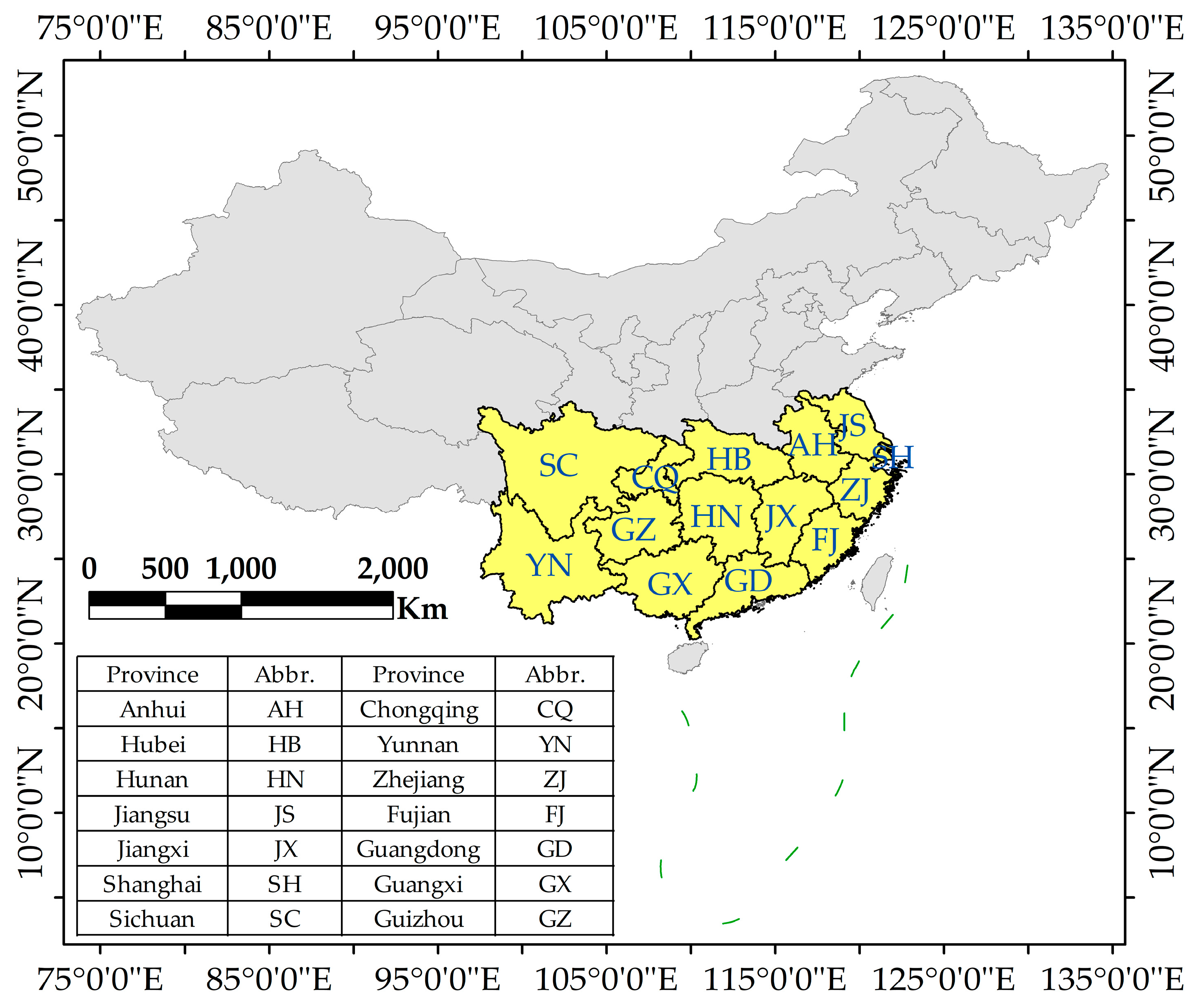
The VIIRS DNB composites for May, June, July, and August contain numerous pixels in high-latitude regions of the northern hemisphere with no data because solar illumination seriously contaminates these regions in the summer months. Fourteen provinces of southern China were selected as study cases in this paper considering the spatial and temporal coverage of monthly VIIRS DNB data, which include Anhui, Hubei, Hunan, Jiangsu, Jiangxi, Shanghai, Sichuan, Chongqing, Yunnan, Zhejiang, Fujian, Guangdong, Guangxi, and Guizhou. Figure 1 showed the distribution of the provinces in the study area.

2.1.2. Nighttime Light Data

The monthly cloud-free composites of VIIRS NTL images collected from December 2012 to January 2019 were used in this study. These images were retrieved from the National Oceanic and Atmospheric Administration National Centers for Environmental Information (https://ngdc.noaa.gov/eog/viirs/index.html, last accessed on 1 April 2019). These data have not been filtered to screen out lights from aurora, fires, boats, and other temporal lights. Only two years of yearly composites released on the website (2016 and 2017). The VIIRS images provide gridded average values of anthropogenic NTL radiance (in units of nW/(cm²·sr) hereafter) with a spatial resolution of 15 arc-seconds (~500 m at the equator).

The NTL data of June 2018 was not available online, which was represented by the average data of May and July 2018. For better identification, the downloaded NTL data and estimated NTL data of June 2018 were identified as original NTL or NTL₀ hereafter.

2.1.3. Auxiliary Data

Monthly EPC data of 14 provinces in study area from January 2013 to December 2018 were acquired from statistical website of each provincial government. EPC included industrial and household electricity consumption, which could reflect the social and economic status.

The vector data of provincial administrative regions of study area was acquired from website of Database of Global Administrative Areas (GADM, https://gadm.org/) will be used for regional aggregation of NTL data. The projection and coordinate of the vector data were consistent with VIIRS DNB data.

2.2. Methods

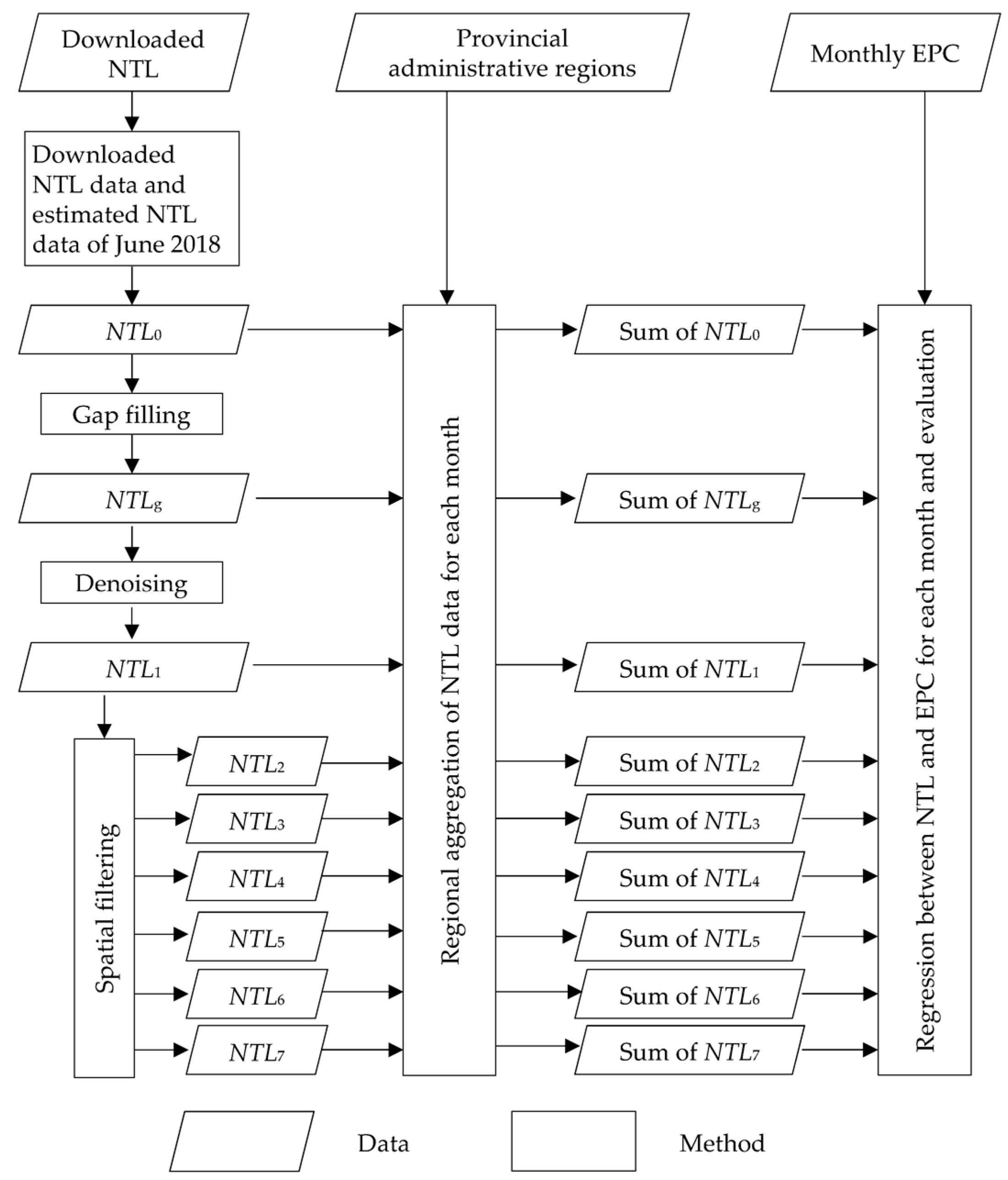
Four main procedures were undertaken to figure out the optimal regression between NTL and EPC: firstly, gap filling of downloaded NTL data; secondly, denoising of gap filled NTL; thirdly, spatial filtering for denoised NTL; fourthly, regression between NTL and EPC for each month and evaluation of regression (Figure 2).

2.2.1. Gap Filling of NTL Data

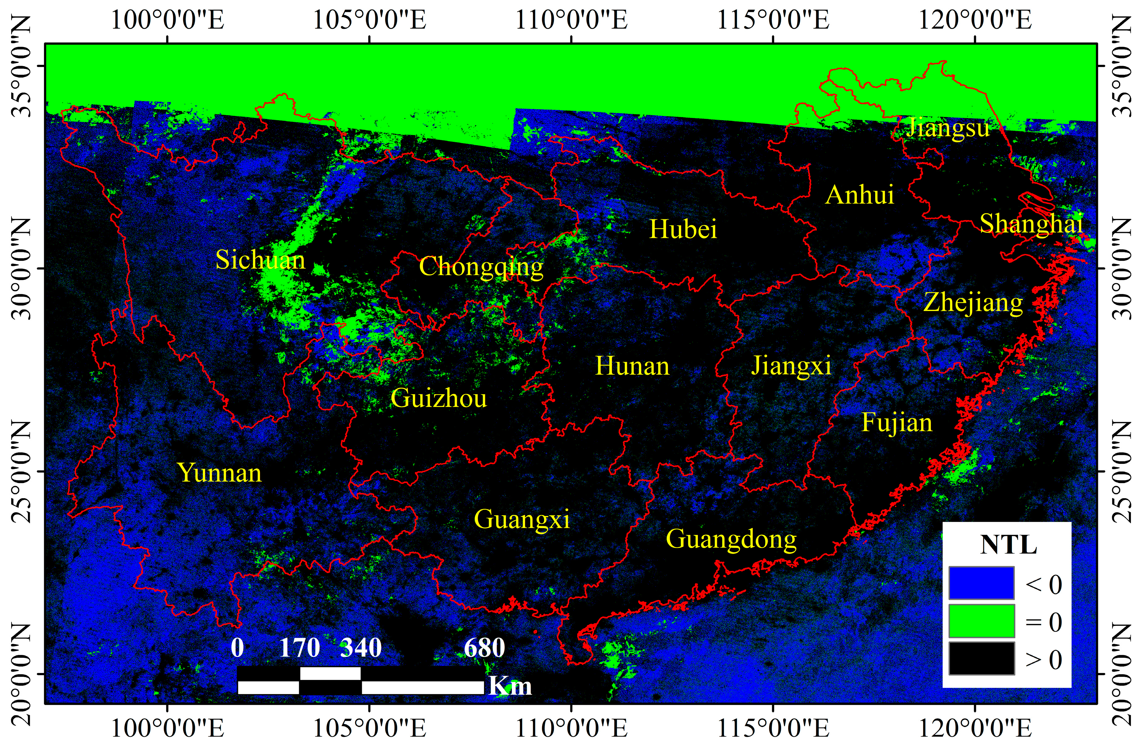
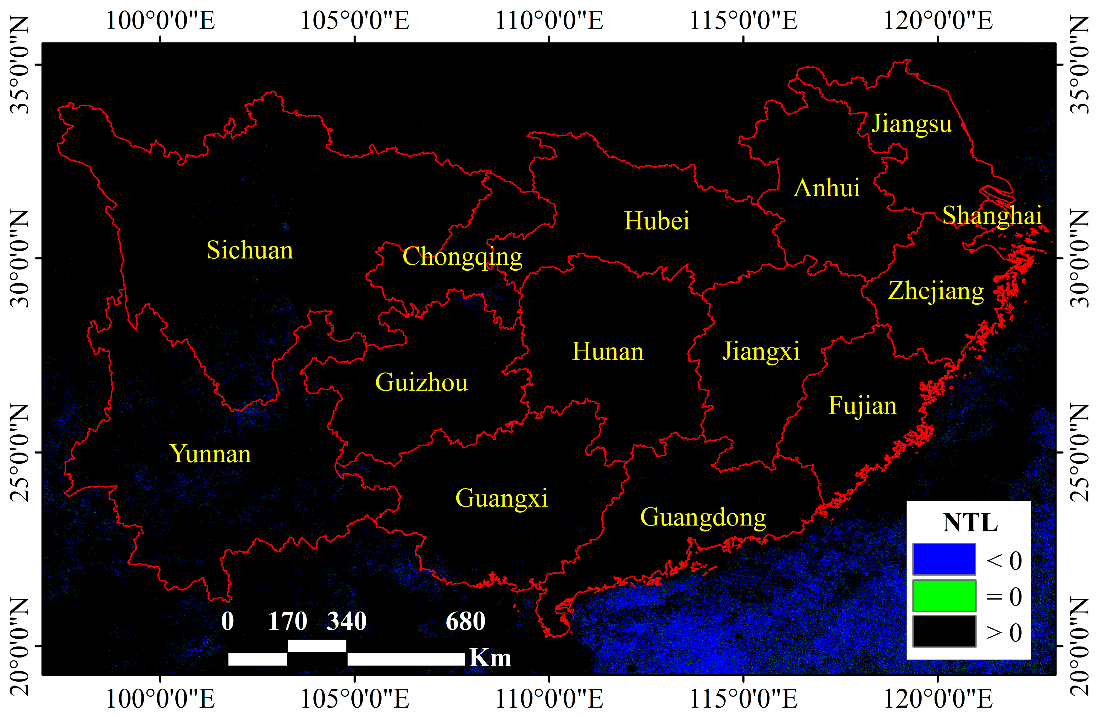
NTL data with nearly complete spatial coverage of study area in all months were selected for experiment. However, there were still no-value areas in the northernmost part of the study area in June every year. These no-value pixels were replaced by the average of the same pixels in May and July of the same year [36]. In addition, due to various factors, pixels with values less than or equal to 0 nW/(cm²·sr) may sporadically appeared in images in all months, which were replaced by the average values of the same pixels in the preceding and the following months based on the assumption that night lighting should be gradually changed between adjacent months. The NTL data of June 2014 before and after gap filling were shown as an example in Figure 3 and Figure 4, respectively. After gap filling, data coverage and availability of NTL data were significantly improved. Nevertheless, there were still a small number of pixels equal to or less than 0 nW/(cm²·sr) in the image, which will be handled in the subsequent noise reduction process.

The NTL data after gap filling for pixels less than or equal to 0 nW/(cm²·sr) was called NTL_g hereafter.

2.2.2. Denoise of NTL

Several kinds of processing were implemented on NTL_g data, including denoising, average filtering, median filtering, and mid-value filtering.

There existed background noise in VIIRS DNB data that should be treated. Li et al. derived a denoised NTL data through multiplying the NPP-VIIRS imagery by the mask generating with all positive value pixels from the DMSP-OLS imagery in 2010 [15]. Ma et al. proposed a simple and feasible method of denoising by taking the mean radiance value of lake pixel samples as the denoising threshold value, which equaled to 0.3 nW/(cm²·sr) [37]. Using the method proposed by Ma et al., the NTL_g data were denoised by setting pixels of value lower than 0.3 nW/(cm²·sr) with 0 nW/(cm²·sr), which were called denoised NTL with threshold of 0.3 hereafter (or NTL₁).

2.2.3. Spatial Filtering

There may be a few pixels with abnormally high value in NTL₁ data, due to gas flares, fires, oilfields, volcanoes, etc. In order to reduce the potential influence of abnormally high values, average filtering, median filtering, and mid-value filtering were implemented on NTL₁, respectively.

Average filtering means that the pixel value is reset to average value of n*n adjacent pixels. The results of average filtering of 3 × 3 and 5 × 5 were called NTL₂ and NTL₃ hereafter, respectively.

Median filtering means that the pixel value is reset to median value of n*n adjacent pixels. The results of median filtering of 3 × 3 and 5 × 5 were called NTL₄ and NTL₅ hereafter, respectively.

Mid-value filtering means that the pixel value is reset to the average of maximum and minimum value of n*n adjacent pixels. The results of mid-value filtering of 3 × 3 and 5 × 5 were called NTL₆ and NTL₇ hereafter, respectively.

2.2.4. Regression and Evaluation

Sum of NTL of each provincial region was calculated for each kind of NTL data (NTL₀-NTL₇ and NTL_g) by accumulating values of all pixels in each region and each month.

Two common regression models, linear regression and polynomial regression, were performed between each sum of NTL and EPC data, respectively.

R-squared mean absolute relative error (MARE), maximum relative error (MRE), and root mean squared error (RMSE) were used to demonstrate the reliability of regression, which were described as

$$RMSE=\sqrt{\frac{1}{m}{{\displaystyle \sum }}_{i=1}^m{\left({\widehat{y}}_i-y_i\right)}^2} ,$$

(1)

$$MRE=\underset{i}{\max }\left(\left|{\widehat{y}}_i-y_i\right|\right) ,$$

(2)

$$MARE=\frac{1}{m}{{\displaystyle \sum }}_{i=1}^m\left|{\widehat{y}}_i-y_i\right|,$$

(3)

where $y_i$ represents statistical EPC data of the ith sample. ${\widehat{y}}_i$ represents calculated EPC data of the ith sample. m denotes the sample size of each month, which equals to 84 in this study.

R square and RMSE were used to evaluate the quality of regression. The higher R square and the lower RMSE were, the stronger the regression will be. MARE and MRE were used to describe the estimation error of models, which were only used as reference parameters due to the fact that maximum R square, minimum RMSE, and minimum MARE may not indispensably occur at the same time.

3. Results

3.1. Overall Analysis of Regression

Two types of regression between monthly EPC and nine kinds of monthly NTL data with different treatments were performed. A total of 216 regression equations were obtained for 12 months. It was essential to decide which kind of regression performed strongest and which kind of NTL data performed best in regression, for the sake of been reliably applied in the future.

As mentioned above, R square, MARE, MRE, and RMSE were employed to describe the quality of each regression equation. In order to compare the stability of these regression analyses in 12 months of a year, the average of regression parameters of each regression in 12 months were calculated and a total of 18 groups of average values were obtained (shown in

Table 1. Mean regression parameters of 12 months for each regression

Types of Regression	Types of NTL (Independent Variable)	R-Square	MARE	MRE	RMSE
Linear regression	Original NTL (NTL0)	0.8459	20.70	100.64	486632.44
	Gap filled (NTLg)	0.8482	19.86	101.41	483911.95
	Denoised by threshold of 0.3 (NTL1)	0.8837	18.24	81.57	418672.05
	3*3 average filtered (NTL2)	0.8836	18.24	81.66	418819.95
	5*5 average filtered (NTL3)	0.8835	18.23	81.83	419025.50
	3*3 median filtered (NTL4)	0.8821	18.46	81.05	421391.10
	5*5 median filtered (NTL5)	0.8799	18.82	82.19	425319.41
	3*3 mid-value filtered (NTL6)	0.8820	18.31	82.36	422168.61
	5*5 mid-value filtered (NTL7)	0.8650	19.80	89.86	451911.06
	Mean	0.8727	18.96	86.95	438650.23
Polynomial regression	Original NTL (NTL0)	0.8607	17.18	92.30	462995.95
	Gap filled (NTLg)	0.8612	16.39	95.16	464088.51
	Denoised by threshold of 0.3 (NTL1)	0.8906	16.02	77.85	405215.84
	3*3 average filtered (NTL2)	0.8904	16.03	78.11	405513.61
	5*5 average filtered (NTL3)	0.8902	16.06	78.53	405991.7
	3*3 median filtered (NTL4)	0.8886	16.47	78.81	408859.26
	5*5 median filtered (NTL5)	0.8861	16.92	79.25	414136.96
	3*3 mid-value filtered (NTL6)	0.8898	15.89	80.05	408297.95
	5*5 mid-value filtered (NTL7)	0.8768	16.49	82.85	432332.95
	Mean	0.8816	16.38	82.55	423048.08

).

According to the average value in Table 1, all 18 regression formulas achieved promising results, with all R square exceeded 0.8459 and mean value of R square equaled to 0.8772. The linear regression between NTL₀ and EPC was comparatively the least reliable one, whose R square, MARE, MRE, and RMSE were 0.8459, 20.70, 100.64, and 486632.44, respectively. Meanwhile, the polynomial regression between NTL₀ and EPC was comparatively the least reliable one in 9 kinds of polynomial regression, whose R square, MARE, MRE, and RMSE were 0.8607, 17.18, 92.30, and 462995.95, respectively. In other words, when linear regression or polynomial regression was performed between EPC data and various NTL data, respectively, using processed NTL data was consistently more reliable than using original NTL data. These comparisons demonstrated the necessity to process NTL data appropriately before using it to estimate EPC, which may improve the reliability of estimation.

As shown in Table 1, polynomial regressions were superior to linear regression in reliability for regressions between any kind of NTL data and EPC. The mean values of R square, MARE, MRE, and RMSE of nine linear regressions were 0.8727, 18.96, 86.95, and 438650.23, respectively. However, the mean values of R square, MARE, MRE, and RMSE of nine polynomial regressions were 0.8816, 16.38, 82.55, and 423048.08, respectively. It was noticeable that the mean value of MARE of polynomial regressions was 13.60%, lower than that of linear regressions. Therefore, compared with linear regression, polynomial regressions can obtain higher precision results in estimating monthly EPC based on NTL data.

Among the nine kinds of NTL data to be based in building regression models, regression between NTL₁ and EPC steadily exhibited the strongest reliability in two types of regressions. The mean value of R square of regressions between NTL₁ and EPC reached the highest value in two types of regression, respectively. By contrast, three kinds of processing (average filtering, median filtering, and mid-value filtering) on NTL₁ data failed to effectively improve the reliability of regression.

Based on the above analysis, the polynomial regressions between NTL₁ and EPC would be mainly concerned in the following sections.

3.2. Analysis of Monthly Regression

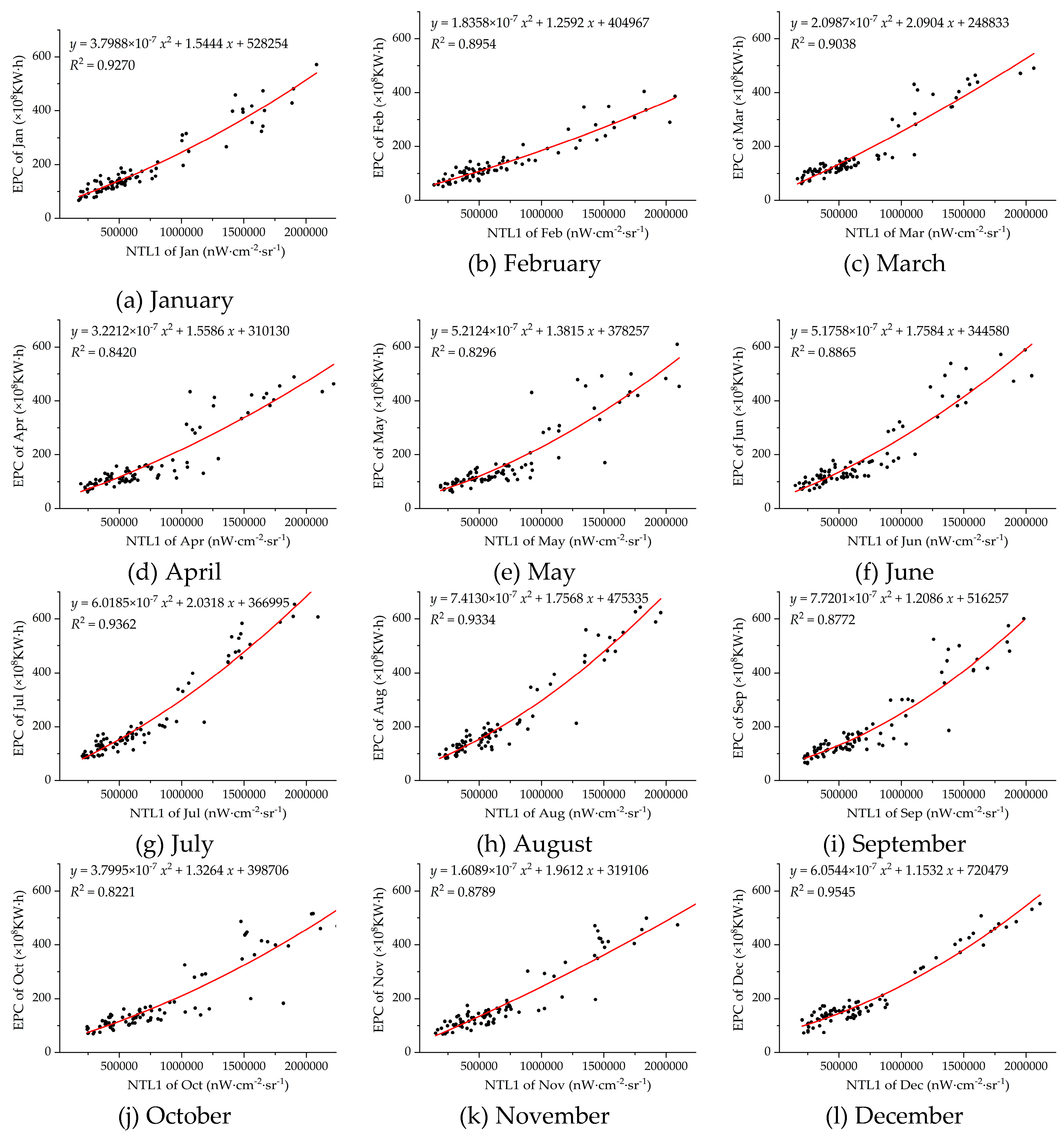
Taking NTL₁ as the independent variable and EPC as the dependent variable, the polynomial regressions of 12 months were built, respectively, and the results were showed in Figure 5.

In each plot, the regression curve visibly reflected the distribution trend of scattered points. The vast majority of the points were close to the fitting curves, whose relative errors were low. Even in polynomial regressions with relatively low R square (Figure 5e,j), only a few points were relatively far from the regression curves, with comparatively higher relative errors.

Polynomial regression equations between NTL₁ and EPC for 12 months, together with corresponding R square, MARE, MRE, and RMSE, were listed in

Table 2. Polynomial regression between NTL₁ and EPC for each month

Month	Regression Formula	R square	MARE	MRE	RMSE
Jan	y = 3.7988×10−7x2 + 1.5444x + 528254	0.9270	12.52	32.20	306976.24
Feb	y = 1.8358×10−7x2 + 1.2592x + 404967	0.8954	14.21	50.58	262870.38
Mar	y = 2.0987×10−7x2 + 2.0904x + 248833	0.9038	15.50	65.75	370635.34
Apr	y = 3.2212×10−7x2 + 1.5586x + 310130	0.8420	19.03	95.45	470503.52
May	y = 5.2124×10−7x2 + 1.3815x + 378257	0.8296	19.53	111.24	538127.72
Jun	y = 5.1758×10−7x2 + 1.7584x + 344580	0.8865	18.23	58.02	453496.40
Jul	y = 6.0185×10−7x2 + 2.0318x + 366995	0.9362	13.26	66.11	388180.76
Aug	y = 7.4130×10−7x2 + 1.7568x + 475335	0.9334	13.27	81.65	399151.08
Sep	y = 7.7201×10−7x2 + 1.2086x + 516257	0.8772	17.24	99.04	471238.43
Oct	y = 3.7995×10−7x2 + 1.3264x + 398706	0.8221	19.10	126.11	519539.28
Nov	y = 1.6089×10−7x2 + 1.9612x + 319106	0.8789	17.37	80.18	418210.36
Dec	y = 6.0544×10−7x2 + 1.1532x + 720479	0.9545	12.94	67.86	263660.58

X refers to NTL₁, in units of nW/(cm²·sr). Y refers to EPC, in units of 10⁴KW·h.

. In the regression of 12 months, the R square of 5 months (Jan, Mar, Jul, Aug, and Dec) were higher than 0.9, together with the MARE lower than 16%. In addition, the R square of 3 months (Apr, May, and Oct) were between 0.82 and 0.85, together with the MARE between 19% and 20%. The MARE described the overall reliability of estimation. However, compared with the MARE, the MRE usually reflects the estimation results of very few abnormal samples, so it does not have a strong co-direction or hetero-direction relationship with R square.

According to the 12 equations listed in Table 2, 84 estimates and corresponding absolute relative errors can be obtained each month. All absolute relative errors were statistically summarized according to 6 intervals ([0, 10%), [10%, 20%), [20%, 30%), [30%, 40%), [40%, 50%)and [50%, +∞)) and the results were listed in

Table 3. Distribution of absolute relative errors

Month	Regression Formula	[0, 10%)	[10%, 20%)	[20%, 30%)	[30%, 40%)	[40%, 50%)	[50%, +∞)
Jan	y = 3.7988×10−7x2 + 1.5444x + 528254	36	31	14	3	0	0
Feb	y = 1.8358×10−7x2 + 1.2592x + 404967	33	31	13	5	1	1
Mar	y = 2.0987×10−7x2 + 2.0904x + 248833	33	22	22	5	1	1
Apr	y = 3.2212×10−7x2 + 1.5586x + 310130	25	31	13	6	5	4
May	y = 5.2124×10−7x2 + 1.3815x + 378257	26	28	17	5	3	5
Jun	y = 5.1758×10−7x2 + 1.7584x + 344580	23	29	22	5	3	2
Jul	y = 6.0185×10−7x2 + 2.0318x + 366995	40	27	10	3	2	2
Aug	y = 7.4130×10−7x2 + 1.7568x + 475335	41	29	7	3	1	3
Sep	y = 7.7201×10−7x2 + 1.2086x + 516257	29	34	12	3	0	6
Oct	y = 3.7995×10−7x2 + 1.3264x + 398706	35	14	22	6	3	4
Nov	y = 1.6089×10−7x2 + 1.9612x + 319106	34	22	13	7	5	3
Dec	y = 6.0544×10−7x2 + 1.1532x + 720479	42	23	14	4	0	1

A total of 84 samples were covered in each regression. This table listed the frequency of occurrence of absolute relative errors in each range.

.

In general, among all 1008 estimations (84 per month, 12 months), the frequency of occurrence of absolute relative error of [0, 10%), [10%, 20%), [20%, 30%), [30%, 40%), [40%, 50%), and [50%, +∞) were 397, 321, 179, 55, 24, and 32 times, respectively, accounting for 39.38%, 31.85%, 17.76%, 5.46%, 2.38%, and 3.17%, respectively. For nearly 90% of the samples, the absolute relative errors between estimated EPC and statistical values were less than 30%, which indicated that high estimation accuracy could be achieved in most cases.

4. Discussion

The reason why so many researchers endeavored to estimate EPC based on NTL images was because the process of consuming electricity was often accompanied by the emission of light, such as home lights, business lights, street lamps, etc. However, not all EPC produced lights, such as air conditioners, water heaters, electric fans, etc. Although these electrical devices did not directly produce lights, they were closely related to human activities. Where there were air conditioners, water heaters, electric fans, and other electrical appliances, there would be human activities, accompanied by household lights, commercial lights, street lamps, and so on. In addition, some other things besides electricity may produce lights, by using gasoline or other materials, such as fireworks, car lights, etc.

From the perspective of time, the data of EPC includes the total EPC in a whole period of time, while the NTL data only records the light information above a certain brightness at a certain moment, which cannot record the information of most other time periods. Therefore, it is theoretically impossible to accurately calculate the annual or monthly EPC by using NTL data. We can only estimate EPC values within a given time period based on composite data of NTL values at multiple moments. The accuracy of estimation may be affected by industrial structure, energy consumption structure, population structure, and other factors in different regions besides the accuracy of NTL data.

The overpass time of SNPP is around 01:30 in local solar time, which is not the peaking lighting time within a day. By visual interpretation upon VIIRS DNB images, there is still plenty of lighting after midnight, which may probably last until dawn. Using such lighting information can reasonably reflect socio-economic activities considering that reliable results have been obtained in large number of previous studies based on this data.

Environmental surface variables may affect nighttime brightness. Levin found that albedo and snow cover exert obvious positive impacts on VIIRS DNB nighttime brightness [38]. The accuracy of estimating socioeconomic activities using VIIRS data may be enhanced if the magnitude of impact can be reasonably estimated and corresponding calibration treatment be performed on VIIRS data.

The probable impacts of satellite observation angles were not covered in this study. Li et al. investigated the variation of viewing angles of SNPP satellite and quantified the viewing angle effects on the artificial light radiance [39]. The VIIRS DNB data will be able to describe socioeconomic activities more accurately if they are improved by removing the angular effects.

Despite the above problems, there is a close positive correlation between EPC and NTL data, which can reflect the social and economic activities of human beings on the surface of the earth to a large extent. The use of NTL data can achieve a long time series, large spatial coverage, rapid monitoring of social and economic activities.

DMSP/OLS data was the most widely used NTL data in EPC estimation, due to its long time series (1992–2013). Despite its advantages, VIIRS DNB data was relatively less used in EPC estimation due to its short time series. Previous studies have shown that annual EPC data can be estimated using VIIRS DNB data with a higher accuracy than DMSP/OLS data. Except for annual data, NOAA released monthly composite VIIRS DNB data from April 2012 to the present. Unfortunately, no study regarding estimating monthly EPC using monthly composite VIIRS DNB data has been reported. We conducted regression analysis between monthly EPC and corresponding monthly composite VIIRS DNB data and obtained satisfactory results. This demonstrated the feasibility of estimating monthly EPC using monthly composite VIIRS DNB data. In addition, NOAA began to release daily VIIRS DNB data, which will provide additional data option for future research.

Linear regression models were often employed in estimating EPC based on NTL data. For each month, we compared polynomial regression model with linear regression model and found that the accuracy of EPC estimation using polynomial regression model was higher than the other one. We also conducted exponential regression and logarithmic regression between EPC and NTL in the experiment, but the R square values were much lower than those of linear regression and polynomial regression.

The method of reducing background noise in NTL data proposed by Ma et al. was employed in this paper, because it was easy to understand and conduct. In spite of noise reduction, there might still be other sources of at-sensor nighttime radiance that remain uncorrected in the dataset, such as atmospheric backscatter and diffuse radiation [40].

The purpose of conducting three kinds of spatial filtering was to reduce the feasible influence of abnormal high pixel value. Filtering windows of 3*3 and 5*5 were chosen because they were widely used and have low computational complexity. However, according to the regression results, the relationships between EPC and spatially filtered NTL data did not improve. This might be due to two reasons: (1) spatial filtering of a small number of outliers had little effect on the total NTL value of the province; (2) a large number of pixels in urban and suburban areas have been smoothed, might resulted in some information loss.

Although we have obtained EPC estimation models based on VIIRS NTL data on a monthly basis, these models are built based on statistical analysis, and it is difficult to explain the physical meaning of each parameter of the models. This is the inherent defect of statistical analysis. However, statistical model is still of practical value and significance before the physical model is established effectively.

In this paper, monthly regression models are established with sample data from 14 provinces in southern China. The parameters of these models may not be appropriate elsewhere, due to different statistical standard of electric power consumption. However, it is feasible to establish monthly regression models for each region using the steps and data described in this paper.

5. Conclusions

This paper investigated the relationship between EPC and NTL data on a monthly scale, using monthly VIIRS DNB NTL composite data from January 2013 to December 2018 and the corresponding monthly statistical data of EPC of 14 provinces in southern China. Two kinds of regressions were compared for the purpose of obtaining more reliable regression results. Furthermore, nine kinds of NTL with different treatments, including original NTL (NTL₀), Gap filled NTL (NTL_g), denoised NTL by threshold of 0.3 (NTL₁), 3*3 average filtered NTL (NTL₂), 5*5 average filtered NTL (NTL₃), 3*3 median filtered NTL (NTL₄), 5*5 median filtered NTL (NTL₅), 3*3 mid-value filtered NTL (NTL₆) and 5*5 mid-value filtered NTL (NTL₇), were involved in building regression formulas. The conclusions are drawn as follows:

High reliability was achieved in all 18 regression formulas (two types of regressions between EPC and nine kinds of processed NTL), with all R square exceeded 0.8459 and mean value of R square equaled to 0.8772. Compared with linear regressions, polynomial regressions acquired higher reliability, whose average R square was 0.8816, higher than 0.8727 of linear regressions. Regressions between denoised NTL with threshold of 0.3 (NTL₁) and EPC steadily exhibited the strongest reliability among the nine kinds of NTL data to be based in building two types of regression models. Three kinds of treatments (average filtering, median filtering, and mid-value filtering) on NTL₁ data did not effectively improve the reliability of regressions. These kinds of data processing were not recommended in estimating EPC based on NTL data.

For the 12 months of polynomial regressions between NTL₁ and EPC, the average value of R square was 0.8906, and the average value of MARE was 16.02%. For nearly 90% of the 1008 estimations (84 per month, 12 months), the absolute relative errors between estimated EPC and statistical values were less than 30%, which indicated high estimation accuracy in most cases.

References

- Elvidge, C.D.; Baugh, K.E.; Kihn, E.A.; Kroehl, H.W.; Davis, E.R.; Davis, C.W. Relation between satellite observed visible-near infrared emissions, population, economic activity and electric power consumption. Int. J. Remote Sens. 1997, 18, 1373–1379. [Google Scholar] [CrossRef]
- Small, C.; Pozzi, F.; Elvidge, C.D. Spatial analysis of global urban extent from DMSP-OLS night lights. Remote Sens. Environ. 2005, 96, 277–291. [Google Scholar] [CrossRef]
- Li, X.; Elvidge, C.; Zhou, Y.; Cao, C.; Warner, T. Remote sensing of night-time light. Int. J. Remote Sens. 2017, 38, 5855–5859. [Google Scholar] [CrossRef] [Green Version]
- Doll, C.; Muller, J.P.; Morley, J.G. Mapping regional economic activity from night-time light satellite imagery. Ecol. Econ. 2006, 57, 75–92. [Google Scholar] [CrossRef]
- Bennett, M.M.; Smith, L.C. Advances in using multitemporal night-time lights satellite imagery to detect, estimate, and monitor socioeconomic dynamics. Remote Sens. Environ. 2017, 192, 176–197. [Google Scholar] [CrossRef]
- Shi, K.; Yu, B.; Huang, Y.; Hu, Y.; Yin, B.; Chen, Z.; Chen, L.; Wu, J. Evaluating the ability of NPP-VIIRS nighttime light data to estimate the gross domestic product and the electric power consumption of China at multiple scales: A comparison with DMSP-OLS data. Remote Sens. 2014, 6, 1705–1724. [Google Scholar] [CrossRef] [Green Version]
- Amaral, S.; Monteiro, A.M.V.; Camara, G.; Quintanilha, J.A. DMSP/OLS night-time light imagery for urban population estimates in the Brazilian amazon. Int. J. Remote Sens. 2006, 27, 855–870. [Google Scholar] [CrossRef]
- Zhou, Y.; Li, X.; Asrar, G.R.; Smith, S.J.; Imhoff, M. A global record of annual urban dynamics (1992–2013) from nighttime lights. Remote Sens. Environ. 2018, 219, 206–220. [Google Scholar] [CrossRef]
- Yu, B.; Tang, M.; Wu, Q.; Yang, C.; Deng, S.; Shi, K.; Peng, C.; Wu, J.; Chen, Z. Urban Built-Up area extraction from Log-Transformed NPP-VIIRS nighttime light composite data. IEEE Geosci. Remote S. 2018, 15, 1279–1283. [Google Scholar] [CrossRef]
- Ma, T. Multi-Level relationships between Satellite-Derived nighttime lighting signals and social media–derived human population dynamics. Remote Sens. 2018, 10, 1128. [Google Scholar] [CrossRef] [Green Version]
- Li, X.; Zhao, L.; Han, W.; Faouzi, B.; Washaya, P.; Zhang, X.; Jin, H.; Wu, C. Evaluating Algeria’s Social and Economic Development Using a Series of Night-Time Light Images Between 1992 to 2012. Int. J. Remote Sens. 2018, 39, 9228–9248. [Google Scholar] [CrossRef]
- Zhao, N.; Zhang, W.; Liu, Y.; Samson, E.L.; Chen, Y.; Cao, G. Improving nighttime light imagery with Location-Based social media data. IEEE T. Geosci. Remote 2019, 57, 2161–2172. [Google Scholar] [CrossRef]
- Elvidge, C.D.; Zhizhin, M.; Baugh, K.; Hsu, F.C.; Ghosh, T. Extending nighttime combustion source detection limits with short wavelength VIIRS data. Remote Sens. 2019, 11, 395. [Google Scholar] [CrossRef] [Green Version]
- Xie, Y.; Weng, Q.; Fu, P. Temporal variations of artificial nighttime lights and their implications for urbanization in the conterminous United States, 2013–2017. Remote Sens. Environ. 2019, 225, 160–174. [Google Scholar] [CrossRef]
- Li, X.; Xu, H.; Chen, X.; Li, C. Potential of NPP-VIIRS nighttime light imagery for modeling the regional economy of China. Remote Sens. 2013, 5, 3057–3081. [Google Scholar] [CrossRef] [Green Version]
- Wu, J.; Wang, Z.; Li, W.; Peng, J. Exploring factors affecting the relationship between light consumption and GDP based on DMSP/OLS nighttime satellite imagery. Remote Sens. Environ. 2013, 134, 111–119. [Google Scholar] [CrossRef]
- Chen, X.; Nordhaus, W.; Elvidge, C.D.; Nichol, J.; Prasad, S.T. A test of the new VIIRS lights data set: Population and economic output in Africa. Remote Sens. 2015, 7, 4937–4947. [Google Scholar] [CrossRef] [Green Version]
- Yu, S.; Zhang, Z.; Liu, F. Monitoring population evolution in China using time-series DMSP/OLS nightlight imagery. Remote Sens. 2018, 10, 194. [Google Scholar] [CrossRef] [Green Version]
- Yu, B.; Lian, T.; Huang, Y.; Yao, S.; Ye, X.; Chen, Z.; Yang, C.; Wu, J. Integration of nighttime light remote sensing images and taxi GPS tracking data for population surface enhancement. Int. J. Geogr. Inf. Sci. 2019, 33, 687–706. [Google Scholar] [CrossRef]
- Zhao, M.; Cheng, W.; Zhou, C.; Li, M.; Huang, K.; Wang, N. Assessing spatiotemporal characteristics of urbanization dynamics in southeast Asia using time series of DMSP/OLS nighttime light data. Remote Sens. 2018, 10, 47. [Google Scholar] [CrossRef] [Green Version]
- Huang, X.; Schneider, A.; Friedl, M.A. Mapping sub-pixel urban expansion in China using MODIS and DMSP/OLS nighttime lights. Remote Sens. Environ. 2016, 175, 92–108. [Google Scholar] [CrossRef]
- Shi, K.; Yang, Q.; Fang, G.; Yu, B.; Chen, Z.; Yang, C.; Wu, J. Evaluating spatiotemporal patterns of urban electricity consumption within different spatial boundaries: A case study of Chongqing, China. Energy 2019, 167, 641–653. [Google Scholar] [CrossRef]
- Xie, Y.; Weng, Q. Detecting urban-scale dynamics of electricity consumption at Chinese cities using time-series DMSP-OLS (Defense Meteorological Satellite Program-Operational Linescan System) nighttime light imageries. Energy 2016, 100, 177–189. [Google Scholar] [CrossRef]
- Townsend, A.C.; Bruce, D.A. The use of night-time lights satellite imagery as a measure of Australia’s regional electricity consumption and population distribution. Int. J. Remote Sens. 2010, 31, 4459–4480. [Google Scholar] [CrossRef]
- Hu, Z.; Hu, H.; Huang, Y. Association between nighttime artificial light pollution and sea turtle nest density along Florida coast: A geospatial study using VIIRS remote sensing data. Environ. Pollut. 2018, 239, 30–42. [Google Scholar] [CrossRef]
- Butt, M.J. Estimation of light pollution using satellite remote sensing and geographic information system techniques. Gisci. Remote Sens. 2012, 49, 609–621. [Google Scholar] [CrossRef]
- Han, P.; Huang, J.; Li, R.; Wang, L.; Hu, Y.; Wang, J.; Huang, W. Monitoring trends in light pollution in China based on nighttime satellite imagery. Remote Sens. 2014, 6, 5541–5558. [Google Scholar] [CrossRef] [Green Version]
- Shi, K.; Chen, Y.; Yu, B.; Xu, T.; Chen, Z.; Liu, R.; Li, L.; Wu, J. Modeling spatiotemporal CO2 (carbon dioxide) emission dynamics in China from DMSP-OLS nighttime stable light data using panel data analysis. Appl. Energy 2016, 168, 523–533. [Google Scholar] [CrossRef]
- Zhao, J.; Ji, G.; Yue, Y.; Lai, Z.; Chen, Y.; Yang, D.; Yang, X.; Wang, Z. Spatio-temporal dynamics of urban residential CO2 emissions and their driving forces in China using the integrated two nighttime light datasets. Appl. Energy 2019, 235, 612–624. [Google Scholar] [CrossRef]
- Li, X.; Li, D. Can night-time light images play a role in evaluating the Syrian crisis? Int. J. Remote Sens. 2014, 35, 6648–6661. [Google Scholar] [CrossRef]
- Li, X.; Liu, S.; Jendryke, M.; Li, D.; Wu, C. Night-time light dynamics during the Iraqi civil war. Remote Sens. 2018, 10, 858. [Google Scholar] [CrossRef] [Green Version]
- Chand, T.R.K.; Badarinath, K.V.S.; Elvidge, C.D.; Tuttle, B.T. Spatial characterization of electrical power consumption patterns over India using temporal DMSP-OLS night-time satellite data. Int. J. Remote Sens. 2009, 30, 647–661. [Google Scholar] [CrossRef]
- He, C.; Ma, Q.; Liu, Z.; Zhang, Q. Modeling the spatiotemporal dynamics of electric power consumption in mainland China using saturation-corrected DMSP/OLS nighttime stable light data. Int. J. Digit. Earth 2014, 7, 993–1014. [Google Scholar] [CrossRef]
- Xie, Y.; Weng, Q. World energy consumption pattern as revealed by DMSP-OLS nighttime light imagery. Gisci. Remote Sens. 2016, 53, 265–282. [Google Scholar] [CrossRef]
- Falchetta, G.; Noussan, M. Interannual variation in night-time light radiance predicts changes in national electricity consumption conditional on income-level and region. Energies 2019, 12, 456. [Google Scholar] [CrossRef] [Green Version]
- Zhao, N.; Hsu, F.; Cao, G.; Samson, E.L. Improving accuracy of economic estimations with VIIRS DNB image products. Int. J. Remote Sens. 2017, 38, 5899–5918. [Google Scholar] [CrossRef]
- Ma, T.; Zhou, C.; Pei, T.; Haynie, S.; Fan, J. Responses of Suomi-NPP VIIRS-derived nighttime lights to socioeconomic activity in China’s cities. Remote Sens. Lett. 2014, 5, 165–174. [Google Scholar] [CrossRef]
- Levin, N. The impact of seasonal changes on observed nighttime brightness from 2014 to 2015 monthly VIIRS DNB composites. Remote Sens. Environ. 2017, 193, 150–164. [Google Scholar] [CrossRef]
- Li, X.; Ma, R.; Zhang, Q.; Li, D.; Liu, S.; He, T.; Zhao, L. Anisotropic characteristic of artificial light at night—Systematic investigation with VIIRS DNB multi-temporal observations. Remote Sens. Environ. 2019, 233, 111357. [Google Scholar] [CrossRef]
- Roman, M.O.; Wang, Z.; Sun, Q.; Kalb, V.; Miller, S.D.; Molthan, A.; Schultz, L.; Bell, J.; Stokes, E.C.; Pandey, B.; et al. NASA’s Black Marble nighttime lights product suite. Remote Sens. Environ. 2018, 210, 113–143. [Google Scholar] [CrossRef]
Figure 1.
Study area. Fourteen provinces of southern China were selected as study cases considering the spatial and temporal coverage of monthly VIIRS DNB data.
Figure 2.
Flowchart of methodology.
Figure 3.
NTL of study area in June 2014. June is the month with minimum spatial coverage of NTL data within a year. The continuous green areas in north part of the image (north area of Jiangsu, Anhui, and Sichuan provinces) are areas with null value.
Figure 4.
NTL of study area in June 2014 after gap filling.
Figure 5.
Polynomial regression between NTL1 and EPC for each month. Panel (a)–(l) represents the regression of January to December, respectively. The x-axis refers to NTL1 in units of nW/(cm2·sr). The y-axis refers to EPC in units of 108KW·h.