


Abstract
We have selected a homogeneous sample of asymptotic giant branch (AGB) stars in the Galactic bulge population from the ISOGAL survey. Our target stars cover a wide range of mass-loss rates (∼10−8–10−4 M⊙ yr−1) and differ primarily by their age on the AGB. This homogeneous sample is thus ideally suited to study the dust formation process as a function of age on the AGB. We observed our sample with Spitzer-Infrared Spectrograph, and studied the overall properties of the infrared spectra of these targets. The analysis is complicated by the presence of strong and variable background emission, and the extracted infrared AGB star spectra are affected by interstellar extinction. Several stars in our sample have no detectable dust emission, and we used these ‘naked stars’ to characterize the stellar and molecular contributions to the infrared spectra of our target stars. The resulting dust spectra of our targets do indeed show significant variety in their spectral appearance, pointing to differing dust compositions for the targets. We classify the spectra based on the shape of their 10-μm emission following the scheme by Sloan & Price. We find that the early silicate emission classes associated with oxide dust are generally under-represented in our sample due to extinction effects. We also find a weak 13-μm dust feature in two of our otherwise naked star spectra, suggesting that the carrier of this feature could potentially be the first condensate in the sequence of dust condensation.
1 INTRODUCTION
In the dust (and gas) budget of the galaxy, stars on the asymptotic giant branch (AGB) play a major role (see Iben & Renzini 1983; Habing 1996; Herwig 2005, for reviews about various aspects of AGB phase). During this stellar phase, stars with initial masses between ∼0.8 and 8 M⊙ lose much of their mass through a dust-driven wind, and eventually end up as slowly cooling white dwarfs with core masses within ∼0.5–1.4M⊙ (see e.g. Kalirai et al. 2008; Marigo 2013). In fact, while the details are not well understood, the evolution of the star in this phase is thought to be dominated by mass-loss from the surface rather than nuclear burning in the interior. The mass-loss process on the AGB is thought to be initiated by stellar pulsations which transport material high above the photosphere while it cools down, allowing small dust particles to nucleate and grow. Radiation pressure rapidly accelerates these dust grains and the gas is dragged along. This results in slow (5–20 km s−1), massive (10−8–10−4 M⊙ yr−1) outflows which last for some 106 yr, amounting to 0–0.07 M⊙ of dust (and 0.3–7 M⊙ of gas; Willson 2000; Girardi et al. 2013).
As a result of this mass-loss, the IR spectral appearance of AGB stars – as well as their evolutionary ‘daughters’, the post-AGB objects and planetary nebulae – is dominated by the dust ejected during the AGB phase. Previous space-based studies (IRAS and ISO) have revealed a large variety of dust materials in these types of objects, including aluminium oxides (Miyata et al. 2000; Cami 2002), magnesium–iron oxides (Cami 2002; Posch et al. 2002), and various crystalline and amorphous silicates (for a review on ISO results, see Blommaert et al. 2005). However, while there is some observational evidence that these compositional variations are related to the mass-loss rate, the origin of these variations and the physical and chemical processes driving this complexity are not well understood.
Stardust forms through chemical nucleation and growth in cool (∼1000 K), dense (∼108 cm−3) gas. Theoretical studies on dust formation have a long history in astrophysics dating back to Salpeter (1974) for stellar ejecta and Grossman & Larimer (1974) for the solar nebula. These and subsequent studies (Sedlmayr 1989; Kozasa & Sogawa 1997) rely on thermodynamic condensation sequences to predict the compounds formed and the fraction of mass locked up in them. For O-rich ejecta, these thermodynamic studies predict that dust formation starts with the formation of very refractory oxides (aluminium oxide, spinel) at a temperature of ∼1500 K. Through a variety of gas–solid and solid–solid interactions, these compounds are then transformed into calcium–aluminium silicates when the outflowing gas cools further. At about 1200 K, the majority of the silicon will condense first as magnesium-rich olivine (forsterite, Mg2SiO4), which reacts with excess gaseous silicon to transform into pyroxene (enstatite, MgSiO3).
There is qualitative confirmation of these predictions for dust formation in stellar ejecta. Several observations, mostly Infrared Astronomical Satellite (IRAS)/Low Resolution Spectrometer (LRS) and ISO/Short Wavelength Spectrometer (SWS), have revealed the presence of many different dust compounds in O-rich AGB stars (Vardya, de Jong & Willems 1986; Onaka, de Jong & Willems 1989; Sloan & Price 1995; Waters et al. 1996; Speck et al. 2000; Fabian et al. 2001; Cami 2002; Posch et al. 2002; Blommaert et al. 2006) and many – but not all – of these compounds are part of the theoretical condensation sequence. Indeed, AGB stars with high mass-loss rates show copious amounts of silicates, including crystalline olivines and pyroxenes. The spectra of AGB stars with low mass-loss rates, on the other hand, only show evidence for spinel, aluminium oxide and magnesium–iron oxides (Blommaert et al. 2006; Karovicova et al. 2013). This difference in spectral structure of AGB stars is thought to reflect the rapid ‘freeze-out’ of the dust condensation sequence, a term used to indicate that the densities in the dust formation zone are too low for certain condensation reactions to occur, and therefore the dust condensation sequence stops at an intermediate step.
Thus, studying a sample of similar stars but with different mass-loss rates is a powerful way to probe the dust condensation sequence observationally, as the freeze-out will occur at different densities and therefore stop the condensation sequence at different intermediate steps. The Galactic bulge offers an interesting opportunity to select such a sample, and the sensitivity of the SpitzerSpace Telescope allows one to study Galactic bulge AGB stars in great detail.
The homogeneity and completeness of our sample can be ensured by carefully selecting stars which have been detected by the ISOGAL survey (Omont et al. 2003). ISOGAL is the second largest survey programme performed with the ISO satellite (Kessler et al. 1996) and provides a point source catalogue in five wavelength bands and includes near-infrared (DENIS; Epchtein et al. 1999), 7- and 15-μm photometry. This survey covered about 16 square degrees in the inner galaxy down to a sensitivity of 10–20 mJy in the mid-infrared and ∼105 sources were detected which are mostly AGB stars, red giants and Young Stellar Objects (YSOs). The survey is complete for sources which are brighter than 9 mag at 7 μm and 8 mag at 15 μm (Omont et al. 2003).
An interesting subset are those ISOGAL sources from fields in the ‘intermediate’ Galactic bulge (|l| < 2° and |b| ≈ 1°–4°). Stars at these latitudes in the direction of the bulge are believed to belong to the bulge stellar population which only shows a small range in masses. These giants have evolved from a population of stars of ≈1.5–2 M⊙ (Groenewegen & Blommaert 2005; Blommaert et al. 2006). Omont et al. (1999) and later Ojha et al. (2003) demonstrated that all sources detected in these fields are AGB stars or stars at the tip of the red giant branch, and that the ISOGAL Ks, 0 − [15] colours can be translated into mass-loss rates (see Fig. 1). Radiative transfer modelling of a subset of ISOGAL sources for which Infrared Space Observatory Camera (ISOCAM) and Circular Variable Filters (CVF) (5–17-μm) data were available (Blommaert et al. 2006) showed that the lowest mass-loss rates detected are ≳ 10−8 M⊙ yr−1. As the ISOGAL sample is complete in terms of magnitudes, it is also complete for the lowest mass-loss rates ( ≳ 10−8 M⊙ yr−1); therefore, AGB stars from the Galactic bulge which are detected in the ISOGAL sample cover the full range of mass-loss rates. It starts from the onset of dusty mass-loss (∼10−8 M⊙ yr−1) and covers up to the mass-loss rates of ∼10−4 M⊙ yr−1 associated with the so-called superwind phase in OH/IR-type AGB stars (see e.g. van Loon et al. 2003).
![[15]/Ks, o−[15] colour–magnitude diagrams for all sources detected in our selected ISOGAL fields (left-hand panel) showing a linear sequence of increasingly redder colours (and thus mass-loss rates) for brighter 15 μm. The right-hand panel shows the representative sample that we have selected. For comparison, we show three tracks corresponding to AGB stars with luminosities of 2000, 4000 and 10 000 L⊙ (bottom, middle and top curve, respectively) and with mass-loss rates increasing from 10−9 to 3 × 10⁻⁶ M⊙ yr−1 (squares on the 4000 L⊙ track indicate mass-loss rates of 10−9, 10−8, 5× 10⁻⁸, 10−7, 5 × 10⁻⁷, 10−6 and 3× 10⁻⁶ M⊙ yr−1). The tracks were obtained using a mixture of amorphous silicate and aluminium oxide dust (see Groenewegen 1993, 1995, for the radiative transfer models). The vertical dot–dashed line represents a track of increasing luminosity without mass-loss. Note that the six OH/IR stars in our sample that were selected from IRAS have no corresponding 2MASS and ISOGAL fluxes and are therefore not shown in this CMD [figures taken from Blommaert et al. (2006), with permission] (Skrutskie, Cutri & Stiening 2006).](https://oup.silverchair-cdn.com/oup/backfile/Content_public/Journal/mnras/443/4/10.1093_mnras_stu1317/2/m_stu1317fig1.jpeg?Expires=1716404654&Signature=4cuXEDb79okoCeSb0NKSp3RhaqlZ2kc7FBj2JCbYAb1Nol-fWbIIhf20SN9NfRW08B8y8OryyO8MhRLwqC3~Xf~iUbHV390UhrjCZbjpo-upH3bQWni1pg3ZCC6TjmCl~GDLav9IRIqIR3tS62rJwRcUYs3WL578XVI5sr098KD1cZGnDUiU0yf4CI6LlrYhcnJM0A9KehXCxGHRbB6JoKlWpRbONJGIJayyhB6Usq92nPv8hk9cLHf7bBkCdciyNDQs1OaUG5vc1rHk7CqGhtTtNLYqLGNJm0T934RWvjX1hXhdpU2wreEyFN4wDP-n65VcxzwlZSpcyfHzr0P5sA__&Key-Pair-Id=APKAIE5G5CRDK6RD3PGA)
[15]/Ks, o−[15] colour–magnitude diagrams for all sources detected in our selected ISOGAL fields (left-hand panel) showing a linear sequence of increasingly redder colours (and thus mass-loss rates) for brighter 15 μm. The right-hand panel shows the representative sample that we have selected. For comparison, we show three tracks corresponding to AGB stars with luminosities of 2000, 4000 and 10 000 L⊙ (bottom, middle and top curve, respectively) and with mass-loss rates increasing from 10−9 to 3 × 10⁻⁶ M⊙ yr−1 (squares on the 4000 L⊙ track indicate mass-loss rates of 10−9, 10−8, 5× 10⁻⁸, 10−7, 5 × 10⁻⁷, 10−6 and 3× 10⁻⁶ M⊙ yr−1). The tracks were obtained using a mixture of amorphous silicate and aluminium oxide dust (see Groenewegen 1993, 1995, for the radiative transfer models). The vertical dot–dashed line represents a track of increasing luminosity without mass-loss. Note that the six OH/IR stars in our sample that were selected from IRAS have no corresponding 2MASS and ISOGAL fluxes and are therefore not shown in this CMD [figures taken from Blommaert et al. (2006), with permission] (Skrutskie, Cutri & Stiening 2006).
With all the stars in these fields originating from about 1.5 M⊙ stars, the main difference between these objects is their age on the AGB, and colour–magnitude diagrams (CMD) of these stars as the one presented in Fig. 1 effectively correspond to the evolutionary track on the AGB for a 1.5 M⊙ star, characterized by varying luminosities and mass-loss rates (see e.g. Girardi et al. 2010). These fields therefore offer unique opportunities to study the evolution of 1.5 M⊙ stars and their circumstellar material as they evolve on the AGB.
Here, we present a first analysis of Spitzer observations of a sample of AGB stars, selected from these bulge fields. This sample is the core of an observational programme whose main scientific goal is to study the variations in the dust composition as a function of mass-loss rate and other fundamental stellar parameters. We present the selection criteria and the sample of stars in Section 2. The Spitzer-Infrared Spectrograph (Spitzer-IRS) observations and the data reduction steps are detailed in Section 3. In Section 4, we describe the strong and variable emission of interstellar dust that contaminates our observations. In Section 5, we describe the spectra, and focus in particular on the ‘naked stars’ – objects without dust emission. These prove particularly useful to characterize the contribution of the star and the molecular layers to the infrared spectra, and to assess the effect of interstellar extinction in Section 6. We characterize our sample in Section 7 and present the resulting dust emission spectra in Section 8. We summarize our findings in Section 9.
2 THE SAMPLE SELECTION
ISO/SWS studies of nearby O-rich AGB stars have revealed the presence of at least five distinct dust components in the wavelength range 8–27 μm (see e.g. Cami 2002), and several more features at wavelengths longer than 30 μm (an overview can be found in Blommaert et al. 2005). Typically, oxide dust dominates the spectra of stars with low mass-loss rates, while high mass-loss rate objects exhibit strong silicate emission (SE). From these differences in the dust composition and given the range in mass-loss rates for these objects, we estimate that we need a sample of ∼15 sources per logarithmic bin in mass-loss rate to fully sample these variations in a statistically significant way.
Ojha et al. (2003) and Blommaert et al. (2006) showed that the Ks, o − [15] colour is a good tracer for mass-loss rates for AGB stars in the ISOGAL fields (see also Fig. 1). We therefore selected our targets based on their Ks, o − [15] colour. We included sources with Ks, o − [15] values close to zero to ensure that we can trace the dust at the onset of mass-loss. From the bulge fields in the ISOGAL sample (c32, c35, the Ogle field and NGC 6522), we thus selected 47 sources. We also included OH/IR stars to represent the highest mass-loss rates on the AGB. Since the superwind phase is extremely short (less than 10 000 yr), OH/IR stars are rare in the ISOGAL bulge fields and we therefore have included six OH/IR stars detected with IRAS, to complete our sample on the high mass-loss rate end. These OH/IR stars were selected from the same latitude range as our ISOGAL sources and have similar luminosities as the Miras in our sample. Thus, we expect that these OH/IR stars belong to the same population. Our final sample of 53 sources then cover ∼4 orders of magnitude in mass-loss rate (10−8–10−4 M⊙ yr−1). The complete list of our sample targets is presented in Table 1; their position in Galactic coordinates is indicated in Fig. 2.
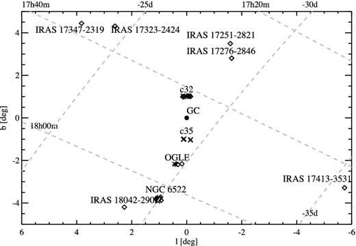
The location of our targets in Galactic coordinates. Note that targets in c32 and c35 are at roughly the same angular distance (about 1 deg) to the Galactic Centre.
Basic data for our sample of Galactic bulge AGB stars (Skrutskie et al. 2006).
| ID | Objecta | RA | Dec. | b | l | J | H | Ks | [7] | [15] | AOR key |
|---|---|---|---|---|---|---|---|---|---|---|---|
| [J2000] | [J2000] | (deg) | (deg) | (mag) | (mag) | (mag) | (mag) | (mag) | |||
| c32-1 | J174117.5−282957 | 17:41:17.50 | −28:29:57.5 | 1.037 | 359.874 | 9.702 | 7.872 | 6.996 | 5.36 | 4.42 | 10421504 |
| c32-2 | J174122.7−283146 | 17:41:22.70 | −28:31:47.0 | 1.005 | 359.858 | - | – | – | 3.47 | 1.54 | 10421504 |
| c32-3 | J174123.6−282723 | 17:41:23.56 | −28:27:24.2 | 1.041 | 359.922 | 10.715 | 8.993 | 8.245 | 7.57 | 6.98 | 10422784 |
| c32-4 | J174126.6−282702 | 17:41:26.60 | −28:27:02.2 | 1.034 | 359.933 | 11.557 | 9.285 | 7.895 | 5.44 | 3.83 | 10421504 |
| c32-5 | J174127.3−282851 | 17:41:27.26 | −28:28:52.1 | 1.016 | 359.908 | 10.008 | 8.306 | 7.304 | 5.78 | 4.40 | 10421504 |
| c32-6 | J174127.9−282816 | 17:41:27.88 | −28:28:17.1 | 1.019 | 359.918 | 9.569 | 7.828 | 7.016 | 6.30 | 5.24 | 10421504 |
| c32-7 | J174128.5−282733 | 17:41:28.51 | −28:27:33.8 | 1.024 | 359.929 | 9.580 | 7.968 | 7.107 | 6.41 | 5.34 | 10421504 |
| c32-8 | J174130.2−282801 | 17:41:30.15 | −28:28:01.3 | 1.015 | 359.926 | 11.353 | 9.662 | 8.880 | 7.77 | 7.44 | 10422784 |
| c32-9 | J174134.6−282431 | 17:41:34.60 | −28:24:31.4 | 1.032 | 359.984 | 10.902 | 9.137 | 8.163 | 5.97 | 4.87 | 10421504 |
| c32-10 | J174139.5−282428 | 17:41:39.48 | −28:24:28.2 | 1.017 | 359.994 | 9.528 | 7.801 | 6.874 | 5.34 | 4.00 | 10421504 |
| c32-11 | J174140.0−282521 | 17:41:39.94 | −28:25:21.2 | 1.008 | 359.982 | 9.630 | 7.977 | 7.143 | 6.09 | 4.15 | 10421504 |
| c32-12 | J174155.3−281638 | 17:41:55.27 | −28:16:38.7 | 1.037 | 0.135 | 9.610 | 7.739 | 6.785 | 5.61 | 3.91 | 10421504 |
| c32-13 | J174157.6−282237 | 17:41:57.53 | −28:22:37.7 | 0.977 | 0.055 | 9.852 | 8.272 | 7.438 | 6.74 | 5.18 | 10421504 |
| c32-14 | J174158.8−281849 | 17:41:58.73 | −28:18:49.2 | 1.007 | 0.111 | 10.160 | 8.415 | 7.348 | 5.57 | 3.85 | 10421504 |
| c32-15 | J174203.7−281729 | 17:42:03.69 | −28:17:29.9 | 1.003 | 0.139 | 10.262 | 8.501 | 7.398 | 5.38 | 3.96 | 10421504 |
| c32-16 | J174206.85−281832 | 17:42:06.86 | −28:18:32.4 | 0.984 | 0.131 | 9.641 | 7.893 | 6.878 | 4.82 | 3.12 | 10421504 |
| c35-1 | J174917.0−293502 | 17:49:16.96 | −29:35:02.7 | −1.019 | 359.859 | 10.869 | 9.157 | 8.199 | 7.40 | 6.49 | 10421248 |
| c35-2 | J174924.1−293522 | 17:49:23.99 | −29:35:22.2 | −1.044 | 359.868 | 10.466 | 9.030 | 8.417 | 7.55 | 7.33 | 10421248 |
| c35-3 | J174943.7−292154 | 17:49:43.65 | −29:21:54.5 | −0.989 | 0.097 | 10.810 | 8.889 | 7.970 | 6.97 | 6.23 | 10421248 |
| c35-4 | J174948.1−292104 | 17:49:48.05 | −29:21:04.8 | −0.996 | 0.117 | 11.401 | 9.520 | 8.560 | 7.75 | 7.11 | 10421248 |
| c35-5 | J174951.7−292108 | 17:49:51.65 | −29:21:08.7 | −1.008 | 0.122 | 10.829 | 9.043 | 8.116 | 7.39 | 6.24 | 10421248 |
| Ogle-1 | J175432.0−295326 | 17:54:31.94 | −29:53:26.5 | −2.156 | 0.176 | 8.906 | 7.623 | 6.957 | 6.00 | 4.49 | 10422528 |
| Ogle-2 | J175456.8−294157 | 17:54:56.80 | −29:41:57.4 | −2.137 | 0.387 | 8.827 | 7.438 | 6.757 | 5.81 | 4.48 | 10422528 |
| Ogle-3 | J175459.0−294701 | 17:54:58.98 | −29:47:01.4 | −2.186 | 0.318 | 10.422 | 8.530 | 7.287 | 4.88 | 2.98 | 10422528 |
| Ogle-4 | J175511.9−294027 | 17:55:11.90 | −29:40:27.8 | −2.171 | 0.436 | 10.422 | 9.254 | 8.841 | 8.17 | 7.89 | 10423040 |
| Ogle-5 | J175515.4−294122 | 17:55:15.41 | −29:41:22.8 | −2.190 | 0.429 | 10.005 | 8.770 | 8.271 | 7.79 | 7.21 | 10423040 |
| Ogle-6 | J175517.0−294131 | 17:55:16.97 | −29:41:31.9 | −2.196 | 0.430 | 9.371 | 8.339 | 7.839 | 7.65 | 7.71 | 10423040 |
| Ogle-7 | J175521.7−293912 | 17:55:21.70 | −29:39:13.0 | −2.192 | 0.472 | – | – | – | 8.56 | – | 10423040 |
| NGC 6522-1 | J180234.8−295958 | 18:02:34.78 | −29:59:58.9 | −3.722 | 0.950 | 8.177 | 6.894 | 6.146 | 4.66 | 3.22 | 10421760 |
| NGC 6522-2 | J180238.8−295954 | 18:02:38.72 | −29:59:54.6 | −3.734 | 0.958 | 9.411 | 8.327 | 7.780 | 7.31 | 5.83 | 10421760 |
| NGC 6522-3 | J180248.9−295430 | 18:02:48.90 | −29:54:31.0 | −3.722 | 1.054 | 9.574 | 8.485 | 7.969 | 7.62 | 6.61 | 10422016 |
| NGC 6522-4 | J180249.5−295853 | 18:02:49.44 | −29:58:53.4 | −3.759 | 0.992 | 9.932 | 8.953 | 8.512 | 8.15 | 7.64 | 10422272 |
| NGC 6522-5 | J180259.6−300254 | 18:02:59.51 | −30:02:54.3 | −3.824 | 0.951 | 9.070 | 7.880 | 7.391 | 6.79 | 4.86 | 10421760 |
| NGC 6522-6 | J180301.6−300001 | 18:03:01.60 | −30:00:01.1 | −3.807 | 0.997 | 9.773 | 8.661 | 8.219 | 7.94 | 7.69 | 10422272 |
| NGC 6522-7 | J180304.8−295258 | 18:03:04.80 | −29:52:59.3 | −3.760 | 1.105 | 9.888 | 8.792 | 8.395 | 8.02 | 7.89 | 10422272 |
| NGC 6522-8 | J180305.3−295515 | 18:03:05.25 | −29:55:15.9 | −3.780 | 1.072 | 8.714 | 7.620 | 7.098 | 6.49 | 5.11 | 10421760 |
| NGC 6522-9 | J180305.4−295527 | 18:03:05.33 | −29:55:27.8 | −3.782 | 1.070 | 9.293 | 8.243 | 7.810 | 7.54 | 6.49 | 10422016 |
| NGC 6522-10 | J180308.2−295747 | 18:03:08.11 | −29:57:48.0 | −3.809 | 1.040 | 9.470 | 8.360 | 7.777 | 7.16 | 6.21 | 10422016 |
| NGC 6522-11 | J180308.6−300526 | 18:03:08.52 | −30:05:26.5 | −3.873 | 0.930 | 8.077 | 7.064 | 6.437 | 5.85 | 4.41 | 10421760 |
| NGC 6522-12 | J180308.7−295220 | 18:03:08.69 | −29:52:20.4 | −3.767 | 1.121 | 9.492 | 8.417 | 7.878 | 7.40 | 6.02 | 10421760 |
| NGC 6522-13 | J180311.5−295747 | 18:03:11.47 | −29:57:47.2 | −3.820 | 1.047 | 9.353 | 8.200 | 7.535 | 6.53 | 5.39 | 10421760 |
| NGC 6522-14 | J180313.9−295621 | 18:03:13.88 | −29:56:20.9 | −3.816 | 1.072 | 9.407 | 8.398 | 7.978 | 7.70 | 6.96 | 10422016 |
| NGC 6522-15 | J180316.1−295538 | 18:03:15.99 | −29:55:38.3 | −3.817 | 1.086 | 9.752 | 8.744 | 8.276 | 7.90 | 7.43 | 10422272 |
| NGC 6522-16 | J180323.9−295410 | 18:03:23.84 | −29:54:10.7 | −3.830 | 1.121 | 9.536 | 8.543 | 8.082 | 7.59 | 6.51 | 10422016 |
| NGC 6522-17 | J180328.4−295545 | 18:03:28.36 | −29:55:45.4 | −3.856 | 1.106 | 8.999 | 7.879 | 7.291 | 6.74 | 5.13 | 10421760 |
| NGC 6522-18 | J180333.3−295911 | 18:03:33.26 | −29:59:11.5 | −3.900 | 1.065 | 9.832 | 8.795 | 8.357 | 8.06 | 7.15 | 10422016 |
| NGC 6522-19 | J180334.1−295958 | 18:03:34.07 | −29:59:58.8 | −3.909 | 1.055 | 8.658 | 7.520 | 6.967 | 6.50 | 5.15 | 10421760 |
| IRAS-17251 | IRAS-17251−2821 | 17:28:18.50 | −28:23:55.8 | 3.492 | 358.414 | - | - | - | - | - | 10423296 |
| IRAS-17276 | IRAS-17276−2846 | 17:30:48.31 | −28:49:01.9 | 2.801 | 358.367 | - | - | - | - | - | 6080768 |
| IRAS-17323 | IRAS-17323−2424 | 17:35:26.00 | −24:26:32.0 | 4.310 | 2.613 | - | - | - | - | - | 10423808 |
| IRAS-17347 | IRAS-17347−2319 | 17:37:46.28 | −23:20:52.8 | 4.442 | 3.826 | - | - | - | - | - | 6080000 |
| IRAS-17413 | IRAS-17413−3531 | 17:44:43.45 | −35:32:34.3 | −3.281 | 354.260 | - | - | - | - | - | 6081280 |
| IRAS-18042 | IRAS-18042−2905 | 18:07:24.40 | −29:04:48.0 | −4.191 | 2.266 | - | - | - | - | - | 10424576 |
Note. The [7] and [15] magnitudes are taken from the ISOGAL catalogue and have uncertainties of typically 0.15 mag (Schuller et al. 2003).
The 2MASS J, H and Ks magnitudes have uncertainties of the order of 0.03 mag, also included is the Spitzer-IRS observing date.
We also obtained ground-based J-, H-, Ks- and L-band photometry as well as spectroscopic observations [P.R. Wood on the Australian National University (ANU) 2.3-m telescope at Siding Spring Observatory] to accurately determine the pulsation phase and to have consistent photometry for composing spectral energy distributions. A monitoring programme is performed in the K band to establish pulsational periods of the AGB variables. These ground-based data will be described in a separate paper.
3 OBSERVATIONS AND DATA REDUCTION
We observed our targets with the IRS (Houck et al. 2004) on board the SpitzerSpace Telescope (Werner et al. 2004) as part of a General Observer programme (GO-1, programme ID 3167, PI: J. Blommaert) and a Director's Discretionary Time programme (programme ID 1094, PI: F. Kemper). Table 1 lists the unique astronomical observation request (AOR) key for all observations.
All targets were observed using the IRS staring mode observing template at low resolution (λ/Δλ ∼ 60-125). We covered the entire wavelength range (5.2–38 μm) by observing each target with the short low (SL) module (5.2–14 μm) and the long low (LL) module (14.0–38 μm). Using this template, each target is observed at two different nod positions within each of the different IRS subslits (SL1, SL2, LL1, LL2). Furthermore, we obtained at least three individual exposures for each nod position in order to reliably identify cosmic rays. We reduced the Spitzer-IRS observations using the smart package (Higdon et al. 2004) and custom idl routines, starting from the pipeline level of basic calibrated data (S18.18 products). The data reduction process involves removing bad pixels, subtracting background emission from the images, extracting the spectra, correcting for instrumental fringes, flux calibration and scaling of the modules, and trimming the order edges and rebinning.
We first used IRSclean to treat rogue pixels using the campaign rogue masks as well as the bad pixel maps associated with each individual exposure. When necessary, we also used the routine irsclean_mask to flag additional bad pixels. We then co-added the cleaned images for each nod using a weighted average (see Higdon et al. 2004).
The next step in the data reduction process is subtraction of the background emission due to interstellar dust. For many of our targets, this is quite a challenging aspect since the Galactic bulge is a very crowded region with a highly structured and varying background. Indeed, most of our observations exhibit strong background emission with many spectral features that furthermore show significant wavelength-dependent variations on small spatial scales – often even within the IRS low-resolution slit (see Fig. A1 and Section 4). In several cases, a proper characterization of this background emission and its variation is further complicated by the contamination of other sources in the slit. We removed this background using a combination of methods described in detail in Appendix A. Note that in the slit before extraction or calibration, the background level is of the order of typically 100e pixel−1 while the source is 1000 e pixel−1, so that can introduce up to 10 per cent uncertainty to the final spectra.
For each subslit, we then extracted the spectrum using optimal extraction (Lebouteiller et al. 2010) in the smart data reduction package. Using an earlier version of the IRS calibration files, we noticed that optimal extraction resulted in spurious features near 17.4 and 18.9 μm (in the LL2 data) for sources that are slightly offset from the nominal position. These can be residuals of background subtraction or due to imperfections in the relative spectral response function (RSRF) for offset sources. The most recent (S18.18) RSRF and flux calibration files largely solve this problem, although a few targets still show weak artefacts near these wavelengths. An additional problem for sources that are slightly offset from the nominal position is that there is often a mismatch (in some cases of up to 20 per cent) between the flux levels of the two different nods of the SL1 subslit after optimal extraction. These discrepancies can be largely removed by generating a customized point spread function corresponding to the specific offset position (see Lebouteiller et al. 2010, for more details). We thus generated these ‘on-the-fly’ point spread functions for all sources showing such a mismatch.
The extracted spectra often exhibit instrumental fringes in the LL1 subslit. We used the IRSfringe routine to remove these as much as possible; however, weak fringe residuals remain in a few spectra.
For most of our targets, the extracted spectra for the different orders and modules have comparable flux levels in adjacent (or overlapping) wavelength ranges; in some cases, small flux differences (typically a few per cent) are present within nods as well as in adjacent modules. We scaled the nods to their common median, and adjacent modules to the median in overlapping ranges, using the flux in the SL1 module (where most of our targets reach their peak flux) as a reference. Many spectra still show a few spikes at this point resulting from cosmic ray hits or insufficient bad pixel removal. We removed those points from our spectra, and also trimmed the edges of each subslit spectrum. Finally, we rebinned the data to a single spectrum with a constant resolving power of 120. The resulting full 5–38-μm spectra are shown in Appendix C, along with earlier IRAS and ISO photometry data. The spectra overall show a reasonable correspondence with these earlier measurements. We also compared our spectra to those available from the Cornell Atlas of Spitzer-IRS Sources (CASSIS; Lebouteiller et al. 2011). The agreement is very good; in several cases, our detailed inspection of the processing issues has resulted in a somewhat better data quality.
In the spectra of OH/IR targets, the 10-μm feature appears in absorption due to the presence of an optically thick circumstellar dust shell. The spectra are presented later in Fig. 11 in Section 7 along with the rest of the sample; however, these targets are excluded from the study presented in this paper.
4 INTERSTELLAR EMISSION TOWARDS THE GALACTIC BULGE
Although the focus of our research programme is on dust formation in AGB stars, our observations serendipitously include a large number of interstellar emission spectra in the general direction of the Galactic bulge. In fact, we have more and better spectra of this interstellar emission than we have AGB observations. For each staring mode observation, our target will only be visible in one of the orders at a time, but the other order still contains a spectrum of the interstellar emission at a slightly offset location. We thus applied our background fitting (see Section 3) to each of the orders for each observation. We extracted calibrated interstellar emission spectra from these background fits using CUBISM (Smith et al. 2007).
Fig. 3 shows the average interstellar emission for each of the four bulge fields. All spectra show a thermal dust continuum; for the Ogle field and NGC 6522, this continuum reaches its maximum between 20 and 30 μm; for c32 and c35 on the other hand, the continuum is still rising up to 35 μm (and it is not clear what happens at longer wavelengths). Superposed on this dust continuum is emission from polycyclic aromatic hydrocarbons (PAHs; see e.g. Peeters et al. 2002; Tielens 2008), exhibiting their usual features at 6.2, 7.7, 8.6, 11.2 and 12.7 μm, as well as plateau emission between 15–20 μm with additional features at 16.4 and 17.4 μm. The spectra also reveal several atomic emission lines: [Ne ii] at 12.8 μm, [Ne iii] at 15.5 μm, [S iii] at 18.7 and 33.5 μm, [Fe ii] at 25.99 μm and [Si ii] at 34.8 μm. In addition, several H2 lines (at 6.90, 9.66, 12.27, 17.03 and 28.2 μm) are present as well. A very weak SE feature at 9.7 μm may be present, most notably in the spectra of c32 and c35 [see Tielens (2008) for a review on PAHs in the interstellar medium (ISM) or Kemper et al. (2010) for a comparison to Large Magellanic Cloud].
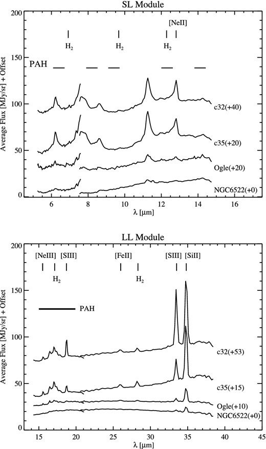
The (average) interstellar emission spectra for each of the fields. Note how the spectra reveal significant changes in the excitation conditions for the interstellar gas and dust for the different fields as one moves away from the Galactic Centre. Note that depending on telescope pointing accuracy, there can be mismatch between SL2/SL1, SL1/LL2 or LL2/LL1.
A first look at the variations in these interstellar spectra reveals different local excitation conditions. This can be inferred for example from the changes in the [S iii](33.5-μm)/[Si ii](34.8-μm) line flux ratio. At the same time, the characteristics of the PAH emission change quite dramatically, from very weak emission in NGC 6522 to very strong features (and pronounced 15–20-μm emission) when moving in closer to the Galactic Centre (GC). This suggests that most of the interstellar emission originates from material in the bulge itself, rather than from the ISM in the solar neighbourhood. An in-depth analysis of these interstellar spectra will be presented elsewhere.
5 STELLAR AND MOLECULAR CONTRIBUTIONS
The target spectra show a great variety in the appearance of spectral features; it is interesting to note that most spectra are dominated by features that are typically found in an oxygen-rich environment (e.g. H2O, SiO) while the typical carbon-rich species (e.g. HCN, C2H2, etc.) are not evidently present. Longwards of 10 μm, most of our spectra show various emission features originating from circumstellar dust (see Section 8.2). To obtain the pure dust emission spectra from these observations, we need good knowledge of the underlying emission and absorption characteristics from the AGB star and the surrounding warm molecular layers (see e.g. Tsuji et al. 1997; Cami 2002). For an AGB photosphere at the mid-IR wavelengths studied here, continuum opacity is dominated by H−, and in that case, the resulting IR continuum can be represented analytically by a modified blackbody function (Engelke 1992). However, many of these objects have significant amounts of water in their extended photospheres or in dense molecular layers. Since water has a near-continuous opacity in the mid-IR, the continuum is often effectively determined by these water layers. In addition, molecular features (most notably of SiO) can have a profound effect on the shape of the dust features, especially near 10 μm. Thus, a detailed inventory and discussion of the molecular content in these targets is appropriate. We will give particular attention to those targets that do not show obvious dust emission and are therefore ‘naked stars’. A good understanding of the properties of these objects will be of great help in obtaining the dust spectra for the other targets.
We point out here that some of our observations also reveal the clear imprint of interstellar extinction. This is most notable in the spectra of our naked stars as weak absorption around 10 μm. Extinction has the potential to dramatically affect our analysis of the resulting dust spectra since many minerals in the circumstellar environment of AGB stars also exhibit features around 10 μm. This greatly complicates our analysis. As will become clear, good knowledge of the molecular bands is helpful to quantify the effect of extinction (see Section 6), and is thus also facilitated by the study of our naked stars.
5.1 Molecular bands: inventory
Previous space-based missions have revealed that O-rich AGB stars are surrounded by warm layers that are rich in molecules. The most commonly detected molecules in the near-IR to mid-IR range are H2O, OH, CO, CO2, SiO and SO2 (see e.g. Cami et al. 1997; Justtanont et al. 1998; Ryde et al. 1998; Duari, Cherchneff & Willacy 1999; Yamamura et al. 1999a; Yamamura, de Jong & Cami 1999b; Jørgensen et al. 2001; Matsuura et al. 2002; Blommaert et al. 2005), and most of those are also prominently present in our Spitzer spectra (see Fig. 4). The only exception is CO since the fundamental of CO (at 4.6 μm) is not covered by IRS. At the resolution of our IRS spectra, detailed line profiles are somewhat smeared out, but the molecular bands often leave a noticeable and recognizable footprint in the spectra of our target stars.
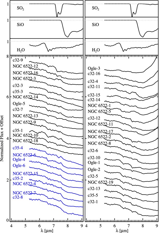
All our target spectra in the wavelength range 5–9 μm, showing the main molecular bands. The spectra are normalized to the flux at 6 μm, and are shown in order of increasing flux ratio at 10 to 6 μm (see Section 6, this ratio is taken from the fully corrected spectra and is the same as Fig. 15). Stars that we have classified as naked stars are shown in blue. For comparison, the top panel shows a few model spectra for the three most common molecular species (H2O, SiO and SO2).
The most important molecular component in these spectra is water vapour. In the wavelength range presented in Fig. 4, water reveals its presence by a fairly sharp drop in the flux near 6.5 μm corresponding to a strong increase in the water opacity. At longer wavelengths and at the low resolution of our observations, the variations in the water opacity can result in a broad emission-like feature centred around 10 μm (see Fig. 6) in pure water absorption spectra. A good characterization of the water absorption over the entire spectrum (but in particular under the 10-μm dust feature) is thus crucial for dust studies.
The SiO fundamental mode will also affect the dust spectra. SiO is a very abundant molecule in the atmospheres of AGB stars (Olofsson 2005). Models show that significant amounts of SiO are formed in stellar atmospheres with effective temperatures of ∼4000 K and less (Aringer et al. 2000). SiO is also a primary constituent for oxygen-rich dust and can be considered a prerequisite for dust production (Lebzelter & Posch 2001, and references therein). At the typical temperatures for the AGB atmospheres and molecular layers, SiO appears as a deep and broad absorption band with a clear band head at 7.55 μm, and with a red wing that can extend to 10–12 μm. SiO can therefore significantly alter the profile of dust features in the 10-μm region (see Fig. 4).
One molecular band that does not affect the dust spectrum much is the SO2 ν3 band at 7.3 μm. This band has been detected in the ISO/SWS spectra of some oxygen-rich AGB stars (Yamamura et al. 1999a), and can appear in absorption or in emission. Even at the low resolution of our observations, a close inspection of the spectra in Fig. 4 clearly shows the weak presence of this band in some of our targets – sometimes in absorption (e.g. NGC 6522-17) and sometimes in emission (e.g. c32-11). The SO2 band is relatively narrow and ends at about 7.7 μm, which is well before the onset of dust features. SO2 emission or absorption will thus not affect the resulting dust spectra much, but may make it harder to characterize the onset of the SiO band which is in the middle of the SO2 band.
Finally, we should note that our observations also include the wavelength range in which CO2 exhibits its bending mode around 15 μm, as well as several strong combination bands at 13.48, 13.87 and 16.18 μm that have been observed in O-rich AGB stars (Cami et al. 1997, 2000; Justtanont et al. 1998; Ryde, Eriksson & Gustafsson 1999; Markwick & Millar 2000; Woods et al. 2011). At the low resolution of our observations, these bands are not easily detected, but are nonetheless weakly present in some targets.
5.2 Molecular bands: models
It is clear from Fig. 4 that there is a considerable variation in the relative strengths and precise shapes of these molecular bands in our sample. Therefore, it does not seem adequate to use a single template spectrum as an approximation to the spectrum of the photosphere and the molecular layers, as is often necessarily done (e.g. Sloan & Price 1995) in similar studies. A better approach may be to use model spectra that reproduce the observed molecular bands shortwards of the onset of dust emission (∼ 8.5 μm), and predict the shape of the spectrum underlying the dust features. We investigate such an approach here.
For our purposes, we assume that the molecular layers are spherically symmetric, since only 1–6 per cent of Circumstellar Envelopes (CSEs) are estimated to be non-spherical among the entire population of single or binary AGB stars (Politano & Taam 2011). We then approximate this spherical geometry by plane-parallel slabs that are located in front of a background represented by an Engelke function (see Fig. 5) .
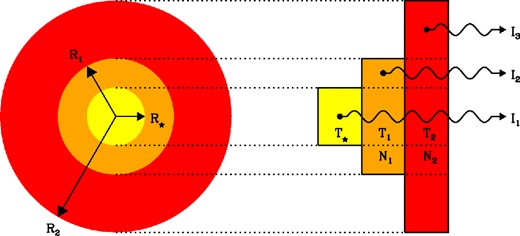
Illustration of how plane-parallel slab models can be used as an approximation to a spherical geometry when analysing the molecular bands around AGB stars. The leftmost slab (yellow) represents the stellar photosphere; the other two slabs are molecular layers characterized by their own temperature and column densities of contributing species. Radiative transfer is calculated along the three indicated rays. Changing the size of the layers changes the relative importance of emission to absorption. Figure taken from Cami (2012) (with permission).
Such models have been used successfully to reproduce mid-IR spectra of AGB stars (see e.g. Yamamura et al. 1999a,b; Cami et al. 2000; Cami 2002; Matsuura et al. 2002) and are computationally cheap. Water opacity plays a key role in our targets. It has been shown (Yamamura et al. 1999b; Cami 2002) that at least two layers containing water vapour are required to properly reproduce the observations, owing to the high opacity of water and temperature gradients in the photosphere and the circumstellar environment. We thus include two water layers in our models. We also added SiO to each of the layers. Each layer is then fully characterized by the temperature Tmol, the column densities N of water and SiO and the radius R; increasing the radius will result in a larger weight for the emission component (see e.g. Cami et al. 2000) and is required to reproduce emission features in the spectrum. Optical depths for each component are as described in SpectraFactory (Cami, van Malderen & Markwick 2010).
By changing the parameters of the slab model, we can reproduce a wide variety of infrared spectra. In its simplest form (with one slab only), the model already illustrates how a dense layer of water determines almost the entire mid-IR continuum (see Fig. 6). Indeed, if the water column density is high enough, the resulting spectrum is largely independent of the background flux due to the high water opacity over a large wavelength range. The main effect of such an opaque water layer is thus to lower the colour temperature of the apparent IR continuum (Cami 2002; Jones et al. 2002), but note also the appearance of a broad feature around 10 μm in these pure absorption spectra that could easily be misinterpreted as a dust emission feature (see Fig. 6).
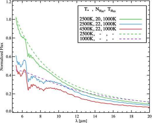
The infrared model spectra of three different slab models that only differ in their effective temperature and in the amounts of water. All models include a (T = 1000 K) layer of only water vapour. The green model represents pure absorption (I1 in Fig. 5) with only moderate amounts of water. This is the only model where the overall shape of the spectrum is similar to a blackbody at the object's effective temperature (in this case 2500 K, green dashed line). When only increasing the amount of water, we obtain the blue model. In this case, the shape of the spectrum looks more like a 1000-K blackbody (dashed purple line) – the temperature of the water layer. In the red model, we have changed the effective temperature but it looks almost identical (safe a scale factor) to the blue model: the water layer hides the stellar photosphere.
5.3 Modelling the naked stars
To get a feeling for the typical stellar and molecular parameters (i.e. temperatures, column densities and IR colour temperatures) corresponding to the infrared spectra of our AGB stars, we first apply our model to naked stars – stars that have no dust emission in their infrared spectra. However, the interplay of spectral features due to water, SiO and interstellar extinction makes it surprisingly hard to determine whether or not an object is a naked star by just visually inspecting the spectrum.
Here, we therefore adopt a slightly different working definition for a naked star. We will call a star in our sample a naked star, if its (extinction-corrected) IR spectrum can be well reproduced by our two-slab model containing water and SiO. This is not straightforward though, since extinction towards our targets is not well established, and an extinction-corrected IR spectrum is thus not easily obtained. In practice, we therefore included an extinction correction in our models (with the AK value as an additional model parameter). A naked star is then an object whose IR spectrum can be reproduced by our extinction-corrected two-slab model, provided that the best-fitting AK value is reasonable. Applying this approach to our entire sample, we found that out of 53 AGB stars in our sample only 9 of them qualify as naked stars since they result in reasonable AK values with acceptable fits. The implications for extinction are further discussed in Section 6.
In principle, our slab model has 10 free parameters: the temperature of the (Engelke) blackbody background (T⋆); for each of the two layers, a temperature Tmol, a size R, and column densities |$N_{\rm H_2O}$| and NSiO for water and SiO, respectively; and finally the extinction value AK. We imposed constraints on the temperature structure: the inner molecular layer cannot have a higher temperature than T⋆, and similarly the second layer cannot be warmer than the first layer. Since we do not see obvious emission features from cool molecular material, we did not include the third ray I3 that is being emitted from the second layer only. It is as though we set the second layer to be the same extent as the first layer. During a first run, we furthermore realized that all best-fitting solutions essentially had no detectable SiO in the second layer. We thus removed NSiO as a parameter in the second layer.
For each set of parameters, we first de-reddened the observed spectrum using the model AK value (see Section 6). We then created our model spectrum by calculating radiative transfer along each of the rays depicted in Fig. 5. Note that for our first run, we used all three rays, and for the final run only I1 and I2 (since R2 = R1). A full model spectrum is then obtained by summing a linear combination of these rays. We used a non-negative least-squares algorithm (see e.g. Lawson & Hanson 1974) to determine the scale factors that minimize the χ2 when comparing the final model spectrum to the observed (and de-reddened) spectrum. These scale factors really set R⋆ and R. Note that we only used the 6–14-μm wavelength range for calculating the χ2 value. Shortwards of 6 μm, there is potential contribution from the tail of a CO absorption band which is not included in our models. The longer wavelengths do not contain much in terms of distinct molecular spectral features. Therefore, by restricting ourselves to the SL (6–14-μm) modules, we avoid possible difficulties originating from a poor overlap between SL and LL modules. Finally, rather than calculating models for each grid point in the entire parameter space, we used an adaptive mesh algorithm that starts from a coarse grid covering the entire parameter space, and then reduces the step size at each iteration while centring the region of interest at the minimum in the χ2 hypersurface; the algorithm stops when all parameters have reached their desired step size and the χ2 minimum is centred in the region of interest.
We varied all parameters on a fixed grid except the layer size (R) which was left free and we determined by other means. Temperatures were changed in steps of 100 K. The background temperature T⋆ was set to vary between 2500 and 4500 K, and the temperature of the molecular layers Tmol between 500 and 2500 K (but subject to the constraints detailed above). We considered molecular column densities between N = 1016 and 1022 cm−2, and varied log N with a step size of 0.1. Finally, we varied the extinction value AK between 0 and 1 in steps of 0.01.
5.4 Modelling results
The nine naked star spectra and their best-fitting model are shown in Figs 7 and 8, and Table 2 lists the corresponding model parameters.1 Note that there is a considerable variation in the appearance of even these naked star spectra. In all cases, we can reproduce the observations reasonably well; in some cases though, there is some mismatch, most notably at the longer wavelengths corresponding to the LL1 module. While part of the discrepancy may point to remaining calibration issues, these clearly indicate shortcomings in our (simple) models, e.g. by producing too much water emission longwards of 20 μm in several objects.
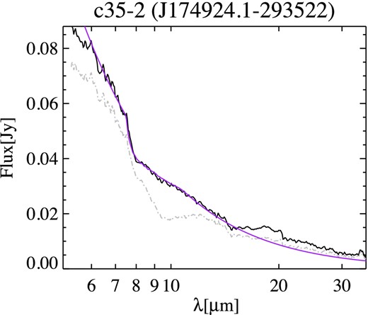
The raw Spitzer-IRS spectrum of c35-2 (grey), and the extinction-corrected spectrum (black) adopting a GC extinction law with AK = 0.49. The best-fitting model is shown in purple. Note the clear signature of interstellar extinction at 9.7 μm (silicate absorption) in the original spectrum.
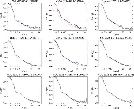
The nine naked star spectra and their best-fitting models. The original, uncorrected spectrum is shown in grey and the best-fitting extinction-corrected spectrum in black. The best-fitting stellar and molecular model spectrum is shown in purple.
The resulting best-fitting parameters for our naked star models and literature values for the extinction.
| Layer 1 | Layer 2 | ||||||||||||
|---|---|---|---|---|---|---|---|---|---|---|---|---|---|
| AK | T⋆ | R⋆ | T | |$\log (N_{{\rm H}_2{\rm O}})$| | log (NSiO) | T | |$\log (N_{{\rm H}_{\rm 2O}})$| | R/R⋆ | |||||
| (mag) | (K) | (×1013 cm) | (K) | (cm−2) | (cm−2) | (K) | (cm−2) | (R = R1 = R2) | |||||
| Object | a | b | c | d | e | ||||||||
| c32-8 | 0.51 | 0.78 | 0.43 | 0.52 | 4500 | 1.45 | 1800 | 17.4 | 22.0 | 1700 | 16.0 | 1.00 | |
| c35-2 | 0.54 | 0.87 | 0.43 | 0.54 | 2500 | 2.44 | 1600 | 16.0 | 22.0 | 500 | 16.0 | 1.00 | |
| c35-4 | 0.55 | 1.02 | 0.79 | 0.92 | 2500 | 2.88 | 1400 | 16.0 | 22.0 | 500 | 21.2 | 1.00 | |
| Ogle-4 | 0.30 | 0.26 | 0.06 | 0.25 | 2800 | 2.04 | 2000 | 16.0 | 22.0 | 500 | 16.0 | 1.00 | |
| Ogle-6 | 0.30 | 0.27 | 0.15 | 0.25 | 2800 | 2.58 | 1000 | 16.0 | 21.4 | 500 | 17.6 | 1.00 | |
| NGC 6522-4 | 0.18 | 0.17 | 0.15 | 0.27 | 3500 | 1.84 | 1900 | 16.0 | 22.0 | 500 | 16.0 | 1.00 | |
| NGC 6522-6 | 0.16 | 0.17 | 0.00 | 0.10 | 2500 | 2.33 | 1100 | 18.9 | 22.0 | 500 | 16.0 | 1.00 | |
| NGC 6522-7 | 0.06 | 0.15 | 0.07 | 0.14 | 4300 | 1.54 | 1000 | 16.0 | 22.0 | 600 | 18.9 | 1.00 | |
| NGC 6522-15 | 0.06 | 0.14 | 0.01 | 0.10 | 2500 | 2.31 | 1200 | 18.9 | 22.0 | 1100 | 16.0 | 1.00 | |
A key result from our modelling is that we do indeed find that in all cases, the spectra are best represented by models that include high column densities and high temperatures for SiO.
As can be seen from Table 2, our best-fitting models represent a fairly wide range of stellar temperatures T⋆ (2500 < T⋆ < 4500 K). However, we caution that these may not be well determined. As explained above and demonstrated in Fig. 6, the presence of water can significantly alter the shape (and corresponding colour temperature) of the IR continuum, and as a consequence, all information about the stellar continuum radiation is lost.
In few cases, we find that stars include a very thick water layer (e.g. c35-4); we must conclude that the stellar temperatures in those cases are ill-determined. Similarly, in those cases, the column densities for SiO are not well determined for the same reasons.
SiO is clearly present in our spectra and shows up most clearly at its band head at 7.55 μm. This indicates a high temperature, and from the depth of the band we can also infer that the column density must be high, but accurate values cannot be obtained for these objects with our simple models.
6 INTERSTELLAR EXTINCTION
Interstellar extinction can leave a significant spectral imprint especially in the 10-μm region where many minerals exhibit characteristic resonances. We selected our targets from fields covering the Galactic bulge that are typically characterized as having low extinction, and with most of the extinction originating from ‘local’ interstellar material rather than from regions within the bulge itself. However, we found that the effect of extinction on our target spectra is not negligible, and this is most easily ascertained by studying the naked stars. In several cases, this is clear and unambiguous from the appearance of an absorption feature around 9.7 μm in the spectra. The best examples are e.g. c35-2 and c35-4 (see Figs 7 and 8) where the spectra show the clear water absorption near 6.5 μm and the SiO band head near 7.55 μm that are typical for O-rich AGB stars, but in addition also exhibit a broad absorption band with the deepest absorption occurring near 9.7 μm. Clearly, this is not some other molecular absorption band, and the feature cannot be due to warm circumstellar dust either. Thus, interstellar extinction is clearly affecting our observations and needs to be corrected for. For other sources, the effect of extinction is more subtle and hard to establish visually.
Since interstellar extinction can also significantly affect the resulting dust spectra of our target AGB stars, we have taken great care in characterizing extinction in our different fields. We have done this by using the naked stars in our sample, and comparing different approaches to determine extinction in these lines of sight. We then use these results to estimate extinction for our remaining targets as well.
6.1 The IR extinction curve
The spectral shape of the extinction curve in the IR is discussed in great detail by Chiar & Tielens (2006). These authors construct two slightly different extinction laws: one that is appropriate for the ‘local’ ISM and another for the material towards the GC. Indeed, it is well known that the IR extinction towards the GC has a somewhat different shape than the extinction in the local ISM (Lutz et al. 1996); moreover, there is more silicate per unit of visual extinction towards the GC compared to the local ISM, resulting in a stronger 10-μm feature in the GC extinction curve. These extinction laws are consistent with earlier work by Lutz et al. (1996) and Indebetouw et al. (2005). On the other hand, Román-Zúñiga et al. (2007) found small differences with Chiar & Tielens (2006), indicating that the extinction law in the near- and mid-IR may vary slightly as a function of environment.
It is not clear a priori whether the extinction in the sightlines towards our targets is mainly due to dust in the local ISM or rather originates from material within the Galactic bulge, and we have thus considered both possibilities in this work. The extinction curves by Chiar & Tielens (2006) are presented as Aλ/AK (i.e. normalized to extinction in the K band) and cover the IR up to 27 μm. Since our spectra contain data up to 38 μm, we extrapolated the extinction curves to 38 μm by fitting a straight line longwards of 27.0 μm in the log–log plane of Aλ/AK versus λ, using the same slope as the extinction curve between 23 and 27 μm.
With the extinction curves expressed as Aλ/AK, we then still need a good estimate of the amount of extinction towards each of our targets (we will use AK here).
6.2 Literature AK values
The literature offers several extinction maps to estimate AK values based on the position of a target in the Galactic bulge. For our fields, especially the work by Schultheis et al. (1999) and Sumi (2004) are relevant. More recently, also Gonzalez et al. (2012) produced an extinction map for the Galactic bulge. The corresponding AK values for all three sources are listed in Table 2. Where necessary, we used the relations provided by Cardelli, Clayton & Mathis (1989) to obtain AK values.
It is clear from Table 2 that the most reddened targets are those in c32 and c35, and the least reddened field is NGC 6522 with the Ogle field intermediate between those two. However, there is considerable disagreement (up to a factor of 2.5) between these sources about the actual AK value for an individual target, and it is not clear which value is the best to use for our purposes. Thus, alternative ways are required to determine the extinction in our targets.
6.3 AK values from the slab models
Since the amount of extinction is in principle encoded in our observations, we also investigated how we could determine the AK values from the spectra themselves.
As described in Section 5, we included AK as a free parameter when modelling the naked stars. For each set of model parameters we considered, we furthermore compared the slab model to two different spectra: one where we applied the GC extinction curve and one where we applied the local ISM law. For all naked stars, we found much better overall model fits when using the GC extinction curve. Moreover, the resulting best-fitting AK values we obtain when using the GC extinction curve are generally better in agreement with some of the available literature values. Clearly, this indicates that for our purposes, the GC extinction law is more appropriate to use than the local ISM law. We have therefore adopted the GC extinction law from Chiar & Tielens (2006) for all targets in our sample.
When comparing the model AK values to the available literature values, we also find that the objects in c32 and c35 are subject to the most severe extinction, and that NGC 6522 is far less affected. However, for individual targets our derived value can be very close to either of the literature sources, or take on a very different value altogether. It is important to realize that the uncertainties on our derived AK values are significant though: there is a fairly large range in AK values around the best-fitting value over which the associated spectral changes can be accommodated by changing the properties of the molecular layers. Thus, also our models tell us that it is very difficult to disentangle the effect of low extinction from molecular features.
6.4 A model-independent approach
Finally, we tried to more directly determine the AK values from our observations without using models for the stellar and molecular contributions. The basic premise for this approach is fairly simple. Denoting with |$I_{\nu }^1$|, the specific intensity originating from a given naked star, and similarly using |$I_{\nu }^2$| to describe the intensity originating from a second naked star, the fluxes |$F_{\nu }^1$| and |$F_{\nu }^2$| that we observe from these stars scale with |$I_{\nu }^1{\rm e}^{-\tau _{\nu }^1}$| and |$I_{\nu }^2{\rm e}^{-\tau _{\nu }^2}$|, respectively, where |$\tau _{\nu }^1$| represents the optical depth of the interstellar material in the line of sight towards star 1 and |$\tau _{\nu }^2$| towards star 2. In Section 6.3, we investigate the two extinction laws (local and Galactic), and we verify that, between the two, the Galactic extinction law works better for all of our targets. We can write that |$\tau _{\nu }^1 = \tau _1 \tau _{\nu }$| and |$\tau _{\nu }^2 = \tau _2 \tau _{\nu }$|.
Fig. 9 shows an example of the resulting quotient spectrum after dividing two naked star spectra. In practice, the water signature in two different objects is not exactly the same, and some water residuals do show small-scale features as well as broad trends due to differences in IR colour temperature between the objects. Nonetheless, most water spectral features especially at the shorter wavelengths have disappeared. Other spectral features due to SiO and SO2 are confined to small wavelength ranges and easily recognized. What stands out most is the result of differential extinction between the two naked stars; as can be seen from the figure, the quotient spectrum closely resembles the Chiar & Tielens (2006) GC extinction law, especially around the 10-μm silicate absorption.
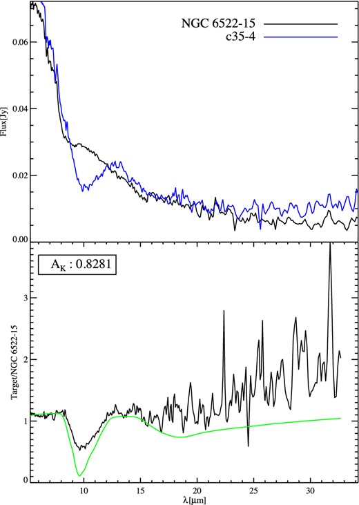
Top: the Spitzer-IRS spectrum of the reddened naked star c35-4 (blue) compared to the least reddened naked star NGC 6522-15 (black). Bottom: the result of dividing the spectrum of c35-4 by NGC 6522-15 (black). The green curve is the GC extinction curve by Chiar & Tielens (2006).
We then used this approach to determine AK values as follows. First, we determined that NGC 6522-15 is the naked star with the lowest amount of extinction. Indeed, when using this spectrum as a reference, all other naked stars show absorption in their quotient spectra at the wavelength of the interstellar silicate absorption feature. Therefore, all other naked stars must be subject to more interstellar extinction than NGC 6522-15. Note that this also agrees with the literature values by Schultheis et al. (1999) and Gonzalez et al. (2012).
For each of the remaining naked stars, we then created a set of extinction-corrected spectra, using |$A_K^\prime$| values (the ′ indicating that these may not reflect ‘true’ AK values) ranging from 0 to 1 mag in steps of 0.01, and we divided each corrected spectrum by the reference spectrum (NGC 6522-15). The resulting set of quotient spectra change in appearance from typically showing absorption near 9.7 μm (when undercorrected) to showing emission at the same wavelength (when overcorrected). A flat spectrum indicates a ‘perfect’ extinction correction. We quantified this by calculating the linear Pearson correlation coefficient between the quotient spectra and the Chiar & Tielens (2006) GC extinction curve in wavelengths between 8 μm and the maximum available wavelength in each case; correlation coefficients for our quotient spectra then typically change from positive values (for undercorrection) to negative values (overcorrection). We then simply determined the |$A_K^\prime$| value corresponding to a correlation coefficient of 0. In the process, we noticed that sometimes a strong SiO band can interfere somewhat with this process; we therefore used SiO model spectra (Cami et al. 2010) to divide out any SiO residuals before calculating the correlation coefficient.
Note that the procedure outlined above only determines the relative extinction between the target and the reference spectrum (NGC 6522-15) to the point where both spectra contain identical extinction spectral features. The actualAK value for the target is in principle given by |$A_K = A_K^\prime + A_{K}^{\rm NGC\,6522{\rm -}15}$|. To obtain AK values for our naked stars using the determined |$A_K^\prime$| values, we could simply adopt a set value for |$A_{K}^{\rm NGC\,6522{\rm -}15}$|. However, as is clear from Table 2, the literature offers quite different extinction values for this source. To reduce the sensitivity of our extinction values to a single source, we instead opted to calibrate our |$A_K^\prime$| sequence by using all available extinction values for all our naked stars (literature values as well as our own slab model results). We determined that setting |$A_{K}^{\rm NGC\,6522{\rm -}15}=0.10$| results in the lowest absolute deviation between AK values determined with this method and the weighted average of all other available values. Note that this value is within the uncertainty obtained using the Gonzalez et al. (2012) maps (who found |$A_{K}^{\rm NGC\,6522{\rm -}15}=0.14 \pm 0.09$|).
The resulting AK values for our naked stars are listed in Table 2; Fig. 10 shows a graphical comparison between the extinction values. In most cases, there is good agreement between these values and the results from our spectral modelling, and often, they are also close to one of the literature values. Since the AK values determined here are based on the individual spectra directly and are thus model independent, we deem them to be somewhat more reliable than the other values, and we thus adopt these AK values for the remainder of this paper.
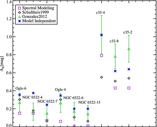
Extinction values (AK) for our naked stars from different sources and methods.
Armed with a good characterization of the extinction towards our naked stars, we can now better assess what extinction values to use for our dusty targets. Since the different fields have somewhat different extinction characteristics, it is insightful to evaluate our results per field. To furthermore get a feeling for the small-scale variability, it is also helpful to consider the Spitzer-Infrared Array Camera (IRAC) 8-μm images of our fields; these are taken from the GLIMPSE II survey (Churchwell et al. 2005) or from the work by Uttenthaler et al. (2010). The IRAC 8-μm images are particularly sensitive to the emission of PAHs in the 7.7-μm PAH band; these may thus give some information on the small-scale variability of interstellar dust. The details of this study are shown in Appendix B and the results are tabulated in Table 4 along with all other relevant extinction values.
A list of a few key features that characterize all our spectra and is sorted based on increasing mass-loss rate. Note that symbols such as ▵ and ◯ are used when the profile has a noticeable triangular or round appearance. In the cases where it is not easy to determine the actual shape of the profiles individually, we have used ✓ to denote the presence of the features. Note also that the actual peak wavelength of these features can be slightly variable throughout our sample (e.g. λpeak ∈ [9.7–10.3], [10.8–11.2], [12.8–13.2] μm).
| Identifier | λpeak ∼ 9.7 and 18 μm | λpeak ∼ 11 μm | λpeak ∼ 13 μm | λpeak ∼ 19.5 μm | λpeak ∼ 28.5 μm |
|---|---|---|---|---|---|
| NGC 6522-14 | ▵ | ✓ | ✓ | – | – |
| Ogle-5 | ✓ | ✓ | ✓ | – | – |
| NGC 6522-9 | ✓ | ✓ | ✓ | ✓ | – |
| c35-1 | ✓ | ✓ | ✓ | ✓ | – |
| NGC 6522-3 | ✓ | ✓ | ✓ | – | – |
| c32-3 | ✓ | – | ✓ | ✓ | – |
| NGC 6522-10 | ✓ | ✓ | ✓ | – | – |
| NGC 6522-16 | ✓ | ✓ | ✓ | ✓ | – |
| NGC 6522-12 | ✓ | ✓ | ✓ | ✓ | – |
| c35-3 | ✓ | ✓ | ✓ | – | – |
| c35-5 | ✓ | ✓ | ✓ | – | – |
| NGC 6522-13 | – | ✓ | ✓ | ✓ | – |
| NGC 6522-2 | ✓ | ✓ | ✓ | – | – |
| c32-7 | – | ✓ | ✓ | ✓ | – |
| c32-6 | ✓ | – | ✓ | ✓ | – |
| NGC 6522-19 | ✓ | ✓ | ✓ | – | – |
| c32-9 | ✓ | ✓ | ✓ | ✓ | – |
| c32-13 | ✓ | ✓ | ✓ | ✓ | – |
| NGC 6522-8 | ✓ | ✓ | ✓ | – | – |
| NGC 6522-17 | ✓ | ✓ | ✓ | – | – |
| c32-1 | ✓ | ✓ | ✓ | ✓ | – |
| Ogle-2 | ✓ | ✓ | ✓ | ✓ | – |
| Ogle-1 | ✓ | ✓ | ✓ | ✓ | – |
| c32-5 | ✓ | ✓ | ✓ | ✓ | – |
| c32-10 | ✓ | ✓ | ✓ | – | – |
| NGC 6522-5 | ✓ | ✓ | ✓ | ✓ | ✓ |
| NGC 6522-11 | ✓ | ✓ | ✓ | – | – |
| NGC 6522-1 | ✓ | ✓ | ✓ | ✓ | – |
| c32-12 | ✓ | ✓ | ✓ | – | – |
| c32-11 | ✓ | ✓ | ✓ | – | – |
| c32-14 | ✓ | ✓ | ✓ | ✓ | – |
| c32-15 | ✓ | ✓ | – | ✓ | – |
| c32-4 | ✓ | ✓ | – | ✓ | – |
| c32-16 | ◯ | – | – | – | – |
| Ogle-3 | ◯ | – | – | ✓ | – |
Extinction values for all our targets as well as SE classification. Note that naked stars (NS) do not belong to any SE class. The CC abbreviation refers to the method of using correlation coefficient.
| Identifier | AK (mag) | AK (mag) | AK (mag) | AK (mag) | AK (mag) | SE | log (L/L⊙) | |$\log {\dot{M}}[\mathrm{M}_{{\odot }}\,\mathrm{yr}^{-1}]$| | |$\log {\dot{M}}[\mathrm{M}_{{\odot }}\,\mathrm{yr}^{-1}]$| |
|---|---|---|---|---|---|---|---|---|---|
| (S99 and S04)a | (Modelling) | (G12)b | (CC) | (Final) | Index | (This work) | (Ojha et al. 2003) | ||
| c32-1 | 0.571 | 0.797 ± 0.136 | 0.581 | 5 | 4.02 | −6.97 | −6.03 | ||
| c32-3 | 0.518 | 0.772 ± 0.128 | 0.528 | 8 | 3.45 | −7.53 | −7.83 | ||
| c32-4 | 0.518 | 0.772 ± 0.128 | 0.528 | 7 | 4.08 | −6.55 | −5.30 | ||
| c32-5 | 0.507 | 0.780 ± 0.136 | 0.517 | 6 | 4.09 | −6.87 | −5.84 | ||
| c32-6 | 0.507 | 0.780 ± 0.136 | 0.517 | 8 | 3.91 | −7.06 | −6.90 | ||
| c32-7 | 0.507 | 0.781 ± 0.136 | 0.517 | 4 | 3.95 | −7.21 | −6.91 | ||
| c32-8 | 0.507 | 0.57 | 0.781 ± 0.136 | 0.518 | 0.520 | NS | |||
| c32-9 | 0.507 | 0.772 ± 0.130 | 0.517 | 5 | 3.93 | −7.06 | −5.62 | ||
| c32-10 | 0.507 | 0.743 ± 0.127 | 0.517 | 5 | 4.04 | −6.86 | −5.86 | ||
| c32-11 | 0.497 | 0.770 ± 0.133 | 0.507 | 6 | 3.97 | −6.66 | −5.79 | ||
| c32-12 | 0.528 | 0.781 ± 0.136 | 0.538 | 5 | 4.08 | −6.70 | −5.85 | ||
| c32-13 | 0.476 | 0.730 ± 0.135 | 0.486 | 6 | 3.84 | −7.01 | −6.36 | ||
| c32-14 | 0.507 | 0.775 ± 0.133 | 0.517 | 7 | 4.08 | −6.64 | −5.53 | ||
| c32-15 | 0.518 | 0.762 ± 0.142 | 0.528 | 7 | 4.02 | −6.56 | −5.55 | ||
| c32-16 | 0.550 | 0.790 ± 0.145 | 0.560 | 9 | 4.16 | −6.48 | −5.40 | ||
| c35-1 | 0.602 | 0.923 ± 0.169 | 0.600 | 6 | 3.42 | −7.60 | −6.90 | ||
| c35-2 | 0.539 | 0.49 | 0.865 ± 0.150 | 0.539 | 0.540 | NS | |||
| c35-3 | 0.624 | 1.033 ± 0.210 | 0.920 | 5 | 3.74 | −7.37 | −6.54 | ||
| c35-4 | 0.550 | 0.87 | 1.022 ± 0.212 | 0.920 | 0.920 | NS | |||
| c35-5 | 0.581 | 0.972 ± 0.217 | 0.920 | 7 | 3.56 | −7.34 | −6.39 | ||
| Ogle-1 | 0.302 | 0.252 ± 0.103 | 0.238 | 5 | 4.00 | −6.93 | −6.35 | ||
| Ogle-2 | 0.302 | 0.260 ± 0.107 | 0.242 | 5 | 3.97 | −6.95 | −6.54 | ||
| Ogle-3 | 0.302 | 0.260 ± 0.105 | 0.242 | 8 | 4.33 | −6.32 | −5.29 | ||
| Ogle-4 | 0.302 | 0.18 | 0.264 ± 0.105 | 0.246 | 0.246 | NS | |||
| Ogle-5 | 0.302 | 0.268 ± 0.104 | 0.254 | 6 | 3.22 | −7.66 | −9.18 | ||
| Ogle-6 | 0.302 | 0.21 | 0.268 ± 0.104 | 0.254 | 0.254 | NS | |||
| NGC 6522-1 | 0.127 | 0.171 ± 0.098 | 0.285 | 8 | 4.17 | −6.70 | −5.94 | ||
| NGC 6522-2 | 0.111 | 0.166 ± 0.097 | 0.275 | 5 | 3.50 | −7.22 | −6.93 | ||
| NGC 6522-3 | 0.155 | 0.152 ± 0.098 | 0.155 | 6 | 3.35 | −7.57 | −8.39 | ||
| NGC 6522-4 | 0.180 | 0.27 | 0.166 ± 0.097 | 0.275 | 0.275 | NS | |||
| NGC 6522-5 | 0.106 | 0.171 ± 0.097 | 0.100 | 6 | 3.70 | −6.84 | −6.39 | ||
| NGC 6522-6 | 0.160 | 0.10 | 0.171 ± 0.097 | 0.100 | 0.100 | NS | |||
| NGC 6522-7 | 0.063 | 0.18 | 0.150 ± 0.098 | 0.144 | 0.144 | NS | |||
| NGC 6522-8 | 0.090 | 0.148 ± 0.097 | 0.130 | 6 | 3.84 | −6.98 | −7.04 | ||
| NGC 6522-9 | 0.090 | 0.148 ± 0.097 | 0.130 | 7 | 3.35 | −7.63 | −8.58 | ||
| NGC 6522-10 | 0.106 | 0.143 ± 0.094 | 0.100 | 3 | 3.50 | −7.51 | −7.93 | ||
| NGC 6522-11 | 0.095 | 0.177 ± 0.098 | 0.100 | 7 | 4.09 | −6.77 | −7.03 | ||
| NGC 6522-12 | 0.063 | 0.147 ± 0.099 | 0.144 | 4 | 3.40 | −7.40 | −7.24 | ||
| NGC 6522-13 | 0.106 | 0.143 ± 0.094 | 0.100 | 3 | 3.80 | −7.33 | −6.85 | ||
| NGC 6522-14 | 0.085 | 0.143 ± 0.094 | 0.100 | 9 | 3.30 | −7.66 | −10.00 | ||
| NGC 6522-15 | 0.063 | 0.11 | 0.143 ± 0.094 | 0.100 | 0.100 | NS | |||
| NGC 6522–16 | 0.063 | 0.142 ± 0.096 | 0.100 | 4 | 3.35 | −7.49 | −7.91 | ||
| NGC 6522-17 | 0.085 | 0.143 ± 0.095 | 0.100 | 5 | 3.75 | −6.98 | −6.83 | ||
| NGC 6522-18 | 0.106 | 0.141 ± 0.098 | 0.12 | 0.157 | 5 | ||||
| NGC 6522-19 | 0.099 | 0.141 ± 0.098 | 0.12 | 6 | 3.79 | −7.06 | −7.29 |
7 THE FULL SPITZER-IRS SPECTRA
At this point, we have obtained the final Spitzer-IRS spectra for all targets in our sample, and we show these in Fig. 11. As we showed already in Fig. 4, the spectra are dominated, shortwards of 8 μm, by molecular features originating from the stellar photosphere and warm molecular layers. Circumstellar dust shows up quite clearly at longer wavelengths (most notably e.g. in the 10-μm emission complex), and there is a fairly large range in the amount of dust emission relative to the ‘naked star’ spectra in our sample. The OH/IR stars on top represent the most extreme cases where only dust emission (and self-absorption) is present.
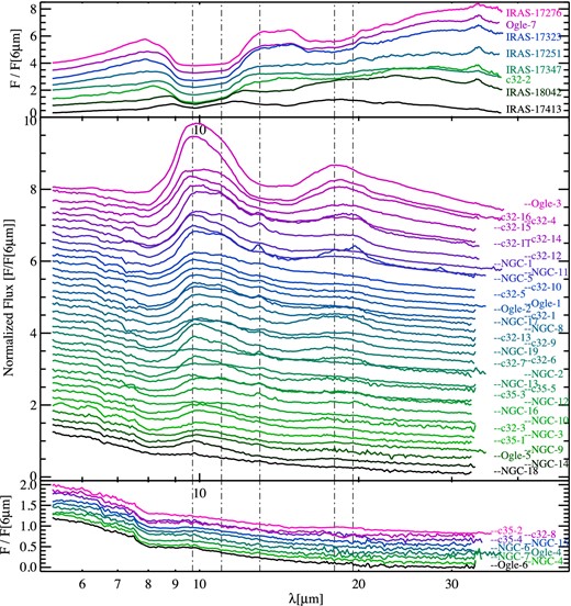
The full extinction-corrected Spitzer-IRS spectra of OH/IR stars (top), dusty targets (middle) and naked stars (bottom). The spectra at longer wavelengths are trimmed in the cases where data seemed too noisy and thus unreliable. The spectra are colour coded for better illustration. The spectra are normalized to their flux at 6 μm and are sorted as a function of increasing 10/6-μm flux ratio except for the dusty targets (middle) where the spectra are sorted as a function of increasing mass-loss rates (listed in Table 4). Shortwards of 9.7 μm, the molecular features are present with no clear trend; however, this figure represents a sequence of increasing dust optical depth (see the text for more details). Note that due to lack of space in this plot, we exceptionally used NGC as a short form of NGC 6522.
It is instructive to quantify the amount of dust and stellar emission and compare those to simple models for AGB stars with mass-loss. We therefore define Fmol as the integrated flux between 5 and 8 μm (where molecular bands are present, but no dust features) and Fdust as the integrated flux between 8 and 30 μm (the range with most conspicuous dust features and dust continuum). Note though that Fdust and Fmol both include a contribution from the stellar photosphere and molecular layers; at the same time, Fmol will not correspond to molecular bands for the optically thick OH/IR stars.
Fig. 12 shows how the integrated dust-free continuum flux Fmol changes as a function of the relative amount of dust emission (Fdust/Fmol) for the stars in our sample. In essence, this figure is similar to the CMD in Fig. 1, but it is derived purely from the Spitzer spectra. Compared to the naked stars (lower left of the diagram), our dusty targets follow a trend characterized by more dust emission (Fdust/Fmol) for higher stellar fluxes (Fmol), as was expected for our sample based on Fig. 1.
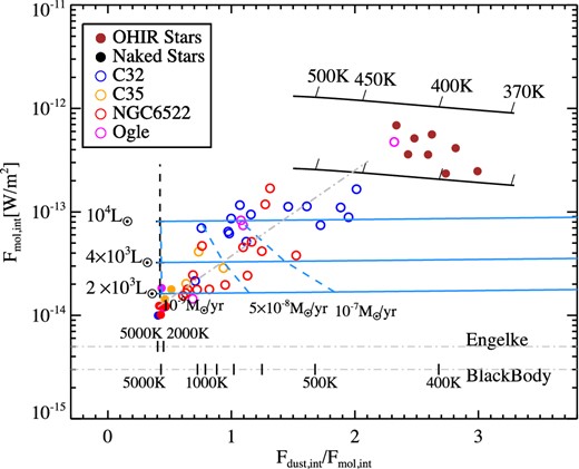
Fmol as a function of Fdust/Fmol for all objects in our sample. The black vertical dashed line on the left represents the locus for dust-free AGB stars for various luminosities at the distance of the Galactic bulge. The solid blue lines represent models for such AGB stars (at 2000, 6000 and 10,000 L⊙) surrounded by optically thin dust shells (of pure silicates) with increasing mass-loss rates; the blue dashed lines are lines of constant mass-loss rate (assuming a dust-to-gas ratio of 0.005). The solid black lines on top represent pure blackbody emitters at L = 2000 L⊙ (lower) and 10 000 L⊙ (upper) as an approximation of extremely optically thick dust shells. At the bottom, we have indicated the expected Fdust/Fmol values for, respectively, an Engelke function and for pure blackbodies with varying effective temperatures. The grey dash–dotted line is a least-absolute-deviation fit to the data points (excluding the OH/IR stars). See the text for details.
For comparison, we also show several models in Fig. 12. First, we indicate the locus for naked AGB stars at the distance of Galactic bulge (assumed to be 8.5 kpc). For this, we have used an Engelke function with an effective temperature of 3000 K for the stellar continuum and calculated Fmol and Fdust for luminosities between ∼2000 and ∼10 000 L⊙. This appears as the straight dashed line on the left side of the plot close to where naked stars are located. Note that changing the effective temperature (within reasonable limits for AGB stars) will primarily shift the line up or down.
We have also included a series of models for optically thin dust shells with increasing mass-loss rates, following the same approach as Schutte & Tielens (1989). All our models include only MgFeSiO4 silicate dust, i.e. olivine with equal iron and magnesium content (with optical constants from Dorschner et al. 1995); we have verified though that the results for other minerals are very similar. We calculated the emerging dust flux for total mass-loss rates ranging from 10−9 to 10−6 M⊙ yr−1 and assuming a dust-to-gas ratio of 0.005, as in Blommaert et al. (2006). We added this dust flux to the central stellar flux (for three different luminosities: L = 2000, 4000 and 10 000 L⊙). This results in nearly horizontal curves representing objects with the same stellar luminosities, but increasing mass-loss rates (and thus increasing dust emission).
As mass-loss rates increase, the dust will eventually become optically thick, and these models will not be applicable. An approximation for extremely optically thick dust shells (represented by the OH/IR stars) is shown in Fig. 12, where we have represented the optically thick dust shells by pure blackbody radiators of differing effective temperatures Tdust; two such curves are shown with luminosities of 2000 and 10 000 L⊙, respectively, that bracket the OH/IR stars in our sample. The downward trend for decreasing dust Tdust reflects that a smaller fraction of the dust emission is occurring in the 5–8-μm range; such a trend is also apparent in our OH/IR stars, whose decreasing dust colour temperatures can also be ascertained from Fig. 11.
The |$\dot{M}$| and L values are listed in Table 4. In Fig. 12, the lines that represent constant mass-loss rate (blue dashed lines) are nearly perpendicular to the best-fitting line. Additionally, increasing mass-loss rates at constant luminosities results in almost horizontal lines (blue solid lines), allowing every intersection with the best-fitting line to be traced back to its corresponding luminosity. Therefore, by projecting every data point on to the best-fitting line, we can estimate its corresponding luminosity which using equation (3) can lead to a rough estimate of the mass-loss rate.
Note that under several assumptions, this method is treated as a tool to estimate stellar luminosities and mass-loss rates directly from the Spitzer-IRS spectrum of an AGB star. These assumptions include modelling constraints such as stellar temperature, selective dust mineral, constant grain size, spherical grain shape and spherical symmetry in the outflow.
The location of our targets in this diagram compared to simple approximate models assures that our sample represents a sample of AGB stars at the distance of Galactic bulge, with increasing luminosities and mass-loss rates as we first envisioned, and is thus appropriate for studying the dust condensation sequence as a star climbs the AGB.
8 THE DUST SPECTRA
We now turn our attention to the dust. Here, we will only discuss a fairly basic characterization of the dust properties in our sample in terms of spectral components, and in terms of their classification following the well-known SE index (Sloan & Price 1995). Most of our discussion does not apply to the OH/IR stars, and we will therefore largely ignore them for the remainder of this paper. A much more detailed analysis will be presented in future papers.
8.1 Extracting the dust spectra
In order to study the spectroscopic properties of the dust alone, we need to be able to somehow separate the dust from the stellar (and molecular gas) component, and extract the pure dust spectra from the Spitzer observations. This, however, is not straightforward, and small errors on the stellar component can have an enormous impact on the dust spectra, especially for those targets with little dust emission.
An often used method to extract the dust spectra from IR AGB star spectra is to adopt a template spectrum for the underlying stellar contribution, scale to the observed spectrum at a key wavelength and subsequently subtract the template from the observed spectrum. The residual is then the dust spectrum. A widely used template in this context was discussed first by Sloan & Price (1995). These authors studied IRAS-LRS observations of five bright naked giants, and found that they could approximate these spectra starting from an Engelke function with an effective temperature of Teff = 3240 K. To this continuum, they added an SiO absorption band with a depth of 15 per cent, where the band profile was taken from the median absorption profile in their naked giants. The same template was then used for all O-rich AGB stars in their sample, and scaled to the observations by minimizing the χ2 over the wavelength range 7.67–8.58 μm.
It is clear form our work on the naked stars in Section 5 that a single template model cannot reliably reproduce all our naked stars. This already shows from the clear variations in the extinction-corrected spectra directly (see Fig. 8). When modelling these naked stars, we furthermore also used an Engelke function as the basis for our IR continuum, but we find very different effective temperatures than 3240 K (see Table 2); moreover, we found that the IR continuum is often dominated by the presence of an opaque water layer which lowers the IR colour temperature and produces broad features.
In Appendix D, we show how such a template compares to all of the dusty target spectra in our sample. In this case, the template is an Engelke function with Teff = 3240 K to which we have added a single SiO absorption layer (TSiO = 2000 K; NSiO = 1022 cm−2) such that the resulting SiO absorption band has a depth of 15 per cent. We scaled this template to the flux around 8 μm. For a few spectra (e.g. c32-1, c32-3), this template compares reasonably well to the observations at shorter wavelengths, but in most cases, the template only matches the observed spectrum near the wavelengths used for scaling and does not reproduce the stellar/molecular contribution at all – not in terms of the spectral features, but not even in terms of the shape of the continuum (e.g. c32-4 or Ogle-3). Moreover, any underlying spectral features due to water (which are often broad and present over the entire observed wavelength ranges) are not included in this template. It is thus not clear how reliable the extracted dust spectrum can be when adopting such a template, and it is worth it to consider some alternatives.
An appealing alternative would be to directly use some of the 10 naked star spectra as templates for the underlying stellar contribution. However, the large variations in the spectral features and continuum slope for the naked stars require some caution. We have tried such an approach by finding the naked star that contains the most similar spectral features to the dusty spectra in the 5–8-μm range. We then accounted for the continuum variations by first dividing out the naked star continuum (using a blackbody at the appropriate temperature) and multiplying the result by a blackbody of the appropriate temperature to match the dusty target. In some cases, this method works quite well; in others, there is much less correspondence. However, despite the obvious appeal in having an observed spectrum as the underlying template, this method has several drawbacks.
First and foremost, the existing noise in the naked star spectra will introduce significant noise to the extracted dust spectra (see Appendix D). Moreover, there is often a mismatch in the depth of SiO absorption feature between the two spectra that affects the onset wavelength of the resulting dust profile. Interestingly, we also found that in a few cases the strength of the resulting 13-μm feature is reduced since some of our template naked star spectra show an emission bump resembling that of a 13-μm feature (see Fig. 8). We have confirmed that this feature, unlike the small bump around 14 μm, is not introduced by discontinuities between the SL and LL modules. It is not clear though whether these weak bumps are instrumental artefacts or real spectral features (see Section 8.2.2 for further discussion).
Given these issues, we tried out yet another approach. Encouraged by our success in reproducing the 5–14-μm spectra of the naked stars with two-slab models in Section 5, we considered using the same models to fit each of our dust target spectra, by minimizing the χ2 in the dust-free wavelength range 5–8 μm, and then extending that model to the longer wavelengths. If this method works, it has the clear advantage that it provides a noise-free template for each target on an individual basis. However, this is a significantly smaller wavelength range, and thus it is not guaranteed that the results are representative for the full wavelength range.
To test the reliability of this approach, we determined the best-fitting model parameters for all our naked stars again, but this time only using the 6–8.5-μm range; we then constructed full spectra from the best-fitting parameters. In Fig. 13, we show how these models (6–8.5 μm) compare to the original best-fitting naked star models (6–14 μm). In general, both models are fairly similar. However, the only potential problem in using short wavelength range models (6–8.5 μm) is the under-representation of the naked star flux around 10 μm.
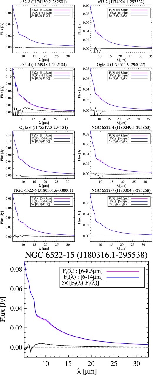
A comparison of different model spectra for the naked stars: models obtained from fitting the 6–14-μm range (blue) and from fitting only the 6–8.5-μm range (magenta). The two models are virtually indistinguishable between 6 and 8.5 μm, and in almost all cases, correspond to roughly the same stellar parameters. The black curve shows the residual difference between the two models. Note that the residuals are scaled (×5) for clarity.
Thus, by using models determined from fitting the 6–8.5-μm region as templates, there is a risk that we introduce artefacts in the resulting dust spectra. The shape of these artefacts is clear from Fig. 13: a fairly narrow emission feature around 9.5 μm (e.g. Ogle-6, NGC 6522-4), or alternatively a broad feature starting around 8 μm and sometimes extending up to 20 μm (e.g. c35-2, NGC 6522-7) or a combination of the two (e.g. NGC 6522-18). In the worst case (e.g. NGC 6522-18), these show up at a strength of about the 20 per cent of the stellar flux level but in other cases, these artefacts are not very prominent (typically ∼5 per cent of the flux).
Appendix D shows a comparison between the best-fitting 6–8.5-μm model and the template from Sloan & Price (1995) and the observed naked star templates, for all our targets. In most cases, the differences between the different approaches for the resulting dust spectra are negligible. The most pronounced differences occur on the blue edge of the 10-μm dust complex, and they are most pronounced for the objects with low amounts of dust emission (e.g. c35-1) or lowest stellar colour temperature (e.g. Ogle-3).
In conclusion, the modelling method amongst all provides a much better reproduction of the molecular features and the overall shape of the continuum. We thus adopted the modelling method to subtract the stellar and molecular contribution from the data, and to extract the dust spectra. It is clear though that there would be some benefit in having more reliable underlying template spectra for these objects.
8.2 A spectral inventory
The extracted dust spectra of all our targets are shown in Fig. 15 and reveal a diversity of spectral features. The dust composition (as traced by the spectral features) furthermore appears to be quite different for stars with low mass-loss rates (bottom) and high mass-loss rates (top). Table 3 provides a general description of a few key components by which we can characterize our entire sample. Note that the peak position of the features can be variable between the specified range as well as their overall shape. Some features are more round compared to some other that appear more triangularly shaped.
In the following, we offer a more detailed description of the spectral features and discuss the variations in our sample. To guide the eye in the following discussion, we show in Fig. 14 the particularly rich spectrum of NGC 6522-5, as well as dust scattering efficiencies for various minerals that we discuss here.
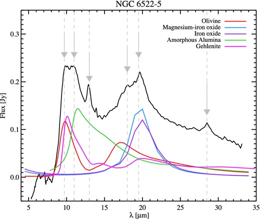
The dust spectrum of target NGC 6522-5 which seems to have a particularly rich variety of dust features; some of those are indicated with arrows. For comparison, we also show the dust scattering efficiencies for some minerals that have been proposed as carriers for these dust features: silicates (the olivine MgFeSiO4 is shown in red; Dorschner et al. 1995), gehlenite (Ca2Al2SiO7; magenta; Mutschke et al. 1998), alumina (Al2O3; Begemann et al. 1997), iron oxide (FeO; purple; Henning et al. 1995) and magnesiowüstite (MgFeO; blue; Henning et al. 1995).
8.2.1 The 10-μm region
All our targets exhibit clear dust emission around 10 μm. For the targets in the top part of Fig. 15, the 10-μm feature is smooth and roundish, and peaks at 9.7 μm – characteristic of amorphous silicates. The second emission band commonly associated with such minerals, at 18 μm, also appears quite clearly in those spectra. Thus, for the objects near the top, the dust emission is largely due to amorphous silicates. However, there are clear variations in the precise shape of the 10-μm emission feature even for those ‘silicate’ sources. For some targets, a shoulder appears at slightly longer wavelengths. As we further move down the sequence in Fig. 15, the character of the band changes significantly. In some sources, the 10-μm complex becomes much more sharply peaked (e.g. c32-6, c35-5, NGC 6522-14), and as we approach the bottom part of the figure, emission in this range looks very different from the smooth silicate profiles at the top. Clearly, the dust composition in those targets must be different.
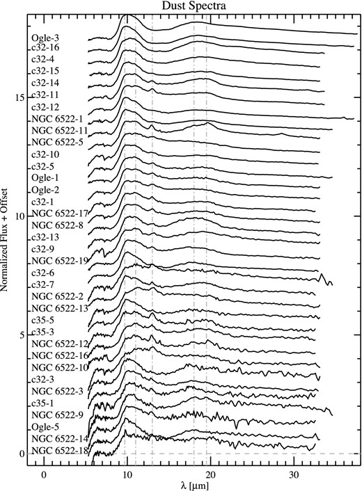
The final dust spectra sorted based on increasing mass-loss rate. Mass-loss rates are estimated using equation (3). Overall as we go from bottom to top, different features show noticeable variations in terms of strength, shape and peak wavelength (see the text for more details).
Differences in the dust composition as a function of mass-loss rate have been observed before for samples of nearby, bright AGB stars (e.g. Cami 2002; Heras & Hony 2005). However, for those samples, the targets with the lowest mass-loss rates show a first emission peak at 11 μm and an overall dust spectrum that resembles emission from alumina (Al2O3; see Fig. 14). This 11-μm feature had already been detected in Mira variables observed with the IRAS-LRS by Little-Marenin & Little (1990), who proposed crystalline olivine to be the carrier of this feature. Begemann et al. (1997) and Miyata et al. (2000) on the other hand related the 11-μm feature to amorphous alumina oxide grains. Cami (2002) shows, based on ISO-SWS spectra, that this feature peaks at 11.1 μm, while crystalline olivines peak at slightly longer wavelengths (11.3 μm), thus corroborating the assignment to amorphous alumina. In our sample that we present here though, there is not a single target where the emission peaks at 11 μm, or where the dust spectrum resembles pure alumina. However, many spectra show a clear emission bump at 11 μm, and this alumina may certainly be a contributing component.
There may be various other components that contribute to the 10-μm emission complex. Of particular interest in the studies of dust condensation are mellilites – a group of sorosilicates that are also commonly found in Ca and Al-rich inclusions in primitive chondrites. In meteorites, these mellilites form a solid solution between the Al-rich endmember called gehlenite (Ca2Al2SiO7) and the Mg endmember åkermanite (Ca2MgSi2O7). In their analysis and modelling of a sample of O-rich AGB stars, Heras & Hony (2005) found that including gehlenite significantly improved the quality of the resulting fit both in the 10- and 20-μm regions. Note that these authors used the optical constants from Mutschke et al. (1998).
Chihara, Koike & Tsuchiyama (2007) presented IR absorption spectra of the entire mellilite solid solution series between åkermanite and gehlenite. For all components, there are several peaks noticeable, including in the 9–13-μm region, but also at 14, 15, 17, 19, 21, 24, 30, 37 and 60 μm. In the 10-μm region, the gehlenite sample shows a spectrum that is quite different from Mutschke et al. (1998), and shows a broad flat-topped, trapezoidal 10-μm feature with several small peaks superposed. The pure åkermanite on the other hand shows a much narrower 10-μm profile with sharp and prominent peaks at 10.3, 10.7 and 11.7 μm. It is not clear how much these minerals could contribute to the spectra of our targets though; in addition to the 10-μm range, all mellilites also show strong features between 20 and 30 μm, where our spectra show little to no spectral structure.
8.2.2 The 13-μm feature – the first condensate?
Many, but not all, of our dust spectra also show the clear presence of the so-called 13-μm feature. Vardya et al. (1986) were the first to discover this feature when they studied IRAS-LRS spectra of about 20 Miras. They attributed the feature to some sort of silicate. The feature was later associated with oxygen-rich AGB stars (Sloan, Levan & Little-Marenin 1996). Recently, several candidates have been proposed to be the carrier of the 13-μm feature. The three main candidates are corundum (crystalline Al2O3), spinel (MgAl2O4) and silicon dioxide (SiO2; see DePew, Speck & Dijkstra 2006, and references therein). Recently, Zeidler, Posch & Mutschke (2013) measured the optical constants of some of these minerals, and favour oblate corundum grains as the carriers for the 13-μm feature.
In our sample, this feature is found in many of our targets. However, we also noticed that our naked stars Ogle-4 and NGC 6522-18 may exhibit this feature. The best example is Ogle-4, where a weak feature at 13 μm appears at about the 2.6σ level, with a width and profile similar to the 13-μm feature in our dusty targets (e.g. NGC 6522-5). If this is indeed the same 13-μm feature, it could indicate that the carrier of that feature is really the very first dust species to condense in the environment of O-rich AGB stars – maybe even in stars that otherwise produce no noticeable dust at all. Further confirmation of this detection would be desirable.
8.2.3 The band at 19.5 μm
A broad and sharply peaked feature at 19.5 μm (sometimes also called the 20-μm feature) is often seen in O-rich AGB stars. Little-Marenin & Little (1990) and Goebel, Bregman & Witteborn (1994) already detected and described it in their IRAS-LRS spectra. Following earlier work by Begemann et al. (1995), Henning et al. (1995) suggested that magnesium–iron oxides (magnesiowüstite) could indeed be responsible for the strong emission seen near 19 μm in some oxygen-rich stars that lack the broad silicate features. Indeed, laboratory spectroscopy of magnesium–iron oxides in the mid-IR shows a single absorption band in the 15–20-μm range; the precise peak wavelength shows a strong dependence on the Mg/Fe ratio: pure FeO peaks at 20 μm; as the Mg content increases, the peak shifts to shorter wavelengths. Observations with ISO-SWS yielded many more spectra of much higher quality; based on such observations, Cami (2002) and Posch et al. (2002) independently confirmed the good correspondence between the astronomical observations and laboratory spectra of Fe-rich MgFeO (Mg0.1Fe0.9O). A few more objects were discussed by Van Malderen (2003) and Heras & Hony (2005).
In our sample, there is far less evidence for the presence of this band. The 19-μm feature appears clearly in the spectrum of NGC 6522-5, but is not obviously present in the other targets; further analysis will have to confirm whether or not the band is possibly weakly present in other targets. For NGC 6522-5, the peak position is consistent with earlier studies, i.e. we find that the best correspondence with the laboratory measurements occurs for magnesiowüstite with a 10 per cent Mg fraction (Mg0.1Fe0.9O; Henning et al. 1995).
8.2.4 The band at 28.5 μm
We only observe the 28.5-μm feature in one of our sources (NGC 6522-5). On first sight, this feature may resemble enstatite; however, we have compared it to the feature that is identified as enstatite in Jones et al. (2012) and verified that they are not the same neither in terms of shape nor the peak wavelength. We have overplotted and investigated the dust scattering efficiency for enstatite and did not find a match there either. There is a possibility that this feature is due to a crystalline grain but its actual carrier is not yet fully confirmed.
8.3 Variations in the dust composition
In Fig. 15, we show the extracted dust spectra (normalized to the peak of the dust emission) sorted as a function of increasing mass-loss rate. These mass-loss rates were estimated from equation (3).
Compared to similar sequences obtained for nearby AGB stars (e.g. Cami 2002; Heras & Hony 2005), there are some similarities, but also very clear differences in the variations that we see in the dust spectra. Indeed, these studies showed a clear difference between objects with low mass-loss rates whose spectra are dominated by oxide-type dust (as seen through 11-, 13- and 19-μm features), and Mira variables with higher mass-loss rates whose spectra show primarily SE (broad and smooth 10- and 18-μm bands). Fig. 15 reveals a somewhat more chaotic picture for our target stars. The spectra of objects with high mass-loss rates (the top spectra in Fig. 15) show the broad SE bands, but there are no clear objects in our sample whose spectra are characteristic of the oxide-dominated dust. For instance, we see no single spectrum that is dominated by an alumina-like dust emission profile. Similarly, as noted above, the 19-μm band attributed to MgFeO is only clearly visible in one object (NGC 6522-5) which happens to have a fairly high mass-loss rate.
It is also interesting to note that the 13-μm feature appears in most of our spectra, although there seems to be no clear trend regarding the strength of this feature as a function of mass-loss rate. There are objects with both high and low mass-loss rates where the 13-μm feature is absent or very weak.
Thus, while our sample does show clear variations in the spectral content of our targets, these variations are not easy to interpret. It seems that spectra dominated by oxide dust are under-represented in our sample, and there is no clear one-to-one relation between mass-loss rates and dust composition as traced from the spectra.
8.4 The SE classification of our targets
Fig. 16 shows the SE classes for all targets in our sample. All targets cluster around the power-law line described by Sloan & Price (1995); however, it is immediately clear that class SE1 is absent and class SE2 is only represented by two targets, and in fact most of our targets are in classes SE5 or higher. This seems to confirm our conclusions from studying the dust spectra in Fig. 15 where we found that no target seems to correspond to a pure oxide dust spectrum.
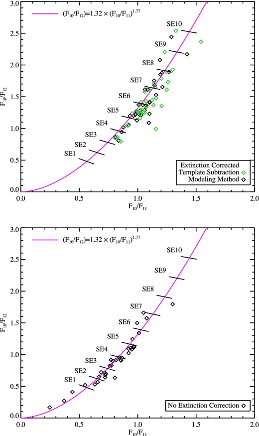
The SE classification for our sample after applying an extinction correction (top) and without applying an extinction correction (bottom). Flux ratios for our targets are indicated with the black diamonds; the green symbols indicate ratios obtained when using a similar stellar template as Sloan & Price (1995). The solid curve indicates the power law through the classes derived by Sloan & Price (1995) and the SE classes themselves are separated by grey lines (dashed and dotted for better illustration).
When we determined the SE classes, we used the dust spectra obtained by subtracting a detailed model of the underlying stellar and molecular contributions. This is different from Sloan & Price (1995) who used the same template model for all their objects (see Section 8.1). We have therefore repeated our classification, but this time using dust spectra obtained by subtracting the same template. While there are small differences in the resulting classification, those are details and the overall conclusion remains the same: the lower SE classes are missing or under-represented in our sample.
This result is somewhat surprising, given the goal of this programme and our careful sample selection. Either something must have gone wrong in the sample selection or, alternatively, our conclusions indicate that the dust around the AGB stars in the Galactic bulge might be somewhat different from the dust composition in the solar neighbourhood. It is clear though that a first contributing factor is certainly extinction. Indeed, at the time of our sample selection, reliable quantitative information about extinction towards our targets was scarce, and there was no reason to assume large variations in extinction values from one line of sight to another; our sample selection was thus based on sampling a CMD that was not corrected for extinction. The effect of extinction on our SE classification is illustrated in the bottom panel of Fig. 16, where we show the classes obtained without performing an extinction correction. In this case, we find a much more uniform coverage of the different SE classes. One could thus easily dismiss our ‘missing classes’ conclusions as due to these extinction effects and improper sample selection.
However, this cannot be the main or only reason for this effect. Indeed, it is important to realize here that we did select some of the bluest targets possible (see Fig. 2 and our discussion in Section 2); and even in the presence of extinction, this selection ensured that we have about nine naked stars in our sample. If extinction would systematically shift our targets to the higher SE classes, we should not have found any naked stars in our sample either.
Thus, we have to entertain the possibility that the absence of the SE classes represents a real effect, possibly due to different conditions in the Galactic bulge (e.g. lower metallicity). If proven correct, this could offer valuable insights into the dust condensation around O-rich AGB stars; follow-up work relating to this question will be the topic of further research.
9 SUMMARY AND CONCLUSIONS
We have obtained Spitzer-IRS spectra for a sample of AGB stars in the Galactic bulge with targets that were selected based on their (Ks − [15])0 colour in order to cover the full range of low to high mass-loss rates on the AGB. Strong and variable background emission in the crowded bulge fields complicates data reduction, and our targets suffer from interstellar extinction.
Using a subset of naked stars in our sample, we compared different methods to quantify and correct the interstellar extinction in our fields, and adopted extinction values derived from a model-independent analysis of the naked stars. From these naked star values, and from literature results as well as IRAC images, we estimated the extinction towards our dusty targets as well, and de-reddened our observations.
We constructed a Spitzer-IRS based CMD, and used this to estimate luminosities and mass-loss rates for our targets. With these, we can characterize our sample, and confirm that it indeed corresponds to AGB stars at the distance of the Galactic bulge (∼8.5 kpc) covering the entire range of mass-loss rates expected on the AGB. We modelled the underlying stellar and molecular spectral contributions between 5 and 8 μm, and used these results to construct the stellar and molecular model spectra over the entire Spitzer-IRS wavelength range; these models were then subtracted from the observations to obtain the dust spectra.
A first analysis of the dust spectra by carrying out a spectral inventory and by determining the SE classification for our targets shows that our sample shows clear variations in the dust composition, but these changes are not clearly related to changes in the mass-loss rates. Due to extinction, the lower SE classes (corresponding to spectra dominated by oxides) are somewhat under-represented in our sample. The detection of a 13-μm band in two of our naked stars entertains the possibility of this feature being among the first dust grains to condense out.
Further work on this sample of spectra will include detailed modelling of the spectra, studying the relation with metallicity and comparison with pulsational properties obtained from ground-based data.
SSG and JC acknowledge support from an NSERC Discovery Grant and a start-up grant from the Department of Physics and Astronomy at Western University. FK is being supported by grant NSC100-2112-M-001-023-MY3 from the National Science Council. This research has made use of the SIMBAD data base, operated at CDS, Strasbourg, France, and of NASA's Astrophysics Data System Bibliographic Services.
This work is based on observations made with the SpitzerSpace Telescope, which is operated by the Jet Propulsion Laboratory, California Institute of Technology under a contract with NASA. The IRS was a collaborative venture between Cornell University and Ball Aerospace Corporation funded by NASA through the Jet Propulsion Laboratory and Ames Research Centre. smart was developed by the IRS Team at Cornell University and is available through the Spitzer Science Centre at Caltech. This publication makes use of data products from the Two Micron All Sky Survey, which is a joint project of the University of Massachusetts and the Infrared Processing and Analysis Centre/California Institute of Technology, funded by the National Aeronautics and Space Administration and the National Science Foundation.
Note that we will discuss our results for the extinction values in Section 6.
Note that a difference of 0.01 mag in AK results in spectral changes of less than 0.5 per cent in the 10-μm region; this is generally negligible.
REFERENCES
10 APPENDIX A: BACKGROUND REMOVAL
We compared different methods for removing the background emission. A standard background subtraction method for IRS staring observations is to perform a nod-by-nod subtraction of the images. This method works well if the background emission does not change much over the spatial scales corresponding to the distance between the nod positions. This method often yields good results. However, clear residuals are sometimes present (especially in c32 and c35) because of the significant spatial variations of the background emission. Other problematic cases in which nod-by-nod subtraction proves ineffective are those observations where a contaminating source happens to be located near one of the nod positions.
The optimal extraction routine (Lebouteiller et al. 2010) in the smart data reduction package offers an appealing alternative. The programme can trace multiple sources in the slit simultaneously, while representing the background emission and its variations in the spatial direction by a polynomial. For well-behaving backgrounds, this method furthermore yields the best possible signal-to-noise ratio on the extracted spectrum. However, the method assumes that the spatial variations at different wavelengths can be described by the same background equation. We find that clear background residuals are present in the final spectra of those targets with strong background emission whose spatial variations are very wavelength dependent (such as shown in Fig. A1).
![Illustration of the strong background emission in our observations, and how this emission can vary significantly at small spatial scales (within the slit). Left: the CCD image of the IRS observation corresponding to target c35-5 (LL, Order 2, Nod 2). Wavelength decreases from bottom to top. The dashed lines indicate three different spatial positions within the slit; the target trace can be seen between the green and the blue dashed lines. Right: the background spectra corresponding to the spatial positions indicated on the image. All three show clear PAH emission between 16 and 18 μm as well as a strong [S iii] line at 18.7 μm. Note how the intensity of the [S iii] line increases from the left to the right, while the PAH emission weakens.](https://oup.silverchair-cdn.com/oup/backfile/Content_public/Journal/mnras/443/4/10.1093_mnras_stu1317/2/m_stu1317figa1.jpeg?Expires=1716404655&Signature=MHKthBvGbbxSB5qifTb2~mzwUvXBeGWd7Uyr2KqoM5Mh7ggVKizWaQ8rLWc5ixnli3RfRwb2nawmb80d-audRaHCUeC6ERHhD1KpJMwg22pXUkciSp2CRHQw2F1638pqsFrO-uC~R2fgeq1A2ONjT2eyYklvQzcHkGApoDpfx7VpHPNhfSlgFP5z8m4BUxA9xPO303t3l20ZTTO65AI3-I8o8x1Y1hci26k5Xtwrjmj-axmFqJ5Az5jWtVoyc~lIqTdypDf7na3eN-DTkJ5T5ztWd3whdeTM~WJ~YkywqkEUcZP6NCqgwhCWAMGzIF3ZETDuYDWx3GUqohpShAJ9jw__&Key-Pair-Id=APKAIE5G5CRDK6RD3PGA)
Illustration of the strong background emission in our observations, and how this emission can vary significantly at small spatial scales (within the slit). Left: the CCD image of the IRS observation corresponding to target c35-5 (LL, Order 2, Nod 2). Wavelength decreases from bottom to top. The dashed lines indicate three different spatial positions within the slit; the target trace can be seen between the green and the blue dashed lines. Right: the background spectra corresponding to the spatial positions indicated on the image. All three show clear PAH emission between 16 and 18 μm as well as a strong [S iii] line at 18.7 μm. Note how the intensity of the [S iii] line increases from the left to the right, while the PAH emission weakens.
As the third and final alternative, we created a two-dimensional model of the background emission by performing a least-absolute-deviation straight line fit to the background flux at each column in the raw images (i.e. roughly at each wavelength) independently, without taking into account the columns in which strong point sources are detected.
Additionally, we have visually looked for columns that contain weak sources and we masked them out manually. The use of the least-absolute-deviation method ensures that little weight is given to such potential outliers in comparison with the strong and variable background features present.
The resulting background map generally represents the spectral as well as the spatial variations of the background emission quite well. We then subtracted this model from the raw images. This method generally works well, and no obvious background residuals are found in the extracted spectra. Moreover, the background maps can be used to study interstellar infrared emission towards the Galactic bulge (see Section 4).
In the end, we extracted the background using either the smart's polynomial subtraction or the two-dimensional modelling (detailed description is provided in Appendix B).
11 APPENDIX B: AK VALUES
B1 c32
Fig. B1 shows the IRAC 8-μm image for our targets in c32. The interstellar PAH emission is clearly patchy and variable even on these scales, and there is also some variation in the literature extinction values (see Table 4). Schultheis et al. (1999) find that extinction values for our targets range from AK = 0.48 to 0.60 with a median of AK = 0.51; Gonzalez et al. (2012) on the other hand find a range AK = 0.73-0.84 with the median at AK = 0.78. The variations in AK furthermore appear to correspond qualitatively with the intensity of the PAH emission in the images: extinction is lowest (at AK = 0.48 when using the Schultheis values) for c32-13 (left off centre) where little PAH emission is apparent; it is somewhat higher for most of the targets to the right (e.g. c32-10, AK = 0.51), but clearly higher in regions with stronger 8-μm emission (e.g. c32-16 on the left, AK = 0.55; c32-2 on the right, AK = 0.60). It is not a one-to-one correspondence though; for example, one would expect c32-14 and nearby c32-16 to have comparable extinction, but they are listed with AK = 0.51 and 0.55, respectively. Similar trends are also apparent in the values from Gonzalez et al. (2012), albeit with some subtle differences, and at much higher AK values.
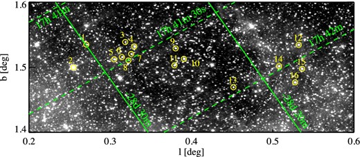
Unfortunately, we have only one naked star in this field (the object c32-8). Our best-fitting naked star model for this object corresponds to AK = 0.57, and our more robust model-independent method yields AK = 0.52 – very close to the AK = 0.51 value found by Schultheis et al. (1999) and much lower than the Gonzalez et al. (2012) value (AK = 0.78) for this object. It thus seems that the Schultheis et al. (1999) values are better for our targets. Since Schultheis et al. (1999) and Gonzalez et al. (2012) find roughly the same range in AK for our targets and roughly the same trends, our results indicate that for all targets in c32, we should use the Schultheis et al. (1999) values. For consistency with our model-independent values though, we have added 0.01 to each of the Schultheis et al. (1999) values2 (see Table 4).
B2 c35
Five of our targets are located in the field c35, and also for this field, there are clear variations in both the literature AK values and the 8-μm emission (see Fig. B2). However, for this field there is no clear correspondence between the two. Our targets are spatially clustered in two different locations (see Fig. B2). The first group contains dust target c35-1 and naked star c35-2. For the latter, we determined that AK = 0.54 using our model-independent method, in excellent agreement with Schultheis et al. (1999) but much lower than the AK = 0.87 value from Gonzalez et al. (2012).
It is clear from the extinction-corrected spectra and also from our naked star models that the AK = 0.87 value is far too high and results in a large overcorrection, while the AK = 0.54 value does not and furthermore results in good model fits as well (see Fig. B3), and we thus adopt this value for c35-2. Rather than using the same value for nearby target c35-1, we note that both Schultheis et al. (1999) and Gonzalez et al. (2012) agree that the AK value for c35-1 is roughly 0.06 mag larger than those for c35-2; we thus adopt the AK = 0.60 value for c35-1 as was done by Schultheis et al. (1999) as well.
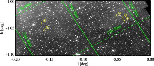
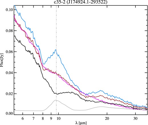
The best-fitting model for target c35-2 using AK values of 0.54 (model-independent, shown in brown) and 0.86 (Gonzalez et al. 2012, shown in black). The green shows the raw spectrum without extinction correction and the GC extinction curve is also overplotted in grey. The best-fitting models are overplotted in blue (for AK = 0.87) and magenta (for AK = 0.54).
The second group contains three objects that are close to each other, in what appears to be the same patch of 8-μm emission. For naked star c35-4, our model-independent method this time yields AK = 0.92, somewhat lower than the AK = 1.02 value found in Gonzalez et al. (2012) and significantly higher than the Schultheis et al. (1999) value of AK = 0.55. Indeed, using AK = 0.55 appears to undercorrect the spectrum in the interstellar 9.7-μm silicate feature (see Fig. B4), and we thus adopt AK = 0.92 as the proper value for c35-4. It is not clear though what to adopt for c35-3 and c35-5. While both Schultheis et al. (1999) and Gonzalez et al. (2012) find difference of about ΔAK ≈ 0.06 mag between the three objects, they disagree about which objects are most and least subject to extinction. Since this target is close to c35-3 and c35-5, and from the IRAC image, there is no clear change in the 8-μm emission between the three targets, we have applied the same AK value to them as well.
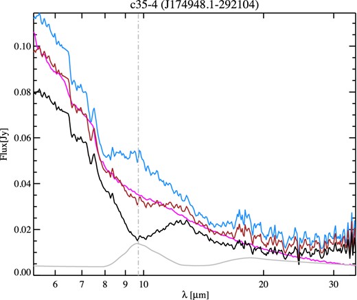
The raw spectrum of target c35-4 (in black) corrected for AK = 0.55 from Schultheis et al. (1999; in brown) and its corresponding best-fitting model (in magenta) and corrected spectrum using AK = 0.92 from the model-independent method (in blue). The GC extinction curve is also overplotted in grey.
B3 Ogle
Fig. B5 shows the IRAC 8-μm image covering our targets in the Ogle field. There is considerably less extinction towards our targets in the Ogle field than towards c32 or c35, and although the 8-μm image shows some variations in the 8-μm emission, extinction in this region is fairly homogeneous: for all our targets in the Ogle field, Sumi (2004) obtains a value of AK = 0.302 while Gonzalez et al. (2012) find a range between AK = 0.25 and 0.27.
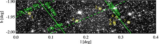
Ogle-4 and Ogle-6 are the two naked stars in this field. Unlike the naked stars in c32 and c35, the spectra for Ogle-4 and Ogle-6 do not reveal any obvious absorption feature near 9.7-μm at all; thus, these targets offer a clear example of the ambiguity in determining the interstellar extinction. We can in fact reproduce these spectra quite well (|$\chi ^2_{\nu }$| = 0.69 and 0.55, respectively) with our slab models without even applying an extinction correction (see Fig. B6) .
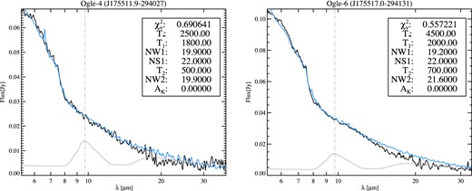
This figure shows the best-fitting models for Ogle-4 (left) and Ogle-6 (right) when no extinction correction is applied at all (i.e. AK = 0).
Using Gonzalez et al. (2012) maps, we find AK values of 0.264 ± 0.105 and 0.268 ± 0.104, and using the model-independent method, we find 0.246 and 0.254 for Ogle-4 and Ogle-6, respectively.
The Gonzalez et al. (2012) values show a marginal but consistent increasing trend in AK (∼ 0.05) between those targets in the field that have longitude difference of roughly ∼1°. This change will not affect the final spectra significantly but for consistency we have applied this trend to the targets of this field.
B4 NGC 6522
Extinction in NGC 6522 is lower than the Ogle field, but with considerable variations – literature values range from AK = 0.06 to 0.18 with a mean value of AK = 0.10 for our targets in this field. Also the 8-μm emission shows significant variations across the field (see Fig. B7). From Gonzalez et al. (2012) maps, we find a range from AK = 0.14 to 0.17 with a mean value of AK = 0.15.
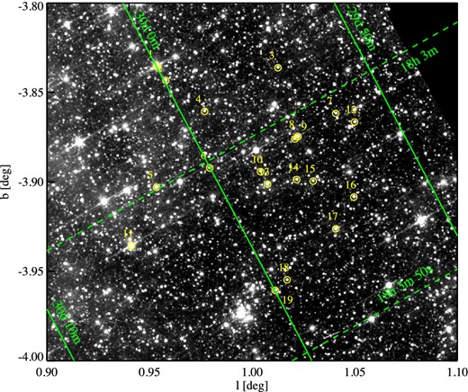
Targets NGC 6522-15 to NGC 6522-18 are all naked stars in this field. We have chosen the model-independent values as final values for all naked stars. It is not immediately clear whether or not there is an overall trend between the AK values of the targets in this field. In what follows, we attempt to find local trends.
It appears from Gonzalez et al. (2012) maps that targets NGC 6522-13, NGC 6522-17, NGC 6522-10, NGC 6522-14 and NGC 6522-16 have exactly the same value as NGC 6522-15. It is also clear from the IRAC image (Fig. B7) that in the region in which this group of targets are located, the 8-μm emission is not significantly variable and patchy. Our model-independent method yields the value of 0.10 for NGC 6522-15 which indicates that the Schultheis et al. (1999) value of 0.063 is an underestimation for this region. We thus apply the value of 0.10 to this group of targets.
Targets NGC 6522-8 and NGC 6522-9 have exactly the same AK value which according to both papers is slightly higher (∼ 0.03) than that of NGC 6522-15. Thus, for these two, we have added 0.03 to |$A_K^{{\rm NGC}\,6522{\rm -}15}=0.10$|.
Targets NGC 6522-7 and NGC 6522-12 are fairly close to one another, and the literature values suggest equal values for both. NGC 6522-7 is a naked star for which we found AK = 0.144 from the model-independent method. This indicates that similar to NGC 6522-15, the value of 0.063 listed by Schultheis et al. (1999) is an underestimation for this region. We used AK = 0.144 for these two targets.
The model-independent value for the naked star NGC 6522-6 yields 0.10 which points to an overestimation by 0.07 mag in both literature values. Target NGC 6522-5 is located in the same region as NGC 6522-6 with exactly the same AK value according to Gonzalez et al. (2012). However, Schultheis et al. (1999) estimate AK = 0.106 for NGC 6522-5 which is much closer to the value we find for this neighbourhood through our model-independent method. Therefore, we concluded that AK = 0.171 which was estimated from Gonzalez et al. (2012) maps is an overestimation for both NGC 6522-5 and NGC 6522-6, instead we used AK = 0.10 for both.
In the case of target NGC 6522-2, the closest naked star is NGC 6522-4 which has exactly the same AK from Gonzalez et al. (2012) maps but different values from Schultheis et al. (1999). Our model-independent value for NGC 6522-4 is 0.275, and it shows a clear underestimation in both literature values by roughly 0.1 mag. Our modelled value for NGC 6522-4 is 0.27 which also points to the underestimation in this region by both papers. Since the IRAC image does not show a clear and significant difference in 8-μm emission between NGC 6522-4 and NGC 6522-2 and also because Gonzalez et al. (2012) maps estimate exactly the same values for both of them, we have used AK = 0.275 for both of them.
Targets NGC 6522-1 and NGC 6522-2 are located fairly nearby; therefore, we can assume that this underestimation holds true for NGC 6522-1 as well. However, both literature values for NGC 6522-1 estimate a value which is higher than NGC 6522-2 by roughly 0.01mag. Therefore, for NGC 6522-1 we added 0.01mag to |$A_K^{{\rm NGC}\,6522-2}$| and used 0.285.
Target NGC 6522-3 has two literature values of AK = 0.152 ± 0.098 and 0.155 which are in reasonable agreement with each other. We have used an average value of AK = 0.153 for this target. This target stands fairly alone in the field; thus, it is not possible to use any other target to re-examine the AK value for NGC 6522-3 accordingly.
Gonzalez et al. (2012) maps estimate the highest AK value (0.177) for target NGC 6522-11 which is still not too different from that of NGC 6522-5 which is the closest target to it. We discussed that AK in the region of NGC 6522-5 was overestimated by Gonzalez et al. (2012) and that Schultheis et al. (1999) values are better representation of the correct extinction in these regions. It is not likely for extinction to change from 0.10 around NGC 6522-5 to 0.177 around NGC 6522-11 since any such dramatic change would have appeared clearly on the 8-μm IRAC image shown in Fig. B7. Therefore, we used AK = 0.1 for NGC 6522-11 as well. The final extinction values are listed in Table 4.
Targets NGC 6522-18 and NGC 6522-19 have similar AK values according to both papers. In Fig. B7, they are located in a fairly isolated region in the field. For these two targets, we took the average literature value of AK = 0.12 which is the same for both.
12 APPENDIX C
In this appendix, we present the final Spitzer-IRS spectra for our sample. In the text, we discuss the general data reduction recipe that was applied to all the targets. However, in few exceptional cases, slight modification to the general recipe was necessary. Here, we provide a brief per-target recipe that will allow the reader to achieve identical results.
Fig. C1 shows the extracted spectrum of each target. Note that the first and the second nods and modules are distinguished by a certain colour as shown in Table C1.
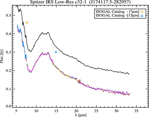
(c32-1) Both nods of the short low modules (SL1 and SL2) of this target contain only one target in the slit whereas in the long low module (LL1 and LL2) a second source appears very close to c32-1 (see Fig. C2). The positions of the extracted sources are shown in Fig. C2. The spectrum shows residuals from insufficient bad pixel removal around 20.5 μm which was properly masked. The background of this source is strong and variable with prominent PAH features. However, it can be properly modelled and corrected using the idl program discussed in the text. In the obtained spectrum, there is a slight mismatch between LL and SL modules. We treated this mismatch by scaling the LL modules with respect to the SL modules. The scaling factors used are listed below.
Colours used for each nod and module.
| Module | Nod | Colour |
|---|---|---|
| SL1 | First | Lime-green |
| SL1 | Second | Magenta |
| SL2 | First | Red |
| SL2 | Second | Sky blue |
| LL1 | First | Brown |
| LL1 | Second | Purple |
| LL2 | First | Dark blue |
| LL2 | Second | Orange |
| Module | Nod | Colour |
|---|---|---|
| SL1 | First | Lime-green |
| SL1 | Second | Magenta |
| SL2 | First | Red |
| SL2 | Second | Sky blue |
| LL1 | First | Brown |
| LL1 | Second | Purple |
| LL2 | First | Dark blue |
| LL2 | Second | Orange |
In Fig. C2, we show the point spread functions for each nod and module after correction for the background. The observed point spread function is shown in black, and our best-fitting point spread functions are shown in different colours depending on the number of sources detected in each of them. The caption of each figure shows the nod and module and its corresponding scale factor.
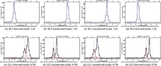
SL and LL modules spatial profiles after subtraction of the background.
In most of our targets after extraction, there still appears a residual from insufficient bad pixel removal in the form of unrealistic features (e.g. around 19.5 or 20.5 μm). We have manually removed those features by masking (removing from the flux array) those points from our spectra. The two nods within each module have been scaled to their common median in all of our targets.
The photometry data from ISOGAL (7, 15 μm), IRAC (3.6, 4.5, 5.8, 8 μm) and the Multiband Imaging Photometer (MIPS) (24 μm) are also overplotted. In most cases, the flux values we extract are in good agreement with the photometry values.
However, in some cases there appears to be a mismatch between the two. We do not have a clear reason that can explain these discrepancies in all targets. These occasional differences can be introduced by a combination of error sources (e.g. instrumental, data processing, variability, etc.). The intrinsic variability of the star over time might be a plausible contributing factor to the discrepancies.
In the whole sample (except of OH/IR stars), we chose SL1 to be our reference module because it has the most reliable and the least noisy flux compared to other modules. We have also tried using other modules as references as well, but in some cases it alleviates and in some other cases it aggravates the discrepancies. The scale factors applied on the LL modules range between ∼ 0.11 and 0.97 and for SL2 they range between ∼0.85 and 1.5. The typical offset between photometric data and spectroscopic data ranges between ∼0 and 2 Jy in flux. Fig. C1 shows one example of our targets. The full appendix is available online.
13 APPENDIX D
In this appendix, we present different extraction methods used to obtain the dust spectrum (see Section 8.1).
In Figs D1 through D7, the normalized spectrum of the dusty target is shown in black, the 5–8-μm range model for the dusty spectrum is shown in green, the scaled naked star that has the most similar features in 5–8 μm is shown in purple, and the template model used by Sloan & Price (1995) is overplotted in orange including a plain Engelke function at T = 3240 K (dashed blue line) to separate the continuum from the SiO absorption. In addition, the inset plots show the dust spectra that are obtained using each of these methods. The colour of each resulting dust spectrum corresponds to the particular method of extraction.
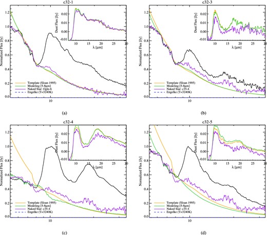
Different dust extraction methods for naked stars c32-1, c32-3, c32-4 and c32-5. See the text for more details.
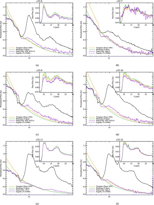
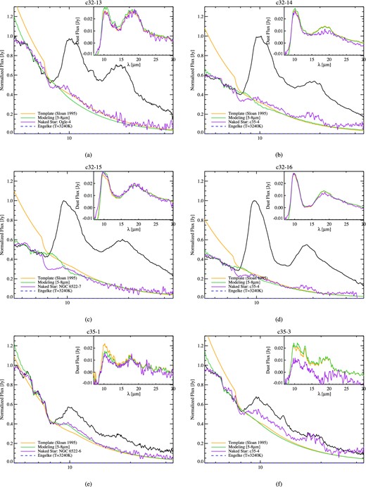
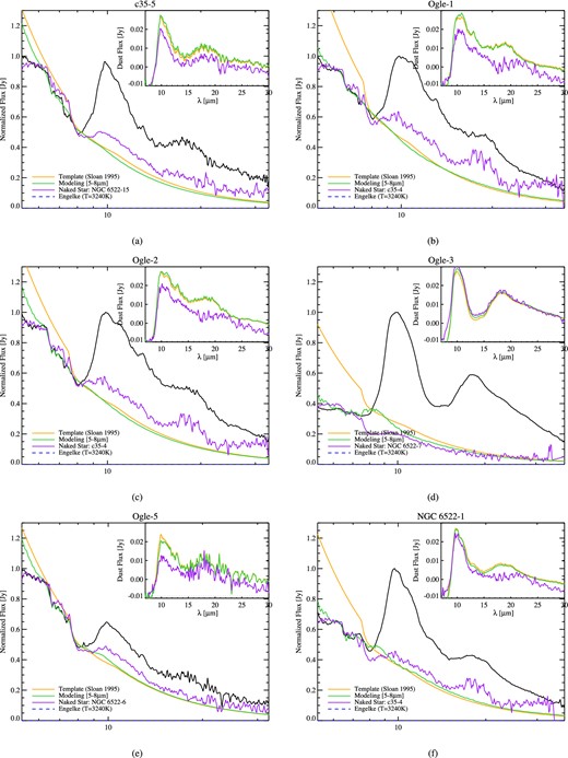

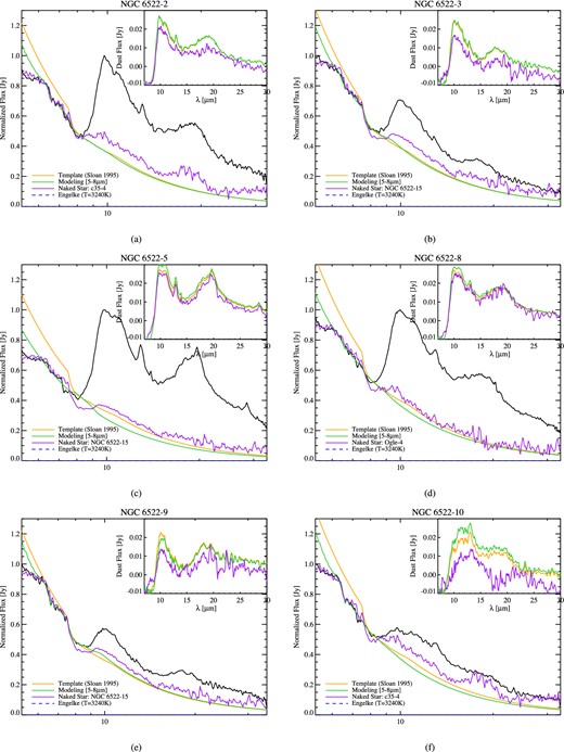
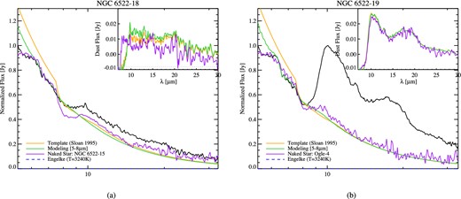
SUPPORTING INFORMATION
Additional Supporting Information may be found in the online version of this article:
Appendix C (Supplementary Data).
Please note: Oxford University Press is not responsible for the content or functionality of any supporting materials supplied by the authors. Any queries (other than missing material) should be directed to the corresponding author for the paper.
