

Abstract
The West African Sahel has been facing for more than 30 years an increase in extreme rainfall with strong socio-economic impacts. This situation challenges decision-makers to define adaptation strategies in a rapidly changing climate. The present study proposes (i) a quantitative characterization of the trends in extreme rainfall at the regional scale, (ii) the translation of the trends into metrics that can be used by hydrological risk managers, (iii) elements for understanding the link between the climatology of extreme and mean rainfall. Based on a regional non-stationary statistical model applied to in-situ daily rainfall data over the period 1983–2015, we show that the region-wide increasing trend in extreme rainfall is highly significant. The change in extreme value distribution reflects an increase in both the mean and variability, producing a 5%/decade increase in extreme rainfall intensity whatever the return period. The statistical framework provides operational elements for revising the design methods of hydraulic structures which most often assume a stationary climate. Finally, the study shows that the increase in annual maxima of daily rainfall is more attributable to stronger storm intensities (80%) than to more frequent storm occurrences (20%), reflecting a major rainfall regime shift in comparison to those observed in the region since 1950.
Export citation and abstract BibTeX RIS

Original content from this work may be used under the terms of the Creative Commons Attribution 4.0 license. Any further distribution of this work must maintain attribution to the author(s) and the title of the work, journal citation and DOI.
1. Introduction
Among the various implications of human-induced climate change, the high-impact weather events related to water are of special concern (Douville et al 2021). This prompted IPCC WG1 to devote a specific chapter to extreme events, with an emphasis on the regional scale (Seneviratne et al 2021). While acknowledging significant advances in the AR6 report, Seneviratne et al (2021) underline the important gaps that remain in our knowledge of how the rainfall extremes are evolving and will evolve at regional to sub-regional scales. At the same time, because current mitigation efforts are not sufficient to prevent large increases in temperature (Rogelj et al 2016, UNEP 2021), adaptation to new regional climates is becoming a central issue (Hulme 2020). Detection, attribution and projection are the three pillars of adaptation policies. Detecting already occurring changes is needed for guiding present adaptation policies. Attribution of these changes is the foundation for reliable projections, needed to anticipate how present adaptation policies might have to evolve in the future, depending on various scenarios of anthropogenic forcing. Detection is a matter of signal-to-noise ratio, any speculated evolution of a climate parameter being embedded in the internal climate variability (see e.g. Hegerl et al 2015). This signal is notoriously weak for rainfall due to its intermittent nature, making detection especially difficult and requiring long-term, accurate and homogeneous observational series that only ground-based networks can provide. This paper is addressing this detection issue for the ongoing evolution of extreme rainfall in the West African Sahel.
Dry or semi-arid tropical regions such as the Sahel are characterized by a strong interannual and decadal rainfall variability (e.g. Nicholson 2013, Biasutti 2019) and thus a noisy natural signal. Theory (O'Gorman and Schneider 2009, Trenberth 2011) and models (Sillmann et al 2013, Fischer and Knutti 2016) point to global warming causing longer dry spells and stronger storms. In the Sahel, the raw analysis of observations seems to establish that an increasing trend in extreme rainfall is already effective (Panthou et al 2014, 2018, Taylor et al 2017). However, it remains to infer how robust this trend detection is at regional scale i.e to quantify its statistical significance, given a highly noisy signal. This is the first objective of the paper.
Increases in peak river discharges have also been reported in the region (Wilcox et al 2018, Elagib et al 2021) and the impact of floods on Sahelian populations is now well documented (e.g. Di Baldassarre et al 2010). The exceptional Niger river discharge of 2020 and its devastating consequences (Massazza et al 2021) have highlighted the need to account for possible rainfall regime changes in the design and management of flood protection infrastructures. The second objective of this study is thus to provide relevant metrics for end-users regarding the ongoing rainfall intensification.
These two objectives may involve some conflicting requirements. On the first hand, considering larger spatial scales allows to increase the signal-to-noise ratio and thus makes the detection of possible trends more robust (e.g. Fischer et al 2013, Donat et al 2016). On the other hand, decision-makers often need to rely on local diagnostics in order to adapt their water-related risk management policies (Milly et al 2008). In order to provide support to end-users, the scientific community must thus address the issue of evolving rainfall regimes in a way that is relevant and coherent over a continuum of regional-to-local scales. This requires to rely on non-stationary statistical models allowing a robust investigation of possible changes in extreme rainfall distribution at regional scale while quantifying what it implies locally, through metrics that can be used as guidance by the various actors (Katz 2013, Salas and Obeysekera 2014).
Another issue addressed in this paper relates to climatological considerations. It remains unclear to which extent a larger annual frequency of extreme rainfall might result from either a return to overall wetter conditions (Nicholson 2005, Lebel and Ali 2009, Sanogo et al 2015) with respect to the great Sahelian drought of the 70s and 80s (e.g. Dai et al 2004), or to a change in the statistical distribution of daily rainfall. This is illustrated in figure 1(a), showing an obvious co-fluctuation at both the interannual and decadal scales between the regional annual total rainfall (ATOT, in blue) and the annual maximum daily rainfall (AMAX, in red), with both standardized indices (SIs) increasing since the mid-80s low (see supplementary material (SM) available online at stacks.iop.org/ERL/17/044005/mmedia for calculation details). We will thus seek, as the third objective of the paper, to decipher the influence of an overall increase of rain event intensities from that of an increase of the number of events in the shift of the distribution of annual maxima of daily rainfall, as evidenced and quantified in the first two steps of this work.
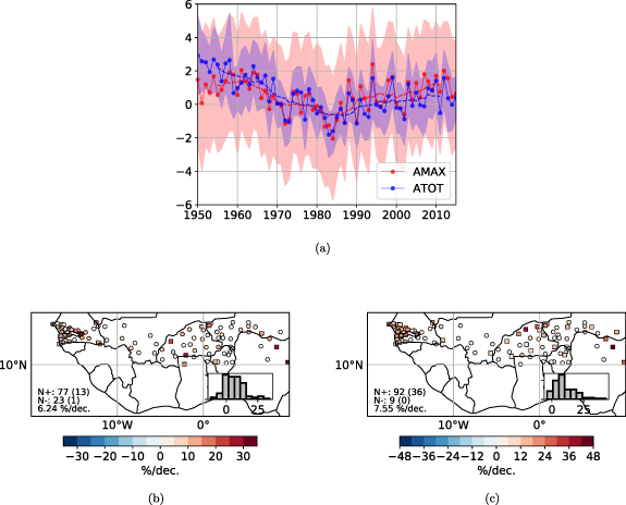
Figure 1. (a) Standardized Indices (SIs) of annual totals (ATOT, blue) and daily rainfall annual maxima (AMAX, red) for the 1950–2015 period. The color shading represent one standard deviation of spatial variability (see SM for the details). Dashed lines show 11 year running means. (b) AMAX and (c) ATOT Mann–Kendall relative trends (%/decade) over 1983–2015 at the 101 stations used in the study. Trends significant at the 5% level (p-value  0.05) are indicated with a square, non-significant ones with a circle. N+ and N− stand for the number of positive and negative trends, respectively (number of significant trends in parenthesis). The median trend across the stations is also indicated. The bottom right inboxes show the empirical probability distribution function of the trends. Note that one station has a null AMAX trend.
Download figure:
Standard image High-resolution imageTackling the three aforementioned issues involves dealing with the strong sampling effect inherent to Sahelian rainfall extremes: as shown in figure 1(a), the SI AMAX spatial variability (red shading) is twice as large as that of the SI ATOT (blue shading). Moreover, although the regional signal seems unequivocal, figure 1(b) shows that at the station scale, the significance of the positive AMAX trend is not so obvious, with only 13 stations out of 77 displaying a 5% level Mann–Kendall p-value (square markers); this is nearly 2.5 times less than for the ATOT (figure 1(c)). The study therefore makes use of a regional and non-stationary statistical model of extremes based on a generalized extreme value (GEV) distribution able to limit sampling effects (Panthou et al 2012, Chagnaud et al 2021). After being introduced in section 2 together with the dataset used, the model will allow to provide robust answers to the first two objectives (section 3) and to investigate the third one in a prospective way (section 4). Results are summarized and discussed in section 5.
2. Data and method
2.1. Raingauge data
The daily rainfall data are extracted from the BADOPLU data base (BAse de DOnnées PLUviomètres; see Le Barbé et al
2002, Lebel and Ali 2009, Panthou et al
2018) for the 1983–2015 period, following the years of lowest rainfall (figure 1(a)). The AMAX samples are extracted from stations having at least 26 valid years over the study period (i.e. ∼80%, see the quality control procedure in the SM of Panthou et al (2018) for the definition of a valid year). The regional AMAX sample gathers all stations meeting the time series completeness criteria located in a  box framing the 10∘ N–15∘ N, 20∘ W–10∘ E area and corresponding to the West African Sahel definition used in this study (figure S1(a)). Smaller regional samples are also built for investigating the sub-regional variability. The respective influences of the study area and of the study period starting year have been tested with no major influence on the results obtained (see section 3).
2.2. Regional non-stationary GEV (RNSGEV) model
In West Africa, daily rainfall at a given point is essentially associated with the passage of well delimited mesoscale convective system (MCS, e.g. Mathon et al 2002), meaning that daily rainfall amounts can be considered as independent or short-term dependent (Ali et al 2005, Gerbaux et al 2009). Moreover, working with AMAX values ensures the independence between block maxima. Under these conditions and according to the Extreme Value Theory (Coles 2001), annual maxima of daily rainfall amounts can be modeled with one type of GEV distributions (equation (S1)). As illustrated in figure 1(b), the behavior of AMAX series in a supposedly homogeneous region may vary significantly from station to station, due to their high sampling dispersion. Regional approaches based on a pooling of the point series allow for reducing the influence of this sampling dispersion, thus providing a more robust inference of the most uncertain components of the extreme value distribution, such as its tail behavior (e.g. Buishand 1991, Blanchet and Davison 2011). This is a central issue when it comes to estimating the probability—return period—of an extremely rare observed event or, reciprocally, the quantile—return level—for an extremely rare probability of occurrence (Papalexiou and Koutsoyiannis 2013). Moreover, regional pooling also improves the trend detection power of statistical methods (e.g. Fischer et al 2013, Fischer and Knutti 2014, Martel et al 2018). Here these two issues—robust statistical inference and trend detection ability—are tightly connected. Building on the work of Panthou et al (2012), we implement a regional GEV (RGEV) model wherein the location (µ) and scale (σ) parameters vary as a linear function of both the latitude and longitude (equation (S2)).
The RNSGEV model is obtained by expressing one or several GEV parameters as a function of time. Generalized linear models are used to model the time-varying GEV parameters (see Panthou et al 2013 and SM) since they are parsimonious as compared to non-linear models and because a linear form seems acceptable in a first approximation in view of the AMAX evolution displayed in figure 1(a). This means that any non-stationary parameter β of the RNSGEV distribution (β = µ, σ, ξ) may be expressed as:
Theoretically, there are thus 12 ( ) parameters to be estimated, a far too large number given the available information. Inferring the most appropriate model, based on a given sample, then pertains to identifying which additional parameter provides a significant improvement in terms of maximizing the model's likelihood function, starting from a reference time-stationary regional model M0. Practically, we rather minimize the model's negative log-likelihood (NLLH) function (see SM, section 1.4). The additional flexibility is then tested relying on the semi-parametric bootstrap procedure thoroughly described in Chagnaud et al (2021) (after Katz 2013, see SM, section 1.5). This procedure provides an empirical assessment of the significance of the various compared models while accounting for the spatial dependence between the pooled station samples. The uncertainty of the inferred parameters is quantified as the 5
 –95
–95 percentile range—corresponding to the 90% confidence interval (CI)—obtained from 200 bootstrapped sets of RNSGEV parameters.
3. Evidencing a regional trend
3.1. Non-stationarity of extreme rainfall captured by the GEV model
A preliminary visual analysis of our Sahelian dataset allows reducing the number of model formulations to be tested. First, the large sampling variance of ξ prevent any robust estimation of either ξ1, ξ2 or ξ3; ξ is thus assumed stationary in space and time (see also e.g. Renard et al 2006, Hanel et al 2009, Chagnaud et al 2021). The RNSGEV model cumulative distribution function (CDF) therefore reads:
Secondly, since neither the Mann–Kendall AMAX trend estimates (figure 1(b)) nor the point-wise non-stationary GEV models indicate any distinct spatial pattern of trends (figure S2), a spatially uniform relative trend over the study region is assumed. Therefore, a multiplicative expression for µ and σ is preferred to the additive one introduced in equation (1). It then remains to rule on the time non-stationarity parameters µ3 and σ3. Among the various tested models (SM, section 1.6), the one that proved the most parsimonious while providing the largest likelihood improvement according to the NLLH/bootstrap procedure is the M3 model (p-value  0.01, meaning that the improvement brought by this non-stationary model would happen by chance less than 1% of the time). The location and scale parameters of the M3 model are defined as follows:
where  . This model formulation is characterized by a similar time evolution of µ and σ (in relative terms). This evolution is estimated at 5%/decade ([2.7:7.5] 90% CI) over the considered period. Therefore, the statistical distribution is both shifted toward larger values and widened, as shown in figure 2. Note that the M1 (time-varying location parameter only) and M4 (independently time-varying location and scale parameters) models are also significant when compared to the time-stationary regional model (M0), but perform slightly worse than M3 (figure S3). Also worth mentioning is the fact that the trend undergoes only small variations when periods starting as far back as 1970 are considered (figure S4), demonstrating its significance even though, of course, its value is dependent on the year chosen to start the exploration (the linear formulation is not very flexible in this regard but again, provides the most parsimonious way to model this trend).

Figure 2. Probability density functions (PDFs) of the RNSGEV models M3 for the Niamey station with the total relative change (%) in 10-year (circle) and 50-year (triangle) return levels between 1983 (blue) and 2015 (green) indicated by the number above the arrows. The regional stationary model PDF and return levels are displayed in black. The color shadings correspond to the 90% CI obtained from 200 bootstrapped sets of parameters. The RNSGEV model parameter values are indicated in the upper right corner inset, corresponding, from left to right, to µ0, µ1, µ2, α3 and σ0, σ1, σ2 in equation (3).
Download figure:
Standard image High-resolution image3.2. Return levels
The T-year return level, defined as the daily rainfall amount having a probability  of being exceeded for a given year, is computed as follows at any point in space (
 ) and time (t):
where the location and scale parameters are computed according to equation (3) using the values shown in the inset box on figure 2. Comparing the value of a given return level at both ends (1983 and 2015) of the study period provides an estimate of the change in severity of an event of a given probability of occurrence (calculation details are provided in section 7 of the SM). This is illustrated in figure 2 for the 10-year (circle) and 50-year (triangle) return levels, with the 1983 distribution plotted in blue and the 2015 distribution in green. Also shown are the values of these two return levels under the stationarity assumption (black markers). It is noteworthy that the stationary CI (grey shading) is almost entirely distinct from the non-stationary 2015 CI (green shading), implying that computing return levels under the stationarity assumption likely leads to a significant (at the 90% level) under-estimation of the present-day value, and thus to the undersizing of infrastructures. Note that the formulation of the M3 model involves a similar relative change for all return levels and for all locations (a 16% increase, [8.8:24.7] 90% CI), a point that will be further discussed in section 3.4.
3.3. Return periods
Alternatively to changes in return levels, the non-stationarity can also be expressed as changes in return periods i.e. in the probability of occurrence of a given rainfall amount, as shown in figure 3: while 1983 return periods (horizontal axis) range from 2 to 1000 years, their 2015 counterparts (vertical axis) range from 1.4 to 360. Hence, the change in probability, defined as the  ratio, ranges from 1.4 ([1.2:1.5] 90% CI) for the 2-year return period to 2.8 ([1.8:4.6]) for the largest 1000-year return period.
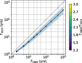
Figure 3. Return period change from 1983 to 2015 (90% CI in blue shading). The point color corresponds to the  ratio value (colorbar). The axis are in logarithmic coordinates for greater clarity.
Download figure:
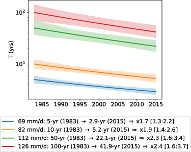
Standard image High-resolution imageThe potential to derive locally-relevant climate change metrics from the regional diagnostic is illustrated in figure 4 with the time evolution of various return periods corresponding to specific daily rainfall amounts at the Niamey station (13.5∘ N, 2.2∘ E). Take for instance a daily rainfall event of magnitude 82 mm d−1 (orange line): it is a 10-year rainfall in 1983 and it has become a 5.2-year rainfall in 2015; this rainfall amount is nearly twice as frequent at the end than it is at the start of the study period.
Figure 4. Time evolution of the 5- (blue), 10- (orange), 50- (green) and 100-year (red) return periods at the start of the study period (1983) at the Niamey station (13.5∘ N, 2.2∘ E). See the caption for the corresponding daily rainfall amount and return period values. The numbers in brackets correspond to the 90% CI of the  ratios 3(return period 90% CI are shown with the color shading).
Download figure:
Standard image High-resolution image
The ability of looking at the effects of non-stationarity either in terms of return levels or in terms of return periods is a clear benefit of the statistical modeling framework and an important step forward from previous observationally-based studies (Panthou et al 2014, Taylor et al 2017). The metric to be used, either a change in magnitude for an event with a given probability or a change in probability of a fixed magnitude event will depend on the application and the related risk management policy.
3.4. Simplicity versus complexity
The regional approach presented above allows for a robust detection of the non-stationarity of the annual rainfall maxima in the Sahel, with both a significant shift toward larger values and an increase of their interannual variability, a conclusion that could not be drawn from analyzing separately the available point series. The significance of this non-stationarity is quantified through the NLLH/bootstrap procedure and its effect is straightforwardly derived in terms of increasing return levels and decreasing return periods.
These achievements leave room for debating whether alternate models would more faithfully depict the rainfall regime evolution in this region. The discussion comes down to asking whether we could use a more complex model—and for which benefits—having in mind that, among the four models presented in the SM, three (M1, M2, M3) have the same number (8) of parameters and one (M4) has 9. Two of the 8-parameter models (M1 and M3) were found to be significantly better than the stationary model, M3 being the most significant. M4 is also significant, but less than M3.
M4 is less significant but its additional free parameter gives it a greater flexibility, allowing for an independent time-evolution of µ (4.9%/decade) and σ (3.1%/decade). In M3, µ and σ are assumed to present the same relative evolution, with the effect that return levels corresponding to any probability of occurrence undergo the same relative change. As further investigated in section 4, a different evolution of µ and σ might correspond to a more realistic account of the underlying changes of the rainfall regime. Choosing between the most significant model and a less significant but possibly more realistic alternative is not a matter easily solved, especially since the M4 model provides return level estimates close to those given by M3, yet with a slightly smaller rate of increase (∼4%/decade). That is a fairly open question, keeping in mind that it is well possible that with longer time series M4 could prove as significant as M3. This, however, is just a conjecture at that point.
A still more complex model would be to assume that the shape parameter of the RGEV distribution, ξ, could also vary in time. Given the high sampling variance of ξ, detecting a trend of its value is out of reach with the dataset used here and we thus kept to the conservative hypothesis that it is constant. Exploring whether the increase of return levels could be magnified for large return periods—typically beyond T = 100 years—remains a challenge, and their evolution as provided by the M3 model should be considered very cautiously.
Another issue relates to the spatial behavior of the trend, assumed here to be uniform in relative terms. This is probably not strictly true, as various mechanisms may modulate the overall regional trend. For instance, two types of atmospheric disturbances called African Easterly Waves (AEWs) support the development and propagation of sahelian storms: those originating to the north of the African Easterly Jet and those to the south, accounting for 71% and 29%, respectively, of the total number of AEWs (Chen 2006). Since these two types of AEWs have different genesis mechanisms, one may expect a distinct response to any large-scale forcing, thus potentially influencing the interannual variability as well as a long-term trend in different ways. Here, however, there is no detectable latitudinal gradient affecting the evolution of the regime of extreme rainfall (see SM, section 8.2). Likewise, the trends computed on smaller areas display a striking zonal similarity (SM, section 8.1). As a consequence of this spatial homogeneity, the signal is more robustly detected when considering the Sahel as a whole. Moreover, the derived metrics are associated with narrower CI as compared to their sub-regional counterparts (figure S7 and table 1 in the SM), evidencing a more robust ability for detecting trends when working on large regions, provided that they are climatologically homogeneous (e.g. Donat et al 2016). Whether the absence of spatial gradient is due to a limited detection ability or to the dominance of a mechanism acting on the whole region remains elusive at this point. Again, it may happen that with longer time series, a finer description of the spatial pattern of the trend could emerge.
All in all, the regional vision provided here may be considered as a first order representation of an undoubtedly more complex reality. It is only by developing and maintaining regional- and local-scale in-situ rainfall monitoring systems that we will obtain the necessary information for a more detailed characterization of this reality, needed to support locally-relevant decision-making in various fields pertaining to agriculture, flood warning or water resources management.
4. More severe extreme rainfall as a consequence of an overall rainfall regime evolution
An increasing frequency of heavy rainfall may result from two essential climatological trends: a change in rainfall intensity distribution (mean, variance or higher moments) and/or an increase of the number of rainy events per year. The latter produces a global shift of the AMAX distribution, meaning a similar relative decrease of the return periods for the whole spectrum of intensities, while the former produces a larger decrease of the return periods for larger intensities, as illustrated in figure 4. From their empirical analysis of the evolution of Sahelian daily rainfall from 1950 to 2014, Panthou et al (2018) revealed that both the average daily rainfall (R) and the number of rainy events (N) have been increasing over the past three decades. However, they point to R starting to increase a bit earlier and at a much higher rate than N. Concurrent with this, figure 1(a) shows that at the Sahelian scale the regime of extreme rainfall (red line) might be changing more rapidly than that of annual totals (blue line). In order to investigate to which extent the GEV statistical framework allows to capture this important climatological trend, we will resort to a degenerated version of the M4 model where ξ is prescribed to 0 while µ and σ are free to vary independently in time (hereafter M4 ). M4
). M4 and M3 have consequently the same number of degrees of freedom but M4
 is slightly less optimal than M3 in describing the time evolution on our data. However, it is still able to detect the intensification trend (not shown). A GEV model with ξ = 0 is commonly known as the Gumbel law. It results from a point process whose values are asymptotically exponentially distributed. Assuming rainfall occurrences to follow a Poisson process with an exponential distribution of the durations between two successive events, the following relationship between the parameters of the point rainfall process and the parameters of the extreme rainfall distribution can be derived:


where λ is the mean number of rainfall events per year and α is the mean daily rainfall intensity, while µ and σ are the two parameters of the Gumbel distribution. In M4 , the parameters of the Gumbel distribution are a function of space and time, and its CDF reads:
The parameters are inferred with the NLLH/bootstrap procedure used in section 3. The relative augmentation of the parameters of equations (5) and (6) between 1983 and 2015 are:

This leads to estimate an increase of daily rainfall intensity of 10.7% over 33 years, a value fully consistent with the ∼11% found by Panthou et al (2018) in their analysis of the raw daily rainfall data over the period 1980–2014. This M4 model gives similar results to M3 as far as the impact on return period is considered: they have been divided by a factor close to or larger than 2 for intensities ranging from 80 mm d−1 (47% decrease) to 120 mm d−1 (60% decrease) (see table 3 in the SM), thus confirming the robustness of the non-stationary signal in that range of occurrences. The advantage of resorting to M4
 for exploring the climatological context is that it allows deciphering the respective shares of the return period diminution associated with the increase of the mean intensity of the rain events, on the one hand, and with the increase of the number of events per year, on the other hand. This is done by computing which diminution would have been caused by
  being equal to
  (in that case λ is unchanged). It turns out that the sole modification of σ accounts for 80% to 90% of the diminution of the return periods (83% for 80 mm d−1 to 89% for 120 mm d−1, see calculation details in section 9 of the SM), confirming the large predominance of more intense rainfall events for explaining the change of the statistical distribution of extreme rainfall in the region.
5. Main results and concluding remarks
Using a regional non-stationary GEV model on an extensive raingauge dataset covering the West African Sahel, we detect a 5%/decade ([2.7:7.5] 90% CI) increase in the location and scale parameters of the daily rainfall extremes distribution over the 1983–2015 period. This trend leads to an overall 16% increase of return levels and to a 50%–60% decrease of return periods, with larger decreases for the strongest events. It is highly significant (p-value  1%) and robust over the last 30–40 years, although its magnitude may vary slightly. Hence, we stress that the figures reported here should be considered by engineers and decision-makers for planning adaptation strategies as far as water resources and water-related risks are concerned, though how to use this information to project strategies remains an open question (see e.g. Sharma et al
2021). Moreover, because these figures are not to remain constant in a rapidly changing climate, it is essential to regularly update them; it is thus crucial to continuously monitor the evolution of the daily rainfall regime at the regional scale.
1%) and robust over the last 30–40 years, although its magnitude may vary slightly. Hence, we stress that the figures reported here should be considered by engineers and decision-makers for planning adaptation strategies as far as water resources and water-related risks are concerned, though how to use this information to project strategies remains an open question (see e.g. Sharma et al
2021). Moreover, because these figures are not to remain constant in a rapidly changing climate, it is essential to regularly update them; it is thus crucial to continuously monitor the evolution of the daily rainfall regime at the regional scale.
One may question whether this trend in extreme rainfall is not just a consequence of the rebound of the annual rainfall, itself attributed to a combination of sea surface temperature (SST) variability (Mohino et al
2011, Marvel et al
2020), anthropogenic aerosols emissions shrinking (Marvel et al
2020) and increasing greenhouse gases (GHG) concentration (Dong and Sutton 2015). Two key elements shed some light on this debate. First, extremes have been providing an increasing share of the annual rainfall (as already reported in Panthou et al
2018). Secondly, while the historical drought was characterized by a drastic decrease of the number of rain events (Le Barbé et al
2002), the annual rainfall rebound at the end of the 20 century is mostly associated with an increase of rain event intensity (Giannini et al
2013, Panthou et al
2018). We show here that this increase in mean daily rainfall intensity since the early 80s accounts for about 80% of the increase in extreme daily rainfall amounts, the remaining 15%–20% being due to an increasing number of wet days. Thus, it is not just a return to the antecedent rainfall regime but the entry in an intensified hydro-climatic era, in the sense defined by Giorgi et al (2011).
century is mostly associated with an increase of rain event intensity (Giannini et al
2013, Panthou et al
2018). We show here that this increase in mean daily rainfall intensity since the early 80s accounts for about 80% of the increase in extreme daily rainfall amounts, the remaining 15%–20% being due to an increasing number of wet days. Thus, it is not just a return to the antecedent rainfall regime but the entry in an intensified hydro-climatic era, in the sense defined by Giorgi et al (2011).
The detected trend of 5%/decade being stronger than the one expected from the sole Clausius-Clapeyron effect is also food for thought. The unique combination of changes in large scale forcing factors (SST, aerosols, GHG) mentioned above might have induced a reinforcement of the AEWs, which have long been known to play a key role in initiating and driving intense Sahelian MCS (e.g. Peters and Tetzlaff 1988, Fink and Reiner 2003). Recent studies have indeed highlighted that AEWs are involved in some of the heaviest storms ever recorded in the Sahel (Engel et al 2017, Lafore et al 2017, Vizy and Cook 2021). Our capacity to anticipate how the rainfall intensification will evolve over the next decades thus largely depends on an improved understanding of the interactions between large scale forcings and an array of thermodynamical and dynamical processes (Tomassini 2018).
Data availability statement
The data generated and/or analysed during the current study are not publicly available for legal/ethical reasons but are available from the corresponding author on reasonable request.
Acknowledgments
The authors especially wish to express gratitude for the enlightening discussions they had with the late Françoise Guichard on the results presented here. They are also grateful to Y Sane and O Ndiaye from the ANACIM for the provision of the data over Senegal and to two anonymous reviewers for their insightful comments.
Conflict of interest
The authors declare no competing interests.