

Abstract
Cryospheric long-term timeseries get increasingly important. To document climate-related effects on long-term viscous creep of ice-rich mountain permafrost, we investigated timeseries (1995–2022) of geodetically-derived Rock Glacier Velocity (RGV), i.e. spatially averaged interannual velocity timeseries related to a rock glacier (RG) unit or part of it. We considered 50 RGV from 43 RGs spatially covering the entire European Alps. Eight of these RGs are destabilized. Results show that RGV are distinctly variable ranging from 0.04 to 6.23 m a−1. Acceleration and deceleration at many RGs are highly correlated with similar behaviour over 2.5 decades for 15 timeseries. In addition to a general long-term, warming-induced trend of increasing velocities, three main phases of distinct acceleration (2000–2004, 2008–2015, 2018–2020), interrupted by deceleration or steady state conditions, were identified. The evolution is attributed to climate forcing and underlines the significance of RGV as a product of the Essential Climate Variable (ECV) permafrost. We show that RGV data are valuable as climate indicators, but such data should always be assessed critically considering changing local factors (geomorphic, thermal, hydrologic) and monitoring approaches. To extract a climate signal, larger RGV ensembles should be analysed. Criteria for selecting new RGV-sites are proposed.
Export citation and abstract BibTeX RIS

Original content from this work may be used under the terms of the Creative Commons Attribution 4.0 license. Any further distribution of this work must maintain attribution to the author(s) and the title of the work, journal citation and DOI.
1. Introduction
Rock glaciers (RGs) are striking landforms of ice-(super)saturated permafrost in periglacial mountain environments [1–4]. According to the Rock Glacier Inventories and Kinematics (RGIK) initiative of the International Permafrost Association (IPA) [5], RGs are defined as debris landforms generated by the former or ongoing creep of perennially frozen ground rich in ice. They are detectable in the landscape with a distinctive front and lateral margins as well as occasionally ridge-and-furrow surface topography. Permafrost creep refers to the combination of both internal deformation within the ice of the frozen material (creep of permafrost body sensu stricto) and shearing at one or more distinct horizons within or near the base of the frozen body [4–6]. The latter is not strictly related to the occurrence of RGs but can also be the motion mechanism of further mass movements in permafrost conditions. RGs are therefore key landforms for understanding the effects of past, present, and projected climate change and thus environmental conditions in the periglacial process domain [7, 8].
RGs are widespread in the European Alps (5769 RGs in Austria, [9]; 3261 RGs in France, [10]) and globally [11]. Intact RGs consist of poorly sorted, mostly angular rock material, ice from deep and long-term freezing (mostly interstitial, segregation or massive ice) with in cases remains of buried surface ice (mostly from perennial ice patches or small retreating glaciers; [12]), water, and air. RGs develop over centuries to millennia as shown by relative or numerical dating approaches [13–16]. Even though some RGs contain remains of buried surface ice, local climate conditions keeping the subsurface frozen for hundreds to thousands of years are indispensable for their formation and preservation [17]. Environmental conditions are not stationary at such time scales. Thus, RGs may experience strong variations in their rate of nourishment in debris and their overall ice content over time [18]. Such variations might lead to multi-unit RG systems with several simple or complex superimposed units ([19]; figure 1). The frozen materials of active RGs typically creep downslope with horizontal surface velocities of centimetres to metres per year [20, 21]. In case of the destabilization of RGs, velocities substantially and heterogeneously increase impacting the surface morphology forming cracks, scarps, or crevasses, which might gradually lead to RG disintegration [22–27].
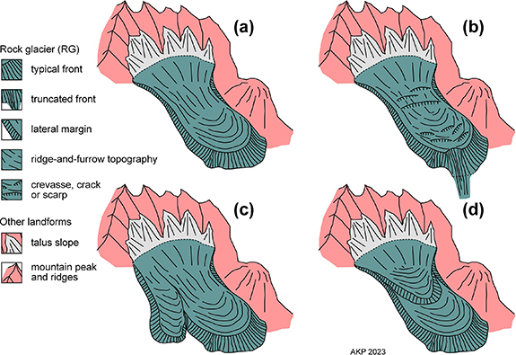
Figure 1. Different examples of talus-connected RG systems delineated by the extended geomorphological footprint: (a) mono-unit rock glacier system—simple unit; (b) mono-unit rock glacier system—complex unit with disintegration signs (crevasses, cracks or scarps) and a partly-truncated front; (c) multi-unit rock glacier system—e.g. two adjacent units; (d) multi-unit rock glacier system—e.g. two overlapping units (for explanation of the terms used in this graphic see [5, 19]).
Download figure:
Standard image High-resolution imageWhereas debris and ice input to the RG system is vital for its millennial development, the measured decadal kinematics (i.e. horizontal and vertical surface elevation change over time) has been discussed jointly with other environmental parameters such as ground temperature or hydrology to understand the RG-climate-relationship [4, 28, 29]. The key relationship is that the interannual variability of rock glacier velocity in general as a generic term follows permafrost temperature and all related consequences, especially temperature-dependent viscosity and unfrozen water content. In addition, availability and advection of surface water into the RG sediments affects the creep behaviour by changing the pore-water pressure [30]. The combined geomorphological, soil thermal, hydrological, and climatic forcing of rock glacier creep highlights the environmental relevance of monitoring such landforms. Therefore, 'Rock Glacier Velocity' or ('RGV' became an associated product of the Essential Climate Variable (ECV) permafrost [31] within the Global Climate Observing System in October 2022 [32, 33]. RGV, contrasting to the generic usage of rock glacier velocity as described above, is defined as a spatially averaged interannual horizontal velocity timeseries related to a RG unit or a part of it. Thus, RGV is a climate indicator that reflects impacts from climate change on cold mountain environments without reducing climate change to only temperature. Summary reports on RGV, presenting this topic in a broader environmental framework, have recently been published, covering such data from different parts of the world [7]. This implies that operational monitoring of RGs, as part of permafrost observation, is increasingly important [21, 34].
In this contribution we discuss 50 RGV measured at 43 RGs in the European Alps. We focus on the time period 1995–2022 due to increased RGV monitoring activities since the mid-1990s and discuss relations to climatic and environmental factors. This joint research effort is a continuation of earlier activities [35–37] but presents a more comprehensive database for the entire European Alps. The aims of this study are: (a) compilation of a homogenized dataset of RGV based on geodetic methods for the time period 1995–2022 for the European Alps, (b) presentation of long-term monitoring results of the collected timeseries, and (c) assessment of the influence of different environmental variables driving the temporal and spatial patterns of RGV evolution in the European Alps.
2. Studied rock glaciers
The European Alps (hereafter Alps) are the most prominent mountain range entirely located in Europe and reach a maximum elevation of 4808 m asl at Mont Blanc/Monte Bianco. The mountain range separates the marine west-coast climates of Western Europe from the Mediterranean areas to the south related to the arch shape of the mountain range. The Alps act as a barrier in relation to the mid-latitude cyclones that cross Central Europe usually from west to east. Climatic features include distinct gradients in all three spatial dimensions of space (latitude, longitude, elevation) leading to four main types of transitions: south-north (from Mediterranean to temperate climate), west-east (from humid-oceanic to dry-continental), peripheral-central (humid-cool margin of the Alps to dry-warm inner alpine climate), and hypsometric (altitudinal zonation) [38, 39]. Around 6220 km2 of the Alps are underlain by permafrost if a permafrost index of ⩾0.5 is used as a realistic threshold for permafrost existence [40].
In this study, we selected 43 RGs (table 1) with appropriate data located between latitude 45°01'00''N and 46°59ʹ38''N and between longitude 6°23ʹ57''E and 13°17ʹ06''E. The RG sites cover a west-east distance of 570 km and a north-south one of 220 km (figure 2). Our dataset includes 1 RG in France, 31 in Switzerland, 5 in Italy and 6 in Austria. Almost all the studied landforms are considered as RGs as previously defined. The only possible exception is a glacial-permafrost composite landform I05/Amola [41]. Some RGs are also close to present glaciers. The creep of such RGs may have been influenced by changes in glaciation (e.g. C23/Gruben; [42, 43]).

Figure 2. Study sites: (a) location of the 43 investigated RGs in the Alps grouped into seven different regions. Inset map (b) refers to south-western Switzerland and north-western Italy with permafrost distribution visualising that the studied RGs are dominantly in marginal mountain permafrost positions. The four automatic weather stations considered in the text are localized (Besse 1520 m asl, Säntis 2502 m asl, Zugspitze 2960 m asl, Sonnblick 3109 m asl). For explanation of RG-codes see table 1. Data sources: [44] (topography), [45] (perimeter of Alps), [46] (glaciers in 2015), [40] (permafrost).
Download figure:
Standard image High-resolution imageTable 1. Summary of the 43 studied rock glaciers with one key publication per site for more information. Relevant for the codes: A = Austria, F = France, I = Italy, C = Switzerland; Regions: AA = Austrian Alps; FA = French Alps, IA = Italian Alps, LV = Lower Valais, UV = Upper Valais, EN = Engadine, TI = Ticino.
| Cod. | Rock glacier/Region | Lat N (°) | Long E (°) | Elev. range (m asl) | Area (km2) | Asp. (class) | Lith. | Key publication |
|---|---|---|---|---|---|---|---|---|
| A03 | Weissenkar/AA | 46°57'29'' | 12°45'11'' | 2610–2720 | 0.125 | W | ms | Kellerer-Pirklbauer and Kaufmann [28] |
| A04 | Hinteres Langtalkar/AA | 46°59'11'' | 12°46'48'' | 2455–2700 | 0.168 | NW | ms | Kellerer-Pirklbauer and Kaufmann [47] |
| A05 | Dösen/AA | 46°59'11'' | 13°17'06'' | 2340–2650 | 0.194 | W | og | Kellerer-Pirklbauer et al [48] |
| A06 | Äußeres Hochebenkar/AA | 46°50'01'' | 11°00'36'' | 2420–2870 | 0.423 | NW | ms,pg | Hartl et al [49] |
| A08 | Tschadinhorn/AA | 46°59ʹ38'' | 12°41ʹ47'' | 2575–2800 | 0.061 | NW | am | Kaufmann et al [50] |
| A09 | Leibnitzkopf/AA | 46°55ʹ51'' | 12°42ʹ43'' | 2450–2580 | 0.062 | W | ms | Kaufmann et al [51] |
| F01 | Laurichard/FA | 45°01ʹ00'' | 6°23ʹ57'' | 2420–2640 | 0.084 | N | gr | Thibert and Bodin [52] |
| I01 | Lazaun/IA | 46°44ʹ43'' | 10°45ʹ13'' | 2495–2810 | 0.175 | NNE | ms,pg | Fey and Krainer [53] |
| I02 | Gran Sometta/IA | 45°55ʹ13'' | 7°40ʹ13'' | 2640–2770 | M: 0.240 S: 0.077 | NNW | cs | Bearzot et al [54] |
| I03 | Napfen/IA | 46°58ʹ06'' | 12°07ʹ42'' | 2565–2842 | 0.410 | NW | ms,pg | Damm [55] |
| I04 | Maroccaro/IA | 46°13ʹ02'' | 10°34ʹ28'' | 2750–2870 | 0.025 | SW | to | Seppi et al [41] |
| I05 | Amola/IA | 46°12ʹ04'' | 10°42ʹ43'' | 2310–2580 | 0.124 | NNE | to | Seppi et al [41] |
| C01 | Aget-Rogneux/LV | 46°00ʹ35'' | 7°14ʹ24'' | 2810–2890 | 0.038 | SE | mm | Wee and Delaloye [56] |
| C02 | Mont-Gelé B/LV | 46°05ʹ49'' | 7°17ʹ22'' | 2600–2740 | 0.022 | NE | gn | Delaloye et al [21] |
| C03 | Mont-Gelé C/LV | 46°05ʹ49'' | 7°17ʹ13'' | 2620–2820 | 0.035 | N | gn | Delaloye et al [21] |
| C04 | Tsarmine/LV | 46°02ʹ47'' | 7°30ʹ31'' | 2480–2650 | 0.052 | W | og | Vivero et al [27] |
| C05 | Becs-de-Bosson/LV | 46°10ʹ23'' | 7°30ʹ41'' | 2610–2850 | 0.175 | NW | cs | Delaloye et al [21] |
| C06 | Gemmi-Furggentälti/UV | 46°24'23'' | 7°37'53'' | 2440–2700 | 0.027 | NNW | ls | Delaloye et al [21] |
| C07 | Hungerlitälli 1/UV | 46°11'14'' | 7°43'28'' | 2630–2780 | 0.049 | NNW | og,ph | Delaloye et al [21] |
| C08 | Hungerlitälli 3/UV | 46°11'11'' | 7°43'00'' | 2515–2650 | 0.048 | NW | og,ph | Delaloye et al [21] |
| C09 | Büz North/EN | 46°32'00'' | 9°49'03'' | 2775–2840 | 0.017 | NNE | sh | Ikeda et al [57] |
| C10 | Petit-Vélan/LV | 45°54'51'' | 7°13'51'' | 2520–2810 | 0.078 | NE | gn | Delaloye and Morard [58] |
| C11 | Lac des Vaux B/LV | 46°05'58'' | 7°16'33'' | 2720–2800 | 0.007 | NW | gn | Delaloye et al [21] |
| C12 | Lués Rares/LV | 46°06'13'' | 7°17'45'' | 2320–2450 | 0.029 | NE | gn | Delaloye et al [21] |
| C13 | Les Cliosses/LV | 46°08'40'' | 7°30'10'' | 2450–2550 | 0.038 | W | cs | Delaloye et al [21] |
| C14 | Tsaté-Moiry 1/LV | 46°06'40'' | 7°33'15'' | 2680–2850 | 0.033 | NE | cs | Lambiel [59] |
| C15 | Tsaté-Moiry 2/LV | 46°06'35'' | 7°33'20'' | 2720–2850 | 0.056 | NE | cs | Lambiel [59] |
| C17 | Grosse Grabe/UV | 46°09'03'' | 7°49'13'' | 2600–2740 | 0.064 | WNW | ag | Delaloye et al [23] |
| C18 | Gugla-Bielzug/UV | 46°08'20'' | 7°49'06'' | 2600–2820 | 0.095 | W | ms | Delaloye et al [23] |
| C19 | Dirru/UV | 46°07'18'' | 7°49'04'' | 2530–2940 | 0.077 | WNW | gn | Delaloye et al [23] |
| C21 | Grosses Gufer/UV | 46°25'31'' | 8°04'57'' | 2380–2600 | 0.176 | NW | gn | Delaloye et al [21] |
| C23 | Gruben/UV | 46°10'26'' | 7°57'57'' | 2770–2890 | 0.364 | WSW | gn | Gärtner-Roer et al [42] |
| C24 | Monte Prosa A/TI | 46°33'52'' | 8°34'46'' | 2440–2570 | 0.046 | N | gr | Mari [60] |
| C25 | Monte Prosa B/TI | 46°33'46'' | 8°34'28'' | 2450–2530 | 0.025 | NW | gr | Mari [60] |
| C26 | Stabbio di Largario/TI | 46°28'40'' | 8°59'10'' | 2230–2550 | 0.116 | N | og | Scapozza et al [61] |
| C27 | Piancabella/TI | 46°27'02'' | 9°00'10'' | 2450–2550 | 0.023 | NE | gn | Scapozza et al [62] |
| C29 | Ganoni di Schenadüi/TI | 46°33'20'' | 8°44'50'' | 2480–2640 | 0.067 | N | og | Delaloye et al [21] |
| C30 | Muragl/EN | 46°30'24'' | 9°55'42'' | 2490–2750 | 0.151 | NW | gd,gr | Cicoira et al [30] |
| C31 | Murtèl-Corvatsch/EN | 46°25'44'' | 9°49'19'' | 2630–2800 | 0.070 | WNW | gd,gr | Cicoira et al [30] |
| C32 | Marmugnun/EN | 46°25'41'' | 9°49'09'' | 2650–2700 | 0.044 | NW | gd,gr | Delaloye et al [21] |
| C33 | Chastelets/EN | 46°25'44'' | 9°48'48'' | 2650–2700 | 0.034 | NW | gd,gr | Delaloye et al [21] |
| C34 | Tsavolire/LV | 46°09'57'' | 7°30'30'' | 2800–2900 | 0.034 | NW | cs | Delaloye and Staub [63] |
| C35 | Lapires/LV | 46°06'00'' | 7°17'00'' | 2360–2650 | 0.005 | NNE | ps | Mollaret et al [64] |
a area derived from GIS-based delineation by the different authors. b dominant lithology: ms = mica schist, og = ortho gneiss, pg = para gneiss, gn = gneiss, am = amphibolite, gr = granite, cs = calcareous schist, to = tonalite, mm = various metamorphic rocks (e.g. quartzites), ls = limestone, ph = phyllite, sh = shale, ag = augen gneiss, gd = granodiorite, ps = prasinite. c part of the Swiss Permafrost Monitoring Network (PERMOS), n = 17 [65]. d M = main, S = secondary. e distinct signs of destabilisation in 1995–2022 with larger cracks and crevasses (reaction type 2 or 3 according to Schoeneich et al [24]. f glacier forefield; back-creeping push moraine. g talus slope with a small rock glacier. h glacial-permafrost composite landform. i further name 'Yettes Conjà'. j further name 'Réchy'.
The investigated RGs terminate at elevations from 2230 to 2810 m asl, extend over elevation ranges from 50 to 450 m, cover an area of 0.005 (C35/Lapires) to 0.42 km2 (A06/Äußeres-Hochebenkar), and are mostly north-oriented (figure 3; table 1). Metamorphic rocks build-up 34 RGs (mostly gneiss and schist), 7 RGs are composed of igneous rocks (granodiorite, granite), and two of sedimentary rocks (limestone, shale). Eight RGs showed distinct signs of destabilization in the observation period with cracks, crevasses, or scarps (tables 1 and 2; reaction type 2 [accelerated displacement rate of part or whole of a RG] or 3 [dislocation and rupture of the lower part of a RG] according to [24]).
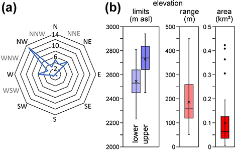
Figure 3. Distribution and some morphometric characteristics of the 43 RGs studied: (a) dominant aspect and (b) upper and lower elevation limit, elevation range, and surface area.
Download figure:
Standard image High-resolution imageTable 2. Summary of monitoring history and study design for each of the 43 investigated RGs with reference to the responsible institutions. Data since 1995 are considered in this study. Data gaps are not listed in this table.
| Cod. | Rock glacier/Re | Monit initiation | Monit units | Geodetic metho (present) | No. pts all (n) | No. pts reference (n) | Years with RGV data (n) | Res. inst. |
|---|---|---|---|---|---|---|---|---|
| A03 | Weissenkar/AA | 1997 | 1 | GNSS | 18 | 18 | 19 | 12,1 |
| A04 | Hinteres Langtalkar/AA | 1999 | 2 (U/L) | GNSS | 38 | U9; L6 | U23/L23 | 12,1 |
| A05 | Dösen/AA | 1995 | 1 | GNSS | 34 | 11 | 25 | 12,1 |
| A06 | Äußeres Hochebenkar/AA | 1951 (1938 | 1 | GNSS | 46 | 39 | 23 | 10 |
| A08 | Tschadinhorn/AA | 2014 | 1 | GNSS | 14 | 14 | 8 | 12,1 |
| A09 | Leibnitzkopf/AA | 2010 | 1 | GNSS | 15 | 15 | 12 | 12,1 |
| F01 | Laurichard/FA | 1979 | GNSS | 35 | 5 | 27 | 2,6,18 | |
| I01 | Lazaun/IA | 2006 | GNSS | 52 | 39 | 5 | 13 | |
| I02 | Gran Sometta/IA | 2012 (M) 2015 (S) | 2 (M/S) | GNSS | 62 | M16; S8 | M10/S7 | 3,14 |
| I03 | Napfen/IA | 1992/93 | 1 | Laser dist. | 95 | 5 | 21 | 9,13 |
| I04 | Maroccaro/IA | 2001 | 1 | Total st. | 25 | 23 | 14 | 7,16,19 |
| I05 | Amola/IA | 2001 | 1 | Total st. | 25 | 24 | 15 | 7,16,19 |
| C01 | Aget-Rogneux*/LV | 2001 | GNSS | 79 | 9 | 21 | 3 | |
| C02 | Mont-Gelé B/LV | 2000 | 1 | GNSS | 37 | 23 | 22 | 4 |
| C03 | Mont-Gelé C/LV | 2000 | 1 | GNSS | 34 | 19 | 20 | 4 |
| C04 | Tsarmine/LV | 2004 | 2 (U/L) | GNSS | 53 | U4; L3 | U18/L18 | 3,4 |
| C05 | Becs-de-Bosson/LV | 2004 | 2 (G1/LG2/U) | GNSS | 206 | G1/L 45; G2/U 21 | U18/L18 | 3 |
| C06 | Gemmi-Furggentälti/UV | 1998 | 1 | GNSS | 70 | 5 | 24 | 3 |
| C07 | Hungerlitälli 1/UV | 2001 | 1 | Total st. | 24 | 24 | 17 | 5 |
| C08 | Hungerlitälli 3/UV | 2002 | 1 | Total st. | 27 | 14 | 18 | 5 |
| C09 | Büz North/EN | 1998 | 1 | GNSS | 13 | 4 | 21 | 11,15 |
| C10 | Petit-Vélan/LV | 2005 | 1 | GNSS | 52 | 5 | 17 | 3 |
| C11 | Lac des Vaux B/LV | 2005 | 1 | GNSS | 31 | 8 | 15 | 4 |
| C12 | Lués Rares/LV | 2006 | 1 | GNSS | 21 | 10 | 16 | 4 |
| C13 | Les Cliosses/LV | 2006 | 1 | GNSS | 33 | 24 | 16 | 4 |
| C14 | Tsaté-Moiry 1/LV | 2005 | 1 | GNSS | 53 | 6 | 15 | 4 |
| C15 | Tsaté-Moiry 2/LV | 2005 | 1 | GNSS | 25 | 16 | 13 | 4 |
| C17 | Grosse Grabe/UV | 2007 | 1 | GNSS | 12 | 3 | 14 | 3 |
| C18 | Gugla-Bielzug/UV | 2007 | 1 | GNSS | 44 | 5 | 15 | 3 |
| C19 | Dirru/UV | 2007 | 2 (U/L) | GNSS | 75 | U10; L24 | U15/L15 | 3 |
| C21 | Grosses Gufer/UV | 2007 | 1 | GNSS | 65 | 16 | 15 | 3 |
| C23 | Gruben/UV | 2012 | 1 | GNSS | 43 | 10 | 10 | 3 |
| C24 | Monte Prosa A/TI | 2009 | 1 | GNSS | 34 | 16 | 10 | 3 |
| C25 | Monte Prosa B/TI | 2009 | 1 | GNSS | 24 | 2 | 13 | 3 |
| C26 | Stabbio di Largario/TI | 2009 | 2 (M/S) | GNSS | 33 | M21; S4 | M12/S11 | 17 |
| C27 | Piancabella/TI | 2009 | 1 | GNSS | 28 | 20 | 14 | 17 |
| C29 | Ganoni di Schenadüi/TI | 2009 | 2 (U/L) | GNSS | 35 | U3; L15 | U11/L11 | 17 |
| C30 | Muragl/EN | 2009 | 1 | Total st. | 20 | 20 | 13 | 5 |
| C31 | Murtèl-Corvatsch/EN | 2009 | 1 | Total st. | 11 | 11 | 13 | 5 |
| C32 | Marmugnun/EN | 2009 | 1 | Total st. | 9 | 9 | 11 | 5 |
| C33 | Chastelets/EN | 2009 | 1 | Total st. | 5 | 5 | 11 | 5 |
| C34 | Tsavolire/LV | 2012 | 1 | GNSSp | 1 | 1 | 9 | 3 |
| C35 | Lapires/LV | 2013 | 1 | GNSS | 11 | 4 | 15 | 3 |
a initiation of RGV monitoring—data gaps are not indicated. b number of monitored units—in case of two units: U = upper part; L = lower part, M = main unit, S = secondary unit, G1/L = group 1, mostly lower part, G2/U = group 2, mostly upper part. c geodetic method: GNSS = annual GNSS campaign, laser dist. = laser distance measurement device, total st. = total station, GNSSp = permanent GNSS instrument. d number of measurement points. e number of points to calculate the average value—reference points. f institution according to the affiliation list. g considered in PERMOS. h terrestrial photogrammetry monitoring initiation. i distinct signs of destabilisation in 1995–2022 with larger cracks and crevasses.
Figure 4 depicts examples of the 43 RGs. F01/Laurichard (figure 4(a)) is a well-developed, talus-connected mono-unit RG system (cf figure 1(a)). C30/Muragl (figure 4(b)) is a multi-unit RG system with partly overlapping units and several lobes (cf figures 1(c) and (d)). The two other examples show other less common morphological characteristics. A04/Hinteres-Langtalkar (figure 4(c)) is a multi-unit RG with two rooting zones (both formerly occupied by a glacier) with distinct disintegration features and an advancing, partly collapsing front (figure 1(b)). Finally, C04/Tsarmine (figure 4(d)) is a mono-unit RG system with a well-developed truncated front, which supplies a steep alpine torrent with debris (figure 1(b)).
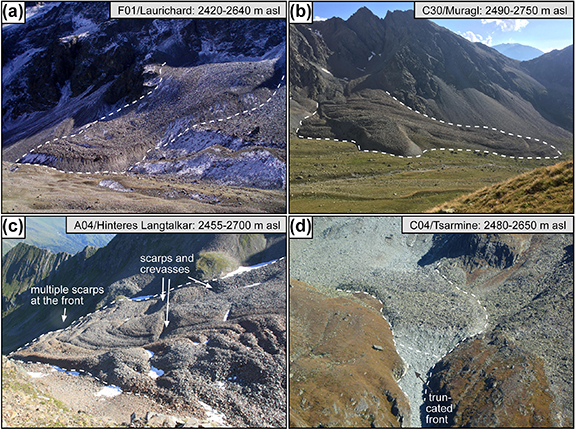
Figure 4. Four examples of investigated RGs: (a) Laurichard RG—mono-unit rock glacier system; (b) Muragl RG—multi-unit rock glacier system; (c) Hinteres Langtalkar RG—multi-unit rock glacier system with disintegration features; (d) Tsarmine RG—mono-unit rock glacier system with truncated front (Photos: (a) Xavier Bodin, (b) Isabelle Gärtner-Roer, (c) Andreas Kellerer-Pirklbauer, (d) Christophe Lambiel).
Download figure:
Standard image High-resolution image3. Material and methods
3.1. Geodetic monitoring of rock glaciers
RG monitoring has a long tradition in the Alps [66, 67]. Different terrestrial and remote sensing techniques have been applied to quantify the kinematics of permafrost creep in the past [3]. [68] began in 1938–1955 to quantify RGVs at the Äußeres Hochebenkar RG (A06 in table 1) using terrestrial photogrammetry. Since 1951, creep velocity has been measured at this RG by terrestrial geodetic methods and since 2008 by Global Navigation Satellite System (GNSS) technology [69–73]. A06 has the worldwide longest record of RGV data [48, 70] although several gaps exist [49, 73]. Annual terrestrial geodetic surveys to derive RGV have been included as part of the long-term observation strategy of the Swiss Permafrost Monitoring Network PERMOS since 2008 to complement the measurements of permafrost temperature and changes in ground ice content [74].
At many of the RGs studied, the monitoring technique has changed similarly over time from traditional geodetic surveying with a total station to satellite-based geodetic surveying using GNSS. The technical change typically occurred between the mid-2000s and mid-2010s. The real-time kinematic GNSS approach is commonly applied [75]. At present, GNSS is used for annual geodetic velocity monitoring at 33 out of the 43 RGs. At eight RGs, geodetic monitoring is accomplished with a total station (I04, I05, C07, C08, C30-C33). We included one RG with a permanent GNSS instrument (C34/Tsavolire) for comparison with the nearby, well-monitored C05/Becs-de-Bosson. The permanent GNSS station sends data every hour for a new position calculation. The system comprises another station on stable terrain next to the RG allowing for a differential positioning calculation. Further RGs in Switzerland are equipped with permanent GNSS instruments [76] but they were not further considered in this study. Finally, at one RG (I03/Napfen) a laser distance measurement device is used to measure RG frontal advancement (i.e. RG advance) since 1992. This dataset was added for long-term RGV comparison reasons. Table 2 summarises geodetic RGV monitoring backgrounds for all 43 RGs.
Different space- and air-borne remote sensing technologies have been used in addition at several RGs in the past. In recent years unmanned aerial vehicle (UAV)-based surveys of RGs gained importance providing high-resolution photo-textured 3D models, i.e. digital twins, of the surveyed RGs. Automatic processing, i.e. georeferencing, of UAV-data is based on Structure-from-Motion technology, GNSS-derived photo locations, and a few control points located on the ground of the area to be mapped. Practical examples have already confirmed that RGV derived from UAV-data, i.e. multi-temporal digital orthophotos and/or surface models, compare very well with geodetic point measurements if photos taken are of high spatial resolution [49, 51].
Two different coordinate systems are used to describe surface velocity. In Eulerian coordinates, a spatial coordinate is fixed in space (e.g. InSAR). In Lagrangian coordinates, a spatial coordinate is fixed in the material (e.g. geodetic observation point). As far as possible, such geodetic observation points should be distributed evenly at the surface of the RG, on blocks embedded in the matrix of the active layer [74, 75, 77]. Persistent point definition is either by simple hollows (dot, cross) engraved in the surveyed boulder by means of chisel and hammer, or by brass bolts rooted to the rock as known from classical surveying [78]. A representative value for the RGV is obtained by averaging the velocities of a set of observation points, sometimes termed as reference points [65]. The selection of these points is based on data quality and the assumption that they represent the overall kinematics of the RG. In most cases, such points are located in the central part of a RG unit, although there is no standardized approach for point selection. Inhomogeneous movement may cause splitting the velocity dataset into two or even more datasets, i.e. subunits of the RG with similar movement (table 2). In some cases, only parts of the RG are monitored due to destabilization processes or inactive parts. Often, other (multi-annual) methods complement the annual surveys, e.g. based on aerial images, satellite data, or terrestrial laser scanning.
3.2. Data base and analyses
We used 2D (horizontal) velocity values, as the vertical dimension is affected by changing strain rate (extension/compression rate) over time and distance and by potential annually varying ice melt-induced subsidence [79]. The number of observation (all) and reference (selected) points for each of the 43 RG are listed in table 2. In most cases, RGV is calculated as the arithmetic mean of all reference points. This applies either to the entire RG system or to the respective areas or zones if the reference points have been divided into two groups based on differing kinematic behaviour (i.e. A04/Hinteres-Langtalkar, I02/Gran-Sometta, C04/Tsarmine, C05/Becs-de-Bosson, C19/Dirru, C26/Stabbio-di-Largario, C29/Ganoni-di-Schenadüi). The number of reference points per RG varies between 1 (C34/Tsavolire) and 66 (C05/Becs-de-Bosson). Missing values (i.e. reference points that were not measured in some years) potentially skew the RG average velocity up or down. As changes in velocity from year to year are commonly homogeneous at all observation points (high autocorrelation), missing values can be determined mathematically through comparative analyses [52]. In few cases, this was applied in our dataset. If boulders are missing over time (e.g. fallen from the RG front or into crevasses), the number of reference points is reduced and a new RGV for the entire timeseries must be calculated (e.g. I04/Maroccaro, I05/Amola). In one case (A06/Äußeres-Hochebenkar), RGV is calculated in a two-step approach. First the four arithmetic mean values for each of the four cross profiles (P0-P3) are determined, then an average of the four mean values is calculated. P0 to P3 have been repeatedly set back to the original line over the past decades (1997: P0-P3; 2008: P1; 2021: P0-4). Thus, in the latter case a mixed Eulerian–Lagrangian approach was chosen.
The second part of August and mid-September to mid-October are the main periods of the annual terrestrial geodetic RG measurements. However, the surveys are not carried out on the same date and vary across the study region as well as for individual sites. For instance, the geodetic surveys in 2022 took place between 16.08.2022 (A05/Dösen, C06/Gemmi-Furggentälti) and 13.10.2022 (C14/Tsaté-Moiry-1, C15/ Tsaté-Moiry-2, C35/ Lapires) over a period of 58 d. At C10/Petit-Vélan, survey dates varied between 17.7. and 8.10. in the period 1998–2022, i.e. a range of 83 d. To account for the different time periods between two field surveys at a given RG, we normalized all RGV data to 365.25 d (one monitoring year). This approach cannot account for seasonal variations in creep velocity, which might play an important role for some RGs [21, 80] in case the geodetic survey dates vary substantially from year to year at a given RG.
For years missing geodetic work, we calculated RGV from averaging multi-year observations. Another option to fill data gaps would be to use the remaining data to look for the best correlation with another site, and then estimate the missing annual values. As the distance between some studied RGs is quite large and to not introduce a circular reference, we did not choose the latter approach. Our longest timeseries with annual data since 1995 consists of 25 monitoring years (A05/Dösen), whereas the shortest one of only five years (I01/Lazaun). The monitored RGs in the Swiss Alps are in four geographic regions. 24 RG units are in the Western (9 in the Upper and 15 in the Lower Valais), 7 in the Southern (Ticino), and 5 in the Eastern Swiss Alps (Engadine). Topoclimatic differences of these regions are small and mainly due to their position related to the Alpine Arc. The Valais and Engadine are characterized by a rather dry inner-alpine climate, with the Engadine being drier. The Ticino in the South of the Alps receives more precipitation.
Absolute RGV were converted to relative RGV to study the similarity of the behaviour. To minimize the potentially large interannual variations of RGV related to specific regional or site-dependent events, we used the average annual value for a multi-year period as a reference value and calculated the deviation from the reference. Limited by the data availability at I01/Lazaun, we used the two-year time frame 2016–2018.
RGV data were compared to monthly mean values of air temperature of four automatic weather stations/AWS distributed over the Alps (figure 2) located at Sonnblick (Austria), Zugspitze (Germany), Säntis (Switzerland), and Besse (France). Finally, the relationship between RGV and ground surface temperature (GST) at snow-influenced sites was considered using monthly GST data from the Central and Western Swiss Alps in 1999–2022. Depending on the year, between 2 and 21 sites (with 1–15 measurement locations per site) were used for average GST calculation. A detailed comparison of the RGV with ground temperature or snow data at specific RG locations was beyond the scope of this paper.
4. Results
4.1. Absolute rock glacier velocities
RGVs for all 50 datasets covering the time period 1995–2022 are depicted in figure 5 indicating a general increase in velocity over time. Seven different regions of the Alps are distinguished for practical purposes based on national borders (A, F, I) and geographic regions (within CH; cf above). Years without measurements at individual RGs are either indicated as data gaps or as averaged multi-annual values (inverted triangle). Appendix 1 summarises the RGV for each RG unit and year. Results of absolute RGV are not discussed here related to space reasons. The different graphs in figure 5 show, nevertheless, that absolute RGV values vary substantially, ranging from few centimetres up to 14 m a−1 and following a comparable pattern in some regions (figures 5(a), (c) and (e)) whereas for other regions this pattern seems to be more diverse (figures 5(b), (d) and (f)).
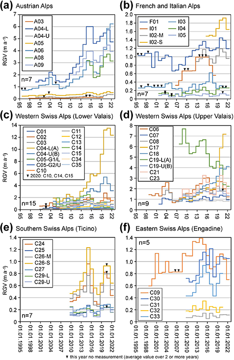
Figure 5. Horizontal RGV since 1995 of 50 timeseries related to 50 RG units in the Alps, divided into seven regions (French and Italian RGs are combine). For abbreviations of the site names see tables 1 and 2. Note the different scale of the ordinate axis. For graphical reasons, an identical field campaign date (15.08.) was used in the graphs for all RGs. For data see appendix.
Download figure:
Standard image High-resolution image4.2. Relative rock glacier velocities
RGV relative to the reference period 2016–2018 are depicted in figure 6. Most RGs in Austria have a consistent movement pattern. A notable exception to this is A06/Äußeres-Hochebenkar, where mean movement in 2021/22 has almost tripled since 2016–2018 (+187%, figure 6(a)) related to destabilization. The differences between the RGV (including RG frontal advance-data at I03/Napfen) in the French and Italian Alps are much larger compared to the Austrian RGs (figure 6(b)). The west-east distance between F01/Laurichard and I03/Napfen is about 500 km compared to Austria with only 180 km. I01/Lazaun is another challenging case due to data gaps. However, a similar movement pattern is still evident for F01 and the two data series at I02/Gran-Sometta (i.e, the westernmost RG in Italy) for the time period 2012–2022. Two distinct time intervals of higher RGV occurred around 2014/15 and 2019–2021 with lower RGV in 2017/18. An even earlier peak of the RGV was notable in 2002–2004. Abrupt decelerations occurred after the 2004- and 2015-peaks followed each time by more gentle and longer acceleration periods. The average movement pattern of all observed French and Italian RGs seems—despite the huge area covered—to be approximately the same as that of the Austrian RGs.
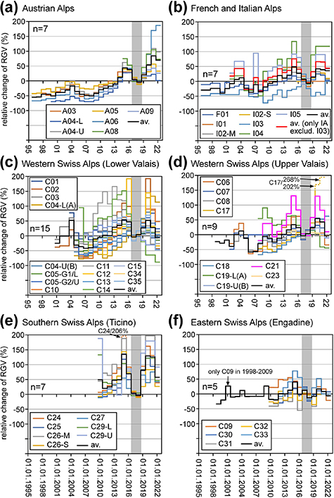
Figure 6. Horizontal RGV relative to the reference period 2016–2018 (grey area) since 1995 of the 50 different RG units in the Alps, divided into seven regions. For abbreviations of site names see tables 1 and 2. The black line represents the average for each region (French and Italian RGs are combined). In addition, in (b) also the Italian average excluding I03 (RG advance monitoring) is depicted.
Download figure:
Standard image High-resolution imageThe 15 RGs attributed to the Lower Valais region (Swiss Alps) are mostly comparable to the other regions discussed so far (figure 6(c)). However, several possible outliers exist such as C01/Aget-Rogneux, C02/Mont-Gelé-B, C11/Lac-des-Vaux-B, C12/Lués-Rares or C14/Tsaté-Moiry-1. C12 reached almost 200% of the average velocity of 2016–2018 in 2015/16. In contrast, C02 accelerated rapidly after 2018 reaching 192% of its former velocity in 2019/20 followed by a rapid decelerating phase afterwards. C14 followed the common pattern before 2016–2018 but decelerated substantially afterwards reaching in 2021/22 only about 10% of the former RGV.
In the Upper Valais several RGs are considered destabilized since the mid-2000s based on satellite interferometry [23]. Three of them are included in this study (C17/Grosse-Grabe, C18/Gugla-Bielzug, C19/Dirru). At C17 and C18 only the respective upper and lower parts are assessed. At C19, a distinction is made between a fast lower (C19-L) and a slow upper (C19-U) part. The nine RG units assigned to this region (figure 6(d)) also show a comparable movement pattern with peaks around 2003/04, 2014/15 and 2019–2021 and lows around 2005–2007, and 2016/17. Distinct differences to this regional pattern were observed at C17. Here, the lower part is destabilized since many years. Whereas the movement had almost stopped, this part of C17 was almost fully covered by the deposits of several large rock falls in summers 2019 and 2020 [81]. The upper part (considered in our study) has destabilized as well since 2020 and no survey has been possible since 2022 because of the rock fall danger. Another 'outlier' is C19/Dirru. Whereas the upper part of this RG (C19-U) follows the average regional pattern, the lower part was very fast particularly in 2008/09, with a second peak in 2013–2015 and has progressively decelerated since then.
RGV monitoring in Ticino started in 2009 [82]. The velocity pattern of the seven RGV based on five different RGs in this region (figure 6(e)) is only partially congruent. At some RGs, the first year of measurement (2009/10) started with higher values (C29-U/Ganoni-di-Schenadüi upper part), others started with very low ones (C27/Piancabella). Most RGs reached distinct peaks in 2014/15 and 2019–2021. The lowest velocities were recorded in 2016–2018 in most cases.
In the Eastern Swiss Alps (figure 6(f)), the movement pattern of the five observed RGs is only moderately comparable with those of other regions of Switzerland and nearby Austria and Italy. In 1998–2009, only one RG was observed (C09/Büz-North) and no surveys were accomplished in 2006 and 2007. All five RGs reached their velocity peaks in 2014–2017: one in 2013/14 (C09), three in 2014/15 (C31/Murtèl-Corvatsch, C32/Marmugnun, C33/Chastelets), and one in 2016/17 (C30/Muragl). A less pronounced second peak occurred in 2019/20 followed by distinct deceleration.
5. Discussion
5.1. Similar behaviour or outlier: where to draw the line?
The averaging of many individual observations for one geomorphic process (e.g. glacier recession; [46]) may help to better understand signals of landscape adaptation to environmental changes. Figure 7 and table 3 combine the mean of each of the six regions. Averaged over all 50 RG units (black curve in figure 7), the following alpine-wide RGV pattern emerged: gentle acceleration phase in 1995–1999, a brief deceleration phase in 1999/2000, a faster acceleration phase until 2003 with a distinct peak in 2003/04 (also observed at other RGs, [83]), followed by a distinct drop of RGV and stable conditions in 2005–2008. This is followed by a general acceleration phase with a second, much higher peak in 2014/15, followed again by a distinct drop of RGV until 2016, stable conditions until 2018, and a last remarkable velocity peak in 2019–2021. In 2021/22 velocities distinctly decreased again.

Figure 7. Regional and total averages of horizontal RGV relative to the reference period 2016–2018 (grey area) since 1995. The number of RGV (maximum per year) for each region is indicated in brackets. I01 (RG advance monitoring) was excluded here from the Italian sample but considered in the total average.
Download figure:
Standard image High-resolution imageTable 3. Averaged RGV relative to the reference period 2016–2018 of the 50 different RG units in the Alps in 1995–2022, divided into the six regions as defined in figure 2 as well as the total average. Values in %. bold and italics = minimum; bold = maximum.
| RGV relative to the mean of 2016–2018 (%) in different monitoring years | ||||||||||||||
|---|---|---|---|---|---|---|---|---|---|---|---|---|---|---|
| Sample (n) | 95/96 | 96/97 | 97/98 | 98/99 | 99/00 | 00/01 | 01/02 | 02/03 | 03/04 | 04/05 | 05/06 | 06/07 | 07/08 | 08/09 |
| Austr. Alps (7) | − 55.0 | −54.2 | −44.9 | −44.8 | −50.9 | −39.2 | −39.0 | −30.9 | −16.9 | −35.5 | −45.1 | −49.6 | −50.8 | −42.4 |
| Fr + Ital. Alps (7) | −29.5 | −29.5 | −23.8 | −23.8 | −40.1 | −24.1 | −7.6 | 6.2 | 12.0 | −23.0 | −37.1 | −11.3 | −35.0 | −18.6 |
| Lower Val. (15) | −25.3 | −0.7 | −0.7 | 52.6 | −31.4 | −36.7 | −42.0 | −40.4 | −10.5 | |||||
| Upper Val. (9) | −23.3 | −28.4 | −18.0 | −39.3 | 0.7 | 12.8 | −11.6 | −58.1 | −56.1 | −29.6 | −5.4 | |||
| Engadine (5) | −33.6 | −20.5 | 26.6 | −10.5 | −8.5 | 11.9 | −8.4 | −7.8 | −7.8 | −7.8 | 26.6 | |||
| Ticino (7) | ||||||||||||||
| All (50) | −52.6 | −52.1 | −43.9 | −38.7 | −43.5 | −28.3 | −21.1 | −8.1 | 12.1 | −27.3 | −39.1 | −37.2 | −38.1 | −13.9 |
| RGV relative to the mean of 2016–2018 (%) in different monitoring years | ||||||||||||||
|---|---|---|---|---|---|---|---|---|---|---|---|---|---|---|
| Sample (n) | 09/10 | 10/11 | 11/12 | 12/13 | 13/14 | 14/15 | 15/16 | 16/17 | 17/18 | 18/19 | 19/20 | 20/21 | 21/22 | |
| Austr. Alps (7) | −29.7 | −24.8 | −17.9 | −10.7 | 12.0 | 43.6 | 38.3 | 4.0 | −4.0 | 20.1 | 53.3 | 84.1 | 69.6 | |
| Fr + Ital. Alps (7) | −7.6 | −1.2 | 19.5 | 11.0 | 20.9 | 49.0 | 27.3 | 6.7 | −6.7 | 14.3 | 42.1 | 39.1 | 35.8 | |
| Lower Val. (15) | −4.8 | 1.7 | 0.8 | 29.0 | 35.4 | 53.3 | 47.2 | −3.9 | 3.9 | 26.4 | 52.6 | 27.6 | −6.3 | |
| Upper Val. (9) | −11.8 | −24.2 | −12.0 | 1.5 | 16.4 | 34.0 | 23.8 | −3.4 | 3.4 | 24.3 | 54.7 | 43.1 | −3.6 | |
| Engadine (5) | −18.0 | −20.1 | 0.8 | 0.4 | 12.6 | 40.1 | −0.4 | 12.7 | −12.7 | −7.7 | 16.9 | 8.7 | −6.4 | |
| Ticino (7) | 48.8 | 20.3 | 25.0 | 47.5 | 48.7 | 135.4 | 69.0 | 3.6 | −3.6 | 81.4 | 129.2 | 125.9 | 57.4 | |
| RGV all (50) | −1.9 | −6.2 | 1.9 | 16.4 | 27.0 | 59.1 | 37.9 | 1.5 | −1.5 | 28.5 | 60.0 | 54.0 | 19.8 | |
The sample size was, however, far from uniform over the time period 1995–2022, varying from less than 10 before 2000 and 50 in the three observation years 2015–2018. RGV of ⩾20 RGs have been available since 2004, >30 since 2007, and >40 since 2009 (figure 8). The longest dataset (excluding RG front-monitoring at I03/Napfen) exists for the Austrian and French Alps, the shortest for Ticino. Taking this data limitation into account, the time period prior to 2009 is more uncertain in terms of an Alpine-wide statement of RGVs.
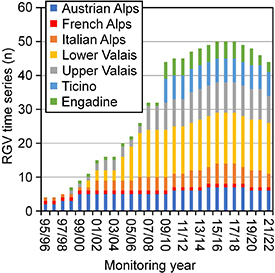
Figure 8. Number of RGV in the time period 1995–2022 in the different regions of the Alps used in this study.
Download figure:
Standard image High-resolution imageSeveral questions arise from this general pattern, such as: How do individual RGV correlate with each other? Which RGs evolve similar to each other, and which ones might be considered as outliers? How do you even define an outlier in this context? Should outliers be used as climate indicators? In addition, a time period with a movement pattern which is congruent to others might transform into a subsequent time interval with outlier behaviour. Finally, what drives these patterns?
Figure 9 summarises the correlations of all 50 RGV based on the relative change of the surface flow velocities using the reference period 2016–2018. This matrix reveals that many RGs correlate well with each other whereas others do not. A total of 584 pairs of values correlate significantly with each other, 23 of which negatively indicating opposite creep behaviour between two RGs. For clarity, a RG with a significant correlation percentage of 50% means that the timeseries of this RG is significantly correlated with half of the other RG in the dataset. A positive correlation indicates that the RGV of two compared RGs is relatively harmonious with each other. A negative correlation indicates an opposite RGV pattern between a pair. Such a pattern might be explained by in-situ permafrost degradation (ice loss, increase of frictional forces) or by topographic conditions. Some RGs moved out of steep slopes onto flatter terrain, resulting in an increase in internal friction and thus deceleration (C11/Lac-des-Vaux and C14/Tsaté-Moiry-1). Finally, two RG that are negatively correlated with most other RGs might, in turn, correlate positively with each other (e.g. C15/Tsaté-Moiry 2 and C19_L/Dirru-lower part). A positive or negative correlation, therefore, also depends on the viewpoint of the observer.
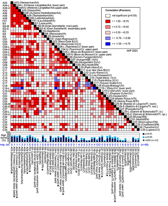
Figure 9. Correlation matrix for all 50 RGV based on the relative change of the surface flow velocities (reference period 2016–2018). Correlations: significant at the <0.05 level. Percentage of significant correlations (distinguished between two levels: p < 0.01, p < 0.05) are additionally shown in the lower graph. 15 RGV (*) have at least 29 significant correlations (i.e. 60%) and form the reduced sample. Number of negative correlations for each RG is indicated.
Download figure:
Standard image High-resolution imageIn figure 9, we used the arbitrary threshold of 60% (i.e. 29 data pairs) of significant correlations as a conservative value to define a non-outlier behaviour (forming the reduced sample). In statistics, an outlier is an observed value that contrasts sharply with the overall pattern of values in a dataset. Therefore, one could argue that the 60% value might be too low or too high but can serve, nevertheless, as a starting point.
All seven RGV in Austria correlate well and positive with each other and many other times series in the dataset. A08/Tschadinhorn has the weakest correlation with 42.9% probably due to the rather short timeseries. The highest correlation degree for Austrian RGs is 75.5% at A05/Dösen. The only French RG considered in our study (F01/Laurichard) is in good agreement with many of the other RGV and yields the highest percentage of significant correlations (77.6%; jointly with two RGV in Switzerland: C05-U/Becs-de-Bosson upper part and C10/Petit-Vélan) of all 50 RGV. None of the Austrian or the French RGV might be considered as 'outlier'.
The correlation result for the timeseries of Italian RGs reveals a complex picture. Only I01/Lazaun (59.2%) and I04/Marocarro (73.5%) correlate significantly with more than half of the other timeseries. Fewer data gaps and fewer averaged multi-annual values at I01 (5 years with annual data, 7 years with averaged multi-annual data) would have presumably resulted in an even higher correlation percentage. The correlation results for three of the six Italian RGV are similar with 37% to 49%. These rather low values are either related to short timeseries (I02-M, I02-S/Gran-Sometta both units) or to a different RGV behaviour or landform origin (I05/Amola; composite permafrost landform formed in glacier-permafrost contact; [41]). The lowest correlation percentage was quantified for I03/Napfen with only 8.2% where frontal advance is monitored.
Of the 36 Swiss RGV, three (C01/Aget-Rogneux, C31/Murtèl-Corvatsch and C32/Marmugnun) correlate significantly with fewer than 10% with the other timeseries. The RGV of these three landforms must be considered as distinct outlier in an Alpine-wide context. C01 is a back-creeping push moraine in continuous degradation and should be excluded from RGV comparisons [56]. The two landforms C31 and C32 are talus-connected RGs but behave differently compared to most others. However, some of their peaks are comparable to other RGs. C31 is very ice rich [84], possibly C32 as well. This could lead to a delayed reaction or a less pronounced one. Thus, reasons for the pattern of C31 and C32 appear to be site-specific effects that overcome the climatic ones. Interestingly, neighbouring C33/Chastelets is in rather good agreement with the Alpine wide signal (55.1% of correlations). The RGV of C31 and C32 should be treated with caution if compared to others.
Between 10 and 30% of significant correlations were quantified for seven Swiss RGV distributed in the Engadine (C09/Büz-North), Lower Valais (C11/Lac-des-Vaux-B, C14/Tsaté-Moiry-1, C15/Tsaté-Moiry-2), Upper Valais (C23/Gruben) and Ticino (one RG with two timeseries—C29-L and C29-U/Ganoni-di-Schenadüi—and low ground temperatures, [65]). While in some cases the unusual creep behaviour may be related to site-specific effects (C09, C11, C14, C15), in others it may be more related to the short timeseries (e.g. C23 since 2012). A site-specific effect was the exceptionally thick and long-lasting snow cover in 2000/01 at C09 accelerating this RG more than the heatwave in 2003. Thus, a possible site-specific effect is a topography favourable—or unfavourable—for snow accumulation.
Between >30% and 60% of significant correlations were revealed for 18 Swiss RGV distributed all over the Swiss Alps (e.g. Engadine: C30/Muragl, C33/Chastelets; Lower Valais: C12/Lués-Rares, C13/Les-Cliosses; Upper Valais: C17/Grosse-Grabe, C18/Gugla-Bielzug; Ticino: C26-M/Stabbio-di-Largario main unit, C27/Piancabella). The 18 RGV in this percentage range can neither be seen as outliers nor as optimal climate indicators. This is partly due to site-specific effects (e.g. unstable front at C18 or C04-L/Tsarmine lower unit; scree slope starting to form RG at C35/Lapires) or possibly also due to data gaps and/or limited length of data series (e.g. C34/Tsavolire).
Finally, eight RGV in Switzerland yield a significant correlation percentage value of >60%. None of the RGs in the Engadine exceed this value. In all other regions in Switzerland the 60%-threshold value is exceeded suggesting an (almost) nation-wide rather homogenous RGV behaviour. Thus, the following Swiss RGV may be considered as the optimal ones for climate-related statements: C21/Grosses-Gufer in the Upper Valais; C02/Mont-Gelé-B, C04-U/Tsarmine upper part, C05-U/Becs-de-Bosson upper part, C10/Petit-Vélan in the Lower Valais, and C24/Monte-Prosa-A, C25/Monte-Prosa-B, and C26-S/Stabbio-di-Largario secondary lobe in Ticino. The timeseries of these eight RGs seem to be the most reliable climate indicators for Switzerland so far. On the Alpine-wide scale, 15 out of the 50 timeseries have at least 60% of correlations between the different value pairs (figure 9). Spatially, these 15 RGs are distributed all over the Alps where active RGs exist, although spatially biased (particularly with CH).
A raster-like analytical approach for the entire Alps considering a certain number of RGs per given area was not feasible in our study as the analysis is restricted to long-term geodetic surveys and related data availability. It is, nevertheless, appropriate that our Alpine-wide RG population might be regarded as representative for the Alps as many RGs (apart from disintegrating ones or other possibly unclear-permafrost landforms) show comparable RGV patterns.
5.2. Environmental response mechanisms: climate, topography, and hydrology
Several environmental parameters influence the creep of the RG permafrost, including gradient of the slope, thickness, temperature, unfrozen water content and water pressure of the creeping frozen body, ice-content, and grain-size of the debris [3, 4, 30]. A comparison of air temperature data (MAAT; here from September to August of the following year) with RGV gives some Alpine-wide insight into RG-thermal aspects. Table 4 depicts a correlation matrix between RGV for different regions, the total sample and the RGV with a correlation percentage >60% (reduced sample) and air temperature (annual and seasonal data). On an annual temperature time scale, significant results (i.e. higher temperatures leading to acceleration and vice-versa) were quantified for only two regions (Austria, Italy) for the total (n = 50) and reduced (n = 15) samples. On a seasonal timescale, only the autumn and the summer temperatures seem to play a significant role in the averaged RGV for some regions but also for the total and reduced samples. At least on an averaged sample scale, the winter and the spring temperatures are of minor relevance for the Alpine-wide RGV pattern. This implies that even on an Alpine-wide, averaged scale, a significant relationship between RGV and air temperature can be established thanks to long-term data and despite a large amount of noise in the data. This confirms the general usability of RGV in an ECV- and thus general environmental context. However, individual behaviour related to site-specific environmental factors such as topographical, ground thermal, and hydrological impacts (the latter two impacted by snow characteristics) potentially influences this general relationship. Care must be taken, therefore, in choosing RGs that might be suitable candidates for RG-climate relationship establishments.
Table 4. Correlation matrix between the different averaged RGV (regional, total, selected) and air temperature (arithmetic mean of Besse, Säntis, Zugspitze, and Sonnblick) distinguishing between mean annual (MAAT; September to August of the following year) and seasonal (SON, DJF, MAM, JJA) values. Only significant correlations (p < 0.05) are shown.
| Air temperature (°C) | |||||
|---|---|---|---|---|---|
| Sample (n) | r for MAAT | r for SON | r for DJF | r for MAM | r for JJA |
| Austrian Alps (7) | 0.51 | 0.39 | ns | ns | 0.48 |
| French Alps (1) | Ns | ns | ns | ns | ns |
| Italian Alps (6) | 0.59 | 0.50 | ns | ns | 0.58 |
| Lower Valais (15) | Ns | ns | ns | ns | ns |
| Upper Valais (9) | Ns | ns | ns | ns | ns |
| Engadine (5) | Ns | ns | ns | ns | ns |
| Ticino (7) | Ns | ns | ns | ns | ns |
| RGV all (50) | 0.46 | 0.44 | ns | ns | 0.40 |
| RGV >60% sig. cor. (15) | 0.46 | 0.39 | ns | ns | 0.47 |
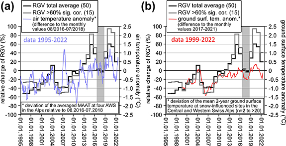
The averaged temperature anomaly (running mean of the 12 previous months) of the four AWS Sonnblick, Zugspitze, Säntis, and Besse (figure 2) and the averaged RGV pattern of all 50 timeseries as well as the 15 timeseries with more than 60% of significant correlations is depicted in figure 10(a). Cold periods distinctly reduced the RGV as in 1999/00, in 2004/05, in 2010/11, in 2015–2017, and in 2021/22. In contrast, the velocity maxima correlate with warm permafrost temperatures as recorded in boreholes at 10 m (e.g. [65]) and are likely a result of the continuously warm conditions in the ground during the last years. This assumption is confirmed by long-term GST data from the Swiss Alps (10b). RGV clearly correlates with the 2-year running mean of GST (M2AGST) at snow-influenced sites in the Central and Western Swiss Alps in 1999–2022 relative to 2017–2021 [29]. Lower ground temperatures seem to be more efficient in RGV deceleration compared to higher temperatures which cause acceleration [28]. Continuous ground and permafrost warming since approximately 2010 caused a general increase in RGV [34].
Figure 10. RGV and temperature: total average of RGV (n = 50) and average of the 15 RGV with more than 60% of significant correlations between data pairs (cf figure 7) relative to the reference period 2016–2018 (grey area) since 1995 and: (a) 12 month running mean of air temperature (MAAT) anomaly relative to 08.2016 to 07.2018 averaged over four AWS (data: Besse, Météo-France; Säntis, MeteoSwiss; Zugspitze, Deutscher Wetterdienst; Sonnblick, GeoSphere Austria) during the time period January 1995 to September 2022 (figure 2 for locations); (b) 2 year running mean of ground surface temperature (M2AGST) at snow-influenced sites in the Central and Western Swiss Alps (n = 2 to >20) in 1999–2022 relative to 2017–2021 (data: Alpine Geomorphology research group, University of Fribourg and PERMOS).
Download figure:
Standard image High-resolution image
The topographic context of the RGs can play a further significant role as for instance the average slope of the landform or if the RG is developing on alternating steep or flat terrain. Such a topographical influence could lead to a significant destabilization of the RG with non-reversible changes [24], which can lead to a split of a RGV of one RG into two datasets assigned to two different RG units. For some RGs, this separation of observations points has been accomplished in the past (e.g. A04, [47]). For others, such a separation will possibly be introduced in the future, with a decorrelating movement pattern of the upper and lower parts (e.g. A06, [49]). For further RGs where such a separation has taken place already earlier, only one unit is surveyed today, partly also due to field safety reasons.
[30] pointed out that interannual and seasonal variability in RG flow cannot be explained by heat conduction alone. Non-conductive processes linked to water availability dominate the short-term variations in velocity. The advection of surface water into the RG and its interaction over porewater pressure with the creep rheology explain the short-term variations in velocity. [85] also concluded that seasonal variations in the flow velocity of Furggwanghorn RG do not depend directly on the temperature at depth but are very likely controlled by hydrological processes (indirectly by temperature). Thus, subsurface water conditions play a further role in RGV [4] but such data are commonly absent at the monitored RGs and the related process understanding is still limited. Recently, [86] observed daily variations in flow velocity on I01/Lazaun relating them to daily variations in discharge, thus, suggesting velocity-control by water at least during summer.
Water (precipitation or meltwater) may infiltrate into the unfrozen sediment layer below the frozen body, increase the hydraulic pressure thus reducing the frictional resistance in the shear horizon, and transports latent heat into the RG. Factors for RG acceleration but also destabilization have been attributed to permafrost degradation caused by environmental changes and feedback mechanisms influencing subsurface water conditions (e.g. [22, 30, 57, 87]). Thus, timeseries of destabilized RG must therefore be carefully considered (e.g. which time period and how intensive was/is a destabilisation phase? [24]), as in our case the ones of (currently) A04/Hinteres-Langtalkar, A06/Äußeres-Hochebenkar, A09/Leibnitzkopf, C04/Tsarmine, C10/Petit-Vélan, C17/Grosse-Grabe, C18/Gugla-Bielzug, and C19/Dirru.
6. Conclusions
The large number of 50 timeseries from 43 RGs in the European Alps allows for a unique in-depth analysis of long-term velocity variations. The absolute RGVs in the Alps in 1995–2022 varied substantially (0.04–6.23 m a−1), but relative changes in velocities are often comparable despite distinct differences in local settings. Gaps in annual timeseries and differences in the date of measurement can reduce the accuracy of RGV.
Averaged over all 50 timeseries, the following pattern emerges: 1995–1999 gentle acceleration; 1999/2000 slight deceleration; 2000–2004 fast acceleration with a distinct velocity peak in 2003/04; 2004–2006 distinct deceleration; 2006–2008 steady velocities; 2008–2015 long acceleration period with a short time interval of weakened acceleration in 2009–2011; 2014/15 distinct velocity peak in the RGV records followed by a drastic drop; 2018–2020 renewed acceleration leading to peak velocities in 2019–2020 comparable to the ones in 2014/15; 2021/22 strong alpine-wide drop of RGV.
Fifteen out of 50 RGV correlate very well with each other (i.e. >60% of significant correlations between the different RGV). These RGs are most suitable to be used to calculate an Alpine-wide average for RGV. The 15 RGV are distributed all over the Alps in Austria (A03/Weissenkar, A04/Hinteres Langtalkar—upper and lower part, A05/Dösen, A09/Leibnitzkopf), France (F01/Laurichard), Italy (I04/Maroccaro) and Switzerland (C02/Mont-Gelé B, C04/Tsarmine—upper part, C05/Becs-de-Bosson—upper part, C10/Petit-Vélan, C21/Grosses Gufer, C24/Monte Prosa A, C25/Monte Prosa B, C26-S/Stabbio di Largario—lobe West). This correlation may change over time as the RGs may evolve differently related to local factors. Even some currently disintegrating RGs (A04, A09, C04) show good correlation with non-disintegrating ones because of only very recent or weak disintegration.
A decelerating trend of a RG unrelated to the general RGV pattern suggests in-situ permafrost degradation (loss of ground ice), whereas strong acceleration relates to destabilization. Local environmental factors such as topography, hydrology, temperature, geometry, and ice content become dominant and the RGV pattern detaches from the regional environmental signal. A more detailed analysis of RGV and hydro-meteorological conditions (including permafrost temperature, active layer thickness, snow characteristics, hydrology) at the 43 RGs was beyond the scope of the paper and should be considered elsewhere.
A major effort of the RG monitoring community should be to secure the long-term recording of at least annual data (like glacier length-change and mass balance measurement programs) for particularly highly correlating RGs. A continuation of velocity monitoring at RGs with >30% and 60% of significant correlations (24 timeseries) is also encouraged. RG advance monitoring can provide additional interesting information but must be strictly separated from RGV monitoring.
An optimal candidate for the start of a new RGV program using geodetic surveys could be characterized as follows: (a) talus-connected RG system; (b) mono-unit RG system—simple unit; (c) no signs of destabilisation; (d) gently sloping RG with an overall slope of 20°–40° except the front; (e) evenly inclined longitudinal profile at the RG base and in the pro-RG area reducing the chance of future RG-surface rupture; (f) RG front located at least in the 'mostly in cold conditions' permafrost class of [40]); (g) geodetic observation points site not prone to rock falls and well-distributable over the entire unit; (h) logistically easily accessible if possible.
Acknowledgments
Numerous projects funded by different sources support the long-term monitoring of RGV in the European Alps during the last decades. To avoid any unfairness in the naming of funding agencies, we explicitly do not want to name individual institutions but prefer to say a big thank to the various regional, national, and European-wide research funding bodies. One crucial exception to this is, nevertheless, the comprehensive long-term funding of the PERMOS network in Switzerland, supported by MeteoSwiss in the framework of GCOS Switzerland, the Federal Office for the Environment and the Swiss Academy of Sciences. Finally, the authors acknowledge also the financial support by the University of Graz.
Data availability statement
All data that support the findings of this study are included within the article (and any supplementary files).
Author contributions
The original idea of combining the Alpine-wide annual geodetic data was developed in the mid-2000s by several people in central Europe around IGR [35] and RD [36]. Some 10 years later, AKP, together with CL, IGR, RD and XB, took up this idea again, developed it further and coordinated it for this paper. AKP coordinated the content of the paper, compiled, homogenised, and processed the different data, performed most of the analyses, wrote the initial manuscript and designed the figures including the map with contributions of XB, BD, RD, JE, GR, AI, VK, CL, RS, CS, MSW and ET. Almost all the 23 authors carried out field work and data collection. Finally, all the authors contributed to improve the first draft of the manuscript.
Supplementary data (<0.1 MB XLSX)