An Empirical Model for Rainfall Maximums Conditioned to Tropospheric Water Vapor Over the Eastern Pacific Ocean

Introduction

Disasters produced by extreme, episodic, and abrupt rain events are still the deadliest natural hazard globally, with the most destructive and long-term effects on the economy, infrastructure, ecosystems, food security, and people (Jonkman, 2005; Pielke et al., 2013; Ilbay-Yupa et al., 2019; Li et al., 2019). This vulnerability not only reflects the importance of adequate population spatial planning but also the low accuracy of Numerical Weather Prediction (NWP) models in terms of forecasting high rainfall intensity rates for global events, especially in the most vulnerable zones (Schumacher, 2016).

Empirical modeling was proposed as a complementary strategy to improve rainfall modeling and prediction capabilities in NWP models (Jakob Themeßl et al., 2011). It relates to observed meteorological variables in new relationships, improving rain estimations or even providing indications of new physical implications of rainfall. Empirical relationships could be used to estimate rainfall over orographically stepped zones in order to address shortcomings with NWP models (Haiden and Kahlig, 1994; Vuille et al., 2000; Buytaert et al., 2006; Villacís et al., 2008; Junquas et al., 2018; Padrón et al., 2020), by improving the location of rain events (Herman and Schumacher, 2016) and improving the quantification of high-intensity rain events.

Over the ocean, temperature and atmospheric humidity have empirical relationships with rainfall (Bretherton et al., 2004; Holloway and Neelin, 2009; Nathan et al., 2016; Takahashi and Dewitte, 2016; Ahmed and Neelin, 2018). The positive relationship between sea surface temperature (SST) and rain intensities has been widely reported (Manabe et al., 1974; Johnson and Xie, 2010; Jauregui and Takahashi, 2018) mainly due to the increase in parcel instability and the convective available potential energy (CAPE), which makes it possible to overcome the convective inhibition (Betts and Ridgway, 1989). Additionally, using monthly data, the observations show a rainfall peak between SST values of 26 and 28°C; this temperature range was identified as a convection trigger by several authors, and after this SST maximum, the rain intensities decrease (Gray, 1998; Johnson and Xie, 2010; Vincent et al., 2012; Jauregui and Takahashi, 2018).

With regards to the relationships with humidity, and using a different time resolution, Bretherton et al. (2004) present an exponential dependence between the daily mean precipitation and the column-relative humidity [obtained by dividing the total precipitable water (TPW) by its corresponding saturation value]. TPW represents the depth of water in mm in a column of the atmosphere in the case that the water in that column was precipitated as rain. This study was conducted over four oceans and 4 years, and using satellite data with a resolution of 2.5°× 2.5° (279.3 × 279.3 km).

In a similar study carried out with a temporal resolution of 3 h and a spatial resolution of 0.25°× 0.25° (27.9 km × 27.9 km), Peters and Neelin (2006) reported a power law relationship between the mean rainfall and TPW, exceeding the critical value of TPW. In other research with a similar resolution, rainfall and TPW values were reported (Schroeder et al., 2016; Kuo et al., 2017) when studying tropical convection over the ocean at different pressure levels (Neelin et al., 2009), and even over land (Bernstein and Neelin, 2016; Leon et al., 2016; Sapucci et al., 2019).

A high temporal and spatial resolution analysis of rainfall could provide more realistic results. If a coarse temporal and spatial resolution is used instead, this could lead to the pooling of small events and the underestimation of large events by averaging them with shorter or null events (Lovejoy and Mandelbrot, 1985; Peters et al., 2002; Dickman, 2003; Newman, 2005). Additionally, an adequate spatial resolution may give a more exact and precise location of the rainy event and its predictors.

One particular difficulty for estimating rainfall rates lies in the statistical features related to maximum rainfall events (Arakawa, 2006). Rainfall occurrence is characterized by numerous small intensity events and only a few heavy intensity events; however, these large events are strongly representative because, depending on the study area, they can discharge 70–90% of the total amount of rain registered in 1 year (Pendergrass, 2018). These large events are not well reproduced by the NWP model and are one of the causes of high vulnerability to extreme rainfall events. Then, the maximum rainfall is of special interest since it indicates the maximum amount that the atmospheric system can precipitate, producing the largest and most destructive rainy events.

Therefore, the objective of this study is to develop a high temporal and spatial resolution analysis of maximum rainfall rates related to TPW and SST. Thus, microwave satellite data from TRMM (Tropical Rainfall Measure Mission) Microwave Imager (TMI) Level 2 Hydrometeor Profile Product (TRMM Product 2A12), with a resolution of 5.1 × 5.1 km and 1.67 s, is used in this research. This data proves to be very useful and provides reliable data over the ocean even during storms and hurricanes. Moreover, its advantages include reliability, broad area coverage, and accessibility where in situ data are scarce (Khairoutdinov and Randall, 2006; Wilcox and Donner, 2007; Wang et al., 2009). The area chosen in our study is in the eastern part of the tropical Pacific Ocean (i.e., the Eastern Pacific Niño, or Niño E region), reported as a heavy rainfall area in which events could affect the surrounding coastal population (Takahashi and Dewitte, 2016).

The aims of this paper are threefold: (i) to perform a statistical evaluation of the rainfall, TPW, and SST, (ii) to determine the point estimate relationships between intense rainfall and its predictors by choosing the most suitable mathematical model able to estimate maximum rainfall by season, and (iii) to spatially analyze the performance of the empirical model with respect to the spatial location of the rainfall event as a study case.

Study Area and Data

Figure 1 presents the Niño E area, an area spanning 560,242 km² (0–5°S and 90–81°W). This area is important due to the presence of heavy rains and the influence of the ENSO (El Niño South Oscillation) phenomenon. It is in the vicinity of the northern South American coast, affecting Ecuadorian and Peruvian territories in particular (Takahashi et al., 2011; Takahashi and Dewitte, 2016).

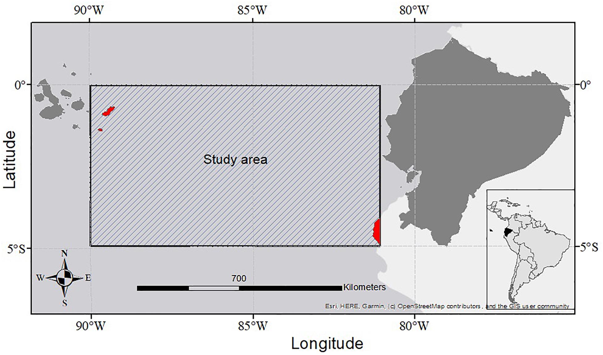
Figure 1. Study area over the eastern equatorial Pacific, called Niño E (Takahashi and Dewitte, 2016). The zones over land (red) are excluded from the study area.

This data comes from a TRMM Microwave Imager (TMI) satellite, which is a passive microwave radiometer and a dual-polarized (vertical and horizontal) multichannel sensor with the following five frequencies: 10.65, 19.35, 37, and 85.5 GHz; the 21.3 GHz frequency has vertical polarization only. The spatial coverage ranges from 40°N to 40°S and the satellite was launched on November 27, 1997, at an altitude of 380 km and an inclination of 35° (NASDA, 2001). Specifically, the 2A12 level has 16 orbits per day with 2,991 scans, each with 280 high-resolution pixels, and a data offering of 5.1 × 5.1 km each and 1.9 s, which is the scan rotation period (Wentz et al., 2001). The satellite swath lasts around 3 min overflying the study area, twice a day, resulting in a non-continuous but randomized time series, hereafter referred to as the Rainfall Intensity Data (RID). This information is available in HDF4 and .nc format at http://disc.sci.gsfc.nasa.gov/precipitation/documentation/TRMM_README/TRMM_2A12_readme.shtm.

The available TMI-TRMM instantaneous RID rates are calculated using the Goddard profiling algorithm (GPROF) (Kummerow et al., 2001), where the response functions of different channels detect different depths within the rain column, defining different brightness temperature vectors Tb, each one related to a vertical distribution of the hydrometeors R. However, the desired variable is the contrary, i.e., the vertical distribution of the hydrometeors R, for a given Tb. Then, in terms of probability, it is estimated by Bayes Eq. 1:

where Pr⁡(R) represents a rain probability observed profile that is determined by CRM (cloud-resolving models). Once the Pr⁡(R)  has  been  reached, the intensity of the rain is derived; this estimation is especially accurate over the ocean (Furuzawa and Nakamura, 2005). In order to focus on the maximum rain rates in this research, the chosen values are higher than 0.1 mm/h (Table 1).

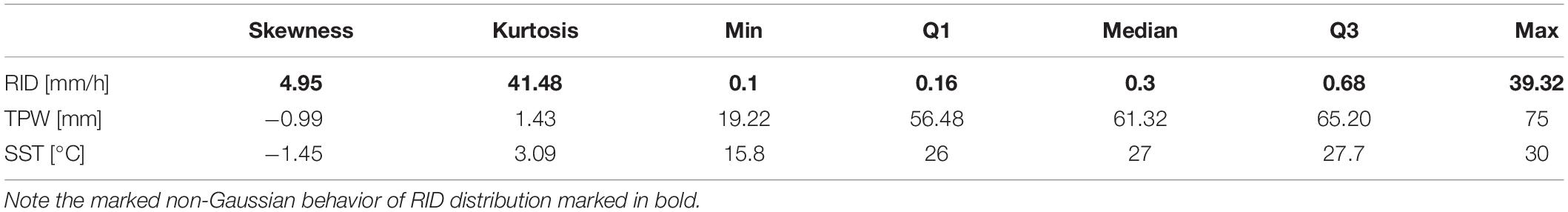
Table 1. RID, TPW, and SST main statistical metrics.

Over the oceans, the GPROF as well as TMI 2A12 product compare well with atoll rain gauge data. The TMI 2A12 rain rate is biased negatively by 9%, and with a correlation of 0.86. The correlation increases to 0.91 and is positively biased by 6% if two or more atolls are used in the validation (Kummerow et al., 1996). The expected sampling errors for the rain estimation are calculated by algorithms and depend on the rain intensity; i.e., the more intense the rainfall the more accurate the TMI estimation, following Eq. 2:

where R is rainfall intensity in mm.h^–1 and σ is its standard deviation. Therefore, TMI 2A12 data are better for determining intense rainfall rates (Olson et al., 1999; Bell et al., 2001).

The amount of TPW detected by TMI that is related to the liquid equivalent of the total water vapor column in mm has its absorption line in the 21.3 GHz band, i.e., it is an accurate measurement due to this high signal-to-noise ratio (Furuzawa and Nakamura, 2005); the root mean square error (RMSE) is 8.1 mm with a bias of −0.76 mm, after radiosonde validation (Sajith et al., 2007). However, this data is only reliable over the ocean, since it overlaps with the terrestrial albedo over land. It is important to mention that CRM ancillary data report few TPW values higher than 70 mm, and this difference could lead to numerical instabilities over this value (Kummerow et al., 2001). Finally, the SST product is estimated directly by using lower bands such as 19.35 and 10.65 GHz and is given in K (NASDA, 2001); thus, the accuracy of the estimation is 0.95 K (Guan and Kawamura, 2004).

Materials and Methods

A statistical analysis of the studied variables (RID, TPW, and SST) is presented in section “P, TPW, and SST Statistical Metrics” to find the model for the maximum rainfall values. In section “Relationships Between Intense Rainfall Rates, TPW and SST,” the relationships of the maximum rainfall values conditioned to TPW (Peters and Neelin, 2006; Neelin et al., 2009) and SST (Jauregui and Takahashi, 2018) were analyzed. Then, the choice of the best model and the confidence intervals were found according to the model selection methodology. Finally, in section “Spatial Analysis,” the predictive performance and location of the model in a case study were analyzed.

P, TPW, and SST Statistical Metrics

First, the data were downloaded and decrypted using Python as detailed in Serrano (2016). Big data post-processing and data selection were performed in R using High-Performance Computing (HPC) MODEMAT at the Escuela Politécnica Nacional laboratory. The chosen data (rain >0.1 mm/h) were 326,092 rain pixels observed over the study area.

Monthly boxplot analyses of the data were performed to determine the seasonality of RID, TPW, and SST. The characteristics of the rainy and dry seasons were identified (Figure 2). Then, a statistical evaluation of RID, TPW, and SST was presented by using frequency histograms (Figure 3). Table 1 shows the main descriptive estimators to determine the normality of the data and its statistical implications.

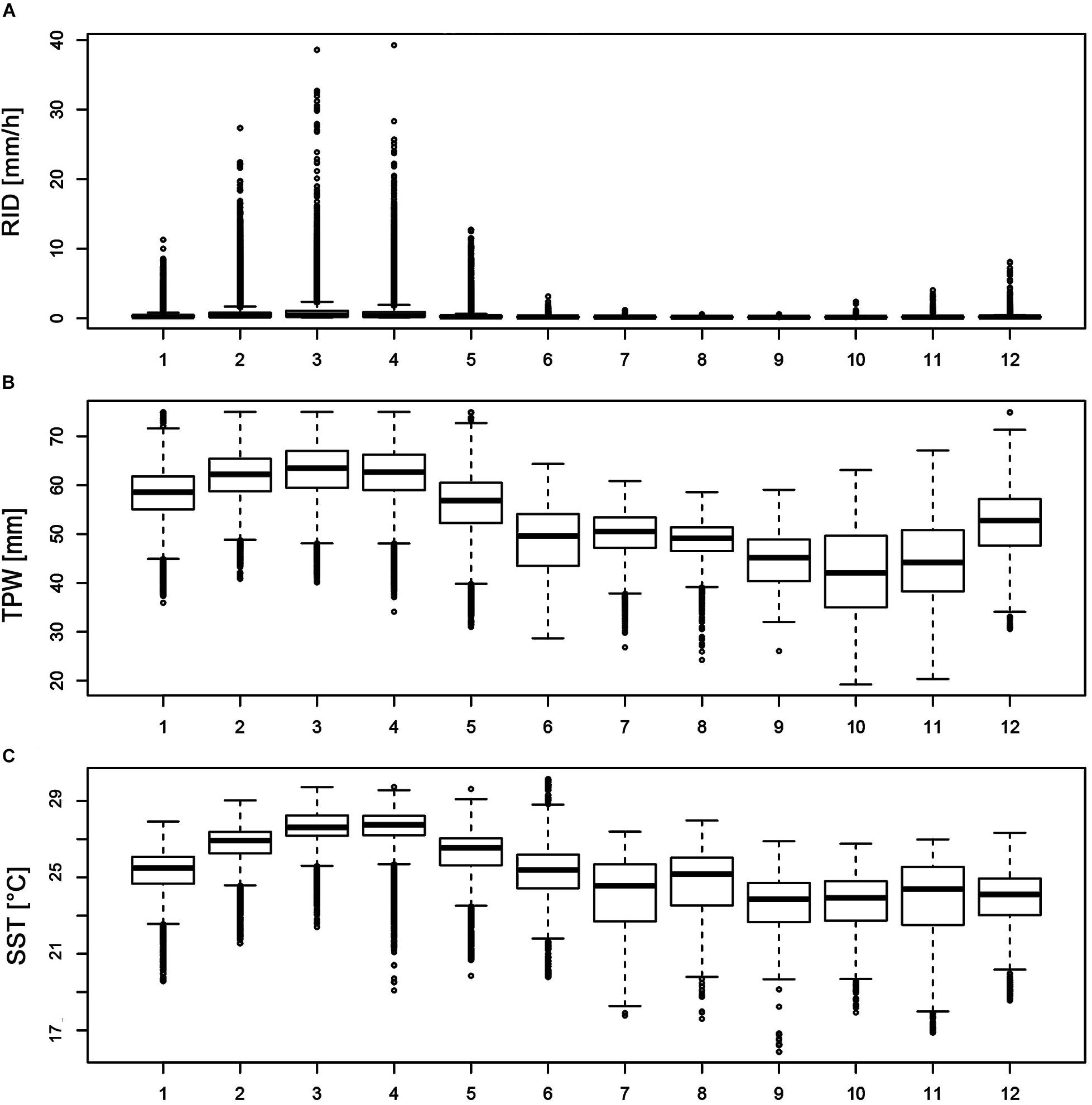
Figure 2. Monthly boxplot analysis for (A) RID, (B) TPW, and (C) SST. The rainy season extends from February to April and the dry season extends from August to October.

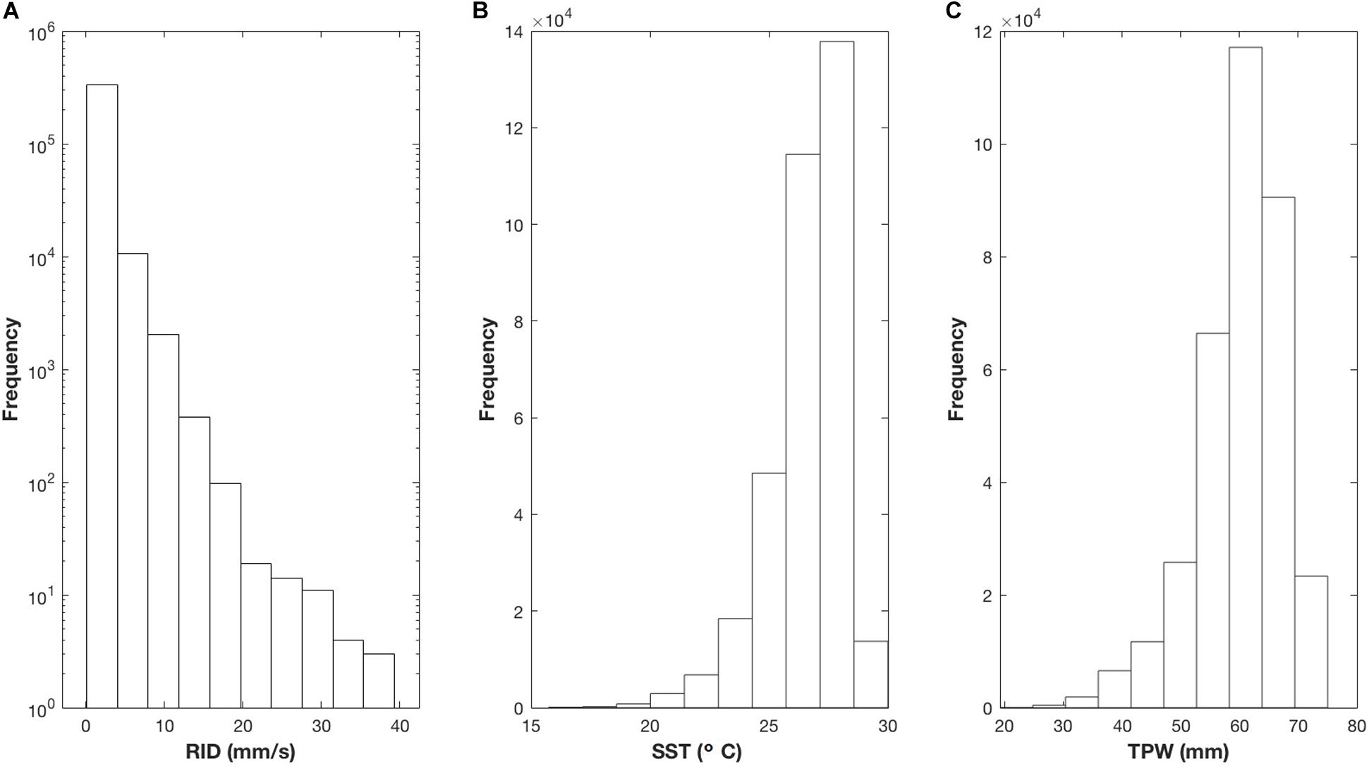
Figure 3. High-resolution data frequency histograms for the studied variables: (A) RID (y-log scale), (B) SST, and (C) TPW from 2009 to 2012.

Relationships Between Intense Rainfall Rates, TPW, and SST

The data were divided into identical 200 bins to determine the dependence of the rainfall rates on TPW and SST. The data were first aggregated into 0.25 mm TPW bins, and then into 0.07°C SST bins. The selected number of bins does not affect the behavior of the studied meteorological variables. The maximum RID values related to each bin were collected and identified with their corresponding SST and TPW values. Based on the scatter plots of the data and the literature, different models were evaluated ranging from exponential (Bretherton et al., 2004), power laws (Peters and Neelin, 2006) and stretched exponential (Martinez-Villalobos and Neelin, 2018), among others.

Distribution fitting was performed using mixed non-linear regression methods in the nls R package (Baty et al., 2015). These methods optimize a modification of the least-squares criterion, which can be applied to non-Gaussian variables. The parameters of the model are estimated iteratively by using starting values. The fit of the non-linear regression is evaluated using graphical tools and the standard confidence intervals are derived, assuming normality in the standard deviations, by obtaining the typical metrics of the residuals. This procedure was repeated for each model: i.e., exponential, power-law, stretched exponential, and polynomial relationships.

The best model was chosen using the standard errors (calculated using the Hessian matrix estimate in the maximum likelihood estimation) as well as the AIC and BIC. The last two criteria estimate the information that a model loses when fitting the data, balancing the underfitting by goodness-of-fit and by using likelihood with the overfitting, due to the unnecessary addition of parameters. Therefore, the model that lost the least amount of information was selected as the best model (Clauset et al., 2009).

Finally, the chosen model was proven in the dry (ASO) and wet season (FMA) separately, repeating the procedure described above, in order to determine the influence of these seasons on the RID data.

Spatial Analysis

A study case (April 5, 2012) is presented to determine the performance of the selected model with regards to rain intensity estimation and spatial location. This event corresponded to the largest rain event registered in the observed satellite swath (lasting 3 min, twice a day, over the study area from 2009 to 2012). A pixel-by-pixel comparison of the RID with TPW and SST was carried out using R raster libraries.

The maximum rainfall pixels were calculated using the model selected in Eq. 3, based on each TPW value, in order to obtain the maximum modeled rainfall. Finally, the differences between the modeled and observed RID values are used to evaluate the performance of the spatial model. This type of spatial analysis will allow to evaluate the performance of the model in the different regions of the cloud, as well as to verify the ability of TPW and SST to locate the maximum rainy events, with low-cost calculations.

Results and Discussion

Monthly Analysis

In the RID, TPW, and SST boxplots presented by month (Figure 2), most of the events have small intensities in both the wet and dry season due to the high resolution of the data. Unimodal seasonality is evident with a marked rainy season from February to April, and a dry season from August to October. This behavior is well known (Manabe et al., 1974) and is mainly due to the influence of the Intertropical Convergence Zone (ITCZ), which is at the southernmost location in March, resulting in low-pressure systems and a marked increase in SST (Jauregui and Takahashi, 2018) favoring convective rainfall in the first part of the year. To the contrary, the ITCZ is at its northern maximum in July–August, decreasing low pressure and precipitation as well (Campozano et al., 2016, 2018). During the dry season, the events are not larger than 1 mm/h, while in the wet season they can reach magnitudes up to 40 times larger, presenting a large seasonal contrast. Similar behavior—but not as marked as that observed for rainfall—is reported for TPW and SST, evidencing their direct relationship with precipitation. More evaporation occurs with warmer SST values, and then more warm water vapor over the surface could ascend, increasing the TPW (Wu et al., 2009). This response is related to the Clausius-Clapeyron relation: the warmer the air, the more moisture it can contain; and later it condensates as precipitation (Roderick et al., 2019).

Statistical Evaluation of RID, TPW, and SST

In Figure 3, the frequency histograms for TPW and SST present a Gaussian left-skewed behavior. However, the RID distribution presented on a semi-logarithmic scale shows right skewness and high kurtosis (see Table 1). It is evident that RID follows a non-Gaussian heavy-tailed distribution with Q1, Q2, and Q3 less than 0.68 mm/h, whereas the maximum value is 39.32 mm/h.

Due to its Gaussianity, the best parameters for describing the behavior of TPW and SST were the mean and variance. However, the strong heavy-tailed behavior of RID shows the importance of large values in these data. Maximum events shape rain distributions and need to be analyzed carefully (Clauset et al., 2009).

Functional Relationships Between Rainfall, TPW, and SST

The maximum RID values associated with each TPW and SST bin are presented in Figure 4. These 200 values are hereafter referred to as MRI_TPW for the Maximum Rainfall Intensity conditioned to TPW, and their corresponding TPW and SST values are denoted as TPW_Max and SST_MaxTPW. Similarly, MRI_SST is the Maximum Rainfall Intensity conditioned to SST, and the corresponding TPW and SST are TPW_MaxSST and SST_Max, respectively.

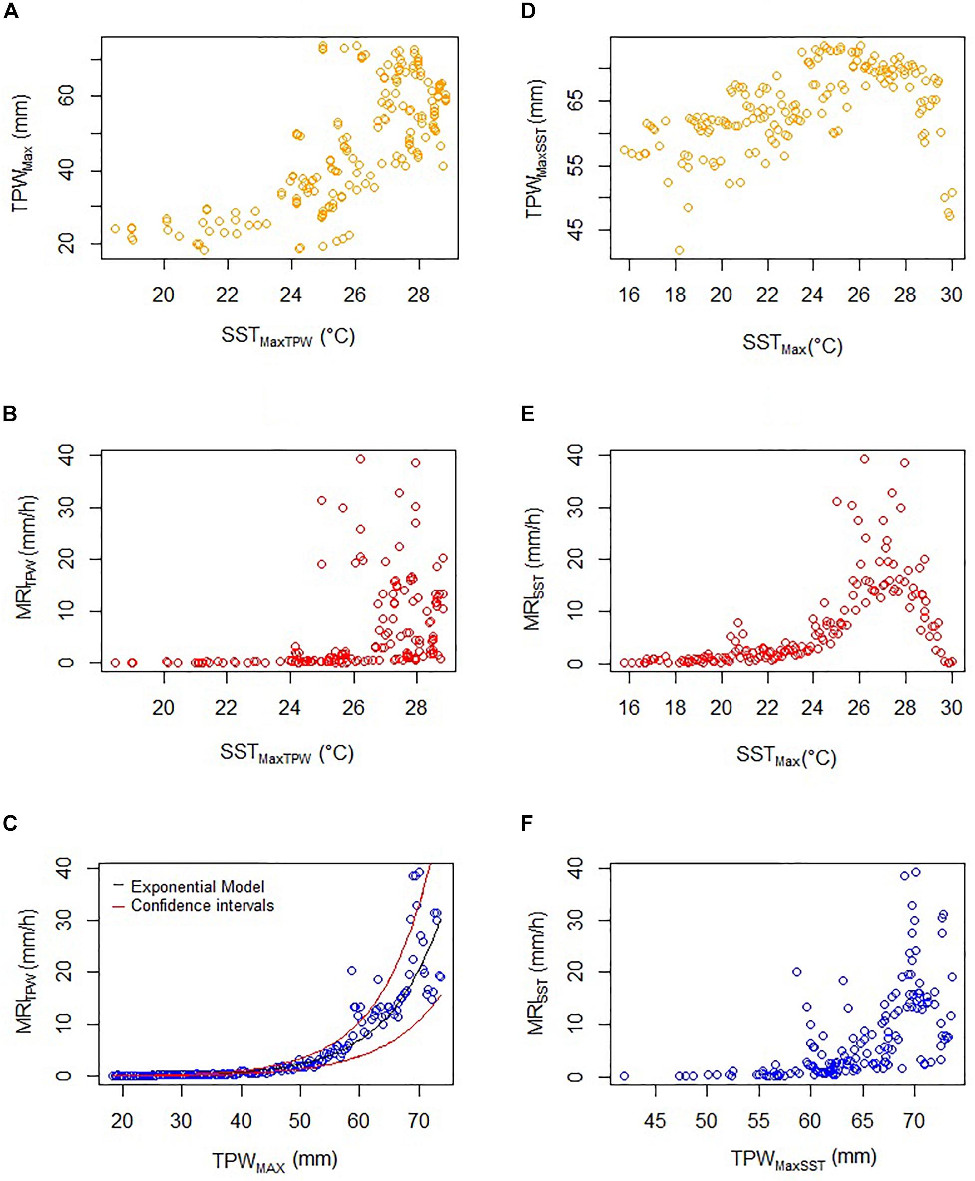
Figure 4. MRI points associated with TPW (left side): (A) TPW_Max vs. SST_MaxTPW; (B) MRI_TPW points and their corresponding SST values (SST_MaxTPW); (C) MRI_TPW associated with the TPW_MAX bins, including the adjusted exponential model selected (continuous black line) and the 95 percent confidence intervals (red lines). Right side: MRI points associated with SST: (D) TPW_MaxSST vs. SST_Max; (E) MRI_SST points and their corresponding SST values (SST_Max); (F) MRI_SST associated with TPW_MaxSST.

The associated TPW_Max vs. SST_MaxTPW values for the 200 MRI_TPW bins are presented in Figure 4A. It shows a positive but scattered dependence: as the SST increases, the TPW content increases as well (Gamache and Houze, 1983). An increase in the slope is presented above 24°C for SST_MaxTPW. Similar behavior is shown in Figure 4B where the maximum rainfall MRI_TPW values and their corresponding SST_MaxTPw values are presented. The same threshold of 24°C marks a phase of higher and more dispersed rain intensity. Below this value, MRI_TPW does not exceed 0.5 mm/h.

The MRI_TPW bins and their corresponding TPW values are presented in Figure 4C. It shows that maximum rainfall increases rapidly with TPW. The rainfall increase related to TPW is smooth and continuous, which points to a rapid growth function. From the findings in the literature, similar studies with 3-hourly mean rainfall values indicate that these suitable models could be exponential (Bretherton et al., 2004), power law (Peters and Neelin, 2006; Neelin et al., 2009) or stretched exponential models (Martinez-Villalobos and Neelin, 2018), among others like potential functions.

The model selection is presented in Table 2. Based on the convergence of the parameters, fitting residuals, and the AIC and BIC information criteria, it is determined that the best model is the exponential model, followed by the power law model.

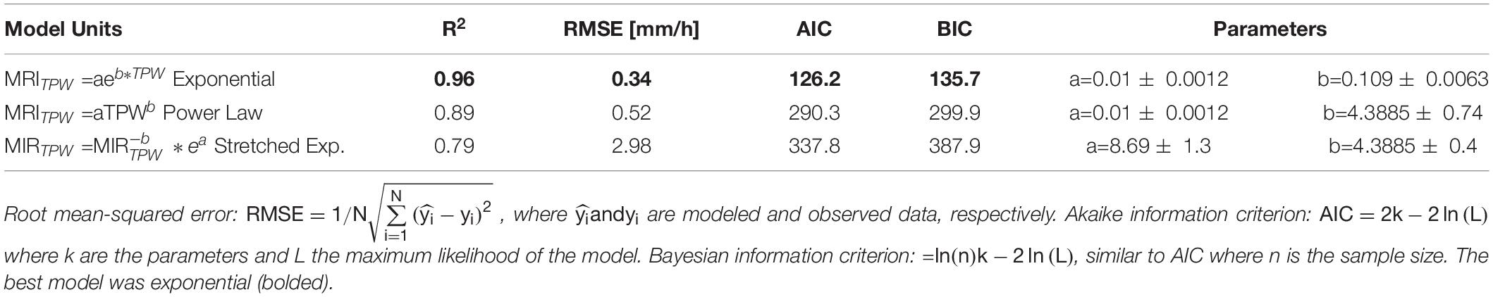
Table 2. Performance measures of model selection between MRI_TPW and TPW: Multiple R-squared error R² =ρ² where ρ is the correlation coefficient.

Then, the rainfall maximum MRI conditioned to TPW follows an exponential model (Eq. 3):

It shows that the model performs well for the maximum rainfall values, and only the highest values are underestimated. This behavior could be due to two reasons: first, the proximity to the 70 mm threshold, where the scarcity of the CRM data needed for the rain satellite calculation could result in artificial numerical instability effects as mentioned in section “Materials and Methods” (Kummerow et al., 2001). The second reason could be due to the highest rain values, which could correspond to a reinforced convection typical of the center of the storm. The predictability of convection events is limited due to turbulence complexity (Nielsen and Schumacher, 2016). Therefore, it is important for future research to determine if this value of 70 mm represents an artificial threshold or a physical one.

Scattered relationships are presented for the MRI data associated with the SST values (right side of Figure 4). First, in Figure 4A, the TPW vs. SST plot for the maximum values related to SST are presented. The data presented a mild threshold between 26 and 28°C, similarly to Figure 4B, where the reported threshold of 26–28°C for the rainfall peaks is presented (Gray, 1998; Johnson and Xie, 2010; Jauregui and Takahashi, 2018). In this study the peak coincides although the time scale used in the literature is monthly.

Due to the great thermal inertia of the water, and consequently of SST, the increase over 26°C is due to the climatological presence of ITCZ, which results in general warming and, therefore, the arrival of the rainy season (Figure 2C). In other words, SST serves to characterize rain behavior on a climatic scale, rather than to characterize specific events of rainy precipitation. In section “Spatial Relationships,” the low localization capacity of SST can be seen in a case study (Figure 6B). Therefore, SST is not a suitable variable in terms of proposing a functional model for rainfall. Finally, Figure 4F presents the rainfall MRIss_T points and their corresponding TPW_MaxTPW values. Over 60 mm of TPW indicate a high rainfall intensity, but in a very scattered manner.

Figure 5 presents the above analysis for the wet and dry season separately. Including the TPW and SST values registered in each season. The events that appear most in the model correspond to opposite seasons, i.e., the driest (ASO) and wettest (FMA) seasons (Figure 5A). This result is remarkable because the exponential model represents the absolute opposite seasons instead of the intermediate—and most frequent—seasons. Most of the maximum rain rates associated with the TPW values belong to the wet season, as expected, however, the smallest maxima have small TPW values (<34 mm), which are only present in the dry season (Figure 5B). And its intensity does not exceed 1 mm/h over the entire range. This fact proves that the model can be applied over the entire range of the rainfall and TPW values.

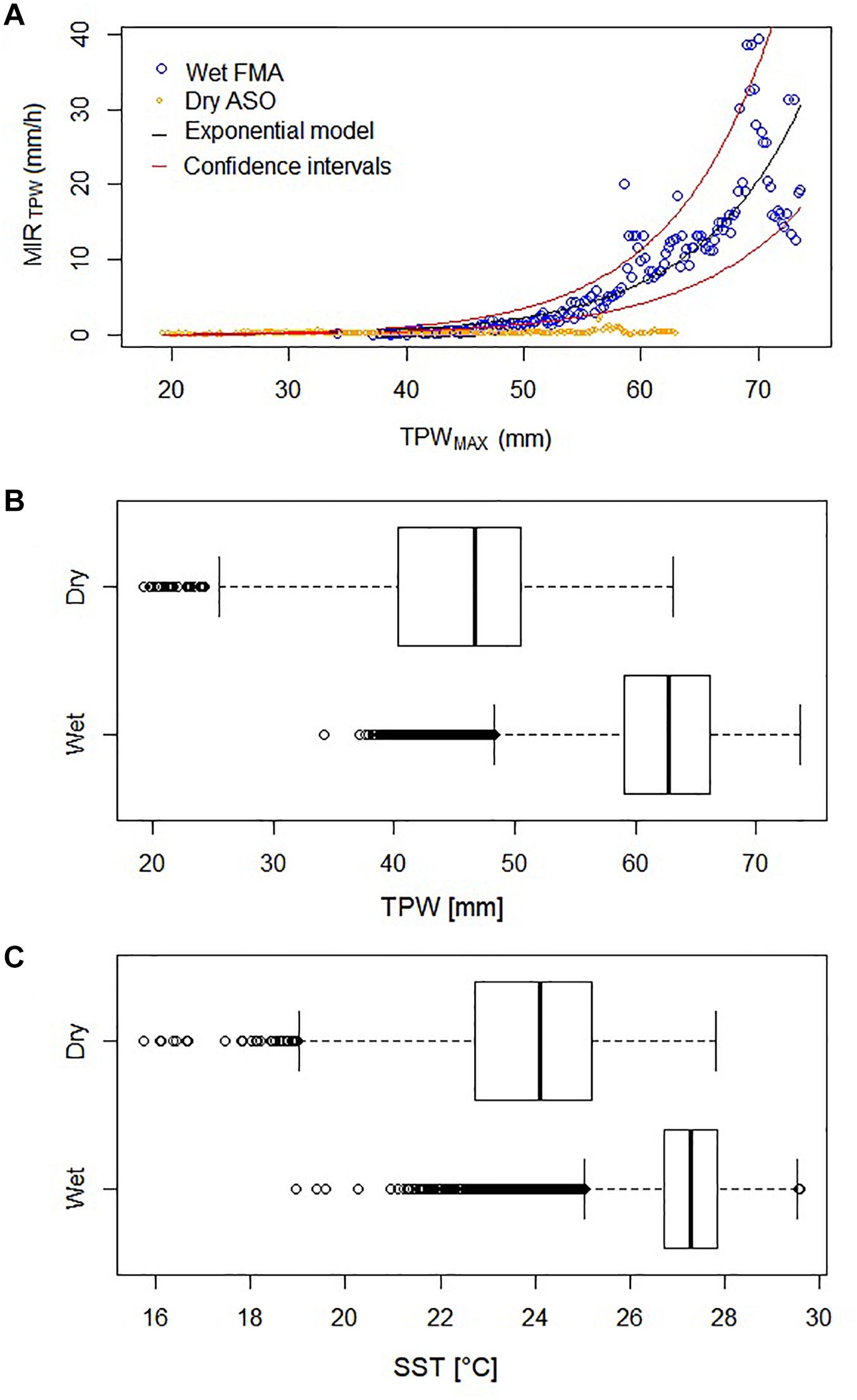
Figure 5. (A) MRI values for the wet and dry seasons, separately, associated with the TPW values. The adjusted exponential model and its confidence intervals are presented; (B) TPW values of the Dry and Wet season; (C) SST values registered in the Dry and Wet season.

Seasonality is also marked when analyzing SST (Figure 5C); in the wet season, the majority of events are between 26 and 28°C. As mentioned before, it is a region with high rainfall rates.

Spatial Relationships

Figure 6 shows the spatial distribution of the studied variables in the study case of April 5, 2012, from 8:50 a.m. to 8:53 a.m. In the spatial analysis, a comparison between RID, SST, TPW, the model estimation, and the difference between the observed and modeled data are presented.

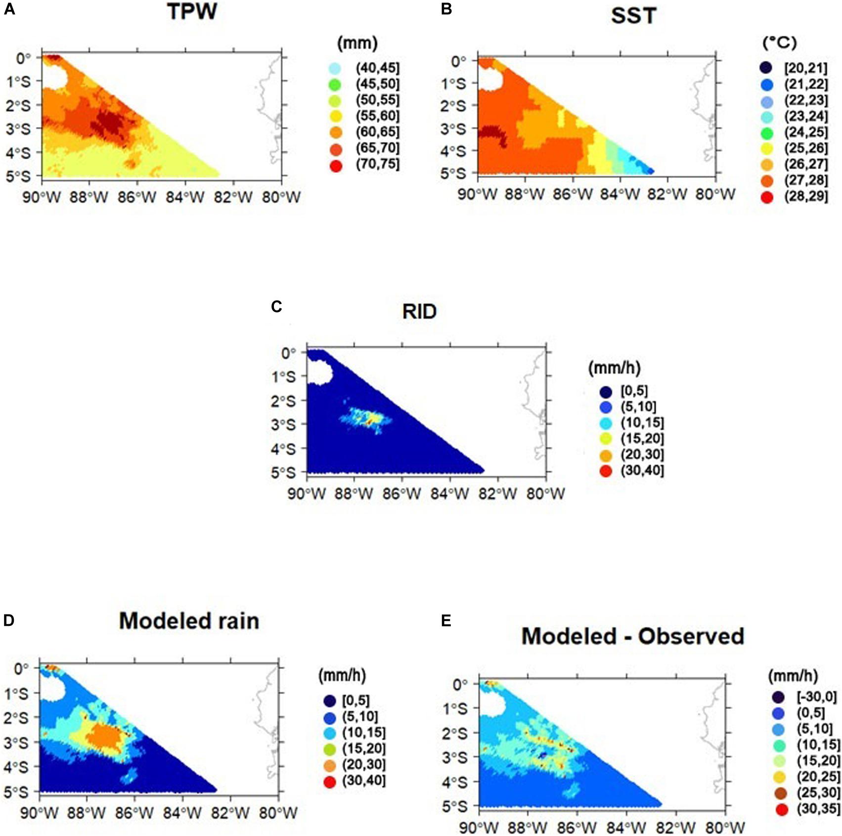
Figure 6. Graphical representation of the satellite scan over the study area on April 5, 2012, from 8:50 a.m. to 8:53 a.m. The variable analyzed for this rainfall event are (A) TPW, (B) SST, (C) RID, (D) maximum rainfall modeled by the exponential model, and (E) difference between the modeled and observed rainfall.

The first observations indicate that TPW (Figure 6A) is able to locate the rain event but not SST (Figure 6B) which has a more uniform behavior that is primarily influenced by cold coastal upwelling than by the rain event. Furthermore, it is noticed that SST experiences a decrease in the area beneath the rain event. Three main processes could control this decrease in SST under the rain event—oceanic vertical mixing, air-sea latent heat exchange, and advection—all of which are mainly influenced by the convective winds produced by the storm (Vincent et al., 2012). As mentioned previously in section “Functional Relationships Between Rainfall, TPW and SST,” SST is influenced more by seasonal variability than by specific rain events.

Figure 6C shows the RID data, Figure 6D presents the maximum modeled rain using the exponential model (Eq. 3), and Figure 6E depicts the modeled rain minus the observed RID. Two aspects are evident from this figure: first, the model is able to determine the proper location of the rain event, and second, this exponential model overestimates rain events in the surrounding advective zone because the model describes the maximum rain events related to TPW; however, there could be smaller rain events which correspond to the same amount of TPW. The development of a rain process does not depend solely on the amount of TPW. Other dynamic and physical variables must be considered, such as winds, convection, and variations in the CAPE (Convective Available Potential Energy). If all of the weather conditions are well combined, heavy rain will develop, but its intensity will be limited exponentially by the amount of TPW in the area.

All of the MRI values associated with TPW >55 mm were analyzed. Each MRI occurred in 23 rainfall separated events for a total of 29,353 RID (several MRI_TPW events correspond to the same rainfall event). In order to quantify the performance of the model, RMSE and the difference between the modeled and observed rainfall are calculated and presented as a histogram and the associated boxplot (Figure 7).

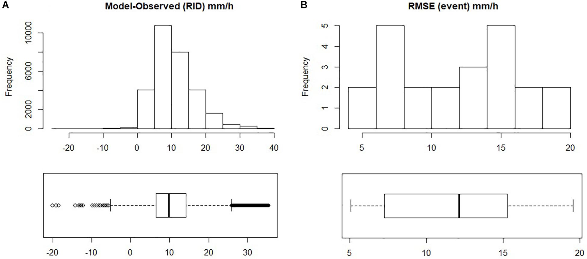
Figure 7. (A) Histogram and boxplot of the differences between the maximum modeled rainfall and observed rainfall using 29,353 RID data. The positive values represent an overestimation (correct model). The negative data represent an underestimation (incorrect model) by 0.4%. (B) Histogram and boxplot of RMSE for the corresponding 23 rainfall events.

The differences between the modeled and observed rainfall in Figure 7A show only 129 negative values, i.e., 0.4%, and therefore 99.6% of the values correspond to an overestimation, which indicates that the model calculating the maximum rainfall values is performing correctly in case studies, where the meteorological conditions for the maximum rainfall development will not always occur. The mean value of these differences represented by the RMSE and calculated for the 23 rainfall events is 11.8 mm/h, the minimum is 5.1 mm/h, and the maximum is 19.6 mm/h (Figure 7B).

Therefore, the most important issue related to this model is that the amount of TPW determines the maximum (but not the minimum) rainfall that the atmosphere can precipitate exponentially. To the contrary, the center of the storm is characterized by deep convection (Figure 8), and the model underestimates the rain intensity at around 20 mm/h, but over a very small area. Extreme convective rain is present into the nucleus of the storm, principally due to a mass convergence from the areas surrounding the convective area (Gray, 1998). Another factor could be the numerical instabilities around 70 mm of TPW (Kummerow et al., 2001) as mentioned in section “Study Area and Data.”

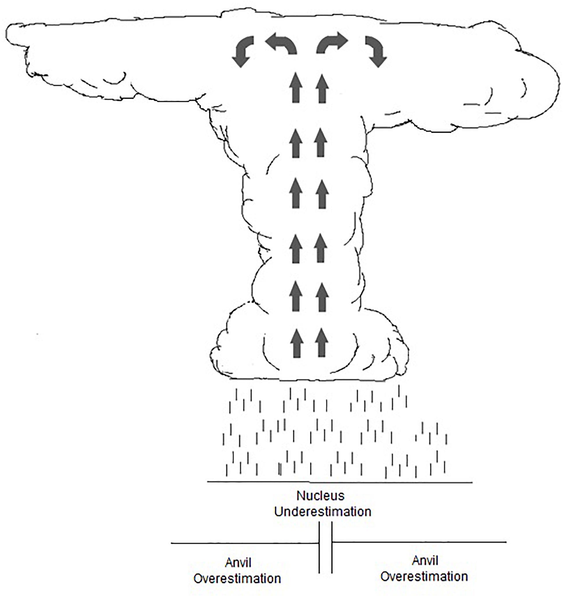
Figure 8. Storm convective cloud diagram, identifying overestimated (nucleus) and underestimated (anvil) areas using the exponential model.

Conclusions

In summary, these results empirically show that the maximum amount of rain that the atmosphere can precipitate depends exponentially on the amount of tropospheric water vapor under the specific geographical conditions of this study. This finding has low computational cost implications for improving heavy rain estimations in terms of the location of the event as well as proposing an upper limit for its intensity.

It is useful to evaluate the risk of a possible extreme event of rain related to a very stable and well-predicted meteorological variable such as TPW. In addition, TPW correctly locates the rain event. However, because it is a model for maximum rainfall, it overestimates the rain in the areas surrounding the cloud, corresponding to the anvil advective area. In contrast, an underestimation was reported in its nucleus, supporting literature findings and the fact that strong convection has its own difficulties in modeling as well as in its prediction due to turbulence complexity (Bellenger et al., 2015).

Finally, it is important to consider the two main limitations in this study. The first is the non-continuity of the collected data, both temporally and spatially, which prevents us from finding cause-effect relationships between TPW and rainfall. The second limitation is the cutoff over 70 mm of TPW; this is due to the lack of base data used to estimate precipitation via satellite by using Eq. 1, which could reproduce non-physical effects over 70 mm. These two limitations can be overcome with future studies on the current topic, using other non-satellite techniques, and obtaining data that allow continuous series in space and time, in order to determine the cause-effect dynamics between TPW and intense rain, as well as over the ocean and land.

There are several techniques to measure TPW with high confidence over land, such as differential absorption LiDAR (Spuler et al., 2015) and atmospheric emitted radiance, among others. However, the most recommended is to estimate TPW via tropospheric delays derived from the Global Positioning System (GPS), which is proportional to the atmospheric TPW content, and can be measured with high accuracy (±2 mm) in all meteorological conditions, at low cost and with high resolution (15 min) (Businger et al., 1996; Walpersdorf et al., 2007; Jade and Vijayan, 2008). The rainfall quantification for a specific studied location would be improved by contrasting these GPS-TPW values with rainfall in situ measurements and by finding empirical relationships between them (Adams et al., 2013; Kuo et al., 2017; Sapucci et al., 2019).

The insights gained from this research may be useful to future studies over land that could be used to prove the relationships found between TPW and intense rain (Eq. 3) and its implications over different climates and orographic conditions. Even so, having reliable TPW data on land could, on its own, improve the forecast of regional mesoscale NWP, where TPW could be adjusted in situ, creating an assimilation process that will improve the forecast modeling in all of the meteorological variables with a low computational cost.

Data Availability Statement

This information is available in HDF4 and .nc format at http://disc.sci.gsfc.nasa.gov/precipitation/documentation/TRMM_README/TRMM_2A12_readme.shtm.

Author Contributions

MV, TC, LC, and SS-V contributed to the conception and design of the study. SS-V organized the database, performed the statistical analysis, and wrote the first draft of the manuscript. SS-V and JG made the maps and graphics. All authors contributed to the article and approved the submitted version.

Funding

Financial support was given by Universidad Politécnica Salesiana doctoral scholarships. The authors also thank the IRD and EPN for the LMI GREATICE grant.

Conflict of Interest

The authors declare that the research was conducted in the absence of any commercial or financial relationships that could be construed as a potential conflict of interest.

Acknowledgments

This research was carried out using the research computing facilities and advisory services offered by the Scientific Computing Laboratory at the Research Center on Mathematical Modeling: MODEMAT, Escuela Politécnica Nacional, Quito, Ecuador. The satellite data was provided by the Goddard Earth Sciences Data and Information Services Center of NASA Goddard Space Flight Center. Additionally, the authors are thankful for the technical support provided by Leandro Robaina. And appreciate the comments made by the reviewers which have greatly enriched this research.

References

Adams, D. K., Seth, I. G., Kirk, L. H., and Dulcineide, S. P. (2013). GNSS observations of deep convective time scales in the Amazon. Geophys. Res. Lett. 40, 2818–2823. doi: 10.1002/grl.50573
Ahmed, F., and Neelin, J. D. (2018). Reverse engineering the tropical precipitation-buoyancy relationship. J. Atmos. Sci. 75, 1587–1608. doi: 10.1175/JAS-D-17-0333.1
Baty, F., Ritz, C., Charles, S., Brutsche, M., Flandrois, J. P., and Delignette-Muller, M. L. (2015). A toolbox for nonlinear regression in R?: the package Nlstools. J. Stat. Softw. 66, 1–21. doi: 10.18637/jss.v066.i05
Bell, T. L., Kundu, P. K., and Kummerow, C. D. (2001). Sampling errors of SSM/I TRMM rainfall averages: comparison with error estimates from surface data and a simple model. J. Appl. Meteorol. 40:956. doi: 10.1175/1520-04502001040<0938:seosia<2.0.co;2
Bellenger, H., Yoneyama, K., Katsumata, M., Nishizawa, T., Yasunaga, K., and Shirooka, R. (2015). Observation of moisture tendencies related to shallow convection. J. Atmos. Sci. 72, 641–659. doi: 10.1175/JAS-D-14-0042.1
Bernstein, D. N., and Neelin, J. D. (2016). Identifying sensitive ranges in global warming precipitation change dependence on convective parameters. Geophys. Res. Lett. 43, 5841–5850. doi: 10.1002/2016GL069022
Betts, A. K., and Ridgway, W. (1989). climatic equilibrium of the atmospheric convective boundary layer over a tropical ocean. J. Atmos. Sci. 46, 2621–2641. doi: 10.1175/1520-04691989046<2621:CEOTAC<2.0.CO;2
Bretherton, C. S., Peters, M. E., and Back, L. E. (2004). Relationships between water vapor path and precipitation over the tropical oceans. J. Clim. 17, 1517–1528. doi: 10.1175/1520-04422004017<1517:RBWVPA<2.0.CO;2
Businger, S., Chiswell, S. R., Bevis, M., Duan, J., Anthes, R. A., Rocken, C., et al. (1996). The promise of GPS in atmospheric monitoring. Bull. Am. Meteorol. Soc. 77, 5–18. doi: 10.1175/1520-04771996077<0005:TPOGIA<2.0.CO;2
Buytaert, W., Rolando, C., Patrick, W., De Bièvre, B., and Guido, W. (2006). Spatial and temporal rainfall variability in mountainous areas: a case study from the south ecuadorian andes. J. Hydrol. 329, 413–421. doi: 10.1016/j.jhydrol.2006.02.031
Campozano, L., Célleri, R., Trachte, K., Bendix, J., and Samaniego, E. (2016). Rainfall and cloud dynamics in the andes: a southern ecuador case study. Adv. Meteorol. 2016, 1–15. doi: 10.1155/2016/3192765
Campozano, L., Trachte, K., Célleri, R., Samaniego, E., Bendix, J., Albuja, C., et al. (2018). Climatology and teleconnections of mesoscale convective systems in an andean basin in southern ecuador: the case of the paute basin. Adv. Meteorol. 2018, 1–13. doi: 10.1155/2018/4259191
Clauset, A., Cosma, R. S., and Newman, M. E. J. (2009). Power-law distributions in empirical data. SIAM Rev. 51, 661–703. doi: 10.1137/070710111
Dickman, R. (2003). Rain, power laws, and advection. Phys. Rev. Lett. 90:108701. doi: 10.1103/PhysRevLett.90.108701
Furuzawa, F., and Nakamura, K. (2005). Differences of rainfall estimates over land by tropical rainfall measuring mission (TRMM) precipitation radar (PR) and TRMM microwave imager (TMI)–dependence on storm height. J. Appl. Meteorol. 44, 367–383. doi: 10.1175/JAM-2200.1
Gamache, J. F., and Houze, R. A. (1983). Water budget of a mesoscale convective system in the tropics. J. Atmos. Sci. 40, 1835–1850. doi: 10.1175/1520-04691983040<1835:WBOAMC<2.0.CO;2
Gray, W. M. (1998). The formation of tropical cyclones. Meteorol. Atmos. Phys. 67, 37–69. doi: 10.1007/BF01277501
Guan, L., and Kawamura, H. (2004). Merging satellite infrared and microwave SSTs: methodology and evaluation of the new SST. J. Oceanogr. 60, 905–912. doi: 10.1007/s10872-005-5782-5
Haiden, T., and Kahlig, P. (1994). Modelling extreme precipitation events. Österreichische Wasser- Und Abfallwirtschaft 46, 57–65.
Herman, G. R., and Schumacher, R. S. (2016). Extreme precipitation in models: an evaluation. Weather Forecast. 31, 1853–1879. doi: 10.1175/WAF-D-16-0093.1
Holloway, C. E., and Neelin, J. D. (2009). Moisture vertical structure, column water vapor, and tropical deep convection. J. Atmos. Sci. 66, 1665–1683. doi: 10.1175/2008JAS2806.1
Ilbay-Yupa, M., Zubieta, B. R., and Lavado-Casimiro, W. (2019). Regionalización de la precipitación, su agresividad y concentración en la Cuenca del río Guayas, Ecuador. La Granja Rev. de Ciencias de la Vida 30, 57–76.
Jade, S., and Vijayan, M. S. M. (2008). GPS-based atmospheric precipitable water vapor estimation using meteorological parameters interpolated from NCEP global reanalysis data. J. Geophys. Res. Atmos. 113, 1–12. doi: 10.1029/2007JD008758
Jakob Themeßl, M., Gobiet, A., and Leuprecht, A. (2011). Empirical-statistical downscaling and error correction of daily precipitation from regional climate models. Int. J. Climatol. 31, 1530–1544. doi: 10.1002/joc.2168
Jauregui, Y. R., and Takahashi, K. (2018). Simple physical-empirical model of the precipitation distribution based on a tropical sea surface temperature threshold and the effects of climate change. Clim. Dyn. 50, 2217–2237. doi: 10.1007/s00382-017-3745-3
Johnson, N. C., and Xie, S. P. (2010). Changes in the sea surface temperature threshold for tropical convection. Nat. Geosci. 3, 842–845. doi: 10.1038/ngeo1008
Jonkman, S. N. (2005). Global perspectives on loss of human life caused by floods. Nat. Hazard. 34, 151–175. doi: 10.1007/s11069-004-8891-3
Junquas, C., Takahashi, K., Condom, T., Espinoza, J. C., Chavez, S., Sicart, J. E., et al. (2018). Understanding the influence of orography on the precipitation diurnal cycle and the associated atmospheric processes in the central andes. Clim. Dyn. 50, 3995–4017. doi: 10.1007/s00382-017-3858-8
Khairoutdinov, M., and Randall, D. (2006). High-resolution simulation of shallow-to-deep convection transition over land. J. Atmos. Sci. 63, 3421–3436. doi: 10.1175/JAS3810.1
Kummerow, C., Hong, Y., Olson, W. S., Yang, S., Adler, R. F., McCollum, J., et al. (2001). The evolution of the goddard profiling algorithm (GPROF) for rainfall estimation from passive microwave sensors. J. Appl. Meteorol. 40, 1801–1820. doi: 10.1175/1520-04502001040<1801:TEOTGP<2.0.CO;2
Kummerow, C., Olson, W. S., and Giglio, L. (1996). A simplified scheme for obtaining precipitation and vertical hvdrometeor profiles from passive microwave sensors. IEEE Trans. Geosci. Remote Sens. 34, 1213–1232.
Kuo, Y. H., Neelin, J. D., and Mechoso, C. R. (2017). Tropical convective transition statistics and causality in the water vapor – precipitation relation. J. Atmos. Sci. 74, 915–931. doi: 10.1175/JAS-D-16-0182.1
Leon, D. C., French, J. R., Lasher-Trapp, S., Blyth, A. M., Abel, S. J., Ballard, S., et al. (2016). The convective precipitation experiment (COPE): investigating the origins of heavy precipitation in the southwestern united kingdom. Bull. Am. Meteor. Soc. 97, 1003–1020.
Li, Y., Guan, K., Schnitkey, G. D., DeLucia, E., and Peng, B. (2019). Excessive rainfall leads to maize yield loss of a comparable magnitude to extreme drought in the United States. Glob. Chang. Biol. 25, 2325–2337. doi: 10.1111/gcb.14628
Lovejoy, S., and Mandelbrot, B. B. (1985). Fractal properties of rain, and a fractal model. Tellus A 37, 209–232. doi: 10.1111/j.1600-0870.1985.tb00423.x
Manabe, S., Han, D., and Holloway, J. (1974). The seasonal variation of the tropical circulation as simulated by a global model of the atmosphere. J. Atmos. Sci. 31, 43–83.
Martinez-Villalobos, C., and Neelin, J. D. (2018). Shifts in precipitation accumulation extremes during the warm season over the United States. Geophys. Res. Lett. 45, 8586–8595. doi: 10.1029/2018GL078465
Nathan, R., Jordan, P., Scorah, M., Lang, S., Kuczera, G., Schaefer, M., et al. (2016). Estimating the exceedance probability of extreme rainfalls up to the probable maximum precipitation. J. Hydrol. 543, 706–720. doi: 10.1016/j.jhydrol.2016.10.044
Neelin, J. D., Peters, O., and Hales, K. (2009). The transition to strong convection. J. Atmos. Sci. 66, 2367–2384. doi: 10.1175/2009JAS2962.1
Newman, M. E. J. (2005). Power laws, pareto distributions and Zipf’s law. Contemp. Phys. 46, 323–351. doi: 10.1080/00107510500052444
Nielsen, E. R., and Schumacher, R. S. (2016). Using convection-allowing ensembles to understand the predictability of an extreme rainfall event. Mon. Wea. Rev. 144, 3651–3676.
Olson, W. S., Kummerow, C. D., Hong, Y., and Tao, W. K. (1999). Atmospheric latent heating distributions in the tropics derived from satellite passive microwave radiometer measurements. J. Appl. Meteorol. 38, 633–664. doi: 10.1175/1520-04501999038<0633:ALHDIT<2.0.CO;2
Padrón, R. S., Feyen, J., Córdova, M., Crespo, P., and Célleri, R. (2020). Comparación entre pluviómetros cuantifica diferencias en el monitoreo de la precipitación. La Granja Rev. de Ciencias de la Vida 31, 7–20. doi: 10.17163/lgr.n31.2020.01
Pendergrass, A. G. (2018). What precipitation is extreme? Science 360, 1072–1073. doi: 10.1126/science.aat1871
Peters, O., Hertlein, C., Christensen, K., and Hertlein, C. (2002). A complexity view of rainfall. Phys. Rev. Lett. 88:4. doi: 10.1103/PhysRevLett.88.018701
Peters, O., and Neelin, J. D. (2006). Critical phenomena in atmospheric precipitation. Nat. Phys. 2, 393–396. doi: 10.1038/nphys314
Pielke, R. A. Sr., Wilby, R., Niyogi, D., Hossain, F., Dairuku, K., Adegoke, J., et al. (2013). “Dealing with complexity and extreme events using a bottom-up, resource-based vulnerability perspective,” in Extreme Events and Natural Hazards: The Complexity Perspective, eds A. S. Sharma, A. Bunde, V. P. Dimri, and D. N. Baker (Washington, DC: American Geophysical Union), 345–359. doi: 10.1029/2011GM001086
Roderick, T. P., Wasko, C., and Sharma, A. (2019). Atmospheric moisture measurements explain increases in tropical rainfall extremes. Geophys. Res. Lett. 46, 1375–1382. doi: 10.1029/2018GL080833
Sajith, V., Adegoke, J. O., Raghavan, S. K., Ram Mohan, H. S., Kumar, V., and Preenu, P. N. (2007). Evaluation of daily and diurnal signals of total precipitable water (TPW) over the Indian Ocean based on TMI retrieved 3-day composite estimates and radiosonde data. Int. J. Climatol. 27, 761–770. doi: 10.1002/joc
Sapucci, L. F., Machado, L. A., de Souza, E. M., and Campos, T. B. (2019). Global positioning system precipitable water vapour (GPS-PWV) jumps before intense rain events: a potential application to nowcasting. Meteorol. Appl. 26, 49–63. doi: 10.1002/met.1735
Schroeder, A., Basara, J., Shepherd, M., and Nelson, S. (2016). Insights into atmospheric contributors to urban flash flooding across the united states using an analysis of rawinsonde data and associated calculated parameters. J. Appl. Meteorol. Climatol. 55, 313–323.
Schumacher, R. (2016). Heavy rainfall and flash flooding. Nat. Hazard Sci. 1, 1–41. doi: 10.1093/acrefore/9780199389407.013.132
Serrano, S. (2016). Fenómenos Críticos En Datos De Precipitación Lluviosa Intensa Detectados Con Radar Y Microondas, En La Zona De Influencia Del Fenómeno Del Niño Sobre El Ecuador. Quito: Escuela Politécnica Nacional.
Spuler, S. M., Repasky, K. S., Morley, B., Moen, D., Hayman, M., and Nehrir, A. R. (2015). Field-deployable diode-laser-based differential absorption lidar (dial) for profiling water vapor. Atmos. Meas. Tech. 8, 1073–1087.
Takahashi, K., and Dewitte, B. (2016). Strong and moderate nonlinear El Niño regimes. Clim. Dyn. 46, 1627–1645. doi: 10.1007/s00382-015-2665-3
Takahashi, K., Montecinos, A., Goubanova, K., and Dewitte, B. (2011). ENSO regimes: reinterpreting the canonical and modoki El Nio. Geophys. Res. Lett. 38, 1–5. doi: 10.1029/2011GL047364
Villacís, M., Françoise, V., and Taupin, J. D. (2008). Analysis of the climate controls on the isotopic composition of precipitation (Δ18O) at nuevo rocafuerte, 74.5°W, 0.9°S, 250 m, ecuador. Geoscience 340, 1–9. doi: 10.1016/j.crte.2007.11.003
Vincent, E. M., Lengaigne, M., Madec, G., Vialard, J., Samson, G., Jourdain, N. C., et al. (2012). Processes setting the characteristics of sea surface cooling induced by tropical cyclones. J. Geophys. Res. Oceans 117:C02020. doi: 10.1029/2011JC007396
Vuille, M., Bradley, R. S., and Keimig, F. (2000). Climate variability in the andes of ecuador and its relation to tropical pacific and atlantic sea surface temperature anomalies. Clim. J. 1981, 2520–2535.
Walpersdorf, A., Bouin, M. N., Bock, O., and Doerflinger, E. (2007). Assessment of GPS data for meteorological applications over africa?: study of error sources and analysis of positioning accuracy. J. Atmos. Solar Terrestr. Phys. 69, 1312–1330. doi: 10.1016/j.jastp.2007.04.008
Wang, N. Y., Chuntao, L., Ralph, F., Wolff, D., Zipser, E., and Kummerow, C. (2009). Trmm 2A12 land precipitation product – status and future plans. J. Meteorol. Soc. Jpn 87, 237–253. doi: 10.2151/jmsj.87A.237
Wentz, F. J., Ashcroft, P., and Gentemann, C. (2001). Post-launch calibration of the TRMM microwave imager. IEEE Trans. Geosci. Remote Sens. 39, 415–422. doi: 10.1109/36.905249
Wilcox, E. M., and Donner, L. J. (2007). The frequency of extreme rain events in satellite rain-rate estimates and an atmospheric general circulation model. J. Clim. 20, 53–69. doi: 10.1175/JCLI3987.1
Keywords: TRMM 2A12, high resolution precipitation models, intense rain, integrated water vapor, model selection
Citation: Serrano-Vincenti S, Condom T, Campozano L, Guamán J and Villacís M (2020) An Empirical Model for Rainfall Maximums Conditioned to Tropospheric Water Vapor Over the Eastern Pacific Ocean. Front. Earth Sci. 8:198. doi: 10.3389/feart.2020.00198
Received: 18 December 2019; Accepted: 18 May 2020;
Published: 09 July 2020.
Edited by:
Yuqing Wang, University of Hawai‘i at Mānoa, United StatesReviewed by:
Satya Prakash, New York City College of Technology, United StatesVenugopal Vuruputur, Indian Institute of Science, India
Copyright © 2020 Serrano-Vincenti, Condom, Campozano, Guamán and Villacís. This is an open-access article distributed under the terms of the Creative Commons Attribution License (CC BY). The use, distribution or reproduction in other forums is permitted, provided the original author(s) and the copyright owner(s) are credited and that the original publication in this journal is cited, in accordance with accepted academic practice. No use, distribution or reproduction is permitted which does not comply with these terms.
*Correspondence: Sheila Serrano-Vincenti, sserranov@ups.edu.ec
†ORCID: Sheila Serrano-Vincenti, orcid.org/0000-0002-9977-6882; Thomas Condom, orcid.org/0000-0002-4408-8580; Lenin Campozano, orcid.org/0000-0002-7205-5786; Jessica Guamán, orcid.org/0000-0002-8591-3030; Marcos Villacís, orcid.org/0000-0002-4496-7323