An integrated deep learning and object-based image analysis approach for mapping debris-covered glaciers

1 Introduction

Debris-covered glaciers are common in high-altitude mountain ranges such as the Karakoram, the Himalayas, the Tien Shan, and to a smaller extent the Andes and Alaska, among others (Racoviteanu et al., 2022b). In these regions, rock debris originating from steep slopes accumulates on the ablation area of glaciers, creating debris-covered glacier tongues up to tens of kilometres long (Mihalcea et al., 2006). It is estimated that supraglacial debris covers 7.3% of the glacierised area in high mountain regions (Herreid and Pellicciotti, 2020).

The presence of supraglacial debris influences a glacier’s response to changing climatic conditions (Anderson and Anderson, 2016; Kraaijenbrink et al., 2017) and induces contrasting behavioural patterns depending on its thickness, which can vary from millimetres to metres (Sakai and Fujita, 2017). Several studies show the upward expansion of debris cover (Quincey and Glasser, 2009; Jiang et al., 2018; Mölg et al., 2019; Tielidze et al., 2020), with further expansion expected in the coming decades in the context of a warming climate (Herreid and Pellicciotti, 2020).

With the projected rates of increase in supraglacial debris cover, quantifying its extent and thickness is crucial for glacio-hydrologic models, as ignoring the presence of debris cover results in the overestimation of glacial retreat rates (Ragettli et al., 2016), mass loss (Rounce et al., 2018), and the underestimation of glacial water resource longevity (Herreid and Pellicciotti, 2020). However, existing global supraglacial debris databases (Scherler et al., 2018; Herreid and Pellicciotti, 2020) relied on heterogenous glacier inventories, namely, the Randolph Glacier Inventory (RGI v6) which only represents the glacier extents for the decade 2000. Furthermore, these inventories present inconsistencies and the inclusion of non-glacierised terrain, requiring extensive manual editing in order to be used in glacier studies (Racoviteanu et al., 2021).

In recent decades, given advances in satellite imagery, clean ice can be mapped over large scales using semi-automated spectral band ratio methods (Paul et al., 2013; Burns and Nolin, 2014). While these methods are relatively robust and cost-effective tools for large-scale, repeat mapping and monitoring (Racoviteanu et al., 2009; Paul et al., 2013), they fail when applied to supraglacial debris because supraglacial debris has a similar spectral signature to the surrounding terrain (Paul et al., 2004; Bolch et al., 2007; Racoviteanu and Williams, 2012; Alifu et al., 2015). Therefore, previous debris-covered glacier mapping studies have either depended on manual delineation, a time-consuming, subjective and labour-intensive procedure (Narama et al., 2010; Nagai et al., 2013; Paul et al., 2013; Nuimura et al., 2015; Mölg et al., 2018), or developed semi-automated approaches using varying combinations of satellite and geomorphometric datasets with varying degrees of success (Paul et al., 2004; Bolch et al., 2007; Bhambri et al., 2011; Racoviteanu and Williams, 2012; Lippl et al., 2018).

Novel approaches have emerged since 2010 to automate the mapping of supraglacial debris, namely, shallow architecture machine learning algorithms such as Support Vector Machine (Huang et al., 2014; Yousef et al., 2020; Shukla et al., 2022), Maximum Likelihood Classifier (Shukla et al., 2010), Artificial Neural Networks (Karimi et al., 2012), and Random Forest Classifier (Zhang et al., 2019; Alifu et al., 2020; Khan et al., 2020; Lu et al., 2020). The application of Convolutional Neural Networks (CNNs), a member of the deep learning classifier family within machine learning, to delineate supraglacial debris extents has been successfully experimented with in a few studies (Nijhawan et al., 2018; Xie et al., 2020; Lu et al., 2021; Xie et al., 2021; Tian et al., 2022; Xie et al., 2022). The ability of CNNs to operate independently of analyst thresholds gives them great potential to automate the classification of supraglacial debris. Furthermore, this fully automated nature may allow analysts to exploit a wealth of declassified imagery from the 1960s–1980s (Dashora et al., 2007) to automate and streamline baseline glacier inventory creation, a task which has proven difficult to complete using previous analyst-derived thresholding approaches.

However, while the studies cited above demonstrated that CNNs could yield high classification accuracies (>∼88%), they were also subject to misclassifications related to the presence of waterbodies, shadows, and landforms with high degrees of similarity (e.g., Xie et al., 2020). Therefore, these automated approaches need further testing, refinement and application.

Object-based image analysis (OBIA) techniques have previously been employed to map debris-covered glaciers (Rastner et al., 2014; Robson et al., 2015; Kraaijenbrink et al., 2016; Robson et al., 2016; Mitkari et al., 2022) and provide a means of improving the accuracy of current CNN classification approaches through the generation of image-objects and their associated spatial, textural, and contextual information (Hölbling et al., 2016), which can be utilised to reduce misclassifications. Therefore, a hybrid mapping approach that integrates a CNN and OBIA into a single classification workflow holds high potential to delineate debris-covered glacier extents with high accuracy in an objective, systematic, and consistent manner.

In this study, we present and evaluate an integrated CNN-OBIA approach for debris-covered glacier classification at regional scales using freely and globally available (2018–2019) Sentinel-2 multispectral, Landsat-8 thermal, Sentinel-1 coherence, and geomorphometric datasets. We test our approach over three domains in High Mountain Asia—the Khumbu, Manaslu, and the Hunza—which display varying topographies, debris-covered tongue surface morphologies and glacier flow dynamics. Furthermore, we adapt the CNN-OBIA approach and apply it to stereo Corona KH-4B satellite imagery in the Manaslu region of Nepal to assess the potential of the approach to derive debris-covered glacier outlines from the 1970s. We validate the accuracy of the approach over both contemporary and historical imagery by comparing the derived outlines against a manually delineated glacier inventory. We aim to demonstrate the benefits of integrating CNNs and OBIA, evaluate the robustness and transferability of the approach between domains, and assess its applicability to derive multi-temporal glacier datasets in a more automated manner.

2 Background

2.1 Convolutional neural networks (CNN)

Deep learning classifiers are a subset of the machine learning classifier family (Zhu et al., 2017). CNNs constitute one of the fastest developing deep learning classifiers in remote sensing (Ma et al., 2019; Liu, 2021). CNNs are supervised, pixel-based classifiers inspired by visual neuroscience (LeCun et al., 2015). They have become a popular tool for land-cover classification tasks due to their ability to extract the high-level features of imagery (Nixon and Aguado, 2020), which shallow architecture machine learning classifiers are incapable of (LeCun et al., 2015; Maggiori et al., 2017). CNNs use high-level features to automatically learn the most representative and discriminatory features of land-cover classes in a manner analogous to how humans interpret imagery (Nixon and Aguado, 2020). This process has the additional advantage of being entirely independent of analyst subjectivity. As such, CNNs have grown in popularity within the cryosphere mapping discipline. A variety of CNN architectures have been employed to map marine-terminating glaciers and calving margins (Baumhoer et al., 2019; Marochov et al., 2021), clean ice glaciers (Yan et al., 2019; Roberts-Pierel et al., 2022; Sood et al., 2022; Selbesoğlu et al., 2023), avalanches and snow cover (Nijhawan et al., 2019; Bianchi et al., 2021), and supraglacial lakes (Yuan et al., 2020). They have even proven capable of successfully mapping landforms, such as rock glaciers, that have limited the success of previous automated methods (Robson et al., 2020). Therefore, CNNs hold the potential to efficiently produce reliable glacier outlines across heterogenous glacierised catchments.

Typical CNN architectures consist of an input layer, an output layer, and numerous hidden layers composed of non-linear neurons. The input layer consists of labelled training samples of fixed size and depth dimensions sampled from satellite imagery for each user-defined land-cover class. The hidden layers consist of convolutional and pooling layers. Convolutional layers perform feature extraction by convolving an array of weights contained inside a kernel over the layer’s input (Romero et al., 2016). The weights perform discrete convolutions that reduce the spatial dimensions of the input which generalises the features within (LeCun et al., 2015) and creates feature maps containing the extracted high-level features (Zhao and Du, 2016). The network automatically learns the optimal weights for extracting the most discriminatory and representative high-level features using a backpropagation algorithm (LeCun et al., 2015; Romero et al., 2016). Pooling layers are usually added after convolutional layers (Nogueira et al., 2017), and perform large-scale spatial downsampling by aggregating the neighbouring pixel values of feature maps through either maximum or average pooling operations (LeCun et al., 2015; Romero et al., 2016; Nogueira et al., 2017; Zhang et al., 2019). The final classification output is computed by a fully connected layer (Maggiori et al., 2017) which outputs a probability heatmap, where each pixel value shows the probability that the pixel belongs to a given land-cover class, e.g., supraglacial debris.

2.1.1 Transfer learning

Training CNNs in new regions is a time-consuming process that requires significant computational resources and is dependent on high-quality glacier inventories. Transfer learning offers a means to significantly reduce computing time and enhance network performance in regions where data is scarce (Kunze et al., 2017) by pretraining network weights in one region and transferring them to out-of-sample regions. Transfer learning allows the streamlining of large-scale glacier inventory creation. The transfer of a pre-trained CNN to in-sample imagery, i.e., imagery included in the training dataset, for debris-covered glacier classification was successfully performed by Xie et al. (2020); however, the application of transfer learning to out-of-sample imagery, i.e., imagery outside the training dataset, still needs testing.

2.2 Object-based image analysis (OBIA)

In recent years, OBIA has offered a new, knowledge-driven image classification approach (Blaschke et al., 2014) and is increasingly used for land-cover mapping (Liu et al., 2021). The fundamental concept of OBIA is image segmentation, i.e., the grouping of pixels according to their spectral and spatial properties into non-overlapping, homogeneous pixel regions, or image-objects (Benz et al., 2004). Instead of pixels, image-objects become the spatial unit for analysis. Conducting analysis at the object-level instead of the pixel-level has multiple benefits that often result in higher classification accuracies (Rastner et al., 2014). For example, single-pixel misclassifications, a so-called “salt-and-pepper effect,” are negated since the influence of individual pixel values has reduced relevance when grouped inside an image-object (Robson et al., 2015; Robson et al., 2016). The major advantage of working at the object-level is that image-objects contain spatial, textural and contextual information in addition to spectral information (Hölbling et al., 2016). By utilising this information, it is possible to remove some of the misclassified objects, thus reducing the necessity for manual post-processing (Robson et al., 2020). While OBIA is often applied by itself for image classification, integrating OBIA following CNN classification has rarely been tested, and is one of the novelties of this study.

3 Study area

Our study area is High Mountain Asia (∼26°–36° latitude, ∼72°–89° longitude) (Figure 1), which is characterised by steep, rugged terrain, and a variety of climates and glacier meltwater patterns (Bolch et al., 2012). Approximately 14%–19% of its total glacierised area is covered by debris (Herreid and Pelliciotti, 2020). We apply and test our CNN-OBIA approach in three distinct domains across High Mountain Asia: 1) the Khumbu domain (Central Himalayas); 2) the Manaslu domain (Central Himalayas); and 3) the Hunza domain (Karakoram), each described below.

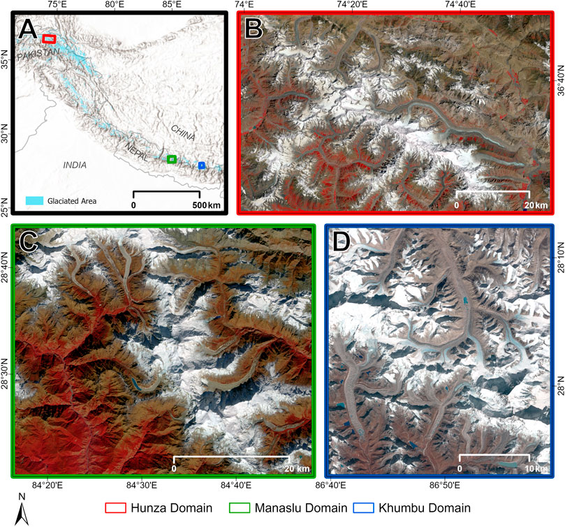
FIGURE 1. Overview of the study domains (A); Hunza, Karakoram (B); Manaslu, Central Himalayas (C); and the Khumbu, Central Himalayas (D). Background data for (A) is a world hillshade model accessed through ArcGIS Online. Sentinel-2 false colour composite (Near-infrared, Red, Blue) displayed in (B–D).

3.1 The Khumbu domain

The Khumbu domain (1,039 km²) is located in the Arun River and the Dudh Koshi basins to the north and south of the Nepal-China border, respectively. Glaciers in the southern part of this region are located at the northern limit of the summer monsoon, which provides 74% (∼359 mm) of the annual precipitation (∼485 mm a⁻¹) between June and September (Sherpa et al., 2017). Therefore, the glaciers on the southern side are summer-accumulation-type, simultaneously experiencing maximum accumulation and ablation during the summer (Benn and Owen, 2002; Thayyen and Gergan, 2010). Glaciers on the northern slope (on the Tibetan plateau) are located under a semi-arid, continental climate as the orographic divide reduces the influence of the summer monsoon (Yang et al., 2006). The Tingri weather station north of the orographic divide recorded a considerably lower annual average precipitation of 296.4 mm a⁻¹ (Yang et al., 2006). Sustained periods of negative mass balance budgets as a result of warming climates and weaker monsoons in the region (Bolch et al., 2011; Thakuri et al., 2014) have reduced glacier surface velocities, leading to the stagnation of debris-covered tongues and downwasting (Quincey et al., 2009; Rowan et al., 2021).

3.2 The Manaslu domain

The Manaslu domain (2,361 km²) is situated ∼230 km west of Mount Everest (Robson et al., 2018) in the Central Nepal Himalayas. Similarly to Khumbu, glaciers in this region are summer-accumulation-type. Climate data for the Manaslu region are limited, but the Larke Samdo weather station (3,650 m a.s.l.) recorded a mean annual precipitation of ∼1,000 mm a⁻¹ (Robson et al., 2018). Many of the lower parts of the debris-covered tongues in this region are stagnant (Robson et al., 2018; Racoviteanu et al., 2022a). The glaciers in the region are characterised by steep debris-covered tributaries that can be situated on slope gradients upwards of 30° and dense vegetation cover on their termini (Robson et al., 2015; Racoviteanu et al., 2022a).

3.3 The Hunza domain

The Hunza domain (4,033 km²) is located in the Gilgit-Baltistan territory of Pakistan. Glaciers in this region are winter-accumulation-type, with the westerly and south-westerly atmospheric circulations being the dominant sources of precipitation (Bookhagen and Burbank, 2010). The Batura Muztagh mountains impose orographic climatic controls over the region (Azam et al., 2018). Glaciers south of the divide are of maritime type, receiving mean annual precipitation of 1,500–1,800 mm a⁻¹. In contrast, glaciers north of the orographic divide are of continental type, receiving an estimated 600 mm a⁻¹ of mean annual precipitation (Winiger et al., 2005). Increased winter accumulation and cooler mean temperatures south of the orographic divide resulted in glacial mass gain between 1976 and 2012 in the region (Rankl et al., 2014). Glaciers in this region are highly dynamic (Hewitt, 2005; Rankl et al., 2014), exhibiting high surface velocities (Dehecq et al., 2019) and exhibiting stable, advancing, and surge-type behaviours, similar to the behaviours observed in the eastern regions of the Karakoram (Hewitt, 2005; Bolch et al., 2012; Brun et al., 2017).

4 Methodology

4.1 Datasets and pre-processing

4.1.1 Satellite imagery

The satellite imagery used in this study is listed in Table 1. Sentinel-2, launched in 2015, provides thirteen multispectral bands in the visible to shortwave infrared regions of the electromagnetic spectrum with spatial resolutions ranging from 10 to 60 m (Drusch et al., 2012). We used ten Sentinel-2 bands in the visible to the shortwave infrared region of the electromagnetic spectrum–blue, green, red, vegetation red edge, near-infrared (NIR), and shortwave infrared (SWIR)–for the years 2018 (Hunza domain) and 2019 (Manaslu and Khumbu domains) (Table 1). We panchromatically sharpened the imagery within PCI Geomatica CATALYST using a multi-resolution analysis fusion (González-Audícana et al., 2005). We used the Sentinel-2 bands to derive three indices: the Normalised Difference Vegetation Index (NDVI); the Normalised Difference Water Index (NDWI); and the Normalised Difference Snow Index (NDSI) (Figure 2).

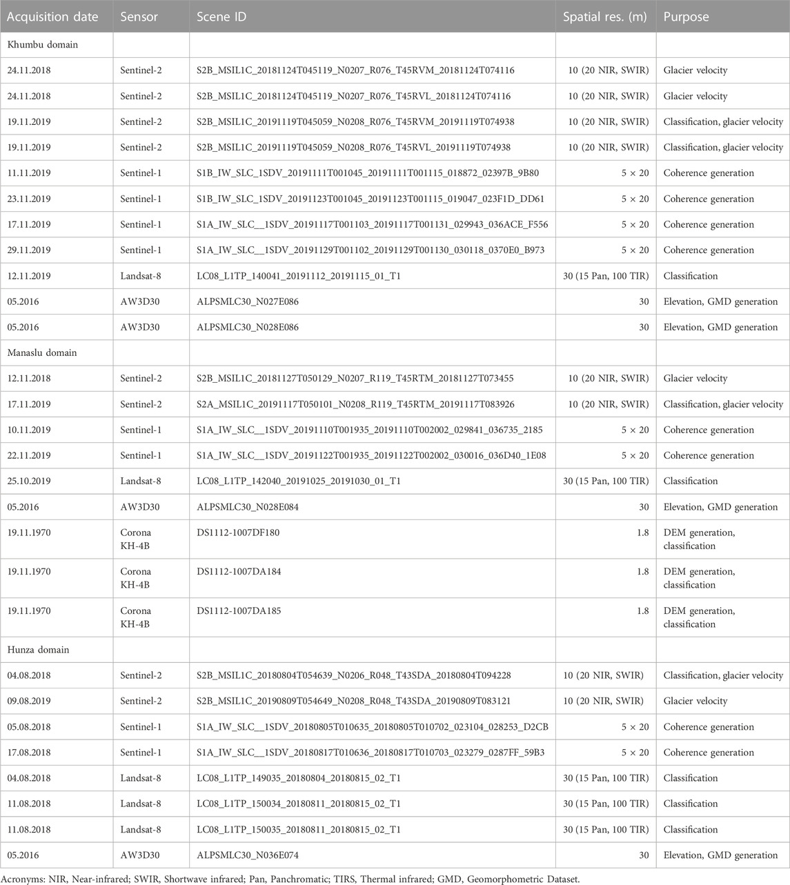
TABLE 1. Datasets used in this study.

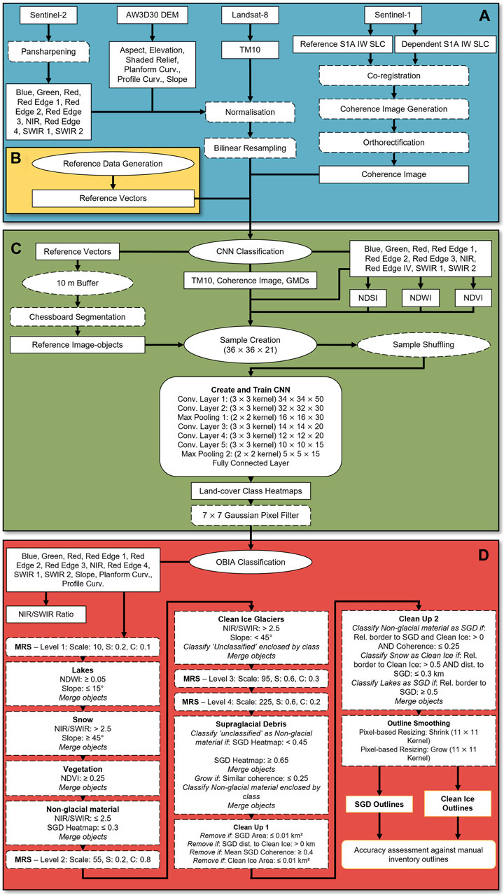
FIGURE 2. Flow chart outlining the methodology followed in this study. The method is divided into four sections: (A) dataset pre-processing; (B) reference vector dataset generation; (C) convolutional neural network classification; and (D) object-based image analysis refinement. Acronyms used: NIR, Near-infrared; SWIR, Shortwave infrared; Curv, Curvature; TM10, Thematic Mapper band 10; GMDs, Geomorphometric datasets; Conv, Convolutional; MRS, Multi-resolution segmentation; S, Shape; C, Compactness; NDWI, Normalised Difference Water Index; NDVI, Normalised Difference Vegetation Index; NDSI, Normalised Difference Snow Index; SGD, Supraglacial debris.

In addition, a second Sentinel-2 image acquired approximately 1 year apart (November 2018, August 2019) was used to derive a surface velocity dataset for each domain based on normalised cross-correlation (NCC) using the IMCORR Feature Tracking module within SAGA GIS 2.3.2. The surface velocity datasets were used in conjunction with Worldview-2 imagery accessed through ArcGIS Online to create the validation data for each study region.

We also obtained two Sentinel-1 single look complex (SLC) images in interferometric wide (IW) swath mode for the Hunza (2018), Khumbu and Manaslu (2019). Images were separated by a temporal baseline of 12 days and were co-registered using cross-correlation with the INSCOREG algorithm within PCI Geomatica CATALYST. The resulting image stack was used to generate a coherence raster which was converted to true ground range and orthorectified using the ALOS World 3D (AW3D30) DEM (Tadono et al., 2014) described in Section 4.1.2.

The Landsat-8 Thermal Infrared Sensor (TIRS), launched in 2013, provides two thermal infrared bands. We used the thermal infrared band TM10, with wavelengths of 10.60–11.19 µm (Roy et al., 2014) and a spatial resolution of 100 m, from approximately the same period as the Sentinel acquisitions (2018–2019).

All images described above were selected at the end of the ablation season (October-November in the Central Himalayas and July-August in the Karakoram) to ensure minimal cloud and transient snow cover.

4.1.2 Geomorphometric data

Elevation data used for the recent period was based on the AW3D30 DEM (30 m), produced using ALOS high-resolution stereo imagery acquired between 2006 and 2011, with an accuracy (root mean squared error, RMSE) of 6.84 m over High Mountain Asia (Liu et al., 2019). Although other DEMs were available, some of higher resolution, such as the HMA DEM (Shean, 2017), the AW3D30 has consistent coverage, with the lowest RMSE of the open access 30 m DEMs over High Mountain Asia and does not contain large data voids like the HMA DEM (Liu et al., 2019). We used the AW3D30 dataset to extract elevation and five geomorphometric datasets (slope angle, profile curvature, planform curvature, aspect, and shaded relief), which were subsequently used as layers in the classification procedure. The justification for each DEM derivative is given in Table 2.

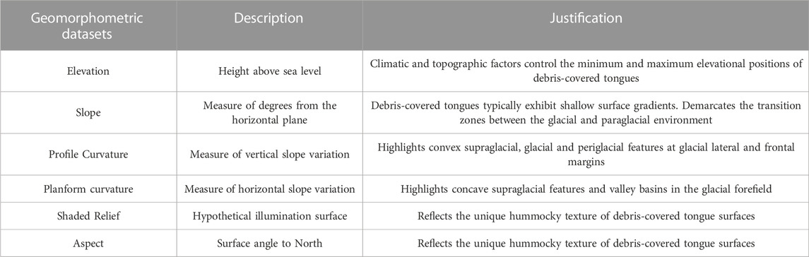
TABLE 2. Geomorphometric datasets used to train the CNN and justification for use.

All satellite and geomorphometric datasets were projected to UTM (zone 45 N for the Khumbu and Manaslu domains and UTM zone 43 N for the Hunza domain). For all datasets, pixel values were normalised between 0 and 1 and converted to 32-bit floating rasters using the SCALE algorithm within PCI Geomatica CATALYST. The Landsat-8, Sentinel-1 and AW3D30 datasets were bilinearly resampled to 10 m to match the spatial resolution of the Sentinel-2 imagery.

4.1.3 Corona datasets

To test our approach on panchromatic images from the 1970s, we used two Corona KH-4B images covering the Ponkar and Hinang sub-regions of the Manaslu domain. The Corona KH-4B satellite was developed as part of the US Keyhole (KH) space reconnaissance programme, which acquired ∼800,000 high-resolution (1.8–7.5 m) panchromatic images of Earth’s surface between 1960 and 1972 (Dashora et al., 2007). The Corona scenes were made available as fully processed orthomosaics at 2 m spatial resolution along with corresponding DEMs, extracted from these scenes using ERDAS Imagine, at 10 m spatial resolution (see Robson et al., 2018; Racoviteanu et al., 2022a). For details of the Corona imagery processing, the reader is directed to these papers. Elevation, slope angle, profile curvature, planform curvature, shaded relief and aspect geomorphometric datasets for the 1970s decade were generated from the 1970 Corona DEMs (10 m). The Corona imagery and geomorphometric datasets were normalised and converted to 32-bit floating rasters using the SCALE algorithm within PCI Geomatica CATALYST. The geomorphometric datasets were bilinearly resampled to 2 m to match the spatial resolution of the Corona images.

4.2 Reference vector data generation

For Sentinel and Corona imagery, we targeted the classification of seven predominant land-cover classes present in the imagery: supraglacial debris, clean ice, snow cover, lakes, vegetation, shadows, and non-glacial material. In order to train the CNN to recognise each of these classes, we generated a reference vector dataset for each class. The reference vector dataset was then used to automatically generate the training dataset. To avoid the laborious and time-consuming process of manually selecting sample locations to generate a high-quality training dataset, we used an automated reference vector data generation method adapted from Alifu et al. (2020) for application to multi-class output CNNs.

As a first step, we generated reference polygons for each land-cover class. For clean ice and supraglacial debris reference polygons, we relied on the freely available GAMDAM glacier inventory constructed based on Landsat ETM+ imagery and Google Earth imagery (Sakai, 2018). Since the polygons were provided over the entire glacier surface, we divided clean ice from supraglacial debris using a standard NIR/SWIR band ratio (Sentinel bands 7/9), with a threshold of 2.5. We randomly selected 30% of the debris cover polygons for reference vector generation using the random number generation routine in ArcGIS Pro 2.8.1 (n = 5 for Khumbu, n = 7 for Manaslu, n = 26 for Hunza). We used a slope threshold map of > 45° to separate snow from clean ice based on criteria used in other studies (e.g., Robson et al., 2015; Racoviteanu et al., 2021). For the lake polygons, we used the HMAv.1 lake dataset which was generated by thresholding the NDWI (Shugar et al., 2020). Vegetation polygons were generated using the NDVI derived from bands 4 and 8 with a threshold > 0.3. Shadow reference polygons were generated using the lowest 5% reflectance values in the blue Sentinel-2 multispectral band. The remainder of the unclassified area within the domain was assigned as non-glacial material.

Internal buffers were applied inside the reference polygons generated for each land-cover class so that the resulting reference vector points were not located near the boundary of land-cover classes. The buffer size (15–100 m) was selected according to the area coverage of the land-cover classes and the spectral similarity between neighbouring land-cover classes (Figure 3). Following this, we created reference vector points within the buffered reference polygons for each land-cover class to generate the reference vector dataset.

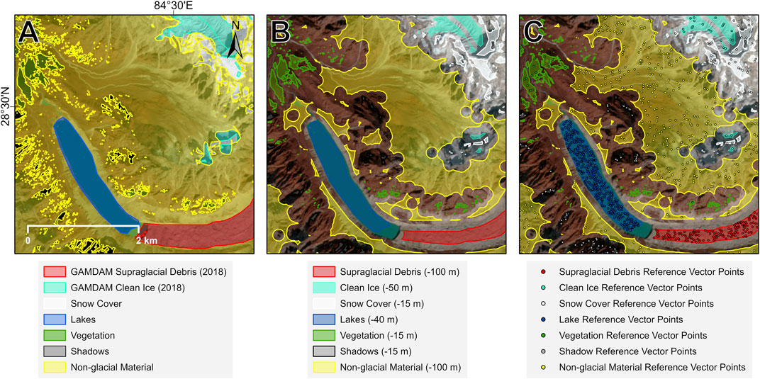
FIGURE 3. Automated generation of vector points illustration for CNN classification. (A) Outlines were created for each land-cover class in the study domains. (B) An internal buffer was applied to the outlines to reduce the influence of potentially problematic land-cover boundaries and increase training dataset quality. (C) Reference vector points were randomly generated within internal buffers.

Due to the difficulty of automating the generation of the 1970s reference vector dataset from panchromatic imagery, we manually adjusted the outlines based on the 2019 outlines in reference to the 1970 imagery to account for changes between 1970 and 2019. The resulting supraglacial debris polygons were split into training (40%) and validation (60%) data.

4.3 CNN inputs

We used all the available datasets as inputs for the CNN. The inputs consisted of ten Sentinel-2 bands (blue, green, red, vegetation red edge I-IV, NIR, SWIR I-II), Landsat-8 TM10, Sentinel-1 coherence, and six AW3D30 geomorphometric datasets. We used coherence to aid the identification of areas that have undergone glacier motion, deformation, or changing surface conditions. We employed TM10 to aid the differentiation between supraglacial and paraglacial debris based on land surface temperature differences. In addition, we included NDSI, NDWI and NDVI as inputs to help further differentiate between land-cover classes. The Corona classification used seven inputs: the panchromatic Corona image and the six geomorphometric datasets derived from the Corona DEM.

4.4 CNN-OBIA implementation

The CNN-OBIA approach was implemented in Trimble’s eCognition Developer 10.2 software using the open-source TensorFlow library, allowing for a seamless CNN and OBIA classification workflow.

4.4.1 Training datasets

To generate the training dataset from the reference vector dataset, as a first step, a 10 m buffer was created around each reference vector point created for each land-cover class presented in Section 4.2. The buffered vector points were then used to mark the locations for labelled training samples to be generated from for each land-cover class. We used land-cover prevalence and spectral signatures to determine the number of labelled training samples for each land-cover class, following Robson et al. (2020) (Table 3). The training dataset was composed of 69,500 samples (all classes cumulated) for each domain. For the Corona implementation, we also used a 10 × 10 m pixel buffer and generated 7,000 labelled training samples for each land-cover class, creating an accumulative training dataset of 49,000 samples.

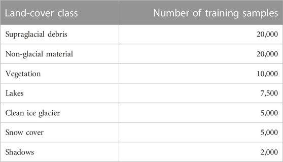
TABLE 3. The number of labelled training samples generated for each land-cover class.

4.4.2 CNN architecture

Following fine-tuning and cross-validation assessment (Supplementary Table S1; Supplementary Figures S1–S4 in the Supplement), a CNN with a five hidden layer architecture was selected (Figure 4). The best performing CNN had labelled training samples with dimensions of 36 × 36 × 21 and a hidden layer architecture of 3 × 3 × 50, 3 × 3 × 30, 3 × 3 × 20, 3 × 3 × 20, 3 × 3 × 15 with 3 × 3 convolutional kernels throughout and max pooling following the second and fifth layers. Max pooling employed 2 × 2 filters with a vertical and horizontal stride of 2. The classification was performed by a single fully connected layer with seven neurons. The minibatch size was set to 32, with a training step value of 5,000. The learning rate was set to 0.0001. The Corona imagery was classified using the same CNN architecture employed for the Sentinel-2 classification. The CNN trains in ∼5 min on a computer with 64 GB RAM, an Intel Core i7 processor, and an NVIDIA Quadro RTX 4000 graphics card.

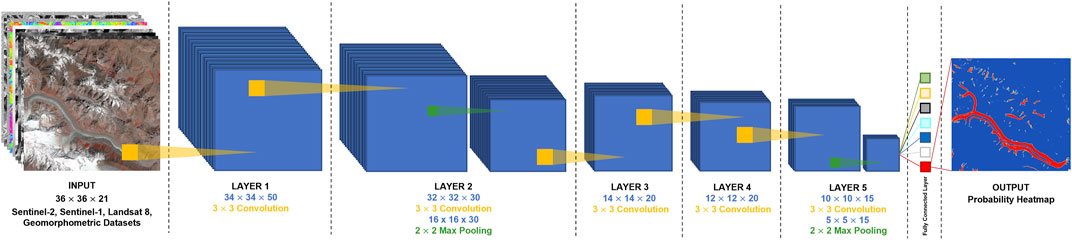
FIGURE 4. The CNN architecture employed in the current study. A five-layer CNN with a 36 × 36 × 21 input.

The CNN outputs a probability heatmap for each land-cover class in the training dataset. The outputted probability heatmaps were smoothed with a 7 × 7 Gaussian filter to reduce blurred boundary effects. We only employed the supraglacial debris heatmap for the subsequent debris-covered glacier OBIA classification, the other land-cover classes were classified according to fixed satellite datasets thresholds.

4.5 OBIA classification

In order to simplify the ruleset and ensure approach transferability among the three domains, we minimised the reliance of the OBIA ruleset on thresholds such as coherence, elevation and surface temperature that could differ between the supraglacial environments in the domains. Clean ice is mapped as a by-product of the OBIA supraglacial debris mapping procedure for both the Sentinel and Corona datasets. Although clean ice is not the focus of our paper, assessing the accuracy of the clean ice classification allows for our approach to be compared with previous approaches and for the overall inventory-creating potential of the approach to be assessed.

A four-level image segmentation was performed using the multi-resolution segmentation (MRS) algorithm (Table 4). MRS applies a mutual best-fitting approach to merge pixels into homogeneous image-objects (Baatz and Schape, 2000). MRS requires three parameters to be selected: scale, shape, and compactness. Segmentation quality heavily depends on the initial selection of these parameters (Rastner et al., 2014; Robson et al., 2015).

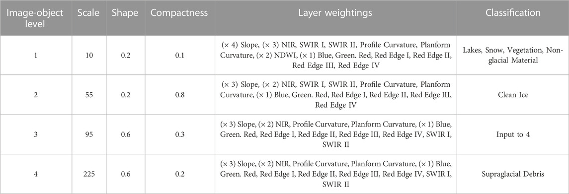
TABLE 4. Multi-resolution segmentation parameters for each image-object level.

Land-cover classes were classified according to fixed probability heatmap, spectral, geomorphometric, coherence and contextual thresholds (Figure 2). The resulting clean ice and supraglacial debris outlines were smoothed using pixel-based object resizing with an 11 $\times$ 11 surface tension window and a relative area threshold of < 50% for both growing and shrinking operations and were then exported as shapefiles.

The OBIA refinement for the Corona imagery was conducted in a similar manner as for the Sentinel data with the same segmentation scale parameter values as those used for the Sentinel classification. Shape and compactness were adjusted to account for the lack of pixel value variability. In the absence of multispectral bands, higher weightings were given to slope and curvature datasets. Land-cover classes were classified according to fixed probability heatmap, slope and contextual thresholds given in Table 5. Finally, image-objects were smoothed with pixel-based object resizing using 11 $\times$ 11 surface tension windows. Shrinking and growth occurred if supraglacial debris pixels occupied < 50% of the window.

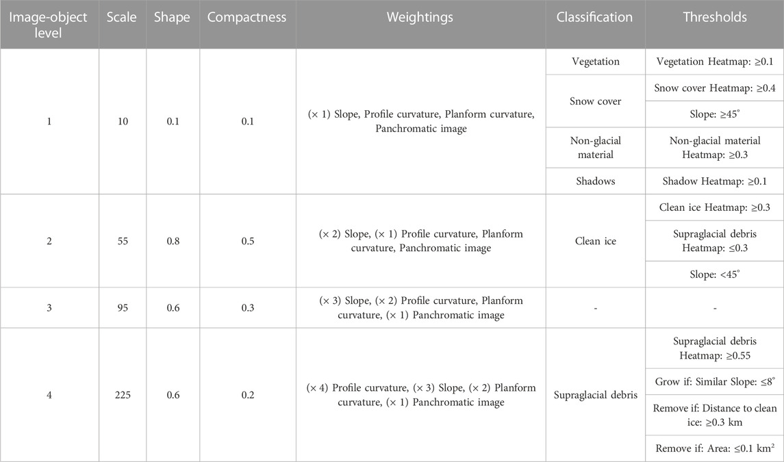
TABLE 5. Corona multi-resolution segmentation parameters and classification criteria for each image-object level.

4.6 Out-of-sample transfer learning methodology

As a separate experiment, we assessed the suitability of transfer learning on out-of-sample imagery. For this, we used the same network set-up as the one employed for the Sentinel-2 classification. We trained a CNN with training samples produced in one of the domains and transferred and applied it to the other two domains, iteratively. This process was performed for each domain. For example, the Khumbu CNN was trained using satellite and geomorphometric datasets from this domain, and the network was then transferred and applied to the satellite and geomorphometric datasets in the Hunza and Manaslu domains, which had not been used in the training dataset. Following the CNN classification, we performed the OBIA classification as described in Section 4.5.

4.7 Accuracy assessment

To assess the accuracy of the approach, we created a manually delineated glacier inventory derived from high-resolution 2016 Worldview-2 imagery, Sentinel-2 imagery, and Sentinel-1 coherence data. We only found minor changes in supraglacial debris extents between the Worldview-2 and the Sentinel-2 acquisition dates (2016-2019); these were insignificant at the 10 m resolution scale of the Sentinel-2 imagery. We used a surface velocity raster to separate the active ice from stagnant glacier tongues in the manual inventory. Ice flowing at velocities <2.5 m/a⁻¹ was assumed to be stagnant following Scherler et al. (2011) and Shukla and Garg (2020). We used the remaining 70% of the debris-covered glacier polygons that were not employed to generate the reference vector dataset to assess the accuracy of the approach. For the Corona classification, manually delineated debris-covered glacier outlines were made available from Racoviteanu et al. (2022a) to assess the accuracy of the approach.

Accuracy was assessed using three metrics: 1) a discrepancy estimation based on mapped glacier extent; 2) Intersection Over Union (IOU); and 3) a Precision-Recall plot. Discrepancy denotes the area deviation between automated and manually derived glacier outlines by measuring the percentage of over- and underestimation and has been used in previous studies to assess approach accuracy (e.g., Bolch et al., 2007; Bhambri et al., 2011; Bhardwaj et al., 2014; Alifu et al., 2020).

IOU measures the similarity between ground truth and the predicted occurrence of an object or entity in imagery and is a commonly used accuracy metric in computer vision object detection tasks. Detection is typically accepted as valid providing the IOU between the classification and ground truth bounding boxes exceeds a value of 0.7 (Jörgensen et al., 2019). The metric is calculated as (Eq. 1):

Precision-recall plots calculate the number of correctly and incorrectly assigned instances (Davis and Goadrich, 2006) for which there are four categories: 1) true positives (TP), the number of correctly identified positive instances; 2) false positives (FP), negative instances incorrectly assigned positive; 3) false negatives (FN), positive instances incorrectly assigned negative; and 4) true negatives (TN), the number of correctly identified negative instances.

True positive, false positive, and false negative instances were used to calculate Recall (R) and Precision (P). Recall measures the approach’s detection rate, determining how much of the actual debris-covered area was correctly identified (omission error). Precision measures the ability of the approach to identify non-debris-covered glacier area correctly (commission error) (Davis and Goadrich, 2006). Precision and Recall were used to calculate the F-score (F₁). F-score is a harmonic average of Recall and Precision and reports the accuracy of the approach (Goutte and Gaussier, 2005). The three measures were calculated from Eqs 2–4.

5 Results

5.1 Sentinel classification

5.1.1 OBIA clean ice classification

Clean ice was mapped with high accuracy in all domains, with F-scores exceeding 93% and IOU scores exceeding 89% when compared to the manual inventory (Table 6). Clean ice extent was underestimated by 3.2% in the Khumbu domain (177.8 out of 183.7 km²) and 2.3% in the Manaslu domain (136.6 of 139.7 km²) and was overestimated by 0.9% in the Hunza domain (583.1 out of 578.1 km²). Clean ice sections comprised 63.7% (Khumbu domain), 68.5% (Manaslu domain) and 69.9% (Hunza domain) of the total debris-covered glacier area and were situated on slopes with mean gradients of 17.1° in the Khumbu domain, 32.5° in the Manaslu domain, and 28.8° in the Hunza domain.

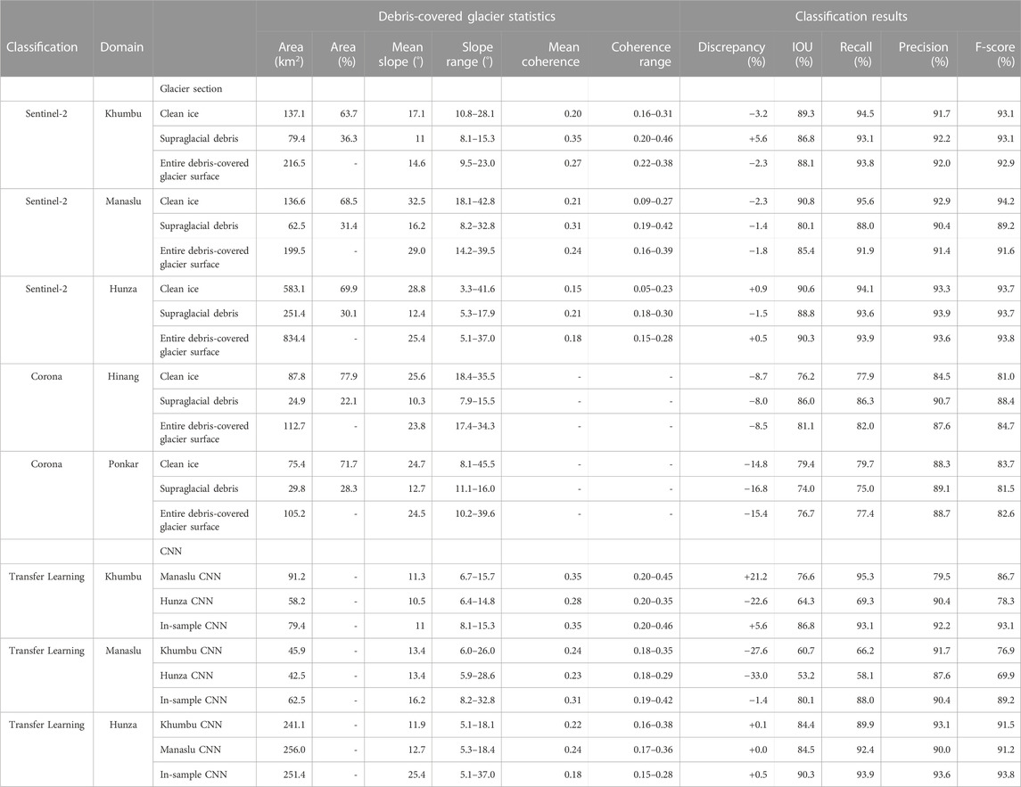
TABLE 6. Debris-covered glacier statistics and classification results from the Sentinel-2, Corona, and Transfer Learning classifications. Clean ice classification in Sentinel-2 image performed using OBIA only.

5.1.2 CNN-OBIA supraglacial debris classification

Using CNN-OBIA, we mapped 135 out of 160 debris-covered tongues featured in the manual glacier inventory across the three domains, with high accuracy, though slightly lower than clean ice sections (F₁ ≥ 89.2%) (Table 6). Supraglacial debris was overestimated by 5.6% in the Khumbu domain (79.4 out of 75.2 km²) (Figure 5), whereas it was underestimated by 1.4% in the Manaslu domain (62.5 out of 63.4 km²) (Figure 6) and 1.5% in the Hunza domain (251.4 out of 255.3 km²) (Figure 7). The IOU scores for each of the three domains (Khumbu 86.8%, Manaslu 80.1%, Hunza 88.8%) show a good agreement between CNN-OBIA and the validation data.

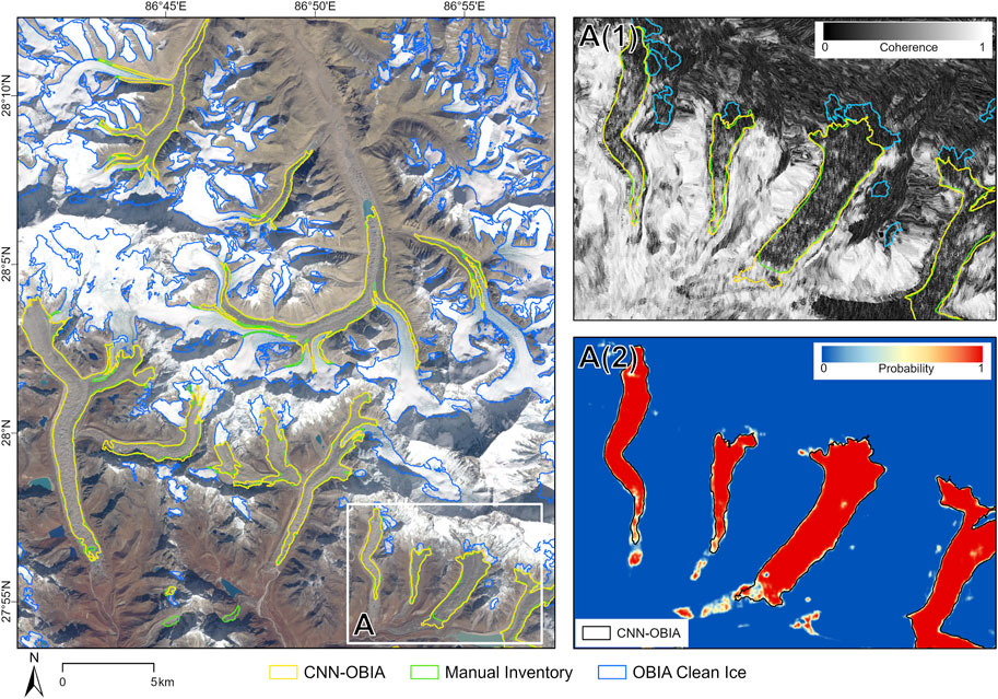
FIGURE 5. Comparison of automated CNN-OBIA outlines with the manual inventory in the Khumbu domain. A(1) In most cases, CNN-OBIA could detect the boundary between active and stagnant ice. A(2) The CNN was prone to misclassifying landforms with similar properties to supraglacial debris, such as the ice-cored moraine to the west of the Imja Tsho proglacial lake. Using OBIA thresholds, these types of misclassifications could be removed from the final glacier outlines. Sentinel-2 false colour composite (Near-infrared, Red, Blue) is displayed. Sentinel-1 coherence imagery displayed in A(1). CNN derived supraglacial debris probability heatmap displayed in A(2).

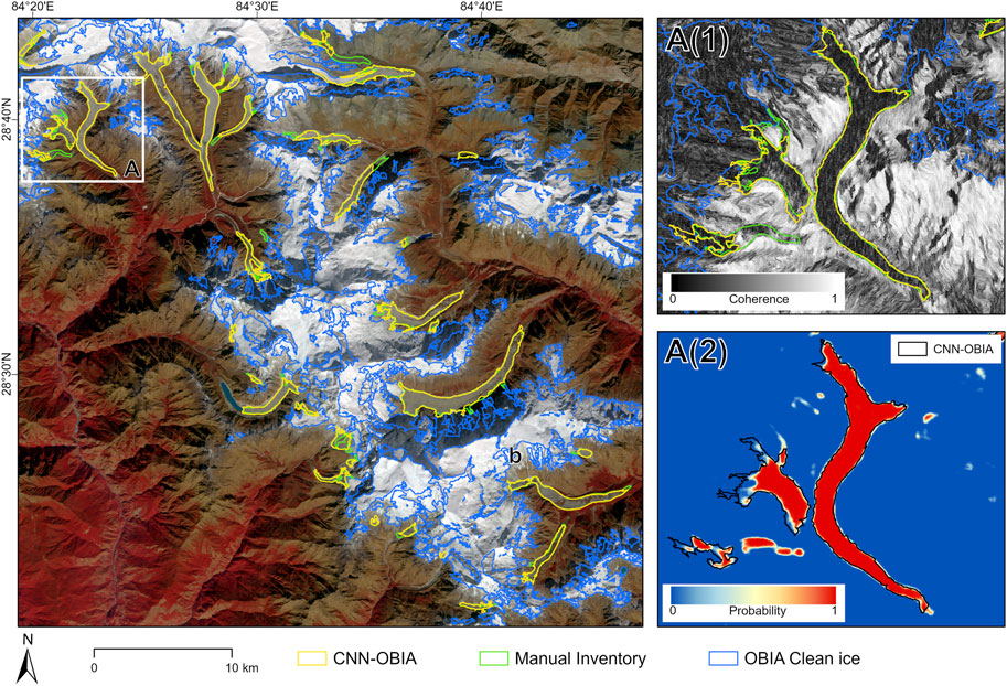
FIGURE 6. Comparison of CNN-OBIA outlines with the manual inventory in the Manaslu study region. Omission errors were common over steep, debris-covered tributary channels and steep slope gradient regions of the debris-covered glaciers (A1, A2). Sentinel-2 false colour composite (Near-infrared, Red, Blue) is displayed. Sentinel-1 coherence imagery displayed in A(1). CNN derived supraglacial debris probability heatmap displayed in A(2).

FIGURE 7. Comparison of CNN-OBIA outlines with the manual inventory in the Hunza study region. Notable discrepancies in area between the automated and manual inventory were caused by proglacial river channels such as those located at the terminus of the Kukuar glacier (A1, A2). Sentinel-2 false colour composite (Near-infrared, Red, Blue) is displayed. Sentinel-1 coherence imagery displayed in A(1). CNN derived supraglacial debris probability heatmap displayed in A(2).

Respective mean recall and precision accuracies of 91.6% and 92.2% indicate that commission and omission errors were relatively common; however, the difference between recall and precision accuracy scores varied between domains. The highest classification accuracy was achieved in the Hunza domain (F₁ = 93.7%), followed by the Khumbu domain (F₁ = 92.7%). CNN-OBIA achieved a lower accuracy for the supraglacial debris in the Manaslu domain (F₁ = 89.2%). Over the total debris-covered glacier surface area (i.e., clean ice and supraglacial debris combined), CNN-OBIA achieved accuracies up to 93.8%.

Glacier tongues featuring supraglacial debris had mean slope gradients of 11°, 12.4° and 16.2° in the Khumbu, Hunza, and Manaslu domains, respectively. However, the maximum slope gradients of debris-covered tongues in each domain varied greatly. For example, in the Khumbu and Hunza domains, supraglacial debris was situated on maximum slope gradients of 15.3° and 17.9°, compared to the supraglacial debris in the Manaslu domain that could be found on maximum slopes of 32.8°. This resulted in the steepest sections of the debris-covered area, which were primarily located at the clean ice-supraglacial debris transition zone, occasionally being omitted from the classification. Coherence also varied between the domains. The mean coherence observed in the Hunza domain (x̄ = 0.21) was significantly less than the mean coherence in both the Manaslu (x̄ = 0.31) and Khumbu (x̄ = 0.35) domains.

5.2 Corona classification

The extent of clean ice was underestimated in both images (Figure 8). Underestimation percentages ranged from 8.7% to 14.8%. In total, 87.8 out of 96.2 km² of clean ice was mapped in the Hinang area and 75.4 out of 88.5 km² in the Ponkar area of the Corona image. The IOU accuracies of 76.2% (Hinang) and 79.4% (Ponkar) indicate satisfactory agreement between CNN-OBIA outlines and the validation dataset. Clean ice was mapped in the two images with F-score accuracies of 81.0% in the Hinang area and 83.7% in the Ponkar area. Precision and recall accuracies indicate that omission errors were more common than commission errors. Clean ice sections had a mean slope gradient of 25.6° in the Hinang area and 24.7° in the Ponkar area image.

FIGURE 8. CNN-OBIA clean ice and supraglacial debris outlines delineated from Corona imagery over Ponkar (A1) and Hinang (B1). Corona panchromatic imagery displayed in A(1) and B(1). CNN derived supraglacial debris probability heatmap displayed in A(2) and B(2). CNN derived clean ice probability heatmap displayed in A(3) and B(3).

CNN-OBIA identified 14 of 18 debris-covered tongues featured in the validation data across the two Corona images. Supraglacial debris extent was underestimated by 8.0% in the Hinang area (24.9 out of 27.1 km²) and by 16.8% in the Ponkar image (29.8 out of 35.8 km²). The measured IOU accuracy scores were 86.0% (Hinang) and 74.0% (Ponkar), indicating satisfactory network performance (Table 6).

The overall performance of CNN-OBIA to classify supraglacial debris was high, with reported F-scores in the Hinang and Ponkar areas of 88.4% and 81.5%, respectively. The precision and recall scores indicate that omission errors were more common than commission errors. CNN-OBIA achieved F-score accuracies of 84.7% (Hinang) and 82.6% (Ponkar) over the entire debris-covered glacier surface area (clean ice and supraglacial debris). Debris-covered tongues had mean slope gradients of 10.3° and 12.7° in the Hinang and Ponkar images, respectively.

5.3 Out-of-sample transfer learning for debris-covered glacier delineation

The results of the transfer learning approach are presented in Table 6 and highlight that transfer learning was more successful in some directions than others. Transfer learning proved challenging to apply in the Khumbu and Manaslu domains, producing F-scores between 69.9% and 86.7% and IOU scores between 53.2% and 76.6%. Conversely, transferred networks could classify out-of-sample Hunza imagery with F-score accuracies comparable to the network trained using in-sample imagery in the Hunza domain (91.2% and 91.5% versus 93.7%). The results of the transfer learning experiment show that omission errors are far more common than commission errors when classifying out-of-sample imagery.

In the Khumbu domain, supraglacial debris extent was overestimated by 21.2% by the Manaslu CNN (91.2 out of 75.2 km²) but underestimated by 22.6% (58.2 out of 75.2 km²) by the Hunza CNN. Debris-covered tongues mapped by the transfer CNNs had mean slope gradients of 11.3° (Manaslu CNN) and 10.5° (Hunza CNN) and mean coherence values of 0.35 and 0.28. The highest mean coherence value of a debris-covered tongue mapped by the Hunza CNN was 0.32, whereas the highest mapped by the Manaslu CNN was 0.45.

In the Manaslu domain, supraglacial debris extent was underestimated by both the Khumbu and Hunza CNNs by 27.6% (45.9 out of 63.4 km²) and 33.0% (42.5 out of 63.4 km²), respectively. Debris-covered tongues mapped by the Khumbu CNN had a mean slope gradient of 13.4° and mean coherence values of 0.24. Similarly, those mapped by the Hunza CNN had a mean slope gradient of 13.4° and a mean coherence value of 0.23. The note-worthy difference between the debris-covered tongues mapped by the Khumbu CNN and Hunza CNN is the maximum coherence value mapped by both CNNs; 0.35 and 0.27, respectively.

In the Hunza domain, supraglacial debris extent was overestimated by 5.6% by the Khumbu CNN (241.1 out of 255.3 km²) and by 0.3% by the Manaslu CNN (256.0 out of 255.3 km²). The mean slope gradient and mean coherence value of the debris-covered tongues mapped by the Khumbu CNN were 11.9° and 0.22, respectively. In comparison, the mean slope gradient and coherence values of those mapped by the Manaslu CNN were 12.7° and 0.24, respectively.

6 Discussion

6.1 Integration of CNNs and OBIA to classify debris-covered glaciers

The CNN-OBIA classification approach developed in the current study demonstrates high-accuracy performances in three distinct domains. CNN-OBIA produced F-scores up to 93.7% for supraglacial debris across the three domains, indicating that the combination of deep learning and OBIA is a robust and accurate tool for delineating the extent of supraglacial debris cover in complex glacial environments. CNN-OBIA operates with minimal analyst input, has the ability to generate debris-covered glacier outlines relatively quickly (∼13 min), and is equally applicable across our three study areas with varying climates, topographies and supraglacial environments. Additionally, employing OBIA to map clean ice in the same workflow as debris-covered glaciers illustrates the capacity of the CNN-OBIA approach to create complete glacier inventories with high accuracies (F₁ = 93.8%).

Integrating CNN and OBIA into one classification approach addresses some of the shortcomings of CNN classifications. For example, spatial downsampling provides CNNs with a powerful generalisation ability, which allows CNNs to perform well when classifying land-cover classes with large amounts of intra-class variation such as supraglacial debris cover. However, downsampling results in the loss of the specific arrangement of features (Zhao et al., 2017), making it difficult for CNNs to predict the exact boundary between land-cover classes (Jin et al., 2019). This results in blurred land-cover borders, for example, between the debris-covered glacier and the lateral moraines. This would have resulted in an 11% overestimation of the total debris-covered area in the Khumbu domain if the CNN output was the sole basis for the classification. Utilising OBIA to refine the CNN output allows the glacier boundary positions to be repositioned inside the glacial margin, significantly improving the accuracy of the approach.

Furthermore, CNNs are prone to misclassifying land-cover classes due to label noise or the sharing of similar properties to supraglacial debris. Employing OBIA thresholding allows these misclassifications to be removed through masking or utilising contextual information in the classification. Since OBIA is capable of classifying land-cover classes based on empirically thresholding low-level features, commonly commissioned land-cover classes such as waterbodies and vegetation can be masked out from further analysis, preventing the inclusion of CNN misclassifications in the final delineated debris-covered glacier area. This function may be especially advantageous when working with multi-class output CNNs, label noise in the training dataset, or unbalanced training datasets (Fernández et al., 2018).

Employing OBIA contextual-based rules such as distance from clean ice, combined with shape rules such as minimum area coverage also allows misclassifications caused by the similarity between landforms, such as mass movement deposits and ice-cored moraines, to be rectified (Figure 5). However, it should be noted that if the misclassified area features high probability values and extends out from the supraglacial debris area delineated by the CNN (see Section 6.2; Figure 7), it is not possible to omit these commission errors without additional, potentially excessive OBIA thresholds. These additional thresholds would likely significantly reduce the transferability of an integrated CNN and OBIA approach between regions.

To further demonstrate the benefit of integrating two classification methods into one seamless classification approach, we produced a precision-recall plot on supraglacial debris outlines in the Khumbu domain delineated without OBIA, where the probability heatmap threshold was ≥ 0.65. The PRC plot showed that recall accuracy increased by 0.9% and precision accuracy increased by 4.2% when OBIA was conducted following CNN classification, resulting in an F-score accuracy of 2.6%. As indicated by this increase in F-score accuracy, employing OBIA following a CNN classification allows debris-covered glacier extents to be mapped with higher accuracy than those delineated solely relying on the CNN classification. Therefore, OBIA could prove to be a beneficial addition to CNN image classification workflows for all other glacial, and indeed, non-glacial land-cover mapping tasks.

6.2 Sentinel-2 classification commission and omission errors

Commission errors appear as extensions of glacier outlines beyond the glacial margin into the landforms in the adjacent terrain, rather than misclassified landforms away from the glacial margins. For example, while in most cases, CNN-OBIA was capable of mapping the boundary between active and stagnant ice, the extension of CNN-OBIA outlines into stagnant ice occurred where the stagnant side of the active-stagnant boundary presented supraglacial lakes (Figure 5A2). Commission errors were also commonly caused by the presence of proglacial river channels in both narrow, steep channels and expansive, shallow gradient glacial forefields (Figure 7A1). Additionally, CNN-OBIA was prone to including shallow slope gradient lateral moraines in the demarcated glacier area, such as those in the Manaslu domain. These commission errors can likely be attributed to the sharing of similar coherence, geomorphometric, and spectral properties to supraglacial debris. This would reduce the amount of inter-class variation, potentially creating class overlap in feature space. Class overlap confounds the CNN’s ability to differentiate between the debris-covered tongue and the adjacent landforms with similar properties, resulting in their inclusion in the glacier outlines.

On the other hand, omission errors were cases of missing entire glaciers that were in the manual inventory. Upon visual analysis, these small glaciers were typically < 0.5 km² in size or located on steep slopes with gradients > 24°. Steep gradient debris-covered glacier termini and topography in the domains were sources of omission errors; for example, CNN-OBIA underestimated the position of debris-covered glacier termini with slope gradients > 24° in the Hunza domain and steep debris-covered tributaries in the Manaslu domain (Figure 6A1). The CNN could not classify these debris-covered regions due to a lack of intra-class variation within the supraglacial debris samples. These regions were likely not included in the labelled training samples because the reference dataset creation method prevents labelled samples from being extracted from areas near potentially problematic land-cover boundaries. Thus, the CNN was not trained to recognise supraglacial debris on steep slopes and termini as part of debris-covered tongues, leading to their exclusion from the glacier outlines. Omission errors were also caused by shadows on the margins of debris-covered tongue surfaces; however, this omission accounted for only 0.15% of the total debris-covered area across the three study regions (0.61 out of 393.9 km²).

6.3 Classifying debris-covered glaciers in historical imagery

We successfully adapted and applied our CNN to declassified Corona imagery, yielding F-score accuracies up to 87.4% for the supraglacial debris though this is still subject to further improvements.

Supraglacial debris coverage was underestimated in both Corona images (Figure 8), with misclassifications typically occurring between the glacier boundaries and the lateral moraines. In addition, outlines occasionally extended into the adjacent paraglacial material, especially if the paraglacial material exhibited similar geomorphometric properties to the debris-covered surface. Furthermore, debris-covered glaciers exhibiting low panchromatic band values across their entire surface were omitted by the CNN-OBIA classification. However, CNN-OBIA outlines were not sensitive to supraglacial debris lithology changes on the debris-covered tongue surfaces in the Hinang and Ponkar areas, which produce alternating sections of high and low panchromatic values.

In the absence of multispectral data, the Corona-based classification relied heavily on the panchromatic band, causing paraglacial landforms that exhibit high panchromatic values and geomorphometric properties similar to supraglacial debris or clean ice, such as river channels, frozen lakes, and debris flows, to be frequent sources of commission error. Clean ice and supraglacial debris were also frequently misclassified as one another. Furthermore, we found that the surface of the debris-covered tongues reflected in the high-resolution geomorphometric datasets shared similar textures with the lateral moraines, leading to the inclusion of lateral moraines in the delineated supraglacial debris extent and adding an average of 8.5% to the total delineated debris-covered area across the two Corona images. These misclassification examples can likely be explained by class overlap in feature space as there are fewer CNN inputs to provide the necessary discriminatory high-level features.

The smaller number of inputs for the Corona classification may have also caused a degree of network overfitting (Webb, 2011; Cogswell et al., 2016; Baduma and Locascio, 2017). The CNN employed to classify the Corona imagery had the same architecture used in the Sentinel-2 classification. The removal of inputs can significantly affect network performance. The Corona classification was performed with seven inputs instead of the twenty-one inputs it was optimised for; therefore, the CNN architecture may have been too complex for the mapping task, leading to overfitting and subsequent misclassifications. The performance of a CNN fine-tuned to handle the smaller number of input data would most likely exceed the performance of the CNN architecture employed in this study.

6.4 Influence of out-of-sample training data on CNN performance

In terms of misclassification, transfer learning CNNs failed to map lithological changes on the debris-covered tongues caused by rockfall deposits (Figure 9). The Hunza CNN was also incapable of mapping large regions in the lower reaches of the debris-covered tongues with high coherence values in the Khumbu and Manaslu regions. Debris-covered tongues in all three domains situated on slopes with gradients > 22° were frequently omitted from the transfer learning outlines. Shaded regions of the glaciers were also omitted. Commission errors were less common, as indicated by the high precision accuracies. However, the Manaslu CNN outlines frequently extended beyond the glacial margin onto lateral moraines and into the paraglacial environment, resulting in the lowest precision accuracies among the three CNNs. The commission of lateral moraines was the primary reason for the low precision accuracy in the Khumbu region, resulting in an additional 17.3% (15.4 km²) of supraglacial debris area coverage.

FIGURE 9. A visual comparison of Sentinel-2 multispectral imagery (A) and the CNN supraglacial debris probability heatmap (B) produced by the Hunza CNN over the Kechakyu glacier, Manaslu. Note how the location of low probability values in the heatmap corresponds to the location of lithological changes on the debris-covered surface in the Sentinel-2 image. The relationship between probability heatmap values and reflectance in Sentinel-2 near-infrared band is shown in (C). Sentinel-2 false colour composite (Near-infrared, Red, Blue) is displayed in (A). CNN derived supraglacial debris probability heatmap displayed in (B).

The results of the transfer learning experiment illustrate that transfer learning applied to out-of-sample imagery was not as successful as CNNs trained on in-sample imagery in their respective regions. These results indicate that high-level features derived from a training dataset in one training region may not fully represent the debris-covered surface properties in another region. Therefore, training data from the region to be mapped is an essential prerequisite on regional scales. This reflects that the surfaces of debris-covered tongues are influenced by varying climate forcing, dynamics, topographies, lithologies and surface processes resulting in spatial variation across High Mountain Asia.

For example, debris-covered tongues in the Hunza domain exhibit low coherence values across their surfaces (x̄ = 0.21), whereas those in the Khumbu domain exhibit substantially higher values (x̄ = 0.35), which could partially relate to greater surface velocities and more active glacier flow in the Hunza domain (Dehecq et al., 2019). Therefore, the distribution of the Hunza training samples across feature space was insufficient for the Hunza CNN to fit the coherence properties it had learnt to the Khumbu domain. This is evident in the probability heatmap outputted by the Hunza CNN, where low probability values are correlated with debris-covered regions with high coherence values.

Another example of the correlation between low probability heatmap values and region-specific surface characteristics is the rockfall deposits on the surfaces of the debris-covered tongues in the Manaslu region (Figure 9). The rockfall deposits have a different spectral signature to the debris transported by other processes to the surface, reflecting less light in each multispectral band. Since these rockfall deposits are not present in the Hunza and Khumbu domains, their respective CNNs were not trained with the sample heterogeneity required to recognise rockfall deposits as features of the debris-covered environment causing rockfall deposits to not be mapped by the transfer CNNs.

However, transfer learning worked better when applied to the Hunza domain using a CNNs trained in the Khumbu and Manaslu domains. This highlights the importance of intra-class variation in training datasets and suggests it is beneficial to generate samples in regions with diverse debris-covered surface characteristics, or to accumulate training samples from multiple regions, to provide the intra-class variance required to avoid significant omission errors in out-of-sample imagery.

The results of the transfer learning experiment highlight the complexity of applying out-of-sample transfer learning approaches to create large-scale glacier inventories across High Mountain Asia. Future studies should continue to test the applicability of out-of-sample transfer learning for debris-covered glacier mapping since the method holds the potential to significantly reduce the amount of time required to produce accurate glacier outlines in data-scarce regions.

6.5 Comparison with previous debris-covered glacier methods

Our CNN-OBIA approach achieved F-score accuracies between 89.2% and 93.7% in three separate regions ranging from 1,039 km² to 4,033 km² in size. Thus, the domains are considerably larger than those used in the majority of previous debris-covered glacier mapping studies. Our CNN-OBIA approach also produced outlines with similar accuracies compared to those achieved over single glaciers (e.g., Karimi et al., 2012; Shukla and Ali, 2016; Lippl et al., 2018), indicating that our CNN-OBIA approach is a highly robust and accurate, and capable of operating over large, glaciated regions.

One of the major strengths of our CNN-OBIA approach compared to other methods is that, unlike other methods, it does not rely on fixed thresholds that vary from glacier to glacier or region to region to classify supraglacial debris, for example, slope gradient (e.g., Paul et al., 2004; Ghosh et al., 2014; Lippl et al., 2018), surface temperature (e.g., Bhambri et al., 2011; Rastner et al., 2014; Robson et al., 2016), and band ratio values (e.g., Racoviteanu and Williams, 2012; Alifu et al., 2015; Shukla and Ali, 2016). The minimal reliance of CNN-OBIA on fixed thresholds allows it to be applied across multiple regions without modifications and makes it superior to many existing approaches for mapping supraglacial debris cover.

The CNN employed in our approach has a relatively simple structure, i.e., it does not include features such as encoding and decoding stages (e.g., Xie et al., 2020; Xie et al., 2021) or attention mechanisms (e.g., Tian et al., 2022) within its architecture. Therefore, this simple CNN structure might not be fully suited to the complexities of large-scale glacier mapping applications. Networks such as DeepLabV3+ have proven to be very capable of handling these complexities (Xie et al., 2021); however, integrating OBIA following CNN classification allowed our approach to perform similarly to the DeepLabV3+ network utilised by Xie et al. (2021), with high F-score accuracies (93.7%, 92.7, 89.2% versus 92.6%) in complex high-mountain glacial environments despite the simplicity of our CNN structure. OBIA was particularly useful for removing misclassifications related to lakes and similar landforms that previous studies struggled with (Xie et al., 2020; Tian et al., 2022).

However, CNN-OBIA was prone to common debris-covered glacier mapping pitfalls experienced by previous approaches, such as omitting steep (≥25°) glacial tributaries (e.g., Robson et al., 2015) from the delineated debris-covered area. Previously mentioned proglacial river channels were also frequently commissioned, similarly to previous approaches (e.g., Robson et al., 2015; Alifu et al., 2020; Xie et al., 2020). However, CNN-OBIA allowed the mapping of debris-covered tongues with distinct lithological changes, often mapped as separate entities (e.g., Robson et al., 2015) to be classified as single glacier units, such as the Himal Chuli and Kechakya glaciers in the Manaslu region. This is an improvement compared to previous approaches.

7 Summary and further work

We developed a simple, transferable CNN–OBIA approach that was able to classify supraglacial debris with F-score accuracies up to 93.7% across the three domains based on freely available multispectral, geomorphometric, thermal, and coherence datasets. Despite encountering common debris-covered glacier mapping omission errors mentioned above, the integration of OBIA following CNN classification into one seamless approach allowed most errors to be rectified during the primary classification process, reducing the amount of analyst input required to improve classification accuracies.

CNN-OBIA also showed promise for mapping debris-covered glaciers in historical Corona satellite imagery, producing F-score accuracies up to 84.7% over the entire debris-covered glacier surface. We believe the approach holds the potential to streamline the creation of historical glacier inventories across the wider HMA region. To the best of the authors’ knowledge, our study is the first to automatically map debris-covered glaciers in Corona imagery and to further test its ability for multitemporal inventory creation. The approach also holds the potential to automate the detection of other geomorphological entities such as landslides, lava flows, permafrost, and quaternary landforms in historical panchromatic imagery. However, due to the limited area covered by the Corona data, further work is needed to assess the suitability of the approach to classify debris-covered glaciers in historical datasets. We suggest that the inclusion of other Corona-derived datasets, such as texture, will help improve the ability of the CNN to distinguish different landforms from panchromatic imagery, and this can be explored in a subsequent study.

With respect to transfer learning applied to out-of-sample imagery, we found that it was heavily dependent on the distribution of debris-covered surface characteristics across sample space and the amount of intra-class variation present in the training dataset. Our experiments showed that the extreme variations of high mountain glacial environments and debris-covered glacier surface characteristics pose significant challenges for the application of transfer learning to out-of-sample imagery for streamlining regional glacier inventory creation. Further work is needed to improve the application of out-of-sample transfer learning to debris-covered glacier mapping. This includes generating extensive training datasets with samples gathered from diverse geographical regions, which capture the complexities of debris-covered tongue surface characteristics. This also illustrates the necessity for future studies to continue to establish the optimal network architecture and parameters, training dataset qualities, and a consensus on the best remote sensing datasets to employ for mapping.

Furthermore, to greatly enhance our ability to produce highly accurate debris-covered and clean ice glacier outlines over large spatial scales, we suggest the addition of OBIA following the classification of more complex network architectures, such as DeepLabV3+. These integrated CNN and OBIA classification approaches can be used for more complex land-cover classification tasks in both contemporary and historical satellite imagery, not just for debris-covered glacier mapping.

Lastly, based on the ability of the network used in this study to distinguish between active and stagnant ice, we suggest the inclusion of interferometric coherence imagery as an input to all future networks to address the limitations encountered by previous deep learning methods (e.g., Lu et al., 2021).

Data availability statement

Publicly available datasets were analyzed in this study. This data can be found here: AW3D30 was obtained from the JAXA Earth Observation Research Center (EORC) (http://www.eorc.jaxa.jp/ALOS/en/aw3d30/index.htm). Landsat and Sentinel-2 imagery was obtained from USGS Global Visualisation Viewer (GloVis) (https://glovis.usgs.gov/). Sentinel-1 imagery was obtained from the ASF Data Search Vertex (https://search.asf.alaska.edu/). The GAMDAM glacier inventory is available from PANGAEA (https://doi.pangaea.de/10.1594/PANGAEA.891423). The Himalayan glacial lake inventory is available from NSIDC (https://nsidc.org/data/hma_gli/versions/1). Worldview-2 imagery was accessed through ArcGIS Online (https://services.arcgisonline.com/ArcGIS/rest/services/World_Imagery/MapServer).

Author contributions

DT, BR, and AR contributed to the conceptualisation of the study. DT and BR designed the study. DT and BR processed the datasets. DT performed the analysis. DT wrote the first draft of the manuscript. DT and AR wrote sections of the manuscript. All authors contributed to the article and approved the submitted version.

Acknowledgments

We acknowledge the Japan Aerospace Exploration Agency (JAXA) for providing the AW3D30 data, the USGS/NASA for providing Landsat data, and the ESA for providing Sentinel-1 and Sentinel- 2 data.

Conflict of interest

The authors declare that the research was conducted in the absence of any commercial or financial relationships that could be construed as a potential conflict of interest.

Publisher’s note

All claims expressed in this article are solely those of the authors and do not necessarily represent those of their affiliated organizations, or those of the publisher, the editors and the reviewers. Any product that may be evaluated in this article, or claim that may be made by its manufacturer, is not guaranteed or endorsed by the publisher.

Supplementary material

The Supplementary Material for this article can be found online at: https://www.frontiersin.org/articles/10.3389/frsen.2023.1161530/full#supplementary-material

References

Alifu, H., Tateishi, R., and Johnson, B. (2015). A new band ratio technique for mapping debris-covered glaciers using Landsat imagery and a digital elevation model. Int. J. Remote Sens. 36, 2063–2075. doi:10.1080/2150704x.2015.1034886
Alifu, H., Vuillaume, J. F., Johnson, B. A., and Hirabayashi, Y. (2020). Machine-learning classification of debris-covered glaciers using a combination of Sentinel-1/-2 (SAR/optical), Landsat 8 (thermal) and digital elevation data. Geomorphology 369, 107365. doi:10.1016/j.geomorph.2020.107365
Anderson, L. S., and Anderson, R. S. (2016). Modeling debris-covered glaciers: Response to steady debris deposition. Cryosphere 10, 1105–1124. doi:10.5194/tc-10-1105-2016
Azam, M. F., Wagnon, P., Berthier, E., Vincent, C., Fujita, K., and Kargel, J. S. (2018). Review of the status and mass changes of Himalayan-Karakoram glaciers. J. Glaciol. 64, 61–74. doi:10.1017/jog.2017.86
Baatz, M., and Schape, A. (2000). “Multiresolution Segmentation: An optimisation approach for high quality multi-scale image segmentation,” in Beutrage zum AGIT-Symposium (Wichmann Verlag, Karlsruhe, Germany: Spinger).
Baduma, N., and Locascio, N. (2017). Fundamentals of deep learning: Designing next-generation machine intelligence algorithms. Sebastopol, CA: O'Reilly Media, Inc.
Baumhoer, C. A., Dietz, A. J., Kneisel, C., and Kuenzer, C. (2019). Automated extraction of Antarctic glacier and ice shelf fronts from Sentinel-1 imagery using deep learning. Remote Sens. 11 (21), 2529. doi:10.3390/rs11212529
Benn, D. I., and Owen, L. A. (2002). Himalayan glacial sedimentary environments: A framework for reconstructing and dating the former extent of glaciers in high mountains. Quat. Int. 97-98, 3–25. doi:10.1016/S1040-6182(02)00048-4
Benz, U. C., Hofmann, P., Willhauck, G., Lingenfelder, I., and Heynen, M. (2004). Multi-resolution, object-oriented fuzzy analysis of remote sensing data for GIS-ready information. ISPRS J. Photogrammetry Remote Sens. 58, 239–258. doi:10.1016/j.isprsjprs.2003.10.002
Bhambri, R., Bolch, T., and Chaujar, R. K. (2011). Mapping of debris-covered glaciers in the Garhwal Himalayas using ASTER DEMs and thermal data. Int. J. Remote Sens. 32, 8095–8119. doi:10.1080/01431161.2010.532821
Bhardwaj, A., Joshi, P. K., SnehmaniSingh, M. K., Sam, L., and Gupta, R. D. (2014). Mapping debris-covered glaciers and identifying factors affecting the accuracy. Cold Regions Sci. Technol. 106-107, 161–174. doi:10.1016/j.coldregions.2014.07.006
Bianchi, F. M., Grahn, J., Eckerstorfer, M., Malnes, E., and Vickers, H. (2021). Snow avalanche segmentation in SAR images with fully convolutional neural networks. IEEE J. Sel. Top. Appl. Earth Observations Remote Sens. 14, 75–82. doi:10.1109/JSTARS.2020.3036914
Blaschke, T., Hay, G. J., Kelly, M., Lang, S., Hofmann, P., Addink, E., et al. (2014). Geographic object-based image analysis - towards a new paradigm. ISPRS J. Photogrammetry Remote Sens. 87, 180–191. doi:10.1016/j.isprsjprs.2013.09.014
Bolch, T., Buchroithner, M. F., Kunert, A., and Kamp, U. (2007). “Automated delineation of debris-covered glaciers based on ASTER data,” in GeoInformation in europe. Editor M. A. Gomarasca (Netherlands: Milpress).
Bolch, T., Kulkarni, A., Kääb, A., Huggel, C., Paul, F., Cogley, J. G., et al. (2012). The state and fate of Himalayan glaciers. Science 336, 310–314. doi:10.1126/science.1215828
Bolch, T., Pieczonka, T., and Benn, D. I. (2011). Multi-decadal mass loss of glaciers in the Everest area (Nepal Himalaya) derived from stereo imagery. Cryosphere 5, 349–358. doi:10.5194/tc-5-349-2011
Bookhagen, B., and Burbank, D. W. (2010). Toward a complete Himalayan hydrological budget: Spatiotemporal distribution of snowmelt and rainfall and their impact on river discharge. J. Geophys. Res. 115, 03019. doi:10.1029/2009jf001426
Brun, F., Berthier, E., Wagnon, P., Kaab, A., and Treichler, D. (2017). A spatially resolved estimate of High Mountain Asia glacier mass balances from 2000 to 2016. Nat. Geosci. 10, 668–673. doi:10.1038/NGEO2999
Burns, P., and Nolin, A. (2014). Using atmospherically-corrected Landsat imagery to measure glacier area change in the Cordillera Blanca, Peru from 1987 to 2010. Remote Sens. Environ. 140, 165–178. doi:10.1016/j.rse.2013.08.026
Cogswell, M., Ahmed, F., Girshick, R. B., Zitnick, C. L., and Batra, D. (2016). Reducing overfitting in deep networks by decorrelating representations. Comput. Res. Repos. 1511, 06068. doi:10.48550/arXiv.1511.06068
Dashora, A., Lohani, B., and Malik, J. N. (2007). A repository of Earth resource information-CORONA satellite programme. Curr. Sci. 92, 926–932.
Davis, J., and Goadrich, M. (2006). “The relationship between Precision-Recall and ROC curves,” in Proceedings of the 23rd international conference on Machine learning (Pittsburgh, Pennsylvania, USA: Association for Computing Machinery), 233–240.
Dehecq, A., Gourmelen, N., Gardner, A. S., Brun, F., Goldberg, D., Nienow, P. W., et al. (2019). Twenty-first century glacier slowdown driven by mass loss in High Mountain Asia. Nat. Geosci. 12, 22–27. doi:10.1038/s41561-018-0271-9
Drusch, M., Del Bello, U., Carlier, S., Colin, O., Fernandez, V., Gascon, F., et al. (2012). Sentinel-2: ESA's optical high-resolution mission for GMES operational services. Remote Sens. Environ. 120, 25–36. doi:10.1016/j.rse.2011.11.026
Fernández, A., García, S., Galar, M., Prati, R. C., Krawczyk, B., and Herrera, F. (2018). Learning from imbalanced data sets. Berlin: Springer.
Ghosh, S., Pandey, A. C., and Nathawat, M. S. (2014). Mapping of debris-covered glaciers in parts of the Greater Himalaya Range, Ladakh, Western Himalaya, using remote sensing and GIS. J. Appl. Remote Sens. 8, 083579. doi:10.1117/1.Jrs.8.083579
González-Audícana, M., Otazu, X., Fors, O., and Seco, A. (2005). Comparison between Mallat's and the 'à trous' discrete wavelet transform based algorithms for the fusion of multispectral and panchromatic images. Int. J. Remote Sens. 26, 595–614. doi:10.1080/01431160512331314056
Goutte, C., and Gaussier, E. (2005). “A probabilistic interpretation of precision, recall and F-score, with implication for evaluation,” in Advances in information retrieval. Editors D. E. Losada, and E. M. Fernandez (Cham, Switzerland: Springer Cham).
Herreid, S., and Pellicciotti, F. (2020). The state of rock debris covering Earth's glaciers. Nat. Geosci. 13, 621–627. doi:10.1038/s41561-020-0615-0
Hewitt, K. (2005). The Karakoram anomaly? Glacier expansion and the 'elevation effect,' Karakoram himalaya. Mt. Res. Dev. 25, 332–340. doi:10.1659/0276-4741(2005)025[0332:tkagea]2.0.co;2
Hölbling, D., Betts, H., Spiekermann, R., and Phillips, C. (2016). Identifying spatio-temporal landslide hotspots on north island, New Zealand, by analyzing historical and recent aerial photography. Geosciences 6, 48. doi:10.3390/geosciences6040048
Huang, L., Li, Z., Tian, B. S., Zhou, J. M., and Chen, Q. (2014). Recognition of supraglacial debris in the Tianshan Mountains on polarimetric SAR images. Remote Sens. Environ. 145, 47–54. doi:10.1016/j.rse.2014.01.020
Jiang, S., Nie, Y., Liu, Q., Wang, J., Liu, L., Hassan, J., et al. (2018). Glacier change, supraglacial debris expansion and glacial lake evolution in the gyirong river basin, central Himalayas, between 1988 and 2015. Remote Sens. 10, 986. doi:10.3390/rs10070986
Jin, B., Ye, P., Zhang, X., Song, W., and Li, S. (2019). Object-Oriented method combined with deep convolutional neural networks for land-use-type classification of remote sensing images. J. Indian Soc. Remote Sens. 47, 951–965. doi:10.1007/s12524-019-00945-3
Jörgensen, E., Zach, C., and Kahl, F. (2019). Monocular 3D object detection and box fitting trained end-to-end using Intersection-over-Union loss. ArXiv, abs/1906.08070. doi:10.48550/arXiv.1906.08070
Karimi, N., Farokhnia, A., Karimi, L., Eftekhari, M., and Ghalkhani, H. (2012). Combining optical and thermal remote sensing data for mapping debris-covered glaciers (Alamkouh Glaciers, Iran). Cold Regions Sci. Technol. 71, 73–83. doi:10.1016/j.coldregions.2011.10.004
Khan, A. A., Jamil, A., Hussain, D., Taj, M., Jabeen, G., and Malik, M. K. (2020). Machine-learning algorithms for mapping debris-covered glaciers: The Hunza basin case study. IEEE Access 8, 12725–12734. doi:10.1109/access.2020.2965768
Kraaijenbrink, P. D. A., Bierkens, M. F. P., Lutz, A. F., and Immerzeel, W. W. (2017). Impact of a global temperature rise of 1.5 degrees Celsius on Asia's glaciers. Nature 549, 257–260. doi:10.1038/nature23878
Kraaijenbrink, P. D. A., Shea, J. M., Pellicciotti, F., Jong, S. M. D., and Immerzeel, W. W. (2016). Object-based analysis of unmanned aerial vehicle imagery to map and characterise surface features on a debris-covered glacier. Remote Sens. Environ. 186, 581–595. doi:10.1016/j.rse.2016.09.013
Kunze, J., Kirsch, L., Kurenkov, I., Krug, A., Johannsmeier, J., and Stober, S. (2017). “Transfer learning for speech recognition on a budget,” in Proceedings of the 2nd workshop on representation learning for NLP (Vancouver, Canada: Association for Computational Linguistics), 168–177. doi:10.18653/v1/W17-2620
Lecun, Y., Bengio, Y., and Hinton, G. (2015). Deep learning. Nature 521, 436–444. doi:10.1038/nature14539
Lippl, S., Vijay, S., and Braun, M. (2018). Automatic delineation of debris-covered glaciers using InSAR coherence derived from X-C- and L-band radar data: A case study of yazgyl glacier. J. Glaciol. 64, 811–821. doi:10.1017/jog.2018.70
Liu, K., Song, C., Ke, L., Jiang, L., Pan, Y., and Ma, R. (2019). Global open-access DEM performances in Earth's most rugged region High Mountain Asia: A multi-level assessment. Geomorphology 338, 16–26. doi:10.1016/j.geomorph.2019.04.012
Liu, L. (2021). “A review of deep learning for cryospheric studies,” in Deep learning for the Earth sciences: A comprehensive approach to remote sensing, climate science, and Geosciences. Editors G. Camps-Valls, D. Tuia, X. X. Zhu, and M. Reichstein (Hoboken, NJ: John Wiley & Sons Ltd).
Liu, T., Yang, L., and Lunga, D. (2021). Change detection using deep learning approach with object-based image analysis. Remote Sens. Environ. 256, 112308. doi:10.1016/j.rse.2021.112308
Lu, Y., Zhang, Z., and Huang, D. (2020). Glacier mapping based on random forest algorithm: A case study over the eastern pamir. Water 12, 3231. doi:10.3390/w12113231
Lu, Y., Zhang, Z., Shangguan, D., and Yang, J. (2021). Novel machine learning method integrating ensemble learning and deep learning for mapping debris-covered glaciers. Remote Sens. 13, 2595. doi:10.3390/rs13132595
Ma, L., Liu, Y., Zhang, X., Ye, Y., Yin, G., and Johnson, B. A. (2019). Deep learning in remote sensing applications: A meta-analysis and review. ISPRS J. Photogrammetry Remote Sens. 152, 166–177. doi:10.1016/j.isprsjprs.2019.04.015
Maggiori, E., Tarabalka, Y., Charpiat, G., and Alliez, P. (2017). Convolutional neural networks for large-scale remote-sensing image classification. IEEE Trans. Geoscience Remote Sens. 55, 645–657. doi:10.1109/tgrs.2016.2612821
Marochov, M., Stokes, C. R., and Carbonneau, P. E. (2021). Image classification of marine-terminating outlet glaciers in Greenland using deep learning methods. Cryosphere 15, 5041–5059. doi:10.5194/tc-15-5041-2021
Mihalcea, C., Mayer, C., Diolaiuti, G., Lambrecht, A., Smiraglia, C., and Tartari, G. (2006). Ice ablation and meteorological conditions on the debris-covered area of Baltoro glacier, Karakoram, Pakistan. Ann. Glaciol. 43, 292–300. doi:10.3189/172756406781812104
Mitkari, K. V., Arora, M. K., Tiwari, R. K., Sofat, S., Gusain, H. S., and Tiwari, S. P. (2022). Large-scale debris cover glacier mapping using multisource object-based image analysis approach. Remote Sens. 14, 3202. doi:10.3390/rs14133202
Mölg, N., Bolch, T., Rastner, P., Strozzi, T., and Paul, F. (2018). A consistent glacier inventory for Karakoram and pamir derived from Landsat data: Distribution of debris cover and mapping challenges. Earth Syst. Sci. Data 10, 1807–1827. doi:10.5194/essd-10-1807-2018
Mölg, N., Bolch, T., Walter, A., and Vieli, A. (2019). Unravelling the evolution of zmuttgletscher and its debris cover since the end of the little ice age. Cryosphere 13, 1889–1909. doi:10.5194/tc-13-1889-2019
Nagai, H., Fujita, K., Nuimura, T., and Sakai, A. (2013). Southwest-facing slopes control the formation of debris-covered glaciers in the Bhutan Himalaya. Cryosphere 7, 1303–1314. doi:10.5194/tc-7-1303-2013
Narama, C., Kääb, A., Duishonakunov, M., and Abdrakhmatov, K. (2010). Spatial variability of recent glacier area changes in the Tien Shan Mountains, Central Asia, using Corona (∼1970), Landsat (∼2000), and ALOS (∼2007) satellite data. Glob. Planet. Change 71, 42–54. doi:10.1016/j.gloplacha.2009.08.002
Nijhawan, R., Das, J., and Balasubramanian, R. (2018). A hybrid CNN + random forest approach to delineate debris covered glaciers using deep features. J. Indian Soc. Remote Sens. 46, 981–989. doi:10.1007/s12524-018-0750-x
Nijhawan, R., Das, J., and Raman, B. (2019). A hybrid of deep learning and hand-crafted features based approach for snow cover mapping. Int. J. Remote Sens. 40 (2), 759–773. doi:10.1080/01431161.2018.1519277
Nixon, M. S., and Aguado, A. S. (2020). “Basic image processing operations,” in Feature extraction & image processing for computer vision. Editors M. S. Nixon, and A. S. Aguado (Oxford: Academic Press).
Nogueira, K., Penatti, O. a. B., and Dos Santos, J. A. (2017). Towards better exploiting convolutional neural networks for remote sensing scene classification. Pattern Recognit. 61, 539–556. doi:10.1016/j.patcog.2016.07.001
Nuimura, T., Sakai, A., Taniguchi, K., Nagai, H., Lamsal, D., Tsutaki, S., et al. (2015). The GAMDAM glacier inventory: A quality-controlled inventory of asian glaciers. Cryosphere 9, 849–864. doi:10.5194/tc-9-849-2015
Paul, F., Barrand, N. E., Baumann, S., Berthier, E., Bolch, T., Casey, K., et al. (2013). On the accuracy of glacier outlines derived from remote-sensing data. Ann. Glaciol. 54, 171–182. doi:10.3189/2013AoG63A296
Paul, F., Huggel, C., and Kääb, A. (2004). Combining satellite multispectral image data and a digital elevation model for mapping debris-covered glaciers. Remote Sens. Environ. 89, 510–518. doi:10.1016/j.rse.2003.11.007
Quincey, D. J., and Glasser, N. F. (2009). Morphological and ice-dynamical changes on the tasman glacier, New Zealand, 1990–2007. Glob. Planet. Change 68, 185–197. doi:10.1016/j.gloplacha.2009.05.003
Quincey, D. J., Luckman, A., and Benn, D. I. (2009). Quantification of Everest region glacier velocities between 1992 and 2002, using satellite radar interferometry and feature tracking. J. Glaciol. 55, 596–606. doi:10.3189/002214309789470987
Racoviteanu, A. E., Glasser, N. F., Robson, B. A., Harrison, S., Millan, R., Kayastha, R. B., et al. (2022a). Recent evolution of glaciers in the Manaslu region of Nepal from satellite imagery and UAV data (1970–2019). Front. Earth Sci. 9, 767317. doi:10.3389/feart.2021.767317
Racoviteanu, A. E., Nicholson, L., Glasser, N. F., Miles, E., Harrison, S., and Reynolds, J. M. (2022b). Debris-covered glacier systems and associated glacial lake outburst flood hazards: Challenges and prospects. J. Geol. Soc. 179, jgs2021–084. doi:10.1144/jgs2021-084
Racoviteanu, A., Nicholson, L., and Glasser, N. (2021). Surface composition of debris-covered glaciers across the Himalaya using linear spectral unmixing of Landsat 8 OLI imagery. Cryosphere 15, 4557–4588. doi:10.5194/tc-15-4557-2021
Racoviteanu, A., Paul, F., Raup, B., Khalsa, S. J. S., and Armstrong, R. (2009). Challenges and recommendations in mapping of glacier parameters from space: Results of the 2008 global land ice measurements from space (GLIMS) workshop, boulder, Colorado, USA. Ann. Glaciol. 50, 53–69. doi:10.3189/172756410790595804
Racoviteanu, A., and Williams, M. W. (2012). Decision tree and texture analysis for mapping debris-covered glaciers in the kangchenjunga area, eastern himalaya. Remote Sens. 4, 3078–3109. doi:10.3390/rs4103078
Ragettli, S., Immerzeel, W. W., and Pellicciotti, F. (2016). Contrasting climate change impact on river flows from high-altitude catchments in the Himalayan and Andes Mountains. Proc. Natl. Acad. Sci. U. S. A. 113, 9222–9227. doi:10.1073/pnas.1606526113
Rankl, M., Kienholz, C., and Braun, M. (2014). Glacier changes in the Karakoram region mapped by multimission satellite imagery. Cryosphere 8, 977–989. doi:10.5194/tc-8-977-2014
Rastner, P., Bolch, T., Notarnicola, C., and Paul, F. (2014). A comparison of pixel- and object-based glacier classification with optical satellite images. IEEE J. Sel. Top. Appl. Earth Observations Remote Sens. 7, 853–862. doi:10.1109/jstars.2013.2274668
Roberts-Pierel, B. M., Kirchner, P. B., Kilbride, J. B., and Kennedy, R. E. (2022). Changes over the last 35 Years in Alaska’s glaciated landscape: A novel deep learning approach to mapping glaciers at fine temporal granularity. Remote Sens. 14, 4582. doi:10.3390/rs14184582
Robson, B. A., Bolch, T., Macdonell, S., Hölbling, D., Rastner, P., and Schaffer, N. (2020). Automated detection of rock glaciers using deep learning and object-based image analysis. Remote Sens. Environ. 250, 112033. doi:10.1016/j.rse.2020.112033
Robson, B. A., Nuth, C., Dahl, S. O., Hölbling, D., Strozzi, T., and Nielsen, P. R. (2015). Automated classification of debris-covered glaciers combining optical, SAR and topographic data in an object-based environment. Remote Sens. Environ. 170, 372–387. doi:10.1016/j.rse.2015.10.001
Robson, B. A., Nuth, C., Nielsen, P. R., Girod, L., Hendrickx, M., and Dahl, S. O. (2018). Spatial variability in patterns of glacier change across the Manaslu range, central himalaya. Front. Earth Sci. 6, 12. doi:10.3389/feart.2018.00012
Robson, B., Hölbling, D., Nuth, C., Strozzi, T., and Dahl, S. (2016). Decadal scale changes in glacier area in the hohe tauern national park (Austria) determined by object-based image analysis. Remote Sens. 8, 67. doi:10.3390/rs8010067
Romero, A., Gatta, C., and Camps-Valls, G. (2016). Unsupervised deep feature extraction for remote sensing image classification. IEEE Trans. Geoscience Remote Sens. 54, 1349–1362. doi:10.1109/tgrs.2015.2478379
Rounce, D. R., King, O., Mccarthy, M., Shean, D. E., and Salerno, F. (2018). Quantifying debris thickness of debris-covered glaciers in the everest region of Nepal through inversion of a subdebris melt model. J. Geophys. Res. Earth Surf. 123, 1094–1115. doi:10.1029/2017jf004395
Rowan, A. V., Egholm, D. L., Quincey, D. J., Hubbard, B., King, O., Miles, E. S., et al. (2021). The role of differential ablation and dynamic detachment in driving accelerating mass loss from a debris-covered himalayan glacier. J. Geophys. Res. Earth Surf. 126, 5761. doi:10.1029/2020JF005761
Roy, D. P., Wulder, M. A., Loveland, T. R., Allen, R. G., Anderson, M. C., Helder, D., et al. (2014). Landsat-8: Science and product vision for terrestrial global change research. Remote Sens. Environ. 145, 154–172. doi:10.1016/j.rse.2014.02.001
Sakai, A., and Fujita, K. (2017). Contrasting glacier responses to recent climate change in high-mountain Asia. Sci. Rep. 7, 13717. doi:10.1038/s41598-017-14256-5
Sakai, A. (2018). GAMDAM glacier inventory for High Mountain Asia. PANGAEA. doi:10.1594/PANGAEA.891423
Scherler, D., Bookhagen, B., and Strecker, M. R. (2011). Spatially variable response of Himalayan glaciers to climate change affected by debris cover. Nat. Geosci. 4, 156–159. doi:10.1038/ngeo1068
Scherler, D., Wulf, H., and Gorelick, N. (2018). Global assessment of supraglacial debris-cover extents. Geophys. Res. Lett. 45, 11798–11805. doi:10.1029/2018gl080158
Selbesoğlu, M. O., Bakirman, T., Vassilev, O., and Ozsoy, B. (2023). Mapping of glaciers on horseshoe island, antarctic peninsula, with deep learning based on high-resolution orthophoto. Drones 7, 72. doi:10.3390/drones7020072
Shean, D. (2017). High Mountain Asia 8-meter DEM mosaics Derived from optical imagery, version 1. Boulder, Colorado USA: NASA National Snow and Ice Data Center Distributed Active Archive Center. doi:10.5067/KXOVQ9L172S2
Sherpa, S, F., Wagnon, P., Brun, F., Berthier, E., Vincent, C., Lejeune, Y., et al. (2017). Contrasted surface mass balances of debris-free glaciers observed between the southern and the inner parts of the Everest region (2007–15). J. Glaciol. 63 (240), 637–651. doi:10.1017/jog.2017.30
Shugar, D. H., Burr, A., Haritashya, U. K., Kargel, J., Watson, C. S., Kennedy, M. C., et al. (2020). High Mountain Asia near-global multi-decadal glacial lake inventory, version 1. Boulder, Colorado USA: NASA National Snow and Ice Data Center Distributed Active Archive Center. doi:10.5067/UO20NYM3YQB4
Shukla, A., and Ali, I. (2016). A hierarchical knowledge-based classification for glacier terrain mapping: A case study from kolahoi glacier, kashmir himalaya. Ann. Glaciol. 57, 1–10. doi:10.3189/2016AoG71A046
Shukla, A., Arora, M. K., and Gupta, R. P. (2010). Synergistic approach for mapping debris-covered glaciers using optical–thermal remote sensing data with inputs from geomorphometric parameters. Remote Sens. Environ. 114, 1378–1387. doi:10.1016/j.rse.2010.01.015
Shukla, A., and Garg, P. K. (2020). Spatio-temporal trends in the surface ice velocities of the central Himalayan glaciers, India. Glob. Planet. Change 190, 103187. doi:10.1016/j.gloplacha.2020.103187
Shukla, A., Yousuf, B., Bindal, A., Arora, M. K., and Jasrotia, A. S. (2022). Super-resolution for mapping the debris-covered glaciers, central Himalaya, India. Adv. Space Res. 69 (8), 3019–3031. doi:10.1016/j.asr.2022.01.033
Sood, V., Tiwari, R. K., Singh, S., Kaur, R., and Parida, B. R. (2022). Glacier boundary mapping using deep learning classification over bara shigri Glacier in western Himalayas. Sustainability 14, 13485. doi:10.3390/su142013485
Tadono, T., Ishida, H., Oda, F., Naito, S., Minakawa, K., and Iwamoto, H. (2014). Precise global DEM generation by ALOS PRISM. ISPRS Ann. Photogrammetry, Remote Sens. Spatial Inf. Sci. 2, 71–76. doi:10.5194/isprsannals-II-4-71-2014
Thakuri, S., Salerno, F., Smiraglia, C., Bolch, T., D'agata, C., Viviano, G., et al. (2014). Tracing glacier changes since the 1960s on the south slope of Mt. Everest (central Southern Himalaya) using optical satellite imagery. Cryosphere 8, 1297–1315. doi:10.5194/tc-8-1297-2014
Thayyen, R. J., and Gergan, J. T. (2010). Role of glaciers in watershed hydrology: A preliminary study of a "Himalayan catchment&quot;. Cryosphere 4, 115–128. doi:10.5194/tc-4-115-2010
Tian, S., Dong, Y., Feng, R., Liang, D., and Wang, L. (2022). Mapping mountain glaciers using an improved U-Net model with cSE. Int. J. Digital Earth 15, 463–477. doi:10.1080/17538947.2022.2036834
Tielidze, L. G., Bolch, T., Wheate, R. D., Kutuzov, S. S., Lavrentiev, I. I., and Zemp, M. (2020). Supra-glacial debris cover changes in the Greater Caucasus from 1986 to 2014. Cryosphere 14, 585–598. doi:10.5194/tc-14-585-2020
Webb, G. I. (2011). “Overfitting,” in Encyclopedia of machine learning. Editors C. Sammut, and G. I. Webb (Boston, MA: Springer).
Winiger, M., Gumpert, M., and Yamout, H. (2005). Karakorum-Hindukush-Western himalaya: Assessing high-altitude water resources. Hydrol. Process. 19, 2329–2338. doi:10.1002/hyp.5887
Xie, Z., Asari, V. K., and Haritashya, U. K. (2021). Evaluating deep-learning models for debris-covered glacier mapping. Appl. Comput. Geosciences 12, 100071. doi:10.1016/j.acags.2021.100071
Xie, Z., Haritashya, U., Asari, V., Bishop, M., Kargel, J., and Aspiras, T. (2022). GlacierNet2: A hybrid multi-model learning architecture for alpine glacier mapping. Int. J. Appl. Earth Observation Geoinformation 112, 102921. doi:10.1016/j.jag.2022.102921
Xie, Z., Haritashya, U. K., Asari, V. K., Young, B. W., Bishop, M. P., and Kargel, J. S. (2020). GlacierNet: A deep-learning approach for Debris-Covered Glacier mapping. IEEE Access 8, 83495–83510. doi:10.1109/access.2020.2991187
Yan, S., Xu, L., and Wu, R. (2019). “Automatic classification of glaciers from Sentinel-2 imagery using a novel deep learning model,” in Proceedings of the 2019 3rd international conference on advances in image processing (Chengdu, China: Association for Computing Machinery), 155–159. doi:10.1145/3373419.3373460
Yang, X., Zhang, Y., Zhang, W., Yan, Y., Wang, Z., Ding, M., et al. (2006). Climate change in Mt. Qomolangma region since 1971. J. Geogr. Sci. 16, 326–336. doi:10.1007/s11442-006-0308-7
Yousef, B., Shukla, A., Arora, M. K., Bindal, A., and Jasrotia, A. S. (2020). On drivers of subpixel classification accuracy—an example from glacier facies. IEEE J. Sel. Top. Appl. Earth Observations Remote Sens. 13, 601–608. doi:10.1109/JSTARS.2019.2955955
Yuan, J., Chi, Z., Cheng, X., Zhang, T., Li, T., and Chen, Z. (2020). Automatic extraction of supraglacial lakes in southwest Greenland during the 2014–2018 melt seasons based on convolutional neural network. Water 12 (3), 891. doi:10.3390/w12030891
Zhang, C., Sargent, I., Pan, X., Li, H., Gardiner, A., Hare, J., et al. (2019a). Joint Deep Learning for land cover and land use classification. Remote Sens. Environ. 221, 173–187. doi:10.1016/j.rse.2018.11.014
Zhang, J., Jia, L., Menenti, M., and Hu, G. (2019b). Glacier facies mapping using a machine-learning algorithm: The parlung zangbo basin case study. Remote Sens. 11, 452. doi:10.3390/rs11040452
Zhao, W., Du, S., and Emery, W. J. (2017). Object-based convolutional neural network for high-resolution imagery classification. IEEE J. Sel. Top. Appl. Earth Observations Remote Sens. 10, 3386–3396. doi:10.1109/jstars.2017.2680324
Zhao, W., and Du, S. (2016). Spectral–spatial feature extraction for hyperspectral image classification: A dimension reduction and deep learning approach. IEEE Trans. Geoscience Remote Sens. 54, 4544–4554. doi:10.1109/tgrs.2016.2543748
Keywords: convolutional neural network (CNN), deep learning, object-based image analysis (OBIA), debris-covered glaciers, historical imagery, High Mountain Asia, image classification, cryosphere mapping
Citation: Thomas DJ, Robson BA and Racoviteanu A (2023) An integrated deep learning and object-based image analysis approach for mapping debris-covered glaciers. Front. Remote Sens. 4:1161530. doi: 10.3389/frsen.2023.1161530
Received: 08 February 2023; Accepted: 13 June 2023;
Published: 10 July 2023.
Edited by:
Cláudia Maria Almeida, National Institute of Space Research (INPE), BrazilReviewed by:
Mohd Anul Haq, Majmaah University, Saudi ArabiaWeitao Chen, China University of Geosciences Wuhan, China
Copyright © 2023 Thomas, Robson and Racoviteanu. This is an open-access article distributed under the terms of the Creative Commons Attribution License (CC BY). The use, distribution or reproduction in other forums is permitted, provided the original author(s) and the copyright owner(s) are credited and that the original publication in this journal is cited, in accordance with accepted academic practice. No use, distribution or reproduction is permitted which does not comply with these terms.
*Correspondence: Daniel Jack Thomas, Daniel.Thomas@uib.no