Comparison of PM₁₀ Sources Profiles at 15 French Sites Using a Harmonized Constrained Positive Matrix Factorization Approach

Abstract

Receptor-oriented models, including positive matrix factorization (PMF) analyses, are now commonly used to elaborate and/or evaluate action plans to improve air quality. In this context, the SOURCES project has been set-up to gather and investigate in a harmonized way 15 datasets of chemical compounds from PM₁₀ collected for PMF studies during a five-year period (2012–2016) in France. The present paper aims at giving an overview of the results obtained within this project, notably illustrating the behavior of key primary sources as well as focusing on their statistical robustness and representativeness. Overall, wood burning for residential heating as well as road transport were confirmed to be the two main primary sources strongly influencing PM₁₀ loadings across the country. While wood burning profiles, as well as those dominated by secondary inorganic aerosols, present a rather good homogeneity among the sites investigated, some significant variabilities were observed for primary traffic factors, illustrating the need to better characterize the diversity of the various vehicle exhaust and non-exhaust emissions. Finally, natural sources, such as sea salts (widely observed in internal mixing with anthropogenic compounds), primary biogenic aerosols and/or terrigenous particles, were also found as non-negligible PM₁₀ components at every investigated site.

1. Introduction

Particulate matter (PM) in ambient air is known to have significant impacts on the Earth climate [1]. It is also recognized to induce adverse human health effects. A growing number of studies are notably confirming its influence on the occurrence of respiratory and cerebrovascular diseases, as well as heart attacks and other cardiovascular issues [2,3]. The implementation of action plans to effectively improve air quality relies on sound knowledge of their origins. However, the scientific community and public authorities are still facing issues to clearly identify efficient mitigation policies. This is notably due to the multiplicity of PM emission sources and the complexity of their (trans)-formation, from both primary and secondary processes in the atmosphere.

Several methodologies have been developed and used in the last decades for PM source apportionment purposes. Among them, receptor-oriented models (RMs) have been widely used to discriminate the main PM fractions based on the investigation of co-variations of chemical species measured at a given location, which should include specific tracers [4,5,6,7]. In particular, positive matrix factorization (PMF) relies on two data matrices that contain the concentrations of measured particulate species and their corresponding uncertainties, respectively. One of the main features of the PMF results is their quantitative nature, allowing to evaluate the contributions as well as the chemical composition of the main PM fractions [8,9]. These PM fractions may correspond to primary aerosols emitted by a given type of emission sources, to a group of chemical species formed through similar and/or concomitant secondary processes in the atmosphere, or to a mixing of both primary and secondary aerosols. Their chemical profiles are then used for their identification and labeling, based on the current knowledge of emission chemical footprints and of atmospheric secondary processes. The availability of well-known real-world PM chemical profiles is essential to validate the attribution of factors obtained from the PMF analyses. The scarcity of local source profiles often represents a challenge for RMs in terms of both the identification of sources and the comparability between studies.

In this context, libraries gathering various PM chemical source profiles obtained from previous studies are of great interest for the scientific community. The SPECIATE database has been made available by the US EPA since 1988 [10], now containing over 3000 local source profiles. More recently, a similar effort has been conducted in Europe, leading to the SPECIEUROPE database as described by Pernigotti et al. [11]. This database could be implemented thanks to various recent PMF studies, such as those described in Karagulian et al. [5], Belis et al. [6], Viana et al. [7], Mooibroek et al. [12], Perrone et al. [13] and reference therein. However, the robustness of these source profiles needs to be assessed more deeply and outputs from additional source apportionment studies are still needed to increase the European coverage and to document various aerosol fractions and/or geographical areas. In particular, a very limited number of comprehensive PM${}_{2.5}$ and/or PM₁₀ source apportionment studies were conducted in France before 2012 [14,15,16,17]. To fill this gap, the research community along with regional monitoring networks put common efforts into extensive filter samplings, off-line chemical analyses and statistical data treatments for numerous French locations [18]. Moreover, the SOURCES project has been set-up to deliver a comprehensive overview of these filter-based source apportionment studies achieved in France for the 2012–2016 period [19].

Here, we present some of the main results obtained within this SOURCES project, based on the outputs of PMF analyses conducted for 15 datasets corresponding to various sampling sites distributed all over France. An innovative aspect of this study is that PMF analyses have been achieved in a harmonized way, allowing for a proper comparison of the results. Furthermore, all the outcomes of the project, including time-series and source profiles along with their corresponding uncertainties, have been made available through a website interface, proposed as Supplementary Materials for this article, at http://pmsources.u-ga.fr. This methodology offers a unique opportunity to compare main PM factor’s contributions and chemical footprints at a national scale. The results were first investigated for their representativity and homogeneity at a national scale, also including a presentation of the variability and the seasonality of their contributions to the PM₁₀ mass. The large set of chemical profiles of the PM sources obtained in this work also allows for a discussion on their similarities and uncertainties using different metrics, including the bootstrap (BS) and displacement (DISP) analysis [20]. Assessing the stability of chemical profiles across a comparable set of studies is an important aspect in the perspective of using these profiles as benchmarks for future works.

2. Materials and Methods

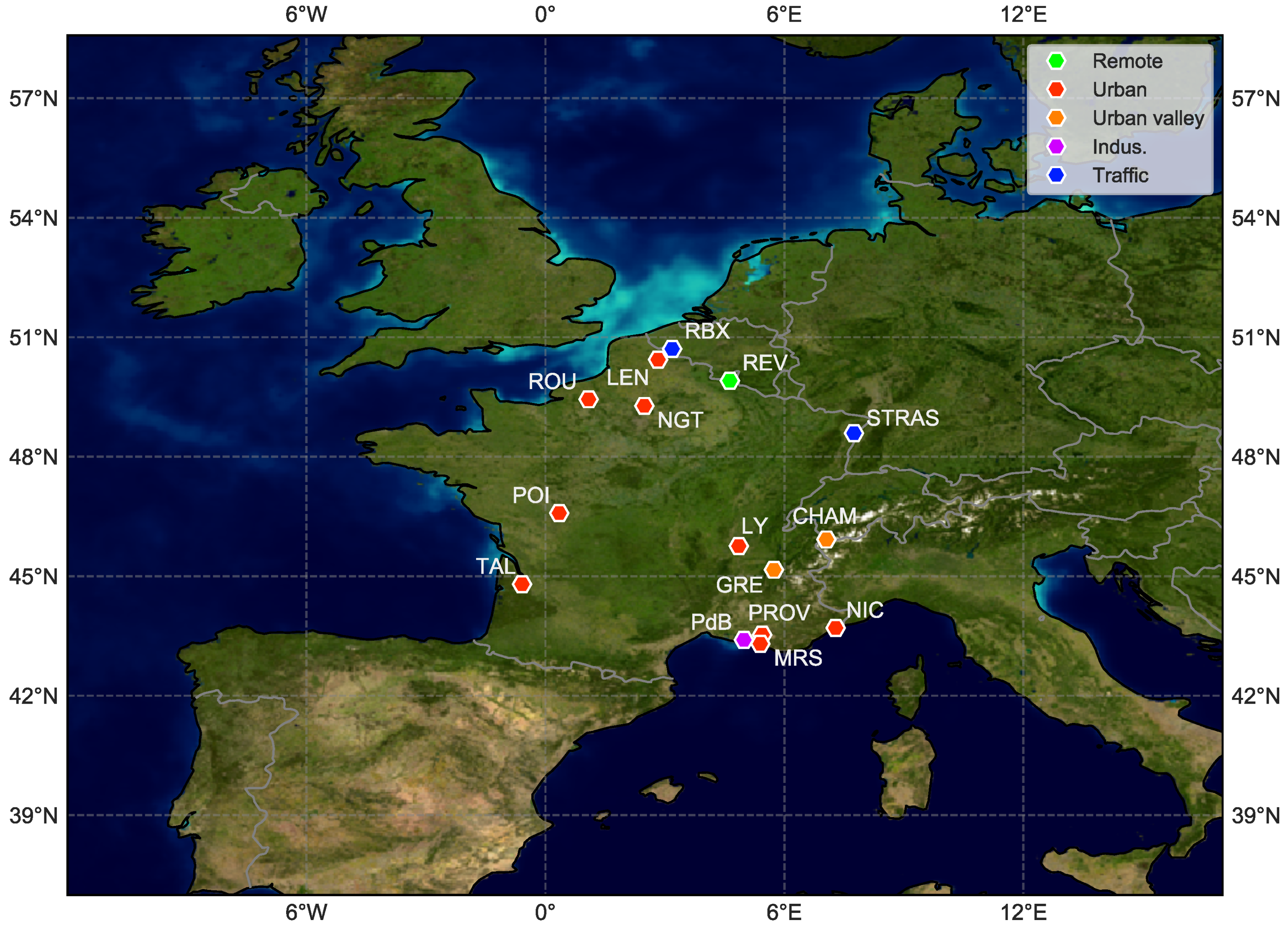
2.1. PM Sampling Sites

Figure 1 shows the geographical location of the 15 sampling sites for which comparable datasets (in terms of number of samples, investigated period and PM₁₀ chemical speciation data) were made available for the present study through the SOURCES project.

Table 1. Characteristics of the 15 PM sampling sites investigated in the present study.

Sampling Site	Code	Coordinates	Elevation	Period	N Samples	Typology
Revin	REV	49°55′00.00″N 4°38′29.00″E	395 m	2 Jan 2013→1 Jun 2014	168	remote
Bordeaux-Talence	TAL	44°48′ 2.01″N 0°35′17.01″W	20 m	2 Feb 2012→7 Apr 2013	154	urban background
Lyon	LY	45°45′27.82″N 4°51′15.15″E	160 m	3 Jan 2012→31 Dec 2012	115	urban background
Poitiers	POI	46°34′48.80″N 0°20′25.34″E	106 m	16 Nov 2014→29 Dec 2015	110	urban background
Nice	NIC	43°42′7.48″N 7°17′10.53″E	1 m	4 Jun 2014→29 Jun 2016	184	urban background
Marseille	MRS	43°18′18.84″N 5°23′40.89″E	64 m	11 Jan 2015→27 Jun 2016	102	urban background
Aix-en-Provence	PROV	43°31′49.04″N 5°26′29.00″E	180 m	18 Jul 2013→13 Jul 2014	56	urban background
Nogent sur Oise	NGT	49°16′35.00″N 2°28′56.00″E	28 m	2 Jan 2013→2 Jun 2014	155	urban background
Rouen	ROU	49°25′41.40″N 1°3′29.10″E	6 m	2 Jan 2013→1 Jun 2014	162	urban background
Lens	LEN	50°26′12.60″N 2°49′36.70″E	47 m	2 Jan 2013→1 Jun 2014	167	urban background
Grenoble	GRE	45°9′42.84″N 5°44′8.15″E	214 m	2 Jan 2013→29 Dec 2014	240	urban background & alpine valley
Chamonix	CHAM	45°55′21.00″N 6°52′12.00″E	1038 m	2 Nov 2013→31 Oct 2014	115	urban background & alpine valley
Port de Bouc	PdB	43°24′7.99″N 4°58′55.99″E	1 m	1 Jun 2014→27 Jun 2016	185	urban background & industrial
Roubaix	RBX	50°42′23.60″N 3°10′50.50″E	10 m	20 Feb 2013→26 May 2014	157	urban traffic
Strasbourg	STG	48°34′24.25″N 7°45′7.60″E	139 m	2 Apr 2013→8 Apr 2014	78	urban traffic

summarizes the characteristics of these sites. Most of them correspond to urban background stations and are distributed throughout France, including two Alpine cities (classified herewith as “Urban valley”). Other site typologies could also be investigated, with two urban traffic sites, one industrial, as well as one EMEP (European Monitoring and Evaluation Programme, https://www.emep.int/) rural background station.

At each site, PM₁₀ concentrations were monitored using automated analyzers, in accordance with recommendations of EN 16450:2017 [21], and daily (24 h) filter samples were collected every third day by employees of the corresponding regional air quality monitoring network. Samplings were achieved on pre-heated quartz fiber filters using high-volume sampler (DA80, Digitel), following EN 12341:2014 procedures [22]. Off-line chemical analyses performed on these filters are fully described in the Figure SI-1 of the Supplementary Materials. Briefly, the elemental and organic carbon fractions (EC and OC) were measured via thermo-optical analysis (Sunset Lab. Analyzer [23]) using the EUSAAR-2 protocol [24,25]. Major water-soluble inorganic contents (Cl⁻, NO₃⁻, SO₄²⁻, NH₄⁺, Na⁺, K⁺, Mg²⁺, and Ca²⁺) and methanelsulfonic acid (MSA) were determined using ion chromatography [25,26]). Many metals or trace elements (e.g., Al, Ca, Fe, K, As, Ba, Cd, Co, Cu, La, Mn, Mo, Ni, Pb, Rb, Sb, Sr, V, and Zn) were measured by ICP-AES or ICP-MS [27,28,29]. Finally, various anhydrosugars (including levoglucosan, mannosan, arabitol, sorbitol, and mannitol) were analyzed using High Performance Liquid Chromatography followed by pulsed amperometric detection (HPLC-PAD) [17].

2.2. PMF Methodology

2.2.1. PMF Model

The U.S. Environmental Protection Agency (US-EPA) PMF5.0 software [30] was used in the present study to achieve the PM source apportionment. Similar to other RM approaches, PMF aims at solving the mass conservation between the measured species concentrations and source emissions as a linear combination of factors p, species profile f of each source, and the amount of mass g contributed to each individual sample, following Equation (1):

$$X_{ij}=\left(\sum _p{g}_{ip}\times f_{pj}\right)+e_{ij}$$

(1)

where $X_{ij}$ represents the measured data for species j in sample i, and $e_{ij}$ is the residual of each sample and species not fitted by the model. Detailed information on the PMF methodology can be found elsewhere [8,9]. Briefly, a multivariate factor analysis was applied to decompose the matrix of the chemical dataset into two matrices: factor contributions (G) and factor profiles (F), each factor to be ascribed to a specific aerosol fraction (i.e., factor), that may be attributed to a source. It is based on a weighted least square fit, where the weights are derived from the analytical uncertainty, and provides the optimal solution by minimizing the function Q, given by Equation (2):

$$Q=\sum _i\sum _j{\left(\frac{e_{ij}}{{\sigma }_{ij}}\right)}^2$$

(2)

where ${\sigma }_{ij}$ represents the measurement uncertainty of each data point.

2.2.2. Input Variable and Uncertainties

Selection of the input variables was done based on the percentage of values above detection limit (DL) (using 60% as a minimum threshold), and the value of the signal-to-noise ratio (S/N) for each species [31].

Table 2. Input variables and uncertainties used in the PMF analyses.

	Carbonaceous Species	Water-Soluble Ions and MSA	Organic Markers	Metals and Trace Elements
Species	OC*, EC	MSA, Cl−, NO3−, SO42−, NH4+, K+, Mg2+, Ca2+	Polyols, levoglucosan, mannosan	Al, As, Ba, Cd, Co, Cr, Cs, Cu, Fe, La, Mn, Mo, Ni, Pb, Rb, Sb, Se, Sn, Sr, Ti, V, Zn
a coefficient	0.03	0.05	0.01	0.15

presents the PMF input variables selected for this work. This dataset notably includes EC, major ions, molecular organic markers (MSA, levoglucosan, and mannosan), and a selection of metals or trace elements. Assuming that they mainly originate from the same sources—i.e., primary biogenic emissions—sorbitol, arabitol and mannitol concentrations were summed and labeled as polyols [32]. Furthermore, OC* was determined by subtracting the carbon concentrations of the specific organic markers to total OC concentrations, so that they are not accounted twice:

$$O{C}^{*}=OC-(\left[MSA\right]\times 0.12+\left[polyols\right]\times 0.40+\left[levoglucosan\right]\times 0.44+\left[manosan\right]\times 0.44),$$

(3)

where the coefficient are the carbon mass par unit of mass.

The different variables were categorized in the model based on their mean signal-to-noise ratio (S/N) as follows: “strong” if $S/N>2$, “weak” if $0.2\le S/N\le 2$, and “bad” if $S/N<0.2$. For a given site, variables classified as “weak” were downweighted following PMF5.0 algorithms, while variables classified as “bad” were excluded from the PMF analysis. The PM₁₀ variable was classified as a total variable (with corresponding uncertainties increased by a factor of 3) to evaluate the contribution of the identified factors to PM₁₀ data. Extensive preliminary work was conducted to harmonize the estimation of uncertainties of the different input variables ${\sigma }_{ij}$, based on the uncertainty calculation equation proposed by Gianini et al. [33], as described by Equation (4):

$${\sigma }_{ij}=\sqrt{D{L}_j^2+{(C{V}_j\times x_{ij})}^2+{(a\times x_{ij})}^2}$$

(4)

with DL the detection limit (twice the standard deviation of field blanks, with field blanks samples representing about 5% to 10% of the actual number samples); $x_{ij}$ the concentration of species j on day i; CV the coefficient of variation of species j; and a the additional coefficient of variation.

Many trial-and-error tests were conducted with the aim of defining domains of variation of the coefficient a that are dependent on the type of analysis performed, i.e., to assign a a value to each category or family of chemical species analyzed. The PMF solutions obtained for different values of a were examined to optimize the stability of the results as well as the geochemical reality of the solved factors. The values eventually retained vary between 3% and 15% depending on the different categories of chemical species, as presented in Table 2.

It should also be noted that an uncertainty of $5/6\times DL$ was applied for values lower than the DL and uncertainties equal to four times the specie concentration geometric mean were attributed to missing or replaced values, following Polissar et al. [34].

2.2.3. Set of Constraints

One of the limitations of PMF is related to a possible collinearity of factors due to co-emission or co-accumulation phenomena, leading to rotational ambiguities. To solve this problem, specific chemical constraints based on expert geochemical knowledge can be applied to the chemical profiles (or contributions) of PMF factors (both “soft” and “hard” pulling, as defined in Section 3.4), after the selection of the initial base runs. As part of this study, a minimal and homogeneous set of chemical constraints was defined, as summarized in

Table 3. Summary of the specific constraints applied on source-specific tracers in some of the identified PMF factor profiles. SOA, secondary organic aerosol; HFO, heavy fuel oil.

Factor Profile	Species	Constraint	Value
Biomass burning	Levoglucosan	Pull up Maximally	%dQ 0.50
Biomass burning	Mannosan	Pull up Maximally	%dQ 0.50
Primary traffic	Levoglucosan	Set to 0	0
Primary traffic	Mannosan	Set to 0	0
Primary biogenic	Levoglucosan	Set to 0	0
Primary biogenic	Mannosan	Set to 0	0
Primary biogenic	Polyols	Pull up Maximally	%dQ 0.50
Primary biogenic	EC	Pull down Maximally	%dQ 0.50
Marine SOA	Levoglucosan	Set to 0	0
Marine SOA	Mannosan	Set to 0	0
Marine SOA	Polyols	Pull down Maximally	%dQ 0.50
Marine SOA	MSA	Pull up Maximally	%dQ 0.50
Marine SOA	EC	Pull down Maximally	%dQ 0.50
HFO combustion	Levoglucosan	Set to 0	0
HFO combustion	Mannosan	Set to 0	0
HFO combustion	Polyols	Set to 0	0
HFO combustion	MSA	Set to 0	0
Sea-salt	Ratio Mg2+/Na+	Sea-salt ratio 0.119	%dQ 0.50

. They were applied to the PMF analysis of each site.

2.3. Criteria for Valid Solutions

Solutions with a total number of factors from 6 to 12 were examined to capture the optimal number of factors for each site. Various statistical performance parameters to evaluate the robustness and relevance of the selected final solution were studied according to the recommendations of the European guide on air pollution source apportionment with receptor models [35], as well as the geochemical evaluation of the solution. Briefly, these parameters are summarized as follows:

• Evolution of the ratio Qtrue/Qrobust (<1.5). The solutions retained on all 15 sites have a Qtrue/Qrobust ratio of 1, indicating a zero impact of outliers on the results.
• The weighted residuals for most of the species have a normal centered distribution and between $\pm 4$, indicating an overall good modeling of most variables.
• Evaluation of the statistical representativity of the solution and sensitivity to noise and single point in the data from the bootstrap test (BS) for 100 successive iterations of the model and for a minimum correlation $r^2$ of 0.6.
• Evaluation of the rotational ambiguity and sensitivity of the solution to small changes from (default dQ of the software) the Displacement Test (DISP) proposed by the software.
• Evaluation of the geochemical meaning and the physical reality of extracted factor profiles based on the knowledge of the chemical footprints of the sources, their specific tracers, the temporal variability (daily, weekly and seasonally), and the characteristics of the site studied.
• Statistical evaluation and precision for constrained solutions regarding the BS and %dQrobust as well as DISP.

Further discussions on the BS and DISP approaches are proposed in Section 3.4.

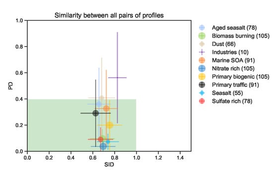
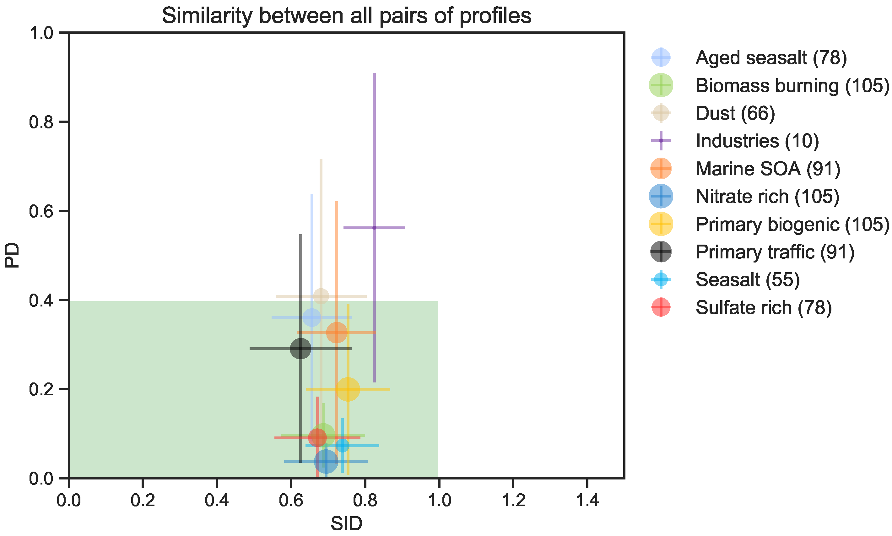
2.4. Test of Similarity between Chemical Profiles

Since factors in the different PMF were labeled with the same name due to their chemical composition and time variation, a tool was needed to objectively assess the homogeneity of their chemical profiles. The similarities between the factors or sources were tested with both the Pearson distance (PD) and the Similarity Identity Distance (SID), following Belis et al. [36] and using Python 3.5. The PD is equal to $1-r^2$ where $r^2$ is the Pearson coefficient and SID is defined by Equation (5):

$$SID=\frac{\sqrt{2}}{m}\sum _{j=1}^m\frac{|x_j-y_j|}{x_j+y_j},$$

(5)

with x and y the relative mass to the PM of two different factors or sources and m the number of common specie in x and y.

Shortly, these two metrics aim to compare two profiles based on their common chemical relative mass composition. The PD is highly sensitive to variation in the major mass fractions of the PM, while the SID is equally sensitive to all components. $PD<0.4$ and $SID<1$ are considered as acceptable criteria for profile similarity, according to Pernigotti and Belis [37].

3. Results and Discussions

The outputs of the SOURCES project consist of a large database, which cannot be exhaustively discussed in a single paper. Here, we present an overview of obtained PMF’s results, give some examples of factor’s behaviors, and focus on the statistical evaluation of the solutions as well as on the comparability of various factors. However, all the results—including time-series and factors profiles along with their corresponding uncertainties—have been made interactively available online at http://pmsources.u-ga.fr. This application is proposed as Supplementary Materials for the present paper.

It should be noted that the harmonized methodology used for the purpose of this study may lead to slight discrepancies when compared to results obtained in the case of PMF analysis performed specifically at a given site, as discussed for instance in Favez et al. [38].

3.1. Identification of Factors

The number of selected factors varied between 8 and 11 depending on the site. Among these factors, nine were identified at most of the locations: biomass burning, exhaust and non-exhaust road transport emissions (primary traffic), secondary aerosols dominated by ammonium nitrate and ammonium sulfate (nitrate-rich and sulfate-rich, respectively), primary biogenic particles, secondary organic aerosols (SOA) from marine biogenic emissions (marine SOA), fresh and/or aged sea-salt, and mineral dusts. It is noteworthy that this harmonized methodology enables identifying such a large and common set of factor at the national scale. Two other minor factors were exclusively identified at a few sites and seem to be specific of local sources: industrial emissions (at five sites) and emission related to combustion of heavy fuel oil (HFO) (at three sites).

All of these chemical profiles were identified and attributed to different sources (or source categories) mainly based on the presence of specific chemical tracers or combination of markers, as presented in

Table 4. Summary of the characteristic marker species used to identify PMF factors.

Identified Factors	Specific Markers and Indicators
Biomass burning	Levoglucosan, mannosan, K+, OC, EC
Primary traffic	EC, OC, Ba, Cr, Co, Cu, Fe, Mo, Pb, Sb, Sn, Zn
Nitrate rich	NO3−, NH4+
Sulfate rich	SO42−, NH4+, Se, OC
Primary biogenic	Polyols
Marine SOA	MSA
Dust	Ca2+, Al, Ba, Co, Cu, Fe, Mn, Pb, Sr, Ti, Zn
Sea-salt	Na+, Mg2+, Ca2+, Cl−
Aged sea-salt	Na+, Mg2+, NO3−, SO42−
Industries	As, Cd, Cr, Cs, Co, Ni, Pb, Rb, Se, V, Zn
Heavy fuel oil (HFO)	V, Ni, SO42−, EC

. In some cases, it was impossible to separate two factors among the ones listed in Table 4, and they were named as a combination of both of them (Figure 2). The main chemical characteristics of the factors identified at all 15 sites, as well as the particularities observed on some sites, may be found in the web app, together with their concentrations time series.

One of the specificities of theses PMF is the use of organics species (polyols and MSA notably). Discussion on the identification of the factors may be found in previous paper [4,17,39,40,41,42], where the same criteria are applied. However, we would like to mention the presence of Se in the sulfate rich factor. Indeed, Se is not often used in PMF studies together with organics. In this study, 23 ± 15% of the Se was associated to the sulfate rich factor, together with 13 ± 6% of the OC*. Such association of Se, SO₄²⁻ and OC is already documented for soil [43] as well for the emission of Se and S from marine algae [44]. It has also been reported that abiotic condition could lead to the formation of volatile Se when associated with organic acid [45,46,47]. Then, the sulfate rich factor may not be only an inorganic aerosol but may also be induced by the formation of secondary organics.

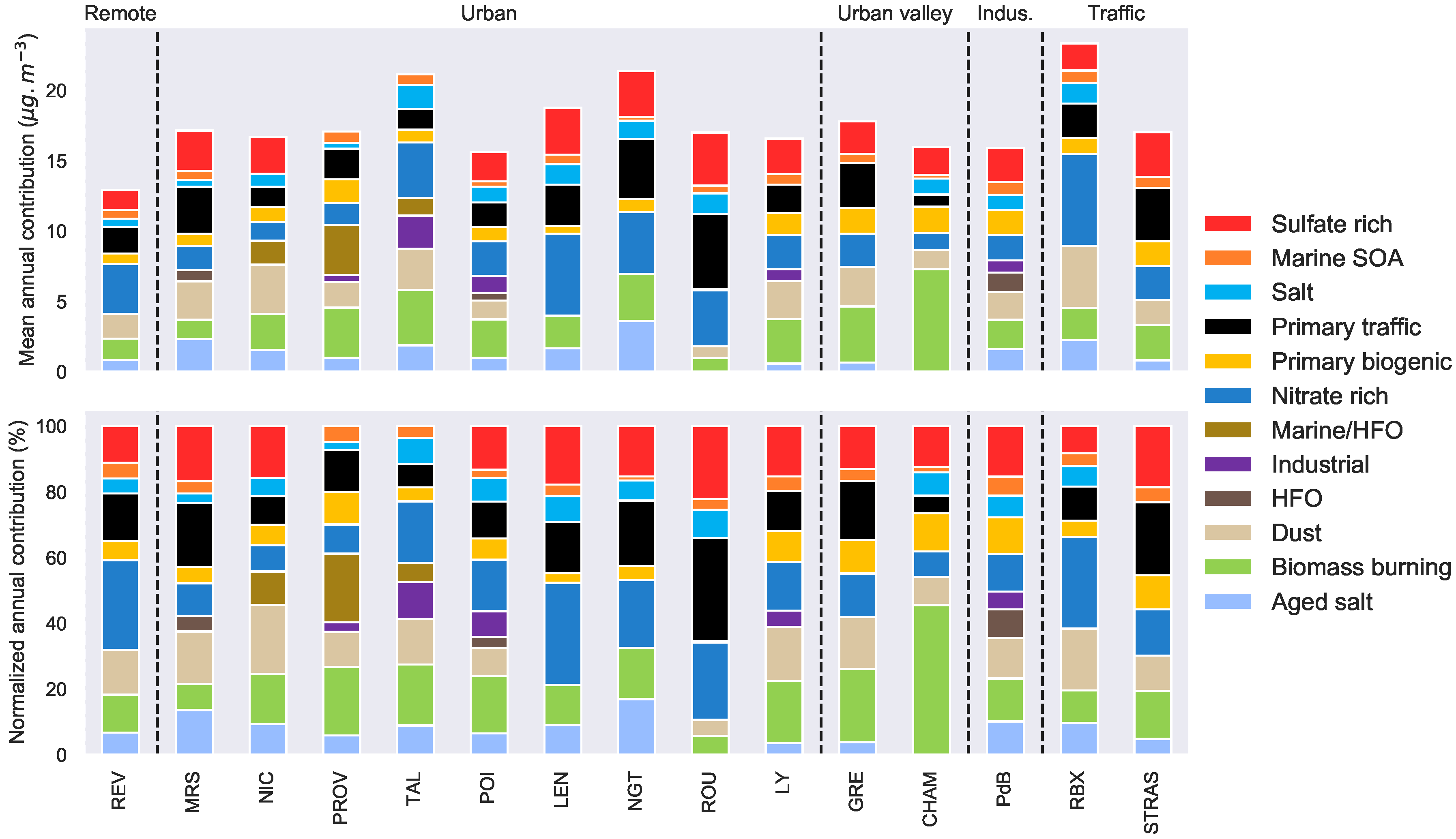
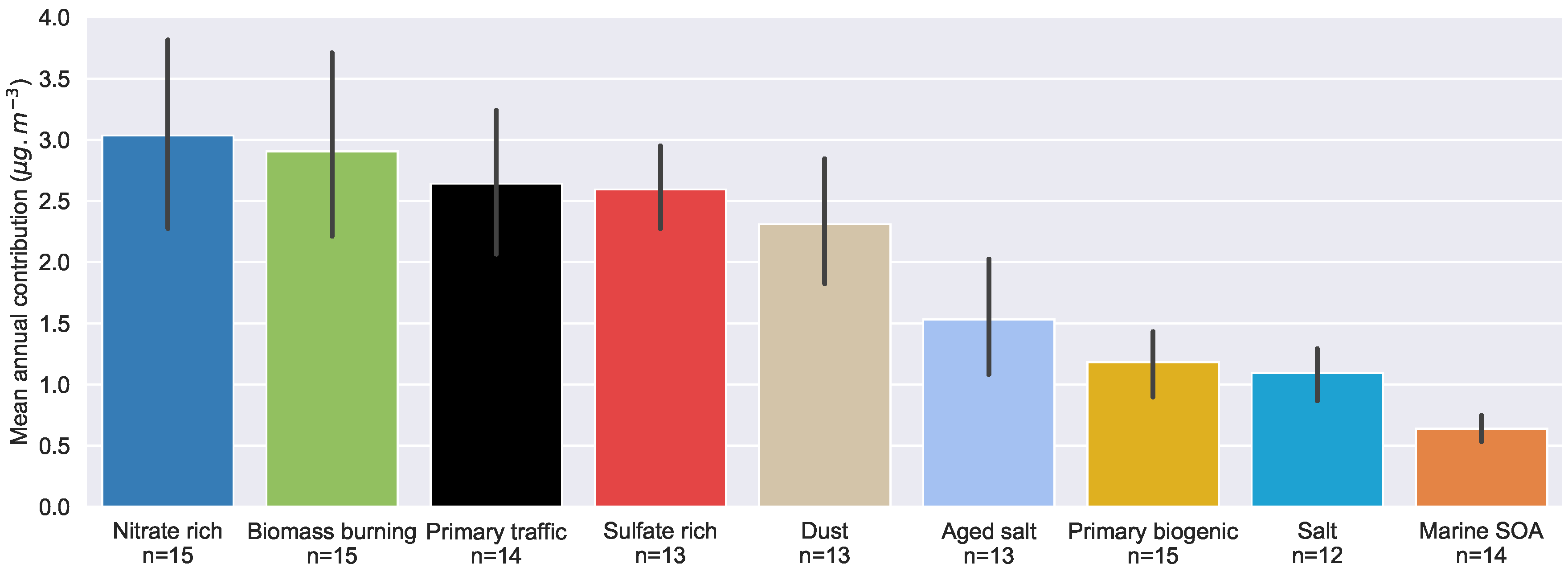
3.2. Major Source Contributors to PM

Figure 2 presents the yearly mass contributions of the different factors identified at all sites, in both absolute (top) and relative (bottom) contributions. The all-sites average ranked contributions of the main PM factors are presented in Figure 3.

The average concentration of PM₁₀ for each site ranged from $13.0$ $\mathsf{\mu }$$\mathrm{g}$ ${\mathrm{m}}^3$ for the rural site of REV to $23.3$ $\mathsf{\mu }$$\mathrm{g}$ ${\mathrm{m}}^3$ for the traffic site of RBX, with an average concentration of $17.6\pm 2.6$ $\mathsf{\mu }$$\mathrm{g}$ ${\mathrm{m}}^3$. As already pointed out in previous recent studies conducted at French sites [4,16,17,39,48,49], one of the main PM factor is biomass burning, with an average contribution of $2.9\pm 1.5$ $\mathsf{\mu }$$\mathrm{g}$ ${\mathrm{m}}^3$ (17 ± 9% of PM₁₀ mass), coming mainly from residential heating. This is particularly true for Alpine valley sites, as exemplified with the CHAM site in this study, where it reaches 45% of the total PM₁₀ mass (Figure 2). We also clearly observed the large contributions of PM₁₀ formed through secondary processes, namely the nitrate-rich and the sulfate-rich factors, representing on average $3.0\pm 1.6$ $\mathsf{\mu }$$\mathrm{g}$ ${\mathrm{m}}^3$ (17 ± 8%) and $2.6\pm 0.7$ $\mathsf{\mu }$$\mathrm{g}$ ${\mathrm{m}}^3$ (15 ± 4%), respectively. Since such factors impact all of the metropolitan France territory, it suggests the importance of large-scale processes at the European scale, especially during PM pollution events in the late winter-early spring period [4,50,51]). The primary traffic factor represents another important fraction, with a yearly contribution of $2.6\pm 1.2$ $\mathsf{\mu }$$\mathrm{g}$ ${\mathrm{m}}^3$ (15 ± 7%). It should be noted that this factor was assessed to comprise oxidized compounds formed rapidly after emission, but to miss some of the secondary species (e.g., ammonium nitrate, SOA) partly originating from precursors and/or oxidative species within exhaust smoke, such as high-volatility organic and nitrogen gaseous compounds. As another primary anthropogenic source, a pure HFO factor was observed for only three locations, with the highest contribution to PM₁₀ (about 5%) at the industrial site of PdB. Finally, some industrial related PM was found at five sites, but the exact types of industrial activity were not identified.

Considering natural particles, the dust factor was identified as a large contributor at almost all sites ($n=13$), representing on average $2.3\pm 1.0$ $\mathsf{\mu }$$\mathrm{g}$ ${\mathrm{m}}^3$ (13 ± 4%). However, this latter factor could possibly be considered as a mixing between terrigenous aerosols and mineral particles linked to human activities (e.g., building works, resuspension due to road transport, etc.), since it includes variable amounts of trace elements depending on the site. The primary biogenic and marine SOA factors—traced by polyols and MSA, respectively—represent $1.2\pm 0.5$ $\mathsf{\mu }$$\mathrm{g}$ ${\mathrm{m}}^3$ ( 7 ± 3%) and $0.6\pm 0.2$ $\mathsf{\mu }$$\mathrm{g}$ ${\mathrm{m}}^3$ (4 ± 1%) on a yearly average and display the lowest dispersion among all the sites studied, suggesting common large-scale processes for these two factors. An extensive discussion on the primary biogenic factor for these sites can be found in Samaké et al. [32]. The fresh sea-salt fraction display an average concentration of $1.1\pm 0.4$ $\mathsf{\mu }$$\mathrm{g}$ ${\mathrm{m}}^3$ (6 ± 2%) while the aged sea-salt factor was observed at almost all sites, with an average concentration of $1.5\pm 0.9$ $\mathsf{\mu }$$\mathrm{g}$ ${\mathrm{m}}^3$ ( $8\pm 4$%) (Figure 3). This last result strengthens the importance of the secondary processes that occurs during the aging of natural aerosols, possibly leading to internal mixing with anthropogenic emissions. Similarly, a marine/HFO factor—notably containing sulfate, vanadium, sodium and chloride—was observed at three coastal sites, pointing to substantial influence of shipping emissions at these sites.

3.3. Seasonality of the Contributions

Since it is not possible to present all the results in this paper, we encourage the reader to refer to the online view app to browse the different time series and chemical profiles. Among the factors that present a strong seasonality (nitrate rich, biomass burning, primary biogenic and marine SOA) we choose to highlight the seasonal contributions of the biomass burning (main contribution during winter) and the primary biogenic (main contribution during summer) (Figure 4 and Figure 5, respectively).

With about 35% of the PM₁₀ mass during winter and less than 2% during summer (see Figure 4), the biomass burning factor shows the strongest seasonality among all factors identified. At the two sites investigated in the Alpine valley, and due to frequent inversion layers in winter, the contribution of the biomass burning can reach up to 70% of the total PM₁₀ mass in the cold season, as already mentioned in previous studies in the Alps [4,52,53,54].

Conversely, the primary biogenic factor can contribute to a significant amount of PM₁₀ during the warm months, with an average contribution to PM₁₀ of 13 ± 8% (min 1.5%, max 33% among the sites studied) during summertime, as shown in Figure 5. A detailed study about the seasonal and spatial variations of the primary biogenic factor resulting from these PMF analyses can be found in Samaké et al. [32].

3.4. Uncertainties of PMF Factors

In factor analysis, three sources of uncertainties can arise from: (1) random errors in data values linked to measurement uncertainties: (2) rotational ambiguity due to possible multiple acceptable solutions; and (3) modeling errors, such as mis-specification of the model compare to the real processes in atmosphere [35].

To quantify the uncertainties of the results at one site (internal uncertainties), and the variability of the factor profiles, we performed both bootstrap (BS) and displacement (DISP) analyses. Shortly, BS randomly resample the X matrix and perform a new PMF run, then try to map each new BS-factor to the reference run, according to the correlation between the contributions of factors. A threshold correlation coefficient of 0.6 was used for all sites in this study. BS gives an estimation of uncertainties linked to sampling artifact and measurement uncertainties. DISP analysis estimates the rotational ambiguity by lowering and majoring each species in every factor up to a given variation of the Q value dQmax. The reader may refer to Paatero et al. [20] for more details about DISP computation in EPA PMF5.0. Here, BS and DISP analyses were applied in both base runs and constrained runs, i.e., before and after applying the constraints listed in Table 3.

3.4.1. Statistical Stability of the Solutions

In this study, all base cases solutions (i.e., without constraints) reached high BS values, the lowest one being 77% (

Table 5. Summary of bootstrap mapping of the base runs and of the constrained runs expressed as percent of correct mapping bootstrap for the main factors identified in this study. Ranges are min and max. The number in parenthesis is the number of sites where the given profile could be identified.

Profiles	Base Cases			Constrained Cases
	Mean ± Std	Range	Unmapped	Mean ± Std	Range	Unmapped
Biomass burning (15)	100.0 ± 0.0	100–100	0.0	100.0 ± 0.0	100–100	0.0
Nitrate rich (15)	98.7 ± 2.8	89–100	0.2	99.9 ± 0.3	99–100	0.0
Primary biogenic (15)	99.3 ± 1.3	96–100	0.0	99.8 ± 0.8	97–100	0.0
Marine SOA (14)	95.9 ± 4.9	83–100	0.7	100.0 ± 0.0	100–100	0.0
Primary traffic (14)	97.1 ± 4.8	85–100	0.0	98.7 ± 2.8	89–100	0.0
Aged sea-salt (13)	95.8 ± 4.8	83–100	0.1	98.5 ± 2.7	91–100	0.1
Sulfate rich (13)	93.4 ± 6.9	83–100	0.5	98.9 ± 1.8	95–100	0.1
Dust (12)	94.1 ± 7.3	77–100	0.7	97.8 ± 4.8	83–100	0.1
Sea-salt (11)	99.5 ± 1.5	95–100	0.0	99.8 ± 0.6	98–100	0.0
Industries (5)	92.8 ± 8.5	80–100	1.0	98.4 ± 2.2	96–100	0.0

). Hence, the PMF base solution for all sites already presents very good BS mapping results that largely agree with the general recommendations of the European guide on air pollution source apportionment with receptor models [35]. Moreover, we systematically observed improvement in BS mapping when applying constraints (Table 5). Considering all the sites, the minimum value of BS for constraint solutions was 83%. It means that, even if the base cases were good enough to differentiate specific factors, the expert knowledge added through the use of specific constraints helped the model to “clean” the factors and improve the stability of the solutions. Finally, we note that virtually no “unmapped” factor was obtained during this BS sensitivity analysis (always less than 1%). Concerning the DISP analyses, no swap between factors was observed, for both the base and constrained runs.

3.4.2. Uncertainties of the Profile Composition

Impacts of the Constraints on the Uncertainties

The application of specific chemical constraints (see Table 5) also improved the resolving power of the PMF and the quality of the solutions, displaying narrower uncertainties for the contributions of chemical species in many factors. For instance, the OC* concentration in the primary traffic profile of ROU varied between 0.79 and $1.65$ $\mathsf{\mu }$$\mathrm{g}$ ${\mathrm{m}}^3$ for the base run but only between 1.23 and $1.84$ $\mathsf{\mu }$$\mathrm{g}$ ${\mathrm{m}}^3$ in the constrained run, according to the BS analysis (5th–95th) (

Table 6. Summary of the uncertainties (in $\mathsf{\mu }\mathrm{g} {\mathrm{m}}^3$) obtained from the BS (5th and 95th percentiles) and DISP (min-max) runs for a subset of species in two different factor profiles, the road traffic at ROU site and the biomass burning at GRE site, for both the base and constrained runs.

	ROU—Primary Traffic
Run	Base				Constrained
Species	OC*	EC	Cu	Fe	OC*	EC	Cu	Fe
Reference	1.605	0.541	0.0104	0.1986	1.649	0.592	0.0114	0.221
BS (5th–95th)	0.792–1.654	0.334–0.541	0.007–0.011	0.108–0.232	1.232–1.845	0.493–0.641	0.009–0.013	0.159–0.264
DISP (min-max)	1.426–1.912	0.480–0.644	0.009–0.012	0.178–0.229	1.576–1.837	0.572–0.666	0.011–0.012	0.210–0.236
	GRE—Biomass Burning
Run	Base				Constrained
Species	OC*	EC	Levoglucosan	K+	OC*	EC	Levoglucosan	K+
Reference	1.266	0.434	0.306	0.057	1.520	0.563	0.388	0.059
BS (5th–95th)	1.061–1.505	0.372–0.614	0.269–0.362	0.039–0.067	1.347–1.640	0.492–0.672	0.412–0.434	0.039–0.070
DISP (min-max)	1.100–1.363	0.378–0.480	0.275–0.319	0.050–0.061	1.456–1.589	0.539–0.604	0.408–0.439	0.058–0.059

). Similar trends were observed for the uncertainties proposed by the DISP approach and were apparent for most of the chemical species that are proxies of a given source (Table 6 proposes some examples).

Interestingly, the uncertainties estimated with the DISP method were almost always narrower than the uncertainties given by the BS method. This may be explained by using constraints that already narrowed the rotational ambiguity (lowering DISP uncertainties range) or by the sensitivity of our datasets to specific days (increasing BS uncertainties range).

Composition Uncertainties in the Chemical Profiles

The dispersion of the concentrations of key species in different profiles was investigated and is briefly presented here. The external variability (from site to site) is presented in its own section below (Section 3.6). Here, we only assessed the internal variability, i.e., the variability of a specie at a given site for a given factor, and the coefficients of variation (CV, standard deviation over the mean) of species from the BS runs are presented in Figure 6, averaged from all sites. To minimize the impact of potential outliers in the BS runs, only the BS values above the 5th percentile and below the 95th percentile were used.

For most of the main proxies of sources (i.e., specific tracers), we observed a narrow range of possible values given by the BS and DISP, associated with low CV for the specific tracers. This is the case for instance for the levoglucosan in the biomass burning factor (1.6 ± 0.5%), the MSA in the marine SOA (1.2 ± 0.8%), the polyols in the primary biogenic (0.1 ± 0.1%), the Ti in the dust (12.2 ± 9.6%), the Na+ in the sea-salt (10.3 ± 7.2%), NO₃⁻ in the nitrate rich (6.5 ± 2.5%) or even Cu and Sb in the primary traffic (14.0 ± 11.0% and 16.0 ± 12.4%, respectively, which are the lowest CVs for these two metals for all factors).

However, for non-tracers species, the dispersion according to the BS and DISP runs could be larger. For instance, according to BS, the OC* and Ca²⁺ in the nitrate rich have a CV of 60.4 ± 35.9% and 59.6 ± 39.1%, respectively, or the metals in the primary biogenic factor.

We also note that some species have an extremely large CV in some factors, notably the NO₃⁻ in the sulfate rich factor (354.3 ± 301.3%). This likely indicates some possible mixing with other factor or more generally the fact that the PMF model did not find a well defined solution for this species in this factor. Conversely, we can see in Figure 6 that the main species with regard to the mass are stable in the biomass burning factor. Notably, PM₁₀, OC* and EC had CVs of 12.2 ± 6.8%, 12.8 ± 8.9% and 25.6 ± 22.9%, respectively, an indication that the components of this factor were well described by the PMF run.

Therefore, despite high confidence in the markers and in the obtained mass fractions, caution should be taken when scrutinizing the repartition of a given species between factors and extrapolating specific ratio if the species present some large uncertainties.

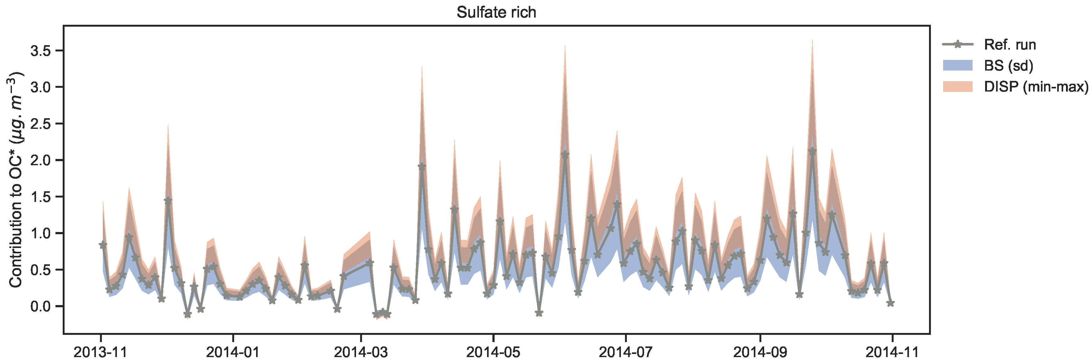
3.5. Estimation of the Uncertainties of Time Series Concentrations

This section presents an attempt to express the uncertainties associated with the concentrations of a chemical species in the time series of a specific factor contribution. Even if during the BS runs both the F and G matrices were recomputed, only the F matrix was returned to the user in the EPA PMF5.0 software. The matrix G was only used internally to map the BS factor to the base factor [20]. As a result, the outcome was an estimation of uncertainties for the F matrix, but not for the G one. Hereafter, we propose to estimate the uncertainties for the time series of the concentrations of a chemical species by multiplying the different concentrations given by the uncertainties runs (BS and DISP) by the factor contribution of the reference run $G_{ref}$:

$$X_{ERRi}^{\prime }=F_{ERRi}·G_{ref},$$

(6)

where $F_{ERRi}$ refers either to the F matrix given by the DISP min/max run or to one of the BS runs, $G_{ref}$ is the contribution matrix of the reference run, and $X_{ERRi}^{\prime }$ simulates the temporal concentration of species in the run $ERRi$ (DISP or BS). It should be noted that this method only represents an approximation of the “true” uncertainties of the model over the sample time series. Indeed, both the F and G matrix should theoretically be modified at the same time, whereas the different $F_{ERRi}$ were multiplied here by a constant value of G for a given sample. Therefore, samples with high concentration (G) will always have higher uncertainties than sample with low concentration.

However, this method provides a first idea of the uncertainties in the time series and help to visualize the uncertainties given by the BS and DISP methods. For instance, uncertainties (i.e., standard deviation of BS, and DISP min/max) of the OC* in the sulfate-rich factor obtained for the site CHAM are presented in Figure 7, coupling the uncertainties in the chemical profile (OC*_ref, $0.5423$ $\mathsf{\mu }$$\mathrm{g}$ ${\mathrm{m}}^3$; OC*_BS, $0.568\pm 0.262$ $\mathsf{\mu }$$\mathrm{g}$ ${\mathrm{m}}^3$; and OC*_DISP, 0.612$\mathsf{\mu }$$\mathrm{g}$ ${\mathrm{m}}^3$–0.934$\mathsf{\mu }$$\mathrm{g}$ ${\mathrm{m}}^3$) and the concentrations time series. In this example, it may be hypothesized that the sulfate-rich factor may be mixed with another aerosol fraction (e.g., possibly SOA) since it presents some important uncertainties and high concentration of OC* during summertime. Even if it may be possible by directly tweaking the ME-2, the solver used in EPA PMF5.0 software, it seems difficult for the non-computers-scientist end-user to extract the different G matrices. We think that an added value to the software would be to output them during the BS process and we encourage developers of other PMF software to ease this process.

3.6. Variability of the Chemical Profiles at the Regional Scale

3.6.1. Overall Comparison

In the previous sections, we discuss the internal variability of the different factors. Next, similarities of all the chemical profiles identified in this study were investigated thanks to the tools developed in the frame of the FAIRMODE (Forum for Air Quality Modeling) activities and presented by Belis et al. [36], based on the constrained runs. PMF factor profiles attributed to a source category are compared among each other’s using both the PD (Pearson distance) and SID (standardized identity distance) similarity indicators. Fewer factors identified at some sites were not considered in this assessment analysis as they showed some mixing with other emission sources.

Figure 8 gives mean and standard deviation of the distances between all pair of factor/source profiles tagged as belonging to the same category in the SID-PD space. It results in the comparison of $n\times \frac{n+1}{2}-n$ pairs of profiles for each category, where n is the number of profiles belonging to the same source category (see Figure 8).

First, we can see that many factor/source profiles present low PD and SID with values (mean ± standard deviation) inside the acceptance box ($PD<0.2$ and $SID<0.8$), indicating that they are stable over the different sites of the study. It includes the biomass burning, sulfate-rich, nitrate-rich, and fresh sea-salt factors. The primary biogenic source also appears relatively stable at all sites but presents some dissimilarity according to the PD metric. It suggests that this source is not yet fully understood and need further investigation, as recently discussed by Samaké et al. [32].

Other factors seem to have more heterogeneous profiles, with part of their values (mean ± standard deviation) outside of the acceptance box. For instance, differences were clearly observed in the few industrial chemical profiles. This is expected as such emissions may be very local and highly variable, despite their common contents of high concentrations of metals and metalloids. Marine SOA profiles also display site-to-site variations and a wide range in the PD-SID space, notably for the PD metric. This factor, mainly identified thanks to its MSA marker, may actually regroup a large diversity of chemical species. The low variance in the SID but high variance in the PD tends to indicate a large discrepancy for the chemical species that represent the main mass of the profile. A deeper analysis (not presented here) showed that the high variance is driven by an observation at only three sites: GRE, CHAM and ROU. The valley sites of GRE and CHAM both present a larger part of OC* in their profile while, conversely, ROU presents the lowest amount of OC* among all the sites. Finally, the primary traffic profile presents the lowest SID values, but a relatively high PD, still in the acceptable area. As this factor is commonly observed in RM studies and contributes substantially to the PM₁₀ mass, it is discussed in detail in the following section.

3.6.2. A Non-Homogeneous Source: Primary Traffic

The primary traffic source present large variability in the SID-PD space, suggesting a wide variety of road transport chemical profiles over France. As a matter of fact, this factor presents the lowest SID value of all profile while larger variabilities were found in the PD metric. This could be seen in the OC/EC ratio, both species being the most abundant ones within the primary traffic factor (Figure 9 and Figure 10). Even when excluding the rural site of REV, we observed a large variability in this ratio, spanning from 0.09 to 3.31 (Figure 10). As the PD is mainly sensitive to the main chemical species in term of mass, these two compounds may explain the wide span of the PD value for this source. It should also be noted that the high variability in the PD may be driven by the values for the RBX site. Indeed, despite RBX has all 22 metals in the ranges of the other sites, the value of OC* is extremely low compared to others sites. The lower dispersion in the SID-axis highlights the relative homogeneity of the other components of this factor. Indeed, as shown in Figure 9, the amount of metals, notably the Fe, Cu, Al, Zn and Sb, as well as sulfate are relatively homogeneous over the 14 sites. We also see that organic compounds such as levoglucosan, mannosan, MSA and polyols as well as Na⁺ are almost never present in this factor, or in a very small amount.

The extremely high OC-to-EC ratio for REV (Figure 10) and the relatively higher uncertainties estimated from the BS runs (OC*_BS, 0.000$\mathsf{\mu }$$\mathrm{g}$ ${\mathrm{m}}^3$–0.937$\mathsf{\mu }$$\mathrm{g}$ ${\mathrm{m}}^3$; EC_BS, and 0.0162$\mathsf{\mu }$$\mathrm{g}$ ${\mathrm{m}}^3$–0.0703$\mathsf{\mu }$$\mathrm{g}$ ${\mathrm{m}}^3$, still close to the detection limit) indicate low confidence in the PMF solution for this factor at this site.

Finally, the primary traffic factor is the closest to the dust factor when comparing the dust factor to all other profiles (see Figure S1). Such results may indicate that some resuspended dust coming from road abrasion or resuspension might contribute importantly to the dust factors at some sites. This may also explain the relatively low amount of trace element in the primary traffic factor obtained at STRAS. Indeed, at this site, we identified a mixed factor of “resuspended dust”, which may be a mixing between mineral dust and road dust. This particular factor is not included in the “dust” one presented in Figure 8 due to it singularity.

3.7. A Homogeneous Source: The Biomass Burning Source

Among the stable profiles, the biomass burning is the most important source in terms of mass contribution. As already well reported in the literature [6,55,56], OC is the PM dominant fraction in this source, with a quite constant amount (38 ± 5% of the PM mass, see Figure 11). Moreover, as presented in Figure 6 and detailed in Figure S2, the OC* uncertainties in this factor is low. Concerning the tracer of biomass burning, levoglucosan and mannosan are present at 96 ± 3% and 95 ± 4% in this profile, respectively (Figure 11). Mass-wise, the levoglucosan represents 8 ± 2% of the total PM mass. The EC presents a wider dispersion, with a mass concentration of 9 ± 4%. We also note a fair amount of Cl⁻, as well as K⁺ in this factor, which explains 14 ± 19% and 32 ± 13% of their respective total mass. Despite its contribution to the mass of biomass burning PM mass (6 ± 4%), the NO₃⁻ is clearly not mainly allocated to this source as the biomass burning represents only 7 ± 5% of the total NO₃⁻ mass. Metal elements are barely present in this factor and some high discrepancy was observed for the different sites, with a dispersion up to two orders of magnitude for Pb, Zn and Mn. It may be noted that the OC-to-Levoglucosan ratio fluctuates between 2.1 and 7.4, with a mean and standard deviation values of 4.61.5 (Figure 10). Such ratios are in the 1.9–12.6 range of values previously reported for PM₁₀ wood combustion samples [55,56]. They may reflect the use of the different type of wood for heating purposes, as detailed in the same previous studies. However, we did not observe any systematic difference according to the geographical location and/or the site typology for this source. Overall, these findings suggest a relatively similar wood burning emission in term of PM constituents all over the territory.

4. Conclusions

This paper presents results obtained from PMF analyses conducted in a harmonized way and taking advantage of datasets corresponding to more than 2200 samples collected at 15 different sampling sites in France. To the best of our knowledge, this is the first study using such a large database over several years of monitoring. Thirty-seven input variables were selected to cover a wide range of major expected PM₁₀ factors and to optimize total mass reconstruction at all sites. The operator-related subjectivity was reduced by using homogeneous statistical and geochemical criteria for the source discrimination and identification.

Overall, the main PM₁₀ factors were found to be primary traffic (15 ± 7% of the PM₁₀ mass on a yearly average) and biomass burning (17 ± 9%) as well as two secondary aerosol fractions dominated by ammonium nitrate (17 ± 8%) and ammonium sulfate (15 ± 4%), respectively. These findings are in good agreement with what has commonly been observed by many previous studies over Europe and illustrates—if still needed—the major impact of anthropogenic emissions on urban air quality. Nevertheless, substantial contributions of mineral dusts (13 ± 4%), fresh (6 ± 2%) and/or aged sea-salts (8 ± 4%), as well as of primary biogenic aerosols (7 ± 3%) are also observed at almost all sites, reflecting that natural emissions should not be neglected as other important contributors to PM₁₀ levels on a yearly basis.

During wintertime, high contribution of the biomass burning was observed, together with the nitrate-rich factor in early spring (March). The sea-salt also presents higher contribution during this period of the year, potentially linked to stronger westerlies winds. In summer, all sites present important contributions from biogenic sources: the primary biogenic and marine SOA factors. Conversely, the primary traffic, dust, aged sea-salt and sulfate rich factors do not present clear seasonality pattern. Uncertainties of each PMF results were investigated thanks to the bootstrap and displacement methods, both for the base and the constrained runs. The use of a set of constraints—taken as limited as possible—allows to decrease these uncertainties and to strengthen the output statistical representativity of factors commonly observed all over the French continental territory. The internal variability (i.e., for a given site) assessment shows high confidence for the concentration of the main proxies of sources (i.e., specific tracers) and for the PM₁₀ mass apportionment, but larger uncertainties were found for concentrations of non-tracer species and caution should be taken concerning the contributions of such chemical species to the different factors.

Finally, the external variability (i.e., from one site to another) was investigated thanks to both the SID and PD metrics. In particular, the discrepancy between the chemical profiles of sources could be quantified thanks to both the SID and PD metrics, notably showing that fresh sea salt, nitrate-rich, sulfate-rich and biomass burning factor profiles can be considered as chemically similar at all the sites studied. Conversely, some significant variabilities were observed for other factor chemical profiles, such as the ones related to traffic and industrial emissions as well as mineral dusts and marine SOA. The latter finding is calling for the use of additional variables, such as organic molecular markers, within studies aiming at scrutinizing specific local sources at individual sites and/or for a better knowledge on the origins of SOA fractions.

Overall, results obtained in this comprehensive study may help to increase the completeness of the SPECIEUROPE database, and can be used to assess the contributions of the different sources to the oxidative potential of PM₁₀ following methodology proposed by Weber et al. [49].

References

1. IPCC. Climate Change 2013: The Physical Science Basis; Contribution of Working Group I to the Fifth Assessment Report of the Intergovernmental Panel on Climate Change; Technical Report; IPCC: Cambridge, UK; New York, NY, USA, 2013. [Google Scholar]
2. Kelly, F.J.; Fussell, J.C. Linking ambient particulate matter pollution effects with oxidative biology and immune responses: Oxidative stress, inflammation, and particulate matter toxicity. Ann. N. Y. Acad. Sci. 2015, 1340, 84–94. [Google Scholar] [CrossRef] [PubMed]
3. Lippman, M.; Chen, L.C.; Gordon, T.; Ito, K.; Thurston, G.D. National Particle Component Toxicity (NPACT) Initiative: Integrated Epidemiologic and Toxicologic Studies of the Health Effects of Particulate Matter Components; Technical Report 177; Health Effects Institute: Boston, MA, USA, 2013. [Google Scholar]
4. Srivastava, D.; Tomaz, S.; Favez, O.; Lanzafame, G.M.; Golly, B.; Besombes, J.L.; Alleman, L.Y.; Jaffrezo, J.L.; Jacob, V.; Perraudin, E.; et al. Speciation of organic fraction does matter for source apportionment. Part 1: A one-year campaign in Grenoble (France). Sci. Total Environ. 2018, 624, 1598–1611. [Google Scholar] [CrossRef] [PubMed]
5. Karagulian, F.; Belis, C.A.; Dora, C.F.C.; Prüss-Ustün, A.M.; Bonjour, S.; Adair-Rohani, H.; Amann, M. Contributions to cities’ ambient particulate matter (PM): A systematic review of local source contributions at global level. Atmos. Environ. 2015, 120, 475–483. [Google Scholar] [CrossRef]
6. Belis, C.A.; Karagulian, F.; Larsen, B.; Hopke, P.K. Critical review and meta-analysis of ambient particulate matter source apportionment using receptor models in Europe. Atmos. Environ. 2013, 69, 94–108. [Google Scholar] [CrossRef]
7. Viana, M.; Kuhlbusch, T.; Querol, X.; Alastuey, A.; Harrison, R.; Hopke, P.; Winiwarter, W.; Vallius, M.; Szidat, S.; Prévôt, A.; et al. Source apportionment of particulate matter in Europe: A review of methods and results. J. Aerosol Sci. 2008, 39, 827–849. [Google Scholar] [CrossRef]
8. Paatero, P. Least squares formulation of robust non-negative factor analysis. Chemom. Intell. Lab. Syst. 1997, 37, 23–35. [Google Scholar] [CrossRef]
9. Paatero, P.; Tapper, U. Positive matrix factorization: A non-negative factor model with optimal utilization of error estimates of data values. Environmetrics 1994, 5, 111–126. [Google Scholar] [CrossRef]
10. Simon, H.; Beck, L.; Bhave, P.V.; Divita, F.; Hsu, Y.; Luecken, D.; Mobley, J.D.; Pouliot, G.A.; Reff, A.; Sarwar, G.; et al. The development and uses of EPA’s SPECIATE database. Atmos. Pollut. Res. 2010, 1, 196–206. [Google Scholar] [CrossRef]
11. Pernigotti, D.; Belis, C.A.; Spanò, L. SPECIEUROPE: The European data base for PM source profiles. Atmos. Pollut. Res. 2016, 7, 307–314. [Google Scholar] [CrossRef]
12. Mooibroek, D.; Staelens, J.; Cordell, R.; Panteliadis, P.; Delaunay, T.; Weijers, E.; Vercauteren, J.; Hoogerbrugge, R.; Dijkema, M.; Monks, P.S.; et al. PM10 Source Apportionment in Five North Western European Cities—Outcome of the Joaquin Project; Airborne Particulate Matter; ECN: Petten, The Netherlands, 2016; pp. 264–292. [Google Scholar] [CrossRef]
13. Perrone, M.G.; Zhou, J.; Malandrino, M.; Sangiorgi, G.; Rizzi, C.; Ferrero, L.; Dommen, J.; Bolzacchini, E. PM chemical composition and oxidative potential of the soluble fraction of particles at two sites in the urban area of Milan, Northern Italy. Atmos. Environ. 2016, 128, 104–113. [Google Scholar] [CrossRef] [Green Version]
14. El Haddad, I.; Marchand, N.; Wortham, H.; Piot, C.; Besombes, J.L.; Cozic, J.; Chauvel, C.; Armengaud, A.; Robin, D.; Jaffrezo, J.L. Primary sources of PM2.5 organic aerosol in an industrial Mediterranean city, Marseille. Atmos. Chem. Phys. 2011, 11, 2039–2058. [Google Scholar] [CrossRef]
15. El Haddad, I.; Marchand, N.; Temime-Roussel, B.; Wortham, H.; Piot, C.; Besombes, J.L.; Baduel, C.; Voisin, D.; Armengaud, A.; Jaffrezo, J.L. Insights into the secondary fraction of the organic aerosol in a Mediterranean urban area: Marseille. Atmos. Chem. Phys. 2011, 11, 2059–2079. [Google Scholar] [CrossRef] [Green Version]
16. Bressi, M.; Sciare, J.; Ghersi, V.; Mihalopoulos, N.; Petit, J.E.; Nicolas, J.B.; Moukhtar, S.; Rosso, A.; Féron, A.; Bonnaire, N.; et al. Sources and geographical origins of fine aerosols in Paris (France). Atmos. Chem. Phys. 2014, 14, 8813–8839. [Google Scholar] [CrossRef] [Green Version]
17. Waked, A.; Favez, O.; Alleman, L.Y.; Piot, C.; Petit, J.E.; Delaunay, T.; Verlinden, E.; Golly, B.; Besombes, J.L.; Jaffrezo, J.L.; et al. Source apportionment of PM10 in a north-western Europe regional urban background site (Lens, France) using positive matrix factorization and including primary biogenic emissions. Atmos. Chem. Phys. 2014, 14, 3325–3346. [Google Scholar] [CrossRef]
18. Amodeo, T.; Favez, O.; Jaffrezo, J.L. Programmes De Recherche ExpéRimentaux Pour L’éTude Des Sources De PM en Air Ambiant; Etude Bibliographique DRC-16-159637-12364A; INERIS: Verneuil-en-Halatte, France, 2017. [Google Scholar]
19. Favez, O.; Jaffrezo, J.L.; Salameh, D.; Amodeo, T. Etat Des Lieux Sur Les Connaissances ApportéEs Par Les éTudes ExpéRimentales Des Sources De Particules Fines En France—Projet SOURCES; Technical Report. ADEME, 2017. Available online: https://www.ademe.fr/sites/default/files/assets/documents/sources_particules-fines_ 2017_rapport.pdf (accessed on 10 May 2019).
20. Paatero, P.; Eberly, S.; Brown, S.G.; Norris, G.A. Methods for estimating uncertainty in factor analytic solutions. Atmos. Meas. Tech. 2014, 7, 781–797. [Google Scholar] [CrossRef] [Green Version]
21. Ambient Air—Automated Measuring Systems for the Measurement of The Concentration of Particulate Matter (PM10; PM2.5); Technical Report EN 16450:2017; CEN: Paris, France, 2017.
22. Ambient Air—Standard Gravimetric Measurement Method for the Determination of the PM10 or PM2.5 Mass Concentration Of Suspended Particulate Matter; Technical Report EN 12341:2014; CEN: Paris, France, 2014.
23. Birch, M.E.; Cary, R.A. Elemental Carbon-Based Method for Monitoring Occupational Exposures to Particulate Diesel Exhaust. Aerosol Sci. Technol. 1996, 25, 221–241. [Google Scholar] [CrossRef]
24. Cavalli, F.; Viana, M.; Yttri, K.E.; Genberg, J.; Putaud, J.P. Toward a standardised thermal-optical protocol for measuring atmospheric organic and elemental carbon: The EUSAAR protocol. Atmos. Meas. Tech. 2010, 3, 79–89. [Google Scholar] [CrossRef]
25. Ambient Air—Standard Method for Measurement Of NO3, SO42-, Cl, NH4+, Na+, K+, Mg2+, Ca2+ in PM2.5 as Deposited on Filters; Technical Report EN 16913:2017; CEN: Paris, France, 2017.
26. Jaffrezo, J.L.; Aymoz, G.; Delaval, C.; Cozic, J. Seasonal variations of the water soluble organic carbon mass fraction of aerosol in two valleys of the French Alps. Atmos. Chem. Phys. 2005, 5, 2809–2821. [Google Scholar] [CrossRef] [Green Version]
27. Alleman, L.Y.; Lamaison, L.; Perdrix, E.; Robache, A.; Galloo, J.C. PM10 metal concentrations and source identification using positive matrix factorization and wind sectoring in a French industrial zone. Atmos. Res. 2010, 96, 612–625. [Google Scholar] [CrossRef]
28. Mbengue, S.; Alleman, L.Y.; Flament, P. Size-distributed metallic elements in submicronic and ultrafine atmospheric particles from urban and industrial areas in northern France. Atmos. Res. 2014, 135–136, 35–47. [Google Scholar] [CrossRef]
29. Ambient Air Quality–Standard Method for the Measurement of Pb, Cd, As and Ni in the PM10 Fraction of Suspended Particulate Matter; Technical Report EN 14902:2005; CEN: Paris, France, 2005.
30. Norris, G.; Duvall, R.; Brown, S.; Bai, S. EPA Positive Matrix Factorization (PMF) 5.0 Fundamentals and User Guide; Technical Report; U.S. Environmental Protection Agency, National Exposure Research Laboratory: Washington, DC, USA, 2014.
31. Paatero, P.; Hopke, P.K. Discarding or downweighting high-noise variables in factor analytic models. Anal. Chim. Acta 2003, 490, 277–289. [Google Scholar] [CrossRef]
32. Samaké, A.; Jaffrezo, J.L.; Favez, O.; Weber, S.; Jacob, V.; Albinet, A.; Riffault, V.; Perdrix, E.; Waked, A.; Golly, B.; et al. Polyols and glucose particulate species as tracers of primary biogenic organic aerosols at 28 French sites. Atmos. Chem. Phys. 2019, 19, 3357–3374. [Google Scholar] [CrossRef] [Green Version]
33. Gianini, M.; Fischer, A.; Gehrig, R.; Ulrich, A.; Wichser, A.; Piot, C.; Besombes, J.L.; Hueglin, C. Comparative source apportionment of PM10 in Switzerland for 2008/2009 and 1998/1999 by Positive Matrix Factorisation. Atmos. Environ. 2012, 54, 149–158. [Google Scholar] [CrossRef]
34. Polissar, A.V.; Hopke, P.K.; Paatero, P.; Malm, W.C.; Sisler, J.F. Atmospheric aerosol over Alaska: 2. Elemental composition and sources. J. Geophys. Res. Atmos. 1998, 103, 19045–19057. [Google Scholar] [CrossRef]
35. Belis, C.A.; Favez, O.; Harrison, R.M.; Larsen, B.R.; Amato, F.; El Haddad, I.; Hopke, P.K.; Nava, S.; Paatero, P.; Prévôt, A.; et al. European Guide on Air Pollution Source Apportionment with Receptor Models; OCLC: 875979269; European Commission, Joint Research Centre: Luxembourg, 2014. [Google Scholar]
36. Belis, C.A.; Pernigotti, D.; Karagulian, F.; Pirovano, G.; Larsen, B.; Gerboles, M.; Hopke, P. A new methodology to assess the performance and uncertainty of source apportionment models in intercomparison exercises. Atmos. Environ. 2015, 119, 35–44. [Google Scholar] [CrossRef]
37. Pernigotti, D.; Belis, C.A. DeltaSA tool for source apportionment benchmarking, description and sensitivity analysis. Atmos. Environ. 2018, 180, 138–148. [Google Scholar] [CrossRef]
38. Favez, O.; Salameh, D.; Jaffrezo, J.L. Traitement Harmonisé De Jeux De DonnéEs Multi-Sites Pour L’éTude De Sources De PM par Positive Matrix Factorization (PMF). Technical Report; LCSQA. 2017. Available online: https://docplayer.fr/124547484-Traitement-harmonise-de-jeux-de-donnees-multi-sites-pour-l-etude-des-sources-de-pm-par-positive-matrix-factorization.html (accessed on 10 May 2019).
39. Salameh, D.; Pey, J.; Bozzetti, C.; El Haddad, I.; Detournay, A.; Sylvestre, A.; Canonaco, F.; Armengaud, A.; Piga, D.; Robin, D.; et al. Sources of PM2.5 at an urban-industrial Mediterranean city, Marseille (France): Application of the ME-2 solver to inorganic and organic markers. Atmos. Res. 2018, 214, 263–274. [Google Scholar] [CrossRef]
40. Salameh, D. Impacts AtmosphéRiques Des ActivitéS Portuaires Et Industrielles Sur Les Particules Fines (PM2.5) à Marseille. Ph.D. Thesis, Aix-Marseille Université, Marseille, France, 2015. [Google Scholar]
41. Chevrier, F. Chauffage Au Bois Et Qualité De L’air en ValléE De l’Arve: DéFinition D’un SystèMe De Surveillance Et Impact D’une Politique De RéNovation Du Parc Des Appareils Anciens. Ph.D. Thesis, Université Grenoble Alpes, Grenoble, France, 2016. [Google Scholar]
42. Golly, B. ÉTude Des Sources Et De La Dynamique AtmosphéRique De Polluants Organiques Particulaires en ValléEs Alpines: Apport De Nouveaux Traceurs Organiques Aux ModèLes RéCepteurs. Ph.D. Thesis, University of Grenoble, Grenoble, France, 2014. [Google Scholar]
43. Tolu, J.; Thiry, Y.; Bueno, M.; Jolivet, C.; Potin-Gautier, M.; Le Hécho, I. Distribution and speciation of ambient selenium in contrasted soils, from mineral to organic rich. Sci. Total. Environ. 2014, 479–480, 93–101. [Google Scholar] [CrossRef] [PubMed]
44. Luxem, K.E.; Vriens, B.; Behra, R.; Winkel, L.H.E. Studying selenium and sulfur volatilisation by marine algae Emiliania huxleyi and Thalassiosira oceanica in culture. Environ. Chem. 2017, 14, 199–206. [Google Scholar] [CrossRef]
45. Amouroux, D.; Pécheyran, C.; Donard, O.F.X. Formation of volatile selenium species in synthetic seawater under light and dark experimental conditions. Appl. Organomet. Chem. 2000, 14, 236–244. [Google Scholar] [CrossRef]
46. Guo, X.; Sturgeon, R.E.; Mester, Z.; Gardner, G.J. Photochemical Alkylation of Inorganic Selenium in the Presence of Low Molecular Weight Organic Acids. Environ. Sci. Technol. 2003, 37, 5645–5650. [Google Scholar] [CrossRef] [PubMed]
47. Guo, X.; Sturgeon, R.E.; Mester, Z.; Gardner, G.J. UV light-mediated alkylation of inorganic selenium. Appl. Organomet. Chem. 2003, 17, 575–579. [Google Scholar] [CrossRef]
48. Petit, J.E.; Favez, O.; Sciare, J.; Canonaco, F.; Croteau, P.; Močnik, G.; Jayne, J.; Worsnop, D.; Leoz-Garziandia, E. Submicron aerosol source apportionment of wintertime pollution in Paris, France by double positive matrix factorization (PMF2) using an aerosol chemical speciation monitor (ACSM) and a multi-wavelength Aethalometer. Atmos. Chem. Phys. 2014, 14, 13773–13787. [Google Scholar] [CrossRef]
49. Weber, S.; Uzu, G.; Calas, A.; Chevrier, F.; Besombes, J.L.; Charron, A.; Salameh, D.; Ježek, I.; Močnik, G.; Jaffrezo, J.L. An apportionment method for the oxidative potential of atmospheric particulate matter sources: Application to a one-year study in Chamonix, France. Atmos. Chem. Phys. 2018, 18, 9617–9629. [Google Scholar] [CrossRef]
50. Petit, J.E.; Favez, O.; Sciare, J.; Crenn, V.; Sarda-Estève, R.; Bonnaire, N.; Močnik, G.; Dupont, J.C.; Haeffelin, M.; Leoz-Garziandia, E. Two years of near real-time chemical composition of submicron aerosols in the region of Paris using an Aerosol Chemical Speciation Monitor (ACSM) and a multi-wavelength Aethalometer. Atmos. Chem. Phys. 2015, 15, 2985–3005. [Google Scholar] [CrossRef] [Green Version]
51. Petit, J.E.; Jantzem, E.; Nicolas, J.B.; Conil, S.; Sellegri, K.; Ockler, A. Black Carbon in Lorraine: Sources, geographical origins and model evaluation. J. Earth Sci. Geotech. Eng. 2017, 7, 319–331. [Google Scholar]
52. Favez, O.; El Haddad, I.; Piot, C.; Boréave, A.; Abidi, E.; Marchand, N.; Jaffrezo, J.L.; Besombes, J.L.; Personnaz, M.B.; Sciare, J.; et al. Inter-comparison of source apportionment models for the estimation of wood burning aerosols during wintertime in an Alpine city (Grenoble, France). Atmos. Chem. Phys. 2010, 10, 5295–5314. [Google Scholar] [CrossRef] [Green Version]
53. Bonvalot, L.; Tuna, T.; Fagault, Y.; Jaffrezo, J.L.; Jacob, V.; Chevrier, F.; Bard, E. Estimating contributions from biomass burning, fossil fuel combustion, and biogenic carbon to carbonaceous aerosols in the Valley of Chamonix: A dual approach based on radiocarbon and levoglucosan. Atmos. Chem. Phys. 2016, 16, 13753–13772. [Google Scholar] [CrossRef]
54. Herich, H.; Gianini, M.F.D.; Piot, C.; Močnik, G.; Jaffrezo, J.L.; Besombes, J.L.; Prévôt, A.S.H.; Hueglin, C. Overview of the impact of wood burning emissions on carbonaceous aerosols and PM in large parts of the Alpine region. Atmos. Environ. 2014, 89, 64–75. [Google Scholar] [CrossRef]
55. Schauer, J.J.; Kleeman, M.J.; Cass, G.R.; Simoneit, B.R.T. Measurement of Emissions from Air Pollution Sources. 3. C1-C29 Organic Compounds from Fireplace Combustion of Wood. Environ. Sci. Technol. 2001, 35, 1716–1728. [Google Scholar] [CrossRef]
56. Schmidl, C.; Marr, I.L.; Caseiro, A.; Kotianová, P.; Berner, A.; Bauer, H.; Kasper-Giebl, A.; Puxbaum, H. Chemical characterisation of fine particle emissions from wood stove combustion of common woods growing in mid-European Alpine regions. Atmos. Environ. 2008, 42, 126–141. [Google Scholar] [CrossRef]
Figure 1. Map showing he geographical location of the 15 selected sites. Color codes denote the typology of the site: green, remote; red, urban; orange, urban valley; magenta, industrial; blue, traffic.
Atmosphere 10 00310 g001
Figure 2. Yearly average contributions from the constrained runs in μ g   m 3 (top) and % (bottom) of the identified factors to PM10 mass at each of the sites studied, grouped by typology (remote, urban, urban valley and traffic).
Atmosphere 10 00310 g002
Figure 3. Average daily mass concentrations ( μ g   m 3 ) of the main PMF factors (observed at least at 10 sites) obtained in the constrained runs in this study. Error bars indicate the standard deviation between sites and n denotes the number of sites where the factors were identified.
Atmosphere 10 00310 g003
Figure 4. Biomass burning seasonal contributions (in %) to the total PM mass from the constrained runs.
Atmosphere 10 00310 g004
Figure 5. Primary biogenic seasonal contributions (in %) to the total PM mass from the constrained runs.
Atmosphere 10 00310 g005
Figure 6. Site averaged coefficient of variation of the species concentration in each major profile according to the BS runs. Markers are individual values and the box plots show the dispersion of values.
Atmosphere 10 00310 g006
Figure 7. Estimation of the over-time uncertainties of OC* (in μ g   m 3 ) in the sulfate-rich factor at CHAM site using the BS and DISP runs. The grey line denotes the reference constrained run contribution, the shaded blue area indicates the uncertainties (standard deviation) given by the BS and the orange shaded area the uncertainties given by the DISP (min max).
Atmosphere 10 00310 g007
Figure 8. Similarity plot for all pairs of profiles belonging to the same factor/source category in this study. The mean ± standard deviation for a given source category are plotted. The size of the dot is proportional to the number of available pair of profile (from 10 to 105, shown in parenthesis in the legend). The green box highlights the acceptable area for profile similarity according to Pernigotti and Belis [37].
Atmosphere 10 00310 g008
Figure 9. Chemical profiles obtained for the primary traffic factor in μ g per μ g of PM10. Markers refer to individual site and box plots show the dispersion for all sites.
Atmosphere 10 00310 g009
Figure 10. Variability of the OC-to-EC ratios and OC-to-Levoglucosan ratios obtained for the primary traffic and biomass burning factors, respectively. Markers refer to individual site and box plots show the dispersion for all sites.
Atmosphere 10 00310 g010
Figure 11. Chemical profiles obtained for the biomass burning factor in μ g per μ g of PM10. Markers refer to individual site and box plots show the dispersion for all sites.
Atmosphere 10 00310 g011