Data Reduction Using Statistical and Regression Approaches for Ice Velocity Derived by Landsat-8, Sentinel-1 and Sentinel-2

Abstract

During the last decade, the number of available satellite observations has increased significantly, allowing for far more frequent measurements of the glacier speed. Appropriate methods of post-processing need to be developed to efficiently deal with the large volumes of data generated and relatively large intrinsic errors associated with the measurements. Here, we process and combine together measurements of ice velocity of Russell Gletscher in Greenland from three satellites—Sentinel-1, Sentinel-2, and Landsat-8, creating a multi-year velocity database with high temporal and spatial resolution. We then investigate post-processing methodologies with the aim of generating corrected, ordered, and simplified time series. We tested rolling mean and median, cubic spline regression, and linear non-parametric local regression (LOWESS) smoothing algorithms to reduce data noise, evaluated the results against ground-based GPS in one location, and compared the results between two locations with different characteristics. We found that LOWESS provides the best solution for noisy measurements that are unevenly distributed in time. Using this methodology with these sensors, we can robustly derive time series with temporal resolution of 2–3 weeks and improve the accuracy on the ice velocity to about 10 m/yr, or a factor of three compared to the initial measurements. The presented methodology could be applied to the entire Greenland ice sheet with an aim of reconstructing comprehensive sub-seasonal ice flow dynamics and mass balance.

1. Introduction

Ice velocity is a key parameter for understanding of glaciological processes and thus is necessary for the projection of glaciers under climate change. The ice flow measurements are used to study ice speed variability [1,2] and the external drivers of that variability, such as terminus position [3,4], or to identify relationships between glacier speed and seasonal forcings, such as air temperature or runoff [5,6,7]. Furthermore, these measurements are necessary in order to determine the mass balance of ice sheets [8,9], are needed to evaluate the ice thickness through mass conservation techniques [10], serve as an input to numerical models, and are used to validate modeling studies [11,12]. As ice flow models are highly non-linear, surface ice velocity fields over large scale representing the tridimensional displacement of the ice are an essential observable to constrain them.

Between 1990 and 2010, the advent of spaceborne remote sensing allowed for the collection of large amounts of data over isolated places, such as ice sheets and generation of the first comprehensive mapping of the ice sheet dynamic [13,14,15]. Since about 2010, we have entered a new era where spaceborne observations are becoming routinely available. A new generation of medium-resolution optical sensors such as the American Landsat-8 and the European Sentinel-2, and the European synthetic aperture radar Sentinel-1 were launched, allowing for frequent observations of ice sheets and glaciers over large areas [16,17,18,19,20,21]. This increase in the spatiotemporal coverage is needed to capture the ice flow changes occurring at time-scales of a season, which is critical for our understanding of the physical processes controlling glacier dynamics. Indeed, changes in ice flow have been identified on monthly to weekly timescales when they are are relatively pronounced [2,3,22]. However, recent studies [19,21,23] have shown that it remains challenging to capture subtle changes in ice flow by using single individual measurements from these sensors and correlation techniques due to the relatively high uncertainties associated with the medium resolutions (∼10 m) and short revisit times of these sensors. In addition, each sensor is measuring displacements with its own unique characteristics (e.g., space resolution, time repeatability, etc.), making it difficult to combine the data from different platforms with different resolutions and repeat cycles. This is an important issue to overcome to create datasets of ice flow with high temporal resolution [24].

Data reduction is the transformation of empirically or experimentally derived numeric information into a corrected, ordered, and simplified form. Here, we explore the effectiveness of different regression methods used to perform data reduction on the cross-platform satellite-derived ice speed datasets. Our study area is a land-terminating sector around Russell Gletscher located along the southwest coast of Greenland. Ice motion is relatively slow here, with mean values of about 100–150 m/yr in winter. Further, strong decorrelation occurs in image matching algorithms due to surface saturation and the widespread presence of melt water in summer. Together, these factors make the retrieval of seasonal velocity variations quite challenging compared to many other sectors of Greenland. As a result, satellite-derived speeds have a relatively low signal to noise ratio, and thus statistical and regression methods may be useful for reducing the noise of the data.

In the following sections, we first describe the study area, the methodology used to derive the ice velocity from multiple satellite sources, and how we assemble them into a coherent database. We then explain the different regression methods applied to our datasets (rolling average, linear non-parametric local regression LOWESS, and cubic-spline regression), and compare their results with in-situ GPS measurements of ice velocity made in this sector of the ice sheet. We discuss further the results in terms of accuracy, robustness, temporal resolution, and limits. Finally, we conclude on the potential of such data reduction approaches for use in glaciological studies.

2. Data

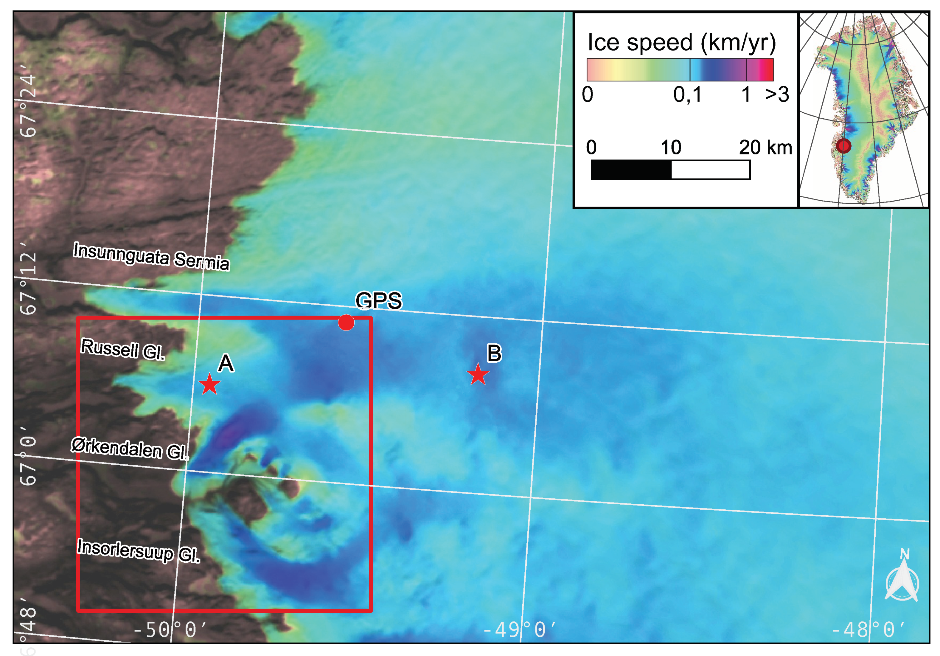
2.1. Study Area

We focus our analysis on a land-terminating sector located along the southwest coast of Greenland at a latitude of 67${}^{°}$N and longitude of 50${}^{°}$E. The sector ends in multiple ice tongues, named from north to south: Insunnguata Sermia, Russell Gletcher, Ørkendalen Gletscher, Insorlersuup Gletscher (Figure 1). This is one of the most studied regions of Greenland due to the relatively easy accessibility from the town of Kangerlussuaq.

The outlet glaciers in this region flow with speeds ranging from 100 to 250 m/yr during winter, while the surrounding regions display ice speeds around 50–60 m/yr in winter. Seasonal ice speed fluctuations have been observed in a number of studies in this region. They are commonly attributed to pressure changes in the subglacial drainage system [6,7,25,26,27,28]. When spring melt begins, ice speeds typically increase due to an influx of meltwater into the subglacial drainage system, which raises the subglacial water pressure and reduces the basal friction [25]. Ice speeds decrease later in the melt season (sometimes below its spring value) as the subglacial drainage system adapts with the establishment of efficient channels which accommodate the melt and so reduce water pressure at the bed. For the large area near the ice margin of the Russel sector, large accelerations from 100 to 250% above the winter mean, with the measured maximum of 360% in small isolated patches, have been reported [6].

2.2. Satellite-Derived Velocity Data

We use a combination of ice velocity measurements derived from satellite images collected between 2015 and 2019 by Landsat-8, Sentinel-1, and Sentinel-2. Landsat-8 (L8) is an American Earth observation satellite launched on 11 February 2013 by USGS and NASA as a continuation of the Landsat program started in 1972. The Operational Land Imager (OLI) on-board Landsat-8 acquires global moderate-resolution images (15 m for panchromatic channel or 30 m for spectral) in the visible and infrared parts of the spectrum with a revisit time of 16 days between 82.7${}^{°}$ north and south latitude. Images are provided as geocoded products by USGS, either in UTM or polar stereographic coordinates. Optical imaging requires solar illumination, and correspondingly there are a large number of acquisitions during austral and boreal summers and few in winter.

Sentinel-2a and 2b (S2) are twin optical observation satellites developed under the European Commission Copernicus Program launched into orbit in 2015 and 2017 respectively by the European Space Agency (ESA). They provide moderate-resolution multi-spectral images of Earth similar to that of Landsat-8. Images in 4 spectral bands (blue 490 nm, green 560 nm, red 670 nm, and near infrared 850 nm) are provided with 10 m resolution in UTM projection. Together the Sentinel-2 satellites have a revisit time of 5 days. Similar to L8, most of the acquisitions are made during the summer season when there is solar illumination.

Sentinel-1a was launched for the Copernicus Program by ESA on 3 April 2014, and was joined along the same orbit by Sentinel-1b on 25 April 2016. Sentinel-1 (S1) is a right-looking synthetic aperture radar (SAR) mission, observing with an incidence angle ranging from 29.1 to 46.0${}^{°}$. S1 is a C-band radar with a revisit time of 12 days per satellite and 6 days with the constellation. Acquisitions over land are made with the interferometric wide swath (IW) mode using progressive scans SAR (TOPS) technique. Using Gamma Software gamma-rs.ch, the bursts are de-ramped from their Doppler history and mosaicked together to form a single-look complex image with a ground resolution of 20 m in azimuth and 5 m in ground range [29]. Following the recommendations by PSTG, Sentinel-1 has acquired data continuously since June 2015 across a set of six tracks that cover the entire coast of Greenland, including the area of Russell Gletscher.

We use persistence surface features or speckle to track ice displacements between two images over the ice sheet [16,30,31] for optical data. We use the same methodology as presented in [19,23] to calculate a standardized cross-correlation between the reference image chip and the slave chips, which is based the Fortran code of ampcor [32]. For L8 [16], S2 [23], and S1 [18], sub-images of 32 × 32, 32 × 32, and 192 × 48 pixels are used respectively. The displacement maps in pixels are then converted to glacier surface velocity in meters per year and geocoded using the north polar stereographic projection. The final calibrated maps (see Figure 2) are resampled to a resolution of 150 m/pix; no spatial smoothing is applied at any of the steps for estimating speed. The x and y components of velocity in meters per year are stored independently as GeoTiff. We use the GDAL library gdal.org for all geographical transformations and formatting of the final files.

The estimated precision for the nominal cycle is about 50 m/yr, 40 m/yr, and around 20 m/yr for L8, S2, and S1 respectively, as reported by [19,21,23]. Shorter intervals are more sensitive to errors that are uncorrelated in time, such as those caused by the atmosphere or ionosphere, or errors from the correlation algorithm since surface displacement data are scaled by the observation interval used to derive velocity. The entire range of velocity errors in our data varies from about 50 m/yr (nominal L8 cycle) to 5 m/yr (24-days S1 cycle).

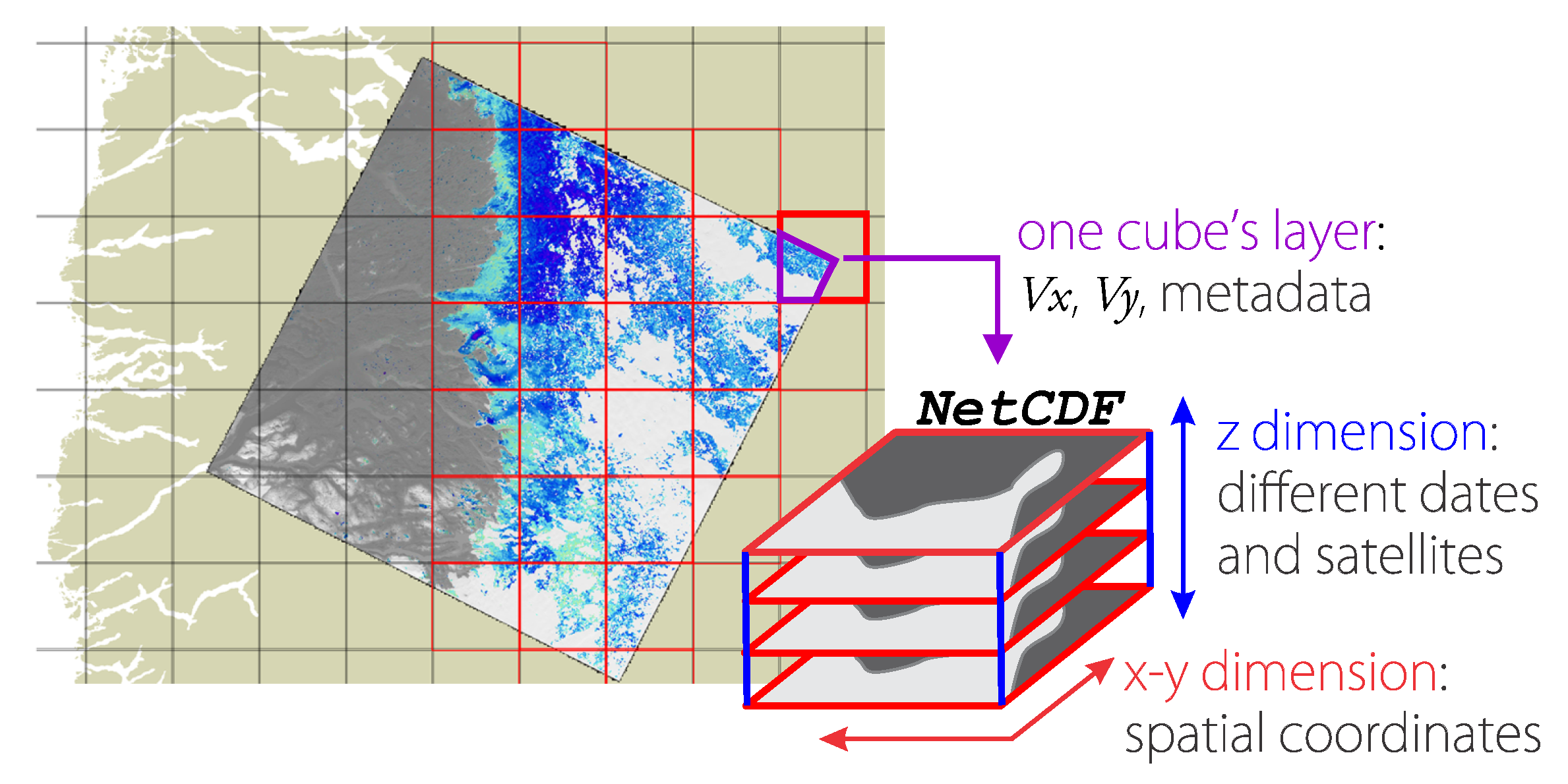
2.3. Ice Velocity Database Creation

To facilitate post-processing, our velocity maps are divided into areas of equal size of 37.5 × 37.5 km with a resolution of 150 m (thus 250 × 250 pixels). For each area, we extract and stack the velocity maps and associated metadata into “cubes” where the 3rd dimension z corresponds to the number of calculated speed maps (Figure 2). To avoid edge problems during post processing, the cubes overlap by 5 pixels (750 m). Each cube is a standardized dataset where all maps are stored on a common grid and the time series of the surface velocity can be easily extracted to calculate time-averaged maps or apply time-oriented post-processing. The cubes are stored in the GDAL-compatible netCDF format following the Climate and Forecast metadata conventions cfconventions.org. A cube file contains metadata about the cube itself (dimensions, corner coordinates, number of speed maps, etc.), surface velocity maps in meters per year in $x/y$ directions ($v_x$ and $v_y$ hereafter), associated errors, projection information, processing directory of source images, dates of master and slave images, repeat cycle, and sensor name.

${ϵ}_{v_x}$ and ${ϵ}_{v_y}$, which are the errors on $v_x$ and $v_y$ respectively, are independent in our processing chain. For the optical imagery with isotropic resolution, they are identical. However, in the case of Sentinel-1, we have a large difference between ${ϵ}_{v_x}$ (east-west) and ${ϵ}_{v_y}$ (north–south) components. This is due to the difference in pixel size between the azimuth and range and the fact that S1 tracks are more closely aligned with the north–south direction. The error on ice speed magnitude v is calculated as ${ϵ}_v=\sqrt{v_x^2{ϵ}_{v_x}^2+v_y^2{ϵ}_{v_y}^2}/v$.

We use speed measurements with time intervals shorter than 32 days (1 month) in order to capture rapid dynamic changes in ice flow, meaning that we use 16 and 32 day repeat cycles for L8, from 5 to 30 days for S2, and 6 to 24 days for S1. Longer time intervals would provide more precise velocity measurements but at the expense to temporal resolution, thereby limiting our ability to capture the seasonal velocity fluctuations we are interested in.

More than several hundred velocity maps per year can be obtained in our region of interest over the mentioned time spans, but the spatial coverage varies with sensor, location, and season: an example for year 2018 is given in Figure 3. The region above the equilibrium line about 30 km from ice margin has the poorest coverage because the surface is smooth and only a few surface features can be tracked with optical imagery. In this area, the S1 provides more measurements because the speckle tracking of SAR images does not require recognizable features on the glacier surface (e.g., crevasses) but is nevertheless limited by current acquisition plans that focus on marginal areas.

In summary, S1 is the main data source during the cold season (from November to April), particularly in the ice-sheet interior. However, its correlation drops significantly near the margin during the warm season when the glacier surface experiences melt. S2 and L8 optical sensors provide good correlation results along the ice margin where many surface features can be found, but perform poorly further inside the ice sheet where less features can be found, and provide no observations during the polar night (December-January) due to the absence of solar illumination.

Nevertheless, using the combination of all 3 sensors, we obtain a dense time series of ice surface velocity that allows us to investigate the seasonal ice flow dynamics. In Figure 4, we plot the time series for 2 different locations (point A and B, see Figure 1) with associated errors from January 2015 to September 2019 derived with 1308 (point A) and 908 (point B) individual velocity estimates by Sentinel-1, Landsat-8 and Sentinel-2. These time series are then used to evaluate the efficiency of different regression algorithms to create regularly sampled, filtered, and coherent time series of ice motion with reduced noise.

2.4. In-Situ GPS Measurements

We compare our satellite-derived speed measurements with GPS in-situ data made in one location between 15 July 2014 and 14 July 2017 collected as part of an ice dynamics study [33]. When first set up in July 2014, the GPS was located at the position 49.567${}^{°}$W and 67.182${}^{°}$N and moved by about 371 m over the course of the 3 years. GPS position was measured every 15 s, except when the system ran out of power during the winters. From the registered GPS locations we compute mean daily displacements (Figure 5), and then average them over 3 weeks to be comparable with our dataset (see Section 5.4 and Figure 8).

3. Velocity Post-Processing/Data Reduction

The velocity dataset from multiple sensors contain a large number of incorrect or noisy displacements superimposed on the real variability of the ice flow. Despite the noise, sub-seasonal fluctuations in speed are clearly captured by Landsat and Sentinel satellites (see Figure 4 and Figure 5). Here, we take advantage of dense data series and try several types of post-processing with the final goal of producing a filtered, continuous, and coherent time series of velocity with reduced noise compared to the individual measurements.

As detailed previously, we have generated ice speed data cubes from S1, S2, and L8 data, where every measurement is stored on a common spatial grid and the 3rd dimension corresponds to the discrete irregular time interval of the measurements. Thus, each pixel contains a velocity time series. For each time series, we independently apply and compare three different approaches of data smoothing and noise reduction: statistical rolling mean and median, cubic spline regression, and linear non-parametric local regression to obtain continuous filtered time series. The date of each measurement is assigned as the center between the first and second satellite images dates in the velocity estimation pair. Thus, we do not take into account the disparity of time spans of derived velocity (from 5 to 32 days). The regressions are performed on $v_x$ and $v_y$ separately, but implementation of regressions on the velocity magnitude v and direction a are discussed as well (see Section 5.2). We describe three data reduction approaches in detail in the following sections.

3.1. Rolling Mean or Median

Rolling mean, also called moving average, is the most simple statistical approach used to analyze series of ordered data. We use a weighted mean with the weights defined for each measurement individually as $1/{ϵ}^2$, where $ϵ$ is the error associated with a source velocity map. The increased size of the data subset used for the mean decreases the final error at the expense of the temporal resolution. Different subset sizes were tested from 1 to 4 weeks (see Section 4.1 and Section 4.2, Figures 8 and 9a,b) to assess which subset sizes is best suited for our datasets.

Ice velocity sampling is not uniform in time (as explained in Section 2.3). There are periods with fewer measurements, which was the case before 2016, but more recent years have had more frequent sampling. Moving average generally implies that the time-series is continuous and evenly spaced in time, which is not the case for our time series. We note that having measurements that are not uniformly spaced across a subset window can introduce a bias in the final average.

From a statistical point of view, the moving average, when used to filter a time series, is likely to be biased by anomalies (outliers). A more robust estimate would be the rolling median with the disadvantage of not being able to use different weights depending on the measurement errors. We also tested the rolling median method and obtained the results that are very similar to the weighted rolling mean. Thus, only the rolling mean results are used in our analysis.

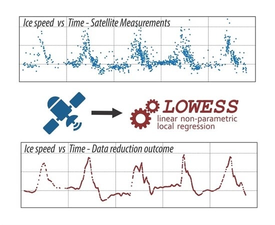
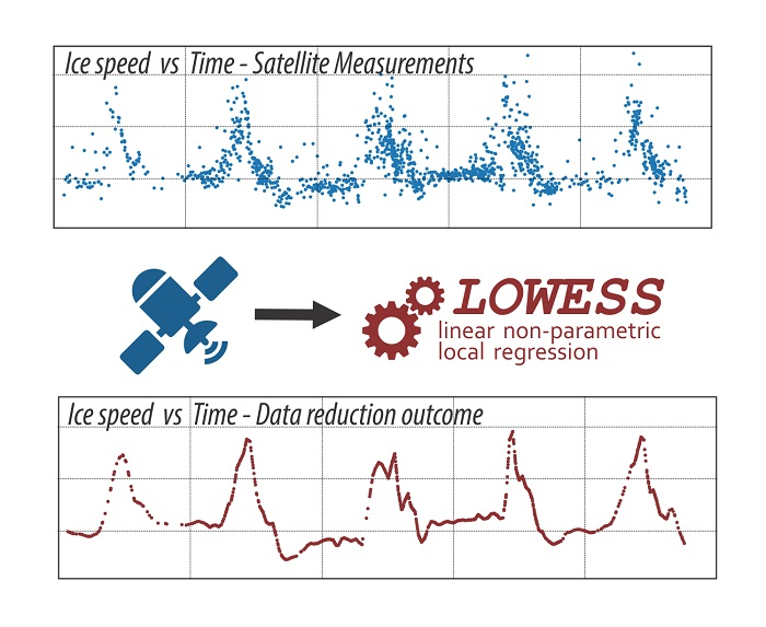
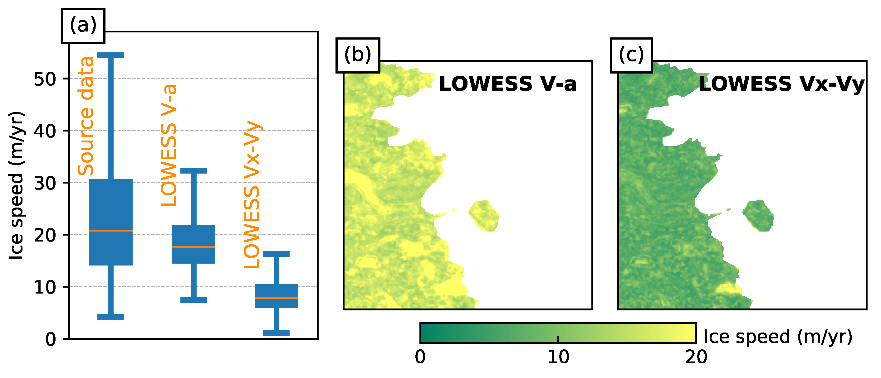
3.2. Linear Non-Parametric Local Regression: LOWESS

Locally weighted scatterplot smoothing (LOWESS) is a moving non-parametric regression that fits a regression model on the k closest samples. Local regression is a statistical method for robustly fitting smoothing curves without prior assumptions about the shape or form of the curve. This algorithm, which was specially designed for noisy and scattered datasets, was introduced by W.S. Cleveland in [34], and was further developed in [35]. It is now used for a wide range of applications, including the noise reduction in satellite derived measurements, most commonly for studies of seasonally evolving vegetation [36,37,38]. The basic principle of the method is to the fit the data points (independent variables) using a linear or quadratic function in a moving fashion analogous to that used for a moving average applied to a time series. The mathematical concept is illustrated in Figure 6. As shown in the sub-panel of Figure 6, a regression is performed using a low-order polynomial function on a localized subset of data centered around a particular point in the data series. The k closest neighboring points participate in the regression estimation with specific weights. The weighting is based on the idea that close points are more likely to be linked together in a simple way than distant points. Following this principle, greater weight is given to the points that are close to the local value. The procedure can be repeated several times; new weights are estimated, allowing one to remove outliers from the final solution, as illustrated with the green point in Figure 6. Depending on correspondence between data density and the subset size, some potentially correct measurements could be interpreted as outliers and ignored in the final solution, as with the orange point in Figure 6). These local regressions can be performed at any specified locations or for each input point. The final curve is the merge of all local regressions.

Here, we use the algorithms from Scipy has2k1.github.io/scikit-misc/ and Statmodels statsmodels.org adapted in Python by P. Gerard-Marchant. The first can provide additional statistics that are useful for experimental testing; however, the second seems to perform better for intense computation, and is therefore more useful given the large number of regressions performed in our analysis.

There are four key parameters that can be defined in the LOWESS algorithm. The fraction f, that is comprised between 0 and 1, defines the amount of smoothing and corresponds to the fraction of the time-series that is used for each local regression. Thus, large value of f will use more data points for each local estimation and provide a smoother solution, while a small value will reduce the number of data points used and so allows the regression to be closer to the initial data.

The weights w applied to measurements at each regression can also be specified. In the original paper [34] the author defines the optimal choice is a bell-shaped cubic function that gives maximum weight to the closest points and diminishes quickly to zero with the distance from the evaluated point (as the gray-colored area represents on the sub-panel at Figure 6). This is an option by default for Python LOWESS implementations. Additionally, user-defined weights can be introduced into the skmisc.loess code, and in our analysis are based on the source data errors. Similarly to the rolling mean, we tested a case of weights defined as $1/{ϵ}^2$, where $ϵ$ is the error associated with each data point. We obtain a negligible change of fitted values with no clear improvement, indicating that the default weighting system is sufficient to obtain robust regressions. Thus, these additional weights are not used in our further tests.

To address data anomalies, several iterations of LOWESS can be applied to re-estimate neighbors’ weights to identify and eliminate outliers. While the initial weights of a local fit rely only on x-axis distance to the neighbors, during the LOWESS iterations, data subsets with the largest deviation range are excluded to find a state with minimal root-mean-square deviation.

Linear and quadratic local regressions cover most cases [34] and the polynomial order of the local regression can be set to 0, 1, or 2. Using a zero degree polynomial turns LOWESS into a weighted moving average.

In our processing, we use a linear function, as the quadratic regression tends to be less robust against noisy datasets. We use 3 iterations to obtain the most robust results [34]. Weights are defined by the default cubic function as given in [34], and no additional error-based adjustment of weights is applied. The best choice of the smoothing parameter f depends on our initial data and is discussed on the following section (see Section 4.1 and Section 4.2, Figures 8 and 9c,d).

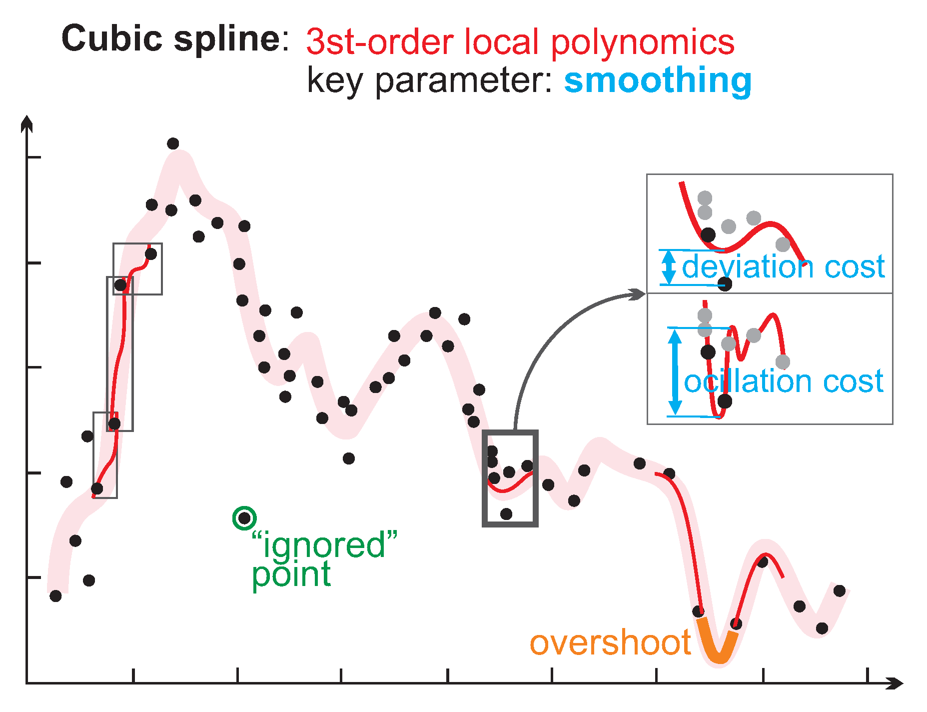
3.3. Cubic Spline Regression

A cubic spline is a piecewise function that interpolates a set of data points with third-degree polynomic between neighbors in the way to guarantees smoothness of fitted curve and closeness to the source data points [39]. Its mathematical principles are illustrated in Figure 7. The “piecewise” function means that it fits data subsets as in the rolling mean and LOWESS, and thus is not a global fitting function. For each data subset that contains two neighboring points a cubic function is fitted with a constraint to satisfy the continuity of the global solution and its first and second derivatives. Here, we use a cubic smoothing spline designed specifically for noisy observations. Contrary to interpolation cubic splines, cubic smoothing splines have additional functional constraints: (i) to minimize the squared error between the dataset and spline, and (ii) to minimize the curvature. These two constraints are controlled by the smoothing parameter f, which varies from 0 to 1. When $f=0$, the spline regression performs infinite smoothing, which corresponds to a linear least-squares fit on the entire dataset. When $f=1$, the curve is the natural cubic spline that passes through all initial points.

When an outlier is located in a zone well-populated by “true” points, it can be successfully ignored by the spline regression (green point in the Figure 7). However, when a portion of the time series is less frequently sampled, the cubic spline is less constrained and can create unrealistic overshoots (orange part of the line in Figure 7).

We use the cubic spline approximation with a customizable smoothing parameter and weights from CSAPS github.com/espdev/csaps, which is based on [40]. Weights are provided in the same way as for the rolling mean ($1/{ϵ}^2$, where $ϵ$ is the error attributed to speed measurements). The best parameter of f will depend on data density and distribution of outliers, and could therefore change between regions. In the following sections, we discuss this choice of f that provides the best regression on our time series (see Section 4.1 and Section 4.2, Figures 8 and 9e,f).

4. Results

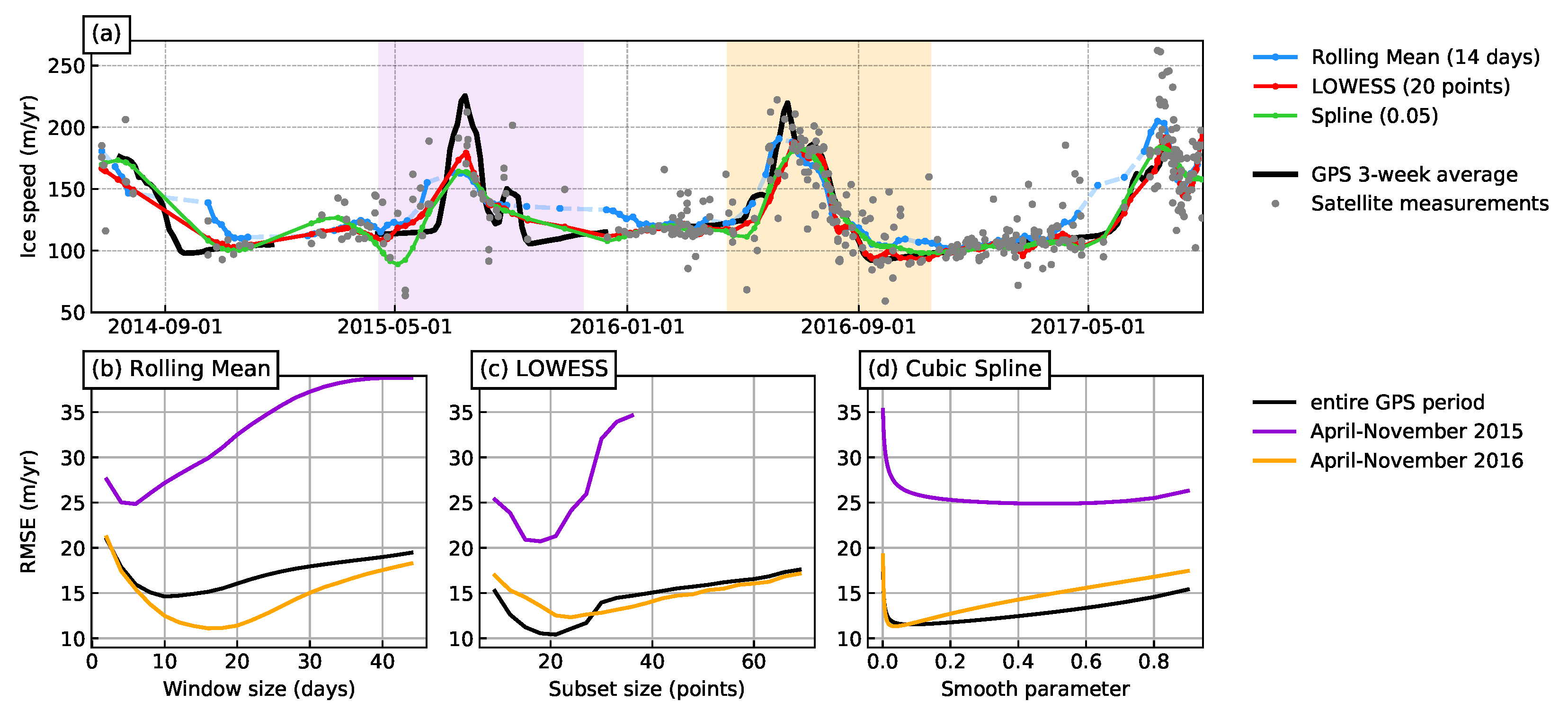
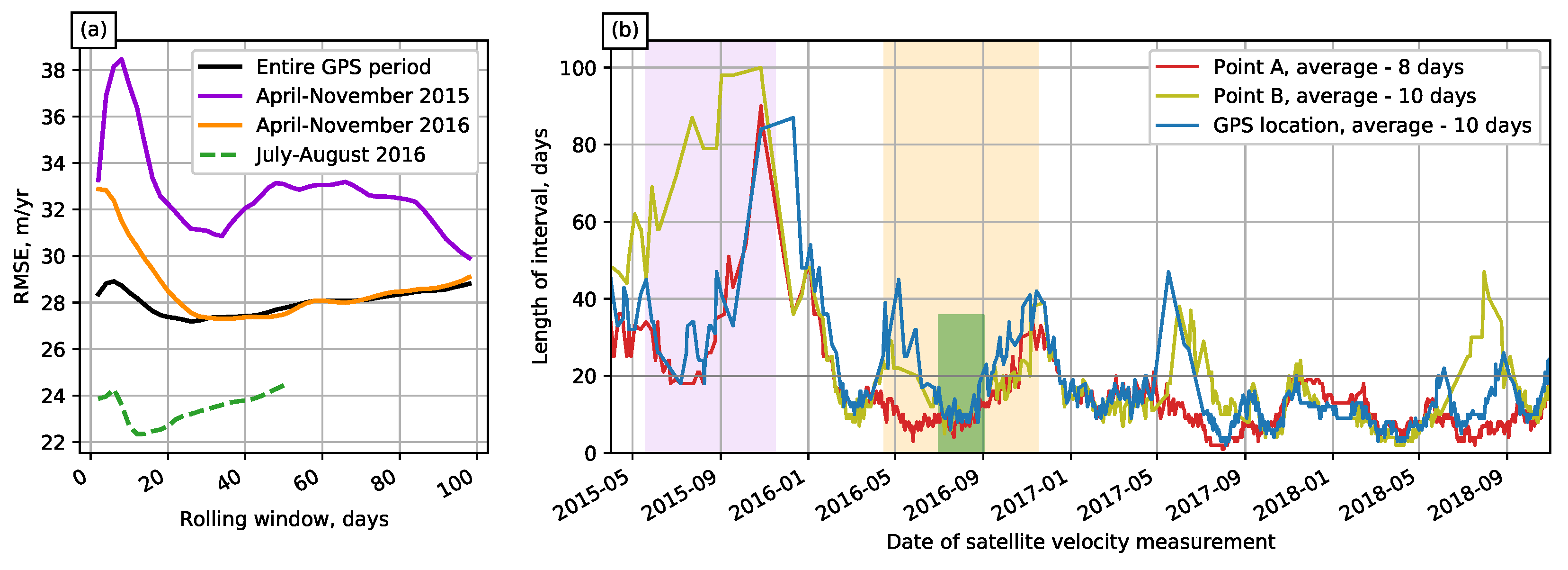
4.1. Comparison with GPS-Based Measurements

We first compare our initial and reduced ice speed time series with the 3-week moving average of ice speeds derived from GPS (Figure 8a). Over this averaging interval, the GPS best matches the satellite-derived data. (see Section 5.4 and Figure 12a). GPS ice speed is used as ground-truth since the velocity errors are less than 1 m/yr, while errors from satellite measurements are at best 7 m/yr and usually around 30 m/yr. The comparison is done by computing the root-mean-square error (RMSE) against the GPS for the individual measurements and then testing the sensitivity of different regression methods to parameter changes.

We found that the RMSE of S1, S2, and L8 combined measurements versus 3-week moving average on GPS time series is about 27 m/yr when the entire time period is considered (see Figure 12a). For the data reduction methods, the minimum RMSE values (15, 12, and 10 m/yr) are found when the chosen adjustment parameters for the rolling mean, the cubic spline, and the LOWESS regressions, are a window size of 12 days, a smoothing parameter of 0.05, and a subset of 20 points, respectively (Figure 8b–d). We note that: (i) the RMSE is improved by the regressions compared to the original measurements, and (ii) LOWESS provides the best RMSE compared to the rolling mean and cubic spline.

We also tested two shorter periods, one from 15 April 2015 to 15 November 2015 and another from 15 April 2016 to 15 November 2016 (violet and orange colors respectively in Figure 8). These periods are both characterized by important speed fluctuations (while speeds are almost constant during winter) but differ by the number of acquisitions made, with only 38 for the first and more than 102 for the other. For the second period (2016), the RMSE is improved by a factor of two compared the first period. This shows the improvements gained by increasing the number of acquisitions in order to more precisely capture the seasonal variability. We also found that when the number of observations is low and they are not equally distributed through the time LOWESS performs better than the rolling mean and the cubic spline regression.

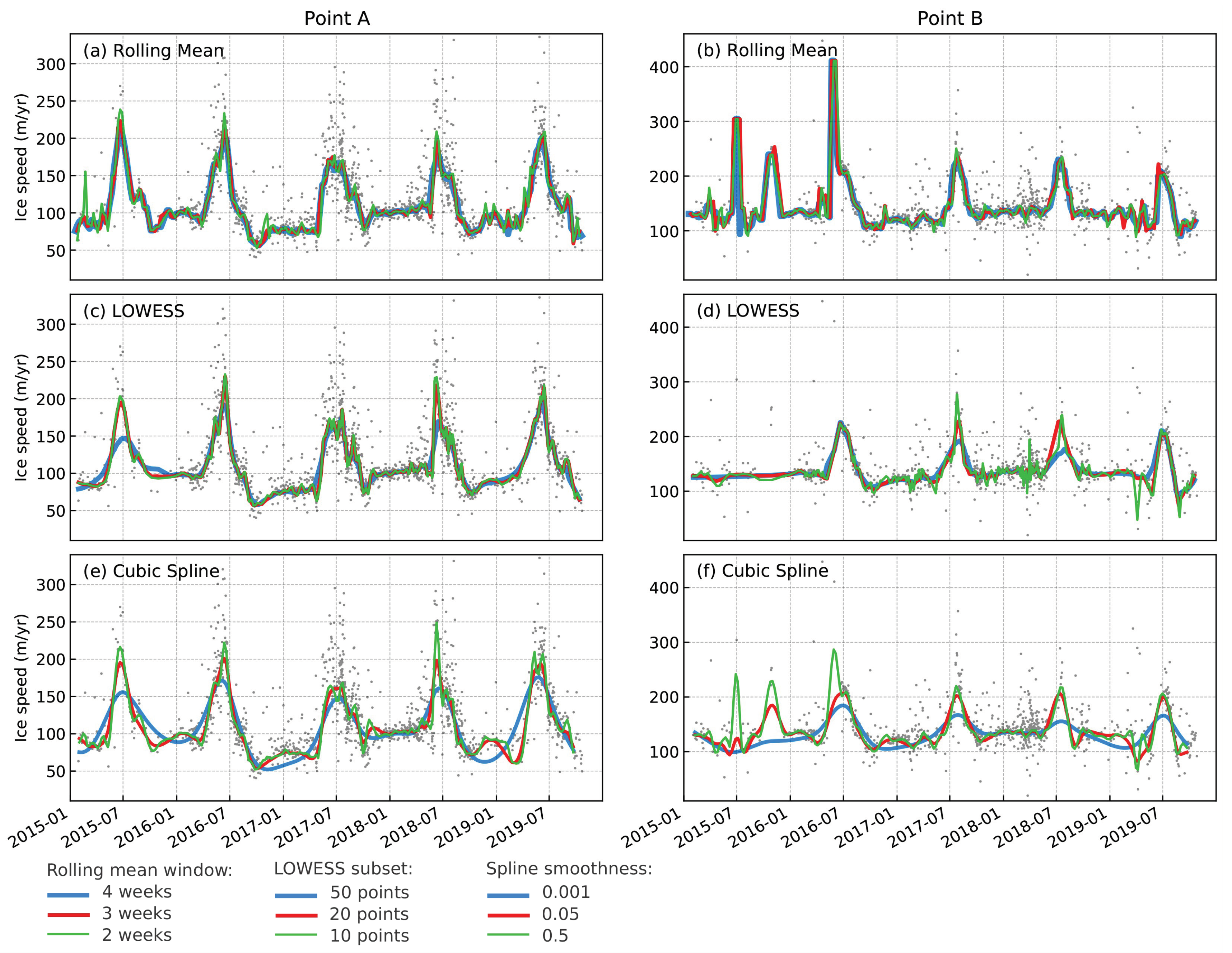
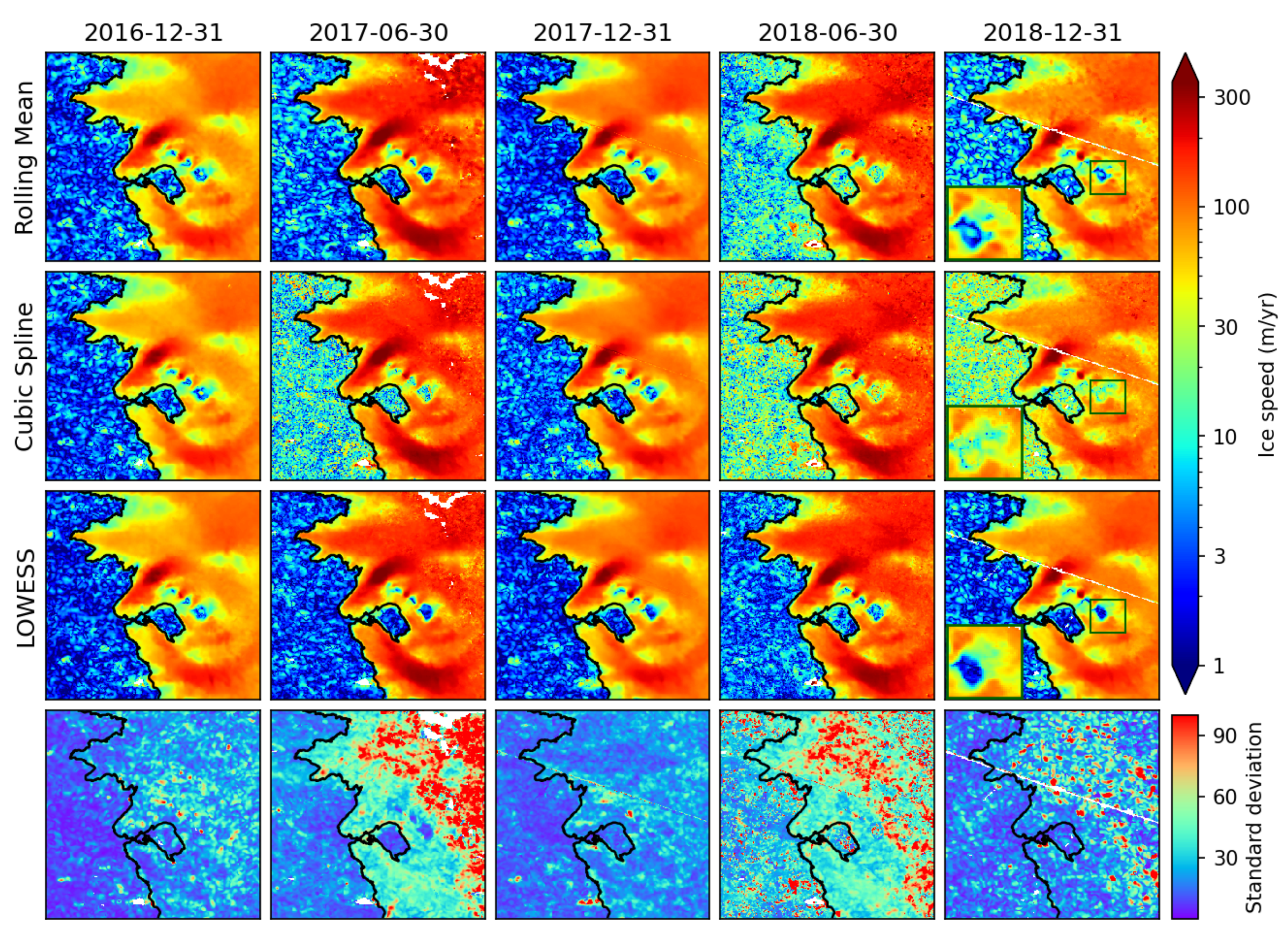
4.2. Time Series Post-Processing

Figure 9 presents the results using the different reduction methods on our time series for two locations (point A and point B) as shown at Figure 1. Point A (67.099${}^{°}$N, 49.953${}^{°}$W) is located relatively close to the ice-sheet margin in an area of relatively fast flow. This area experiences strong summer acceleration (see Figure 4). Winter speed from October to May is around 100 m/yr, with a minimum in October that increases slowly until May. In general, summer speed-ups start gradually in May and end in mid-July, and the maximum speed is about 170–200% faster than winter speeds, which equates to 270–300 m/yr. During the summer season, many surface features are present, allowing the correlation using optical sensors to work well, resulting in a dense velocity time-series. However, only S1 provides observations during winter.

Point B (67.134${}^{°}$N, 49.177${}^{°}$W) is located about 40 km from the ice margin in a flat smooth area with less surface features. This impacts the ability of the optical sensors to capture ice displacement during all seasons. Nevertheless, we found that, at this location, winter speed is around 120 m/yr and ice flow increases by about 70 to 90% during the summer season. The evaluation is more challenging than for point A because of fewer successful measurements during the melt season; however, it seems that the maximum ice speed is reached around mid-July which is later than for point A (mid-June).

Figure 9a,b presents the results of the weighted rolling mean using averaging windows of 2, 3, and 4 weeks. The rolling mean provides relatively good regression when the frequency of measurements is high. It is however impacted by outliers, which is especially true for point B where the speed magnitude sometimes jumps by hundreds of meters per year for periods with sparse and noisy measurements. As expected, by increasing the size of subsets used for averaging, we obtain a more robust results at the expense of temporal resolution. Given the data noise and time interval between master and slave images (5 to 30 days), a realistic balance between robustness of the regression and time resolution seems to be 3 weeks for dense time-series (as in location A), similar to the comparison made against GPS. However, we note that for sporadic time-series, even a window of 1 month is sensitive to outliers, as seen during July 2015 or 2016 for point B.

Figure 9c,d show the result for the LOWESS regression using various fraction parameters, corresponding to subsets used for the regression with 10, 20, and 50 points. Using the largest subset size (50 points) provides a smooth result at the expense of temporal resolution, while the smallest subset size (10 points) is less constrained and is sensitive to data noise. As expected, 50 point subsets tend to underestimate the amplitude of the summer speed-up the most. Therefore, the best comprise seems to be a fraction parameter using 20 points.

Figure 9e,f presents the cubic spline regressions for different smoothing parameters. Using a large value ($f=0.5$, e.g., less smoothing) helps to capture the rapid accelerations during the summers, as seen for point A (Figure 9e). However, it also generates deep and unrealistic velocity deviations (overshoots) when few measurements are available as for point B (Figure 9f). On the contrary, using a low value ($f=0.001$, strong smoothing) tends to provide a robust regression that is not impacted by the outliers but comes at the expense of temporal resolution and capturing the amplitude of the speed variations. An intermediate smoothing value around $f=0.05$ seems to provide the best compromise between resolution and outlier impact for both locations.

The data reduction using statistical and regression methods provides ice velocity in a corrected, ordered and simplified form. All tested methods using the fit with their optimized parameters more or less capture the seasonal velocity variations. Their solutions are very close when the source data are well populated, evenly distributed over time and contain few outliers as for point A (Figure 9). However, differences appear when times-series are less populated, like for point B (Figure 9). At this location where fewer and often noisy measurements are obtained, the simple statistical regression using rolling mean is much more sensitive to outliers, while more complex regressions such as spline and LOWESS still provide robust reconstructions. Point B is representative of results obtained in the ice-sheet interior.

Cubic spline seems less appropriate than LOWESS, especially in case of sporadic and noisy data. Indeed, we observe clear overshoot effects on the cubic spline solutions when the number of measurements is limited, such as during February 2019 for point A or before January 2016 for point B (Figure 9), whereas LOWESS converges to a more realistic solution. This is also confirmed by the comparison with the GPS ice speeds, where the best RMSE is obtained by the LOWESS algorithm (Figure 8).

In Figure 10, we present the results in June and December of years 2016, 2017, and 2018 using the best adjustment parameters found previously for a complete data cube shaped as described in Section 2.3. The cube consists of 250 × 250 pixels corresponding to an area of 37.5 × 37.5 km (red square in Figure 1); thus, there are 62,500 regressions done for each approach. The black line corresponding to the ice margins delimits the boundary between ice-free (to the left) and ice-covered (to the right) area. As described previously, adjustment parameters are a 3-week window for the rolling mean, 0.05 smoothing for the cubic spline, and 20 points for the LOWESS. The standard deviation of the source measurements is calculated over 2 weeks. Although no spatial filtering or smoothing is applied, the results of each individual regression in a pixel are very consistent with their neighboring pixels, providing spatially more homogeneous results than original data. All methods capture the seasonal speed fluctuations; however, LOWESS provides the most robust and smooth solution with less visible noise and speeds closer to zero over the ice-free areas. This result is also highlighted in the sub-panels showing a zoom where ice is flowing around a nunatak. Here, LOWESS is the only method with speed close to zero over the entire rock surface (less than 3 m/yr in average), while the rolling mean and the cubic spline are much noisier and ice speeds approach 20 m/yr.

5. Discussion

Since 2014, Landsat-8, Sentinel-2, and Sentinel-1 have acquired large amounts of data over Greenland. We have processed these spaceborne observations and generated maps of ice motion. Having seamless maps of ice velocity is crucial for the scientific community to study glacier dynamics and the evolution of ice sheets in a warmer climate. However, generating sub-seasonal velocity times series over large spatial scales is technically challenging using data from medium resolution sensors where the individual measurements can remain noisy.

Here, we show that (1) combining Landsat-8, Sentinel-2, and Sentinel-1 provides continuous estimate of ice velocity that one sensor alone would not; (2) using statistical or regression data reduction methods can help reducing the individual noisy measurements into filtered, ordered maps; (3) with LOWESS regression we are able to produce the reconstructions that agree well with ground-truth measurements from GPS even in slowly moving areas.

5.1. Multi-Sensor Time Series

The main reason why we rely on different sensors to obtain continuous times series is that each sensor contributes uniquely to the time series. The integration of S2 and L8 optical sensors and the SAR S1 provides continuous measurements through the entire year, as shown in Figure 4. Correlation drops significantly for Sentinel-1 due to surface melt during the summer months near the margin, but the use of S2 and L8 can over come this issue. Conversely, during the winter months, optical sensors are unable to observe due to the polar night and very smooth surface, yet S1 provides reliable observations. While optical sensors S2 and L8 replace S1 during summer month along the margin, we note that it remains challenging to capture the seasonal changes for the upper part of the glacier where fluctuations in speed are small compared the intrinsic errors of the tracking techniques. This is especially the case during the first part of summer season due to the limited number of S1 acquisitions in the ice-sheet interior and also because optical S2 and L8 fail to find surface features used for tracking (Figure 4, point B).

Comparing our time series to published results [1,6,26,27,28], we found the same range of values, spatial distribution, and general seasonal behavior of seasonal velocities. In general, summer speed-ups start gradually in May and ends in mid-July with acceleration up to 200% compared to winter speeds. The main differences come from the number of ice speed maps produced, where the number of ice speed maps generated by most studies is between 10 to 20 maps per year [1,6,26,27]. For example, the GoLIVE project nsidc.org/data/golive can at most provide 22 velocity maps using only Landsat-8 with a 16-day repeat cycle. We found the only study with high enough data density to capture seasonal fluctuations well is [28], which generated 96 velocity maps from Sentinel-1 between January 2016 and December 2017.

To summarize, the combined observations from Landsat-8, Sentinel-1, and Sentinel-2 produce surface velocity time series in the Russel sector with sub-seasonal resolution for the entire marginal area (about 50 km from the ice margin). Thus, making velocity time series derived from spaceborne data is not only possible for fast outlet glaciers, but also for slow areas such as the land-terminating sectors flowing at speeds of 70 m/yr. However, the number of observations, the accuracy, and the correlation success rate are lower farther inland, which still limits our ability to properly capture the more subtle seasonal signals. For these regions, additional SAR acquisitions would be an asset that could fill this data gap because they do not depend directly on surface features for correlation, as is the case for optical sensors. We therefore recommend extending the 6-day S1 repeat coverage of the Greenland coast to the entire Greenland ice sheet.

5.2. Which Variables to Fit?

Before we discuss the different approaches used to reduce our measurements, we would like to compare two different ways of using speed measurements. The satellite-derived ice velocity is defined by the movement in x and y-direction independently ($v_x$ and $v_y$) and our regressions is performed on these components. However, another strategy could be considered by using the speed magnitude v and flow direction $\alpha$, where $v_x=vcos\left(\alpha \right)$ and $v_y=vsin\left(\alpha \right)$. We test both approaches in an ice free area where “ice speed” should be equal to zero. Deviations from zero in our observations comes from the random errors in the tracking algorithm and such non-moving regions can be used to evaluate the final precision of our measurements [19,23]. Here, we calculate the distribution of v from the original measurements as well as from the solutions given by LOWESS when used to adjust either ($v_x$, $v_y$) or (v, $\alpha$). We found that the averaged values for v are 21 ± 19 m/yr from the original mixed satellite-derived measurements. After applying the LOWESS regression on the components $v_x$ and $v_y$, we obtain an average value for v of 8 ± 4 m/yr, while being 17 ± 6 m/yr when using the direction $\alpha$ and magnitude v (Figure 11a).

It appears that fitting $v_x,v_y$ gives a better solution by a factor of 2 with absolute speed v closer to 0, compared to fitting v and $\alpha$. The difference between the solutions can be explained mathematically. Since $v_x$, $v_y\in \mathbb{R}$, when the ice speed approaches 0, $v_x,v_y$ components with their associated errors are distributed around zero with positive or negative values, and thus averaging multiple independent measurements of $v_x$ and $v_y$ tend towards zero. While, as $v\in {\mathbb{R}}_{+}$ and errors can be only positive, the same averaging but on the velocity magnitude v tends toward the measurement error instead of zero. If absolute glacier speed is much higher than the intrinsic error of the measurement, then this is not an issue, as the distribution of v will not be truncated. However, when analyzing changes for areas flowing at a speed comparable to the measurement errors, one should use $(v_x,v_y)$ rather than $(v,\alpha )$.

5.3. Data Reduction for Ice Velocity

Methodologies applied on the ice velocity time series to reduce data to a corrected, ordered, and simplified form have been very simple, and currently rely on statistical averaging on a monthly to annual basis [19,21,23,28] or using spatial filtering to remove outliers without any time context [4,41]. This partly comes from the limited number of available measurements or the use of more accurate sensors in previous studies (e.g., TerraSAR-X or TanDEM-X) [1,3]. As observations from medium resolution sensors (Landsat-8, Sentinel-1, or Sentinel-2) become routinely available, the need for more advanced methodologies is important and the results presented here are of interest to the glaciological community.

From the three different methods we tested (Figure 8, Figure 9 and Figure 10), we found that a moving average (rolling mean or median) can be used only when the sampling of the time series is dense enough and homogeneous so that the mean can be computed on enough measurements to obtain statistically robust estimates (Figure 9a,b). That is usually the case for the ice-sheet margin but it is less true farther inland. Methods using local polynomial or spline regressions are more robust than the simple statistical rolling mean. In our case, the non-parametric local regressions (spline and LOWESS) seem to be more adapted to reduce velocity time-series noise than global regression function that would require a specific mathematical description of the speed fluctuations. In other words, the flexibility of local regressions is able to describe a complex and highly non-linear processes for which no trivial mathematical models exist yet. However, we still observe differences between the regression approaches. Cubic spline regression has the tendency to provide inadequate solutions when poorly constrained, where LOWESS seems more robust. As for the moving average, when a piece of the time series is less populated by data, the solution of the cubic spline regression “overshoots.” LOWESS does not have that limitation as the local regressions are based on the k nearest data points and thus the data subsets will adapt their time lengths.

Although LOWESS is a more robust tool, it comes at the cost of a longer computing time. LOWESS processing takes about 2 h on one CPU (Intel Core i5 2.30 GHz) for a cube of 250 × 250 pixels containing 1500 speed maps. This is 10 times longer than the computation of the moving average, or 5+five times longer than the cubic spline regression. Its large-scale application would therefore require further optimization of the code and/or the use of parallel computing. Thus, we support the use of rolling mean or cubic spline regression as a faster solution when measurements are frequent, accurate, and equally distributed in time, while we opt for LOWESS otherwise.

5.4. Temporal Resolution and Measurement Accuracy

It is important to evaluate at which temporal resolution the original and final reduced time series can represent the temporal variability of the ice flow. Here, we have mixed observations with repeated cycles of up to 32 days, making it difficult to assess at what typical temporal resolution our initial and fitted time series capture the fluctuations in ice velocity. For the combination of S1, S2, and L8 sensors, the temporal resolution is restricted by their own precision and the repeat cycles related to the observation frequency. According to estimations [19,21,23], every sensor can track ice displacement of roughly one-tenth (optical) or one-fiftieth (SAR) of a pixel with a temporal resolution corresponding to its shorter repeat cycle. This would correspond to ice speed changes of about 70, 35, and 30 m/yr over 5 days, 16 days, and 6 days for S2, L8, and S1, respectively. Such range is enough for the fastest glaciers of Greenland [1,21] but is a limiting factor for slower glaciers, such as the Russell sector. Therefore, when using the large number of acquisitions made by these sensors, we need to find the right balance in our regression approaches between (i) improving the speed estimation accuracy by increasing the size of the subset used to fit ice velocity at a specific date, and (ii) degrading the temporal resolution.

To evaluate the temporal resolution of the original satellite-derived time series, we average the GPS-based ice speed using different windows and calculate the root-mean-square deviation between the GPS and our space-based measurements (Figure 12a). We found the best agreement when GPS is smoothed with a window of 3 to 4 weeks (solid lines in Figure 12a), with a RMSE about 27 m/yr.

The GPS point is located more than 20 km from the ice margin. Closer to margin, more data are available and we can expect that the temporal resolution of our time-series would be slightly better. To prove this idea, we focus on a short period between July and August 2016 (dashed green line in Figure 12a), when the density of measurements in the GPS location is almost the same as for point A (Figure 12b). We found that the estimated temporal resolution is about 2 weeks when a dense time series is available with RMSE dropped to 22 m/yr.

As the LOWESS regression does not use a fixed window but the k nearest data point, the temporal resolution of regression solution will therefore vary depending on the rate of sampling of the input data. Previously, we evaluated that a subset of 20 measurements corresponds to the best adjustment parameter for LOWESS (Section 4.1). After 2015 (when Sentinel-2 and Sentinel-1b were introduced), an interval of 2–3 weeks always contained more than 20 measurements. In Figure 12b, we also evaluated the size of the weighted part of LOWESS subsets (weight > 0.5) for the regressions, which gives a good idea of the temporal resolution we can expect after the regression. Since 2016, the duration of the subsets used by LOWESS is always less than 40 days but often shorter than 20 days. This value is comparable to the repeat cycles (up to 32 days) used here; therefore, we can expect that the temporal resolution of final reduced time-series is not degraded compared to the initial measurements by the LOWESS algorithm.

The comparison with the GPS also allows us to investigate the accuracy of our time-series. Speed estimations from images obtained by S1, S2, and L8 when combined have a RMSE of about 27 m/yr. After using the different regression approaches, the RMSE is improved by a factor 2 to 3: the best reconstruction is obtained by LOWESS with a RMSE of 10 m/yr. We note that this evaluation is performed at only one single location about 30 km inland from the ice margin and limited to the period from 2014 to 2017 when the GPS was installed. We think that the comparison would be better nearer to the ice margin where correlation success increases, yet lower further inland.

To summarize, it appears that using regression approaches on dense time-series improves significantly the precision of the ice speed maps without degrading the temporal resolution compared to the individual measurements.

5.5. Other Potential Ways of Improving Post-Processing

In our study, the algorithms applied to the data only use the temporal dimension independently between each point in space. It would be possible to take into account the physical spatial cohesion of the glacier and thus use the information contained in adjacent locations to locally improve the reconstruction of ice velocities (e.g., do spatial filtering or smoothing, fill gaps, or discriminate short speed-ups from outliers). Introducing adaptive parametrization depending on the number of measurements could improve the results as well, especially for capturing the sharp peak at the beginning of the summer speed-up. However, the significant increase in computational cost to test find the solution would need to be addressed. Here, we have treated the diverse revisit times indifferently (5 to 32 days, except for the error/weight estimation); advanced algorithms could more carefully use this information to obtain more precise reconstruction of the ice speed, as shown by [24,42].

We also could envision an application of “time-memory” techniques to our time-series, meaning that we could eventually take advantage of the seasonality of the ice motion fluctuations to improve locally in space and time our reconstruction. This would required long time memory to be properly used. Non-classical machine learning techniques such as ensembles or neural networks are now broadly proposed as time-memory methods (e.g., [43,44,45], but the questions regarding reproducibility or accurate learning should be treated carefully given the relatively short period with dense measurements we have obtained so far and the variability of velocity fluctuations from year to year. Finally, one of the obvious advantages of our simple approaches is the robust reproducibility, meaning that such data reduction methodology could be applied on a much larger scale.

Another way to improve the final quality could be to directly refine the matching algorithm that derives the ice motion. For example, using reverse correlation [46,47], triangle closure [22], or more than two observations would prevent false correlation and improve single measurement accuracy. However, in all these cases, the obtained precision would be still limited by the resolution of the sensor and the distance moved by the glacier in a given period of time. Therefore, post-processing of the large spatio-temporal dataset would still be needed to improve the precision and temporal resolution to obtain corrected, ordered, and simplified reconstruction of the ice dynamics.

6. Conclusions

In this study we derived ice velocity from three different sensors over the sector of Russell Gletscher, Southwest Greenland, using data acquired between 2015 and 2019 by Landsat-8, Sentinel-2, and Sentinel-1, which all have repeat cycles of shorter than 32 days. These large datasets provide frequent estimation of the ice dynamics but are relatively noisy for the regions of ice flow where speeds are slower than a few hundreds of meters per year. We therefore investigated three different methodologies to post-process the ensemble of available data with a goal of reducing the initial measurements to a filtered, ordered, simplified form. We found that using linear non-parametric local regression (LOWESS) provides the best result compared to rolling mean and cubic spline regression in terms of robustness against data availability and precision of the reconstruction. For the slowly flowing land-terminating areas, such as the Russell sector, the processing results offer robust reconstruction at a temporal resolution between 2 and 3 weeks with a mean accuracy of about 10 m/yr on the annual time scale. As new observations become even more routinely available, post-processing analysis will become instrumental to providing reduced reanalysis of ice dynamics. In this context, the presented methodology could be applied to the entire Greenland ice sheet with an aim of reconstructing comprehensive sub-seasonal ice flow dynamics and mass balance.

References

- Moon, T.; Joughin, I.; Smith, B.; Van Den Broeke, M.R.; Van De Berg, W.J.; Noël, B.; Usher, M. Distinct patterns of seasonal Greenland glacier velocity. Geophys. Res. Lett. 2014, 41, 7209–7216. [Google Scholar] [CrossRef] [PubMed] [Green Version]
- Armstrong, W.H.; Anderson, R.S.; Fahnestock, M.A. Spatial Patterns of Summer Speedup on South Central Alaska Glaciers. Geophys. Res. Lett. 2017, 44, 9379–9388. [Google Scholar] [CrossRef]
- Moon, T.; Joughin, I.; Smith, B. Seasonal to multiyear variability of glacier surface velocity, terminus position, and sea ice/ice mélange in northwest Greenland. J. Geophys. Res. Earth Surf. 2015, 120, 818–833. [Google Scholar] [CrossRef]
- Lemos, A.; Shepherd, A.; McMillan, M.; Hogg, A.E.; Hatton, E.; Joughin, I. Ice velocity of Jakobshavn Isbræ, Petermann Glacier, Nioghalvfjerdsfjorden, and Zachariæ Isstrøm, 2015–2017, from Sentinel 1-a/b SAR imagery. Cryosphere 2018, 12, 2087–2097. [Google Scholar] [CrossRef] [Green Version]
- Shannon, S.R.; Payne, A.J.; Bartholomew, I.D.; Van Den Broeke, M.R.; Edwards, T.L.; Fettweis, X.; Gagliardini, O.; Gillet-Chaulet, F.; Goelzer, H.; Hoffman, M.J.; et al. Enhanced basal lubrication and the contribution of the Greenland ice sheet to future sea-level rise. Proc. Natl. Acad. Sci. USA 2013, 110, 14156–14161. [Google Scholar] [CrossRef] [Green Version]
- Palmer, S.; Shepherd, A.; Nienow, P.; Joughin, I. Seasonal speedup of the Greenland Ice Sheet linked to routing of surface water. Earth Planet. Sci. Lett. 2011, 302, 423–428. [Google Scholar] [CrossRef]
- Tedstone, A.J.; Nienow, P.W.; Sole, A.J.; Mair, D.W.F.; Cowton, T.R.; Bartholomew, I.D.; King, M.A. Greenland ice sheet motion insensitive to exceptional meltwater forcing. Proc. Natl. Acad. Sci. USA 2013, 110, 19719–19724. [Google Scholar] [CrossRef] [Green Version]
- Rignot, E.; Mouginot, J.; Scheuchl, B.; Van Den Broeke, M.; Van Wessem, M.J.; Morlighem, M. Four decades of Antarctic ice sheet mass balance from 1979–2017. Proc. Natl. Acad. Sci. USA 2019, 116, 1095–1103. [Google Scholar] [CrossRef] [Green Version]
- Mouginot, J.; Rignot, E.; Bjørk, A.A.; van den Broeke, M.; Millan, R.; Morlighem, M.; Noël, B.; Scheuchl, B.; Wood, M. Forty-six years of Greenland Ice Sheet mass balance from 1972 to 2018. Proc. Natl. Acad. Sci. USA 2019, 116, 9239–9244. [Google Scholar] [CrossRef] [Green Version]
- Morlighem, M.; Rignot, E.; Seroussi, H.; Larour, E.; Ben Dhia, H.; Aubry, D. A mass conservation approach for mapping glacier ice thickness. Geophys. Res. Lett. 2011, 38, 1–6. [Google Scholar] [CrossRef] [Green Version]
- Goelzer, H.; Nowicki, S.; Edwards, T.; Beckley, M.; Abe-Ouchi, A.; Aschwanden, A.; Calov, R.; Gagliardini, O.; Gillet-Chaulet, F.; Golledge, N.R.; et al. Design and results of the ice sheet model initialisation initMIP-Greenland: An ISMIP6 intercomparison. Cryosphere 2018, 12, 1433–1460. [Google Scholar] [CrossRef] [Green Version]
- Seroussi, H.; Nowicki, S.; Simon, E.; Abe-Ouchi, A.; Albrecht, T.; Brondex, J.; Cornford, S.; Dumas, C.; Gillet-Chaulet, F.; Goelzer, H.; et al. initMIP-Antarctica: An ice sheet model initialization experiment of ISMIP6. Cryosphere 2019, 13, 1441–1471. [Google Scholar] [CrossRef] [Green Version]
- Mouginot, J.; Scheuch, B.; Rignot, E. Mapping of ice motion in antarctica using synthetic-aperture radar data. Remote Sens. 2012, 4, 2753–2767. [Google Scholar] [CrossRef] [Green Version]
- Rignot, E.; Mouginot, J. Ice flow in Greenland for the International Polar Year 2008–2009. Geophys. Res. Lett. 2012, 39, 1–7. [Google Scholar] [CrossRef] [Green Version]
- Joughin, I.; Smith, B.E.; Howat, I.M.; Scambos, T.; Moon, T. Greenland flow variability from ice-sheet-wide velocity mapping. J. Glaciol. 2010, 56, 415–430. [Google Scholar] [CrossRef] [Green Version]
- Fahnestock, M.; Scambos, T.; Moon, T.; Gardner, A.; Haran, T.; Klinger, M. Rapid large-area mapping of ice flow using Landsat 8. Remote Sens. Environ. 2016, 185, 84–94. [Google Scholar] [CrossRef] [Green Version]
- Scambos, T.; Fahnestock, M.; Moon, T.; Gardner, A.; Klinger, M. Global Land Ice Velocity Extraction from Landsat 8 (Go-LIVE); Version 1; NSIDC: National Snow and Ice Data Center: Boulder, CO, USA, 2016; Volume 10, p. N5ZP442B. [Google Scholar]
- Nagler, T.; Rott, H.; Hetzenecker, M.; Wuite, J.; Potin, P. The Sentinel-1 mission: New opportunities for ice sheet observations. Remote Sens. 2015, 7, 9371–9389. [Google Scholar] [CrossRef] [Green Version]
- Mouginot, J.; Rignot, E.; Scheuchl, B.; Millan, R. Comprehensive Annual Ice Sheet Velocity Mapping Using Landsat-8, Sentinel-1, and RADARSAT-2 Data. Remote Sens. 2017, 9, 364. [Google Scholar] [CrossRef] [Green Version]
- Rosenau, R.; Scheinert, M.; Dietrich, R. A processing system to monitor Greenland outlet glacier velocity variations at decadal and seasonal time scales utilizing the Landsat imagery. Remote Sens. Environ. 2015, 169, 1–19. [Google Scholar] [CrossRef]
- Joughin, I.; Smith, B.E.; Howat, I. Greenland Ice Mapping Project: Ice flow velocity variation at sub-monthly to decadal timescales. Cryosphere 2018, 12, 2211–2227. [Google Scholar] [CrossRef] [Green Version]
- Altena, B.; Kääb, A. Weekly glacier flow estimation from dense satellite time series using adapted optical flow technology. Front. Earth Sci. 2017, 5, 1–12. [Google Scholar] [CrossRef]
- Millan, R.; Mouginot, J.; Rabatel, A.; Jeong, S.; Cusicanqui, D.; Derkacheva, A.; Chekki, M. Mapping surface flow velocity of glaciers at regional scale using a multiple sensors approach. Remote Sens. 2019, 11, 2498. [Google Scholar] [CrossRef] [Green Version]
- Altena, B.; Scambos, T.; Fahnestock, M.; Kääb, A. Extracting recent short-term glacier velocity evolution over southern Alaska and the Yukon from a large collection of Landsat data. Cryosphere 2019, 13, 795–814. [Google Scholar] [CrossRef] [Green Version]
- de Fleurian, B.; Morlighem, M.; Seroussi, H.; Rignot, E.; van den Broeke, M.R.; Kuipers Munneke, P.; Mouginot, J.; Smeets, P.C.; Tedstone, A.J. A modeling study of the effect of runoff variability on the effective pressure beneath Russell Glacier, West Greenland. J. Geophys. Res. Earth Surf. 2016, 121, 1834–1848. [Google Scholar] [CrossRef]
- Fitzpatrick, A.A.W.; Hubbard, A.; Joughin, I.; Quincey, D.J.; As, D.V.A.N.; Mikkelsen, A.P.B.; Doyle, S.H.; Hasholt, B.; Jones, G.A. Ice flow dynamics and surface meltwater flux at a land-terminating sector of the Greenland ice sheet. J. Glaciol. 2013, 59, 687–696. [Google Scholar] [CrossRef] [Green Version]
- Joughin, I.; Das, S.B.; King, M.A.; Smith, B.E.; Howat, I.W.; Moon, T. Seasonal Speedup Along the Western Flank of the Greenland Ice Sheet. Science 2008, 320, 781–783. [Google Scholar] [CrossRef]
- Lemos, A.; Shepherd, A.; Mcmillan, M.; Hogg, A.E. Seasonal Variations in the Flow of Land-Terminating Glaciers in Central-West Greenland Using Sentinel-1 Imagery. Remote Sens. 2018, 10, 1878. [Google Scholar] [CrossRef] [Green Version]
- Scheuchl, B.; Mouginot, J.; Rignot, E.; Morlighem, M.; Khazendar, A. Grounding line retreat of Pope, Smith, and Kohler Glaciers, West Antarctica, measured with Sentinel-1a radar interferometry data. Geophys. Res. Lett. 2016, 43, 8572–8579. [Google Scholar] [CrossRef] [Green Version]
- Michel, R.; Righot, E. Flow of Glaciar Moreno, Argentina, from repeat-pass Shuttle Imaging Radar images: Comparison of the phase correlation method with radar interferometry. J. Glaciol. 1994, 45, 93–100. [Google Scholar] [CrossRef]
- Jeong, S.; Howat, I.M. Performance of Landsat 8 Operational Land Imager for mapping ice sheet velocity. Remote Sens. Environ. 2015, 170, 90–101. [Google Scholar] [CrossRef]
- Rosen, P.A.; Hensley, S.; Peltzer, G.; Simons, M. Updated repeat orbit interferometry package released. Eos 2004, 85, 47. [Google Scholar] [CrossRef]
- Maier, N.; Humphrey, N.; Harper, J.; Meierbachtol, T. Sliding dominates slow-flowing margin regions, Greenland Ice Sheet. Sci. Adv. 2019, 5, eaaw5406. [Google Scholar] [CrossRef] [PubMed] [Green Version]
- Cleveland, W.S. Robust locally weighted regression and smoothing scatterplots. J. Am. Stat. Assoc. 1979, 74, 829–836. [Google Scholar] [CrossRef]
- Cleveland, W.S.; Devlin, S.J. Locally weighted regression: An approach to regression analysis by local fitting. J. Am. Stat. Assoc. 1988, 83, 596–610. [Google Scholar] [CrossRef]
- Gumbricht, T. Soil Moisture Dynamics Estimated from MODIS Time Series Images. Multitemporal Remote Sens. Methods Appl. 2016, 20, 233. [Google Scholar]
- Cai, Z.; Jönsson, P.; Jin, H.; Eklundh, L. Performance of smoothing methods for reconstructing NDVI time-series and estimating vegetation phenology from MODIS data. Remote Sens. 2017, 9, 1271. [Google Scholar] [CrossRef] [Green Version]
- Moreno, Á.; García-Haro, F.J.; Martínez, B.; Gilabert, M.A. Noise reduction and gap filling of fAPAR time series using an adapted local regression filter. Remote Sens. 2014, 6, 8238–8260. [Google Scholar] [CrossRef] [Green Version]
- McClarren, R.G. Computational Nuclear Engineering and Radiological Science Using Python; Chapter 10—Interpolation; Academic Press: Cambridge, MA, USA, 2018; p. 460. [Google Scholar] [CrossRef]
- de Boor, C. A Practical Guide to Splines; Springer: New York, NY, USA, 1978. [Google Scholar]
- Paul, F.; Bolch, T.; Kääb, A.; Nagler, T.; Nuth, C.; Scharrer, K.; Shepherd, A.; Strozzi, T.; Ticconi, F.; Bhambri, R.; et al. The glaciers climate change initiative: Methods for creating glacier area, elevation change and velocity products. Remote Sens. Environ. 2015, 162, 408–426. [Google Scholar] [CrossRef] [Green Version]
- Hadhri, H.; Vernier, F.; Atto, A.M.; Trouvé, E. Time-lapse optical flow regularization for geophysical complex phenomena monitoring. ISPRS J. Photogramm. Remote Sens. 2019, 150, 135–156. [Google Scholar] [CrossRef]
- Ren, H.; Cromwell, E.; Kravitz, B.; Chen, X. Using deep learning to fill spatio-temporal data gaps in hydrological monitoring networks. Hydrol. Earth Syst. Sci. Discuss. 2019, 1–20. [Google Scholar] [CrossRef] [Green Version]
- Pashova, L.; Koprinkova-Hristova, P.; Popova, S. Gap filling of daily sea levels by artificial neural networks. TransNav Int. J. Mar. Navig. Saf. Sea Trans. 2013, 7. [Google Scholar] [CrossRef]
- Rodriguez, H.; Flores, J.J.; Puig, V.; Morales, L.; Guerra, A.; Calderon, F. Wind speed time series reconstruction using a hybrid neural genetic approach. In IOP Conference Series: Earth and Environmental Science; IOP Publishing: Bristol, UK, 2017; Volume 93. [Google Scholar] [CrossRef] [Green Version]
- Scambos, T.A.; Dutkiewicz, M.J.; Wilson, J.C.; Bindschadler, R.A. Application of image cross-correlation to the measurement of glacier velocity using satellite image data. Remote Sens. Environ. 1992, 42, 177–186. [Google Scholar] [CrossRef]
- Jeong, S.; Howat, I.M.; Ahn, Y. Improved Multiple Matching Method for Observing Glacier Motion with Repeat Image Feature Tracking. IEEE Trans. Geosci. Remote Sens. 2017, 55, 2431–2441. [Google Scholar] [CrossRef] [PubMed]
© 2020 by the authors. Licensee MDPI, Basel, Switzerland. This article is an open access article distributed under the terms and conditions of the Creative Commons Attribution (CC BY) license (http://creativecommons.org/licenses/by/4.0/).
Share and Cite
Derkacheva, A.; Mouginot, J.; Millan, R.; Maier, N.; Gillet-Chaulet, F. Data Reduction Using Statistical and Regression Approaches for Ice Velocity Derived by Landsat-8, Sentinel-1 and Sentinel-2. Remote Sens. 2020, 12, 1935. https://doi.org/10.3390/rs12121935
Derkacheva A, Mouginot J, Millan R, Maier N, Gillet-Chaulet F. Data Reduction Using Statistical and Regression Approaches for Ice Velocity Derived by Landsat-8, Sentinel-1 and Sentinel-2. Remote Sensing. 2020; 12(12):1935. https://doi.org/10.3390/rs12121935
Chicago/Turabian StyleDerkacheva, Anna, Jeremie Mouginot, Romain Millan, Nathan Maier, and Fabien Gillet-Chaulet. 2020. "Data Reduction Using Statistical and Regression Approaches for Ice Velocity Derived by Landsat-8, Sentinel-1 and Sentinel-2" Remote Sensing 12, no. 12: 1935. https://doi.org/10.3390/rs12121935