Determining return levels of extreme daily precipitation, reservoir inflow, and dry spells

Return level calculations are widely used to determine the risks that extreme events may pose to infrastructure, including hydropower site operations. Extreme events (e.g., extreme precipitation and droughts) are expected to increase in frequency and intensity in the future, but not necessarily in a homogenous way across regions. This makes localized assessment important for understanding risk changes to specific sites. However, for sites with relatively small datasets, selecting an applicable method for return level calculations is not straightforward. This study focuses on the application of traditional univariate extreme value approaches (Generalized Extreme Value and Generalized Pareto) as well as two more recent approaches (extended Generalized Pareto and Metastatistical Extreme Value distributions), that are specifically suited for application to small datasets. These methods are used to calculate return levels of extreme precipitation at six Alpine stations and high reservoir inflow events for a hydropower reservoir. In addition, return levels of meteorological drought and low inflow periods (dry spells) are determined using a non-parametric approach. Return levels for return periods of 10- and 20- years were calculated using 10-, 20-, and 40- years of data for each method. The results show that even shorter timeseries can give similar return levels as longer timeseries for most methods. However, the GEV has greater sensitivity to sparse data and tended to give lower estimates for precipitation return levels. The MEV is only to be preferred over GPD if the underlying distribution fits the data well. The result is used to assemble a profile of 10- and 20-year return levels estimated with various statistical approaches, for extreme high precipitation/inflow and low precipitation/inflow events. The findings of the study may be helpful to researchers and practitioners alike in deciding which statistical approach to use to assess local extreme precipitation and inflow risks to individual reservoirs.

1. Introduction

Hydropower producers trade energy on the futures market, in part based on forecasts about their ability to generate electricity at various timesteps in the future (e.g., days, weeks, months, years ahead). Expectations of natural water inflows to a reservoir vary based on the catchment and the climate of a specific location. Assuming that patterns of historical inflows would generally remain consistent, this information could be used to forecast future inflows. However, deviations from the expected values can occur (e.g., in the form of extreme events) and understanding the expectation of such events would be valuable for risk mitigation.

One key driver of such deviations is climate change. In addition to changes in the overall hydrologic regime (e.g., Beniston et al., 2018; SCCER-SoE, 2019; Zekollari et al., 2019; Carletti et al., 2021; Michel et al., 2022), there has been an observed increase over the last century in the overall intensity of extreme weather events in central Europe (Zeder and Fischer, 2020) and the Alpine region, particularly extreme rainfall (Ménégoz et al., 2020). In addition, climate change has led to changes in European river flood events (Blöschl et al., 2019). Climate and weather extremes are classified as the “…occurrence of a value of a weather or climate variable above (or below) a threshold value near the upper (or lower) ends of the range of observed values of the variable” (IPCC, 2012). While extreme high precipitation or inflow events are of concern due to their immediate effect, low inflow events and periods with limited precipitation can have significant negative impacts, particularly when lasting longer than expected. For instance, prolonged periods of low precipitation or low inflow in spring or summer may have negative impacts to reservoirs, especially if there was limited snow/glacier mass built up during the winter that would have otherwise buffered the effect. Precipitation deficits (meteorological droughts) can be propagated into soil moisture and hydrological droughts and further into socioeconomic droughts, as described in the review by Van Loon (2015). However, as found by Brunner et al. (2023), the processes generating droughts can change (with changes in seasonality) and can impact their severity. Among their key findings was that droughts in high-elevation regions have been increasingly driven by snowmelt-deficits as opposed to rainfall-deficits, while rainfall deficits have remained the dominant process for low-elevation regions. In general, seasonal differences can have a large impact on the extreme events observed at a particular time (e.g., Zeder and Fischer, 2020; Blanchet et al., 2021) and should be taken into account. Therefore, understanding both extreme high inflow and prolonged low inflow expectations and how they differ across seasons is important.

A key challenge when investigating extreme events is that their occurrence, by definition, is rare and so the resulting dataset is limited. In addition, individual reservoirs may not have long inflow records, which can make it difficult to deduce the expected occurrence (or return period) of events from observed data. However, if the return period in question does not exceed the dataset length, this may not be an issue. In response to the data scarcity, a newer family of approaches to estimating return periods from small datasets has emerged. These include the Metastatistical Extreme Value (MEV) approach (Marani and Ignaccolo, 2015; Zorzetto et al., 2016; Marra et al., 2019) as well as the extended generalized pareto distribution (eGPD) approach (Naveau et al., 2016). These methods are based on using the full dataset instead of a subset, such as the block maxima (BM) or peaks-over-threshold (POT, also called partial duration series). The BM and POT typically used with traditional extreme value methods of general extreme value (GEV) distributions or generalized pareto distribution (GPD), respectively.

In this paper, we investigate various existing statistical methods for calculating the return levels for the cases of heavy precipitation, high inflow events, and dry spells (low precipitation and low inflow) that influence reservoir volumes. The methodology includes the use of statistical tools that are specifically adapted for application to small datasets (eGPD and MEV), in order to calculate returns of extreme and impactful events. The aim here is not to introduce yet another method for extreme value analysis, but rather to apply and suggest the best options for return level estimation in each case. The study focuses on the Luzzone reservoir, located in the canton of Ticino, Switzerland, along with precipitation stations located in the Alpine regions of Ticino and Graubünden. The outcome of this study is the generation of a 20-year return level profile for both extreme high precipitation/inflow and impactful 10-year low precipitation/inflow events. The overall findings can be used by researchers and practitioners alike to determine the most appropriate univariate methods for evaluating local extreme inflow and precipitation event risks to individual reservoirs. Univariate methods are widely used in practice and are thus the focus in this study. Approaches for understanding spatio-temporal dynamics and extremes at multiple sites using multivariate tools have been established (e.g., Davison and Huser, 2015; Serinaldi and Kilsby, 2017; Huser and Wadsworth, 2022) but applying them in the current study is beyond the scope of this paper.

2. Materials and methods

Four types of cases are examined in this study: (1) extreme high precipitation, (2) extreme high inflow, (3) extended periods of absent precipitation, and (4) periods of low inflow. The inflow cases are evaluated using daily natural reservoir inflow data while the precipitation cases are based on data from a weather stations in the region of interest (Figure 1). The high inflow/precipitation cases are assessed using the daily values on record. The low inflow/precipitation cases are assessed based on discrete counts of consecutive days below a certain threshold (less than the lower 7.5th percentile for inflow and no >0 mm day⁻¹ for precipitation). Each method was applied to the full year timeseries for the “annual series” case as well as to “seasonal cases”, which included winter (December, January, February), spring (March, April, May), summer (June, July, August), and fall (September, October, November).

FIGURE 1

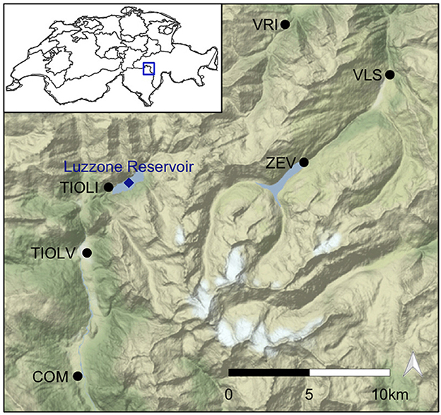
Figure 1. Study site with locations of precipitation stations and Luzzone reservoir.

2.1. Study site

The study site includes the Luzzone reservoir (46°34′00″N; 08°58′45 ″E), which is part of the Blenio hydropower network in the canton of Ticino in Switzerland. The reservoir is roughly 1.27 km² in surface area and is located at an altitude of ~1,590 m.a.s.l within a catchment area of about 36.7 km². The reservoir is naturally fed by various mountain streams, primarily the Ri di Luzzone from the east, Ri di Scaradra from the south, and Ri di Cavallasca form the north. Water from the neighboring Carassina reservoir (46°32′47″N; 08°58′01″E, located at an elevation of 1,705 m.a.s.l.) is also directed into the Luzzone reservoir. This Luzzone outflow is managed and used by various energy providers to generate electricity.

The meteorological station nearest to the Luzzone reservoir is called Olivone diga Luzzone (short name TIOLI), and is located at the north-western corner of the reservoir (46°33′54″N; 08°57′38″E) at about 1,617 m.a.s.l. Additional stations located in Ticino and in Graubünden are also included (Figure 1). The coordinates of each station are provided in Supplementary Table 1.

2.2. Data

2.2.1. Precipitation

Precipitation data was acquired from the MeteoSwiss automatic monitoring network through the IDAWEB (2019) portal. Daily precipitation totals from January 1st, 2000 to present day are available for the TIOLI site. The gauge at the TIOLI station was fitted with a heater in 2008, so to maintain consistency in the measured data used, only data collected after 2008 are used in this study. The raw dataset had 15 missing values. The set included daily totals measured from 6 UTC to 6 UTC following day. The data from 2009 through 2020 are displayed in Supplementary Figure 1. For a more comprehensive analysis, stations with longer useable precipitation data are included. The full data sets are freely available through the IDAWEB (2019) online platform of the Federal Office of Meteorology and Climatology MeteoSwiss.

2.2.2. Inflow

Daily total inflow data for Luzzone were provided by BKW Energie AG for the full years of 2000 to 2019. The daily values of inflow were back-calculated from measured reservoir volumes and changes in input/output. Due to the nature of this data the inflow is a bulk sum of inputs to the reservoir and cannot be considered exclusively as streamflow. As the inflow values were not directly measured, there is some uncertainty in the accuracy of the exact values. For instance, the level of sediment build-up in the reservoir over this time (which would have altered the total volume) was not known and thus could not be accounted for. Most of the data are consistently under the below 4,000 (10³ m³) with the exception of one single-day outlier value in 2008 (Supplementary Figure 1). Additionally, the raw data for inflow included negative inflow values, which have no physical meaning. Thus, linear interpolation was applied to the negative values in the timeseries to bring them into the positive space and allow for more meaningful interpretation. The monthly distribution of inflow follows a bell shape, with most occurring in late spring through the fall season, but peaking in summer.

2.3. Methods for heavy precipitation and high inflow

In order to calculate expected recurrences of extreme high precipitation and inflows, the traditional extreme value approaches are applied. Given the short length of the precipitation and inflow datasets (10–20 years), alternative approaches adapted for application to small datasets were also applied. Here a brief overview of two traditional extreme value analysis methods and two newer methods is provided. Details about extreme value approaches are nicely summarized in the review by Nerantzaki and Papalexiou (2022).

2.3.1. Extreme value analysis: generalized extreme value distribution and generalized pareto distribution

The traditional methods for extreme value analyses require the separation of the “extreme” values from the rest of the data. The sub-setting of the data can be done either by selecting block maxima or minima (BM) from each defined period or based on points over (or under for minima) a threshold (peak-over-threshold, POT). As explained by Coles et al. (2001), the family of generalized extreme value (GEV) distributions is used for BM data (Fisher and Tippett, 1928), while the generalized pareto distribution (GPD) is often applied to POT data (Balkema and de Haan, 1974; Pickands, 1975). The corresponding cumulative distribution function (CDF) of the GEV and GPD, respectively, are:

$\begin{array}{ll}P\left(X\le x;\mu ,\sigma ,\xi \right)=\{\begin{array}{c}{e}^{-\left({1+\xi \left(\frac{x-\mu }{\sigma }\right)}^{-\frac{1}{\xi }}\right)},if\xi \ne 0\\ e^{-\left(e^{-\left(\frac{x-\mu }{\sigma }\right)}\right)},if\xi =0\end{array}& (1)\end{array}$

$\begin{array}{ll}P\left(Y\le y|Y>u;{\sigma }_u,\xi \right)=\{\begin{array}{c}1-\left(1+\xi \left(\frac{y-u}{{\sigma }_u}\right)\right),if\xi \ne 0\\ 1-e^{-\frac{y}{{\sigma }_u}},if\xi =0\end{array}& (2)\end{array}$

where X are the annual maxima and Y are the daily values. The GEV distribution (Equation 1) can be characterized by μ, σ, and ξ, denoting location, scale, and shape parameters, respectively. The GPD (Equation 2) has two parameters, σ_u and ξ. It has an additional term, u, representing the threshold beyond which the peaks are considered.

Return levels can be determined directly from the inverse of the CDF (inverse function, not to be confused with multiplicative inverse). This is shown in the following:

$\begin{array}{ll}{z}_{GEV}\left(N\right)=\{\begin{array}{c}\mu -\frac{\sigma }{\xi }\left[{1-\left\{-log\left(1-\frac{1}{N}\right)\right\}}^{-\xi }\right],if\xi \ne 0\\ \mu -\sigma log\left\{-log\left(1-\frac{1}{N}\right)\right\},if\xi =0\end{array}& (3)\end{array}$

$\begin{array}{ll}{z}_{GPD}\left(N\right)=\{\begin{array}{c}u+\frac{\sigma }{\xi }\left[{\left(Nn{\zeta }_y\right)}^{\xi }-1\right],if\xi \ne 0\\ u+\sigma log\left(Nn{\zeta }_y\right),if\xi =0\end{array}& (4)\end{array}$

where N represents the return period (e.g., N = 100 for a 100-year return period) and n represents the number of data points collected within the time periods (e.g., n = 365 for daily data). ζ_y represents the probability that an event exceeded the threshold, u, which can be written as ζ_y = Pr(X > u) and estimated as $\frac{k}{n}$, where k is the number of excesses and n is the total sample size.

Note that the z_GEV term represents the return level (Equation 3), which has the expectation of being exceeded once per the return period or every N-years. Similarly, for the GPD, Equation (4) shows the return level, z_GPD, which can be expected to be exceeded on average once every N-years.

An added consideration for the GPD case is that some data points might be part of the same event and falsely attribute greater frequency to that event. In order to only select independent events, the data above the given threshold are declustered before the GPD fitting is applied (using the extRemes package in R, Gilleland and Katz, 2016). Within this function, the method for declustering used was an intervals estimator (Ferro and Segers, 2003). The results from the declustered GPD (GPDd) case are included alongside the non-declustered GPD method.

2.3.2. Extended generalized pareto distribution

Both the GEV and GPD approaches are widely used, but have the disadvantage of further limiting the available dataset for analysis by only considering extreme values. Therefore, newer approaches, which make use of all available datapoints of an event (zeros excluded), have been proposed and successfully applied (e.g., Papastathopoulos and Tawn, 2013; Naveau et al., 2016; Evin et al., 2018; Tencaliec et al., 2020; Rivoire et al., 2021; Haruna et al., 2022). Here we apply the extended generalized pareto distribution (eGPD), through an open-source code in R (R Core Team, 2021). It was developed by Naveau et al. (2016) initially for application to both high and low non-zero rainfall extremes, but it can be applied to any heavy-tailed distribution.

The idea was to overcome the need for threshold selection in the generalized pareto by defining a unifying gamma-like density function, which is in compliance with extreme value theory for both the upper and lower tail of the distribution.

$\begin{array}{ll}P\left(Y\le y\right)=\{\begin{array}{c}1-cst\times {\bar{H}}_{\xi }\left(\frac{y}{\sigma }\right),foranylargey\\ cst\times y^k,foranysmally\end{array}& (5)\end{array}$

This led Naveau et al. (2016) to propose the CDF of the daily values:

$\begin{array}{ll}P\left(Y\le y\right)=F\left(x\right)=G\left\{H_{\xi }\left(\frac{y}{\sigma }\right)\right\}& (6)\end{array}$

where G is a continuous CDF on [0,1] that has to follow different constraints detailed in Naveau et al. (2016) so that the upper tail is preserved and the lower values behave like y^k.

The N-year return level, can be computed from Equation (6) for a given G based on the inverse of the CDF (G⁻¹):

$\begin{array}{l}\hfill z_{eGPD\left(N\right)}=F^{-1}\left(1-\frac{1}{N{n}_p}\right)=\hfill \\ \{\begin{array}{c}\frac{\sigma }{\xi }\left[{\left\{1-G^{-1}\left(1-\frac{1}{N{n}_p}\right)\right\}}^{-\xi }-1\right],if\xi >0\\ -\frac{\sigma }{\xi }log\left\{1-G^{-1}\left(1-\frac{1}{N{n}_p}\right)\right\},if\xi =0\end{array}& (7)\end{array}$

where σ is the scale parameter, ξ is the shape parameter while n_p represents the mean number of positive data points per year. The shape parameter determines whether the GPD is exponential or light-tailed (ξ = 0), or heavy-tailed (ξ > 0). Heavy rainfall is often exponential or heavy-tailed (Katz, 2002; Naveau et al., 2016). Naveau et al. (2016) proposed four parametric families that may represent G. The model used in this study was:

$\begin{array}{l}G\left(v\right)=v^k,threeparameterfamilywhere\kappa >0;\end{array}$

Here κ and ξ are the shape parameters for the behavior of the lower tail and upper tail of the distribution, respectively.

2.3.3. Metastatistical extreme values distribution

Finally, another approach for assessing extreme values is the Metastatistical Extreme Value (MEV) distribution, which was introduced by Marani and Ignaccolo (2015) with the aim of easing the requirement of the asymptotic assumption in traditional extreme value analysis.

Similar to the eGPD, the MEV uses all of the available values in a dataset and specifically focuses on including data points making up both ordinary and extreme events. The number of ordinary events, n, are considered by block (e.g., n is the number of rainfall days per year). As explained by Zorzetto et al. (2016), the extremes of the dataset emerge from repeated sampling of all ordinary points, so the statistical parameters themselves have a distribution that describes the behavior of the data. Thus, the number of events per block, n, and the parameter values for the distribution of each block, are realizations of stochastic variables (N and $\vec{\Theta }$, respectively). From Marani and Ignaccolo (2015), the cumulative MEV for annual maxima is expressed as follows:

$\begin{array}{ll}P\left(X\le x\right)=H\left(x\right)={{\displaystyle \sum }}_{n=1}^{\infty }{\displaystyle {\int }_{{\Omega }_{\overrightarrow{\Theta }}}}{\left[F\left(x:\vec{\theta }\right)\right]}^{n}g\left(n,\vec{\theta }\right)d\vec{\theta }& (8)\end{array}$

where ${\Omega }_{\vec{\Theta }}$ is the set of possible parameter values of F (parent distribution), $\vec{\theta }$ represents the parameters of F, and g(n, $\vec{\theta }$) is the joint probability distribution of the number of events and parameters, which are realizations from N (discrete values) and $\vec{\Theta }$ (continuous), respectively.

The MEV has since been applied to numerous studies investigating precipitation extremes (Zorzetto et al., 2016; Marra et al., 2019; Schellander et al., 2019; Miniussi and Marani, 2020; Miniussi et al., 2020; Zorzetto and Marani, 2020). The authors of the listed studies that used the MEV method for precipitation timeseries found their data followed a Weibull distribution [which is consistent with findings by Wilson and Toumi (2005) for heavy precipitation events] and thus their use of the MEV has been adapted accordingly. Zorzetto et al. (2016) shows this by first averaging over the empirical frequency distribution of the parameters, $\vec{\Theta }$:

$\begin{array}{ll}H\left(x\right)=\frac{1}{T}{{\displaystyle \sum }}_{j=1}^T{\left[F\left(x:{\vec{\Theta }}_j\right)\right]}^{n_j}& (9)\end{array}$

where T is the number of years and n_j is the number of daily precipitation events in year j. Thus, each year of data becomes one realization of $\vec{\Theta }$, N.

Where the daily data can be assumed to follow a Weibull distribution then from Marani and Ignaccolo (2015) and Zorzetto et al. (2016) the MEV can be approximated as:

$\begin{array}{ll}H\left(x\right)=\frac{1}{T}{{\displaystyle \sum }}_{j=1}^T{\left[{1-exp}^{{-\left(\frac{x}{C_j}\right)}^{w_j}}\right]}^{n_j}& (10)\end{array}$

For the Weibull distribution, the scale and shape parameters are represented by C_j and w_j, respectively, as the parameters are estimated for each year, j ε{1,…,T}, of data. Similarly, n_j is the number of ordinary events in each year. Note, for the data of daily precipitation and inflow, the Weibull distribution is initially assumed.

As described by Schellander et al. (2019) if the data can be assumed to be time-invariant, then the parameters can be estimated from the collective dataset directly (i.e., C_j = C, w_j = w) and n_j can be averaged across the years to become $\bar{n}$ (the average number of ordinary events per year). This gives a simpler version of the MEV:

$\begin{array}{ll}H\left(x\right)={\left[{1-exp}^{{-\left(\frac{x}{C}\right)}^w}\right]}^{\overline{n}}& (11)\end{array}$

Schellander et al. (2019) note that this formulation of the MEV has been proposed by Marra et al. (2019) and is called the simplified MEV (SMEV).

As with the GEV and GPD approaches, quantiles (or inverting the CDF) can be used to generate the return levels for given return periods as:

$\begin{array}{ll}{z}_{MEV\left(N\right)}=H^{-1}\left(1-\frac{1}{N}\right)& (12)\end{array}$

2.4. Method for low precipitation and inflow events

For determining the return periods of low inflow and dry periods, an alternative approach was used. The low rainfall and low inflow cases were examined empirically, without any parametric model fitting. We use the term “low inflow” for the total reservoir inflow to distinguish it from “low flow” which commonly denotes low river discharge (Van Loon, 2015).

Since low inflows/low precipitation events are particularly impactful based on event duration rather than just single day magnitudes, the first step was to identify the low events and their duration. To this end, the data were transformed into discrete counts of consecutive low input days. For the precipitation case, these were days with total precipitation of 0 mm day⁻¹. For the inflow case, a low inflow threshold value (u) based on the 7.5th percentile was selected, where days with flows below u were considered to be low inflow days. Both of these are constant-type thresholds. The fixed threshold was used for inflow because it was specific to a storage hydropower reservoir, with the implication that below a certain threshold the turbines of the power station cannot operate. Notably, this hard limit is not known to the authors and thus a low percentile value of the dataset was used.

The reservoir receives natural inflow from streams but also engineering inflow directly from another managed storage reservoir. The high level of water management, means that there is generally less variability than in rivers as operators manage the water based on anticipated demand and projected inflows over the seasons. To try to gain a better understanding of the natural seasonal changes, we included different thresholds per season as well as the annual one. As inflow is not directly measured, but rather back calculated from the daily water level in the reservoir, we could not confidently estimate the contribution of separate inflow sources, but could only use the calculated estimate of inflow. Provided the streamflow contributions to the reservoir are known, a variable threshold method (Heudorfer and Stahl, 2017) could be applied as this may give a more characteristic representation of dry periods in the contributing variable inflow sources. The corresponding return levels for the various thresholds are summarized in Supplementary Table 2. Following the threshold selection, consecutive days of low inflow were aggregated, counted and the new discrete dataset was used to characterize the low inflows by event lengths or “dry spells”.

The length of a low inflow event is sensitive to u in the sense that if u were increased, then more days would appear below this u value and the longest consecutive low inflow event will increase in duration compared to a case with a lower u.

To determine the return levels for a dry spell, the assumption was made that the sequences of consecutive low events are independent. Then the return period of a sequence of consecutive low inflow days of length, L, greater than or equal to a value of interest, a, could be expressed as:

$\begin{array}{ll}T\left(L\ge a\right)=\frac{1}{m\times P\left(L\ge a\right)}& (13)\end{array}$

Where m (the average number of dry spells of any length per year) is multiplied by the probability of an event lasting as long as or longer than a number of days. The probability is found based on the Weibull plotting position formula (Makkonen, 2006). It is calculated by first ranking the historical dry spells (of each length) by frequency and then dividing each rank by the sum of one plus the total number of all dry spells.

In order to determine the return level at a given return period, the probability of an event lasting more than a days was determined by the rearrangement of Equation (13):

$\begin{array}{ll}P\left(L\ge a\right)=\frac{1}{m\times T\left(L\ge a\right)}& (14)\end{array}$

Results for low inflow for different return periods were estimated using 10 years of data and again using 20 years of data and can be seen in Figures 5, 6, respectively. The same was done for low precipitation at the TIOLI and TIOLV precipitation stations and return level values are summarized for 10- and 20-year return periods in Supplementary Table 2.

A limitation of this approach is that the results are bounded by the lowest and highest return periods. Intermediate return periods for which there was no exact record in the data could be estimated by linear interpolation between existing data points. In order to get a more comprehensive event-length estimate, the data set was bootstrapped (see below) and the mean count level of all runs was used as the expected count level to be matched or exceeded in the return period of interest.

2.5. Confidence intervals

Confidence intervals for the return levels obtained with each method were determined by bootstrapping the data 1,000 times with replacement. A block bootstrapping approach was applied to the GPD, declustered GPD, eGPD, MEV and low inflow/low precipitation results. This was done by shuffling the months of data instead of shuffling the days in the dataset. This way, the uncertainty estimate would react more strongly if there was significant temporal dependence in the data. Since the GEV uses only the maxima of each period, a simple bootstrap of maxima shuffled across all days was acceptable.

2.6. Software packages used

Fitting for all high inflow and precipitation extremes was done in the R program (R Core Team, 2021). Maximum likelihood estimation (mle) was used to fit the GEV, GPD, eGPD, and MEV. For the GEV, the extreme value distribution, evd (Stephenson, 2002), package was used with the “fgev” function by maximum-likelihood fitting of the GEV. For the GPD the “fpot” function from the same evd package was used. For the declustered GPD case, the modification to “decluster” the data was applied using the extRemes package (Gilleland and Katz, 2016) to make excesses more independent. For the eGPD model, the “extgp” function from the mev package was used (Belzile et al., 2020). For the MEV, the mevd package was used (Schellander, 2020). For the precipitation cases, the “simple” type (SMEV, Equation 11) was used, while for the inflow case the “annual” type (Equation 10) was found to yield a better fit. For consistency with the other methods, the eGPD and the MEV parameters were estimated using maximum likelihood estimation (mle), although the authors acknowledge that the probability weighted moments (pwm) approach is recommended for these methods by both Naveau et al. (2016) and Schellander et al. (2019), respectively.

3. Results

The results are presented below according to the cases investigated - first with respect to heavy precipitation and high inflow and then for dry spells of low precipitation and low inflow.

3.1. Heavy precipitation

Return level plots for heavy precipitation at the TIOLI station near the Luzzone reservoir (as determined using the GEV, GPD, GPD with declustering, eGPD, and MEV) are shown in Figure 2. All of the methods (GEV, GPD, eGPD, MEV) give similar representation of the upper tail, though the GEV has the steepest increase at high return periods. The smallest difference is between the declustered and non-declustered GPD.

FIGURE 2

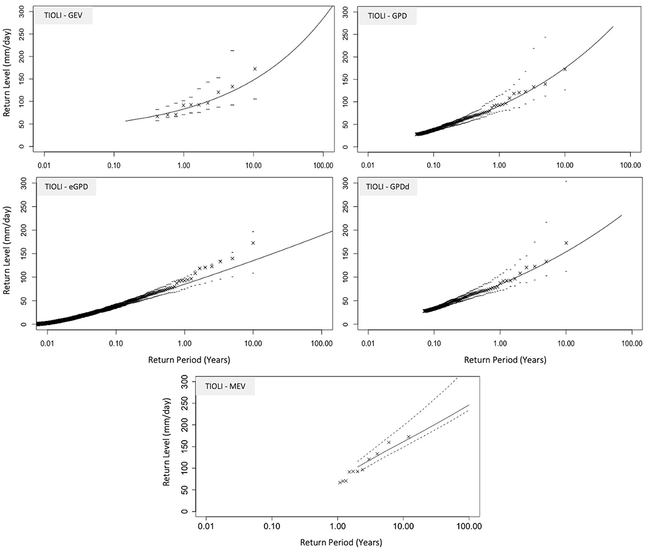
Figure 2. Return level plots for TIOLI precipitation using, GEV, GPD, GPDd (declustered), eGPD, and MEV (Weibull distribution applied), based on 10-years of daily precipitation data; upper (97.5 percentile) and lower (2.5 percentile) confidence bands obtained from bootstrapping 1,000 runs.

Twenty-year return levels for all of the stations in the study region calculated for the annual case using 10-, 20-, and 40- years are shown in Figure 7. Though the TIOLI and COM stations only had a maximum of 10 and 20 years (respectively) available, it is evident that all methods tend toward similar return level results as more data becomes available. The largest variations between the method-specific return levels appear in the 10-year datasets, with the GEV resulting in visibly lower return levels than all other methods.

3.2. High inflow

Figure 3 shows the results of various statistical approaches for determining the return levels of high inflow events. Visually, the GEV, GPD, GPD with data declustering, and eGPD provide results that represent the observations fairly closely, particularly for the higher returns. As with the precipitation case, the declustering of the data does not appear to significantly improve the fit compared to the non-declustered GPD. In contrast, results from the MEV, deviated much more from the observed returns.

FIGURE 3

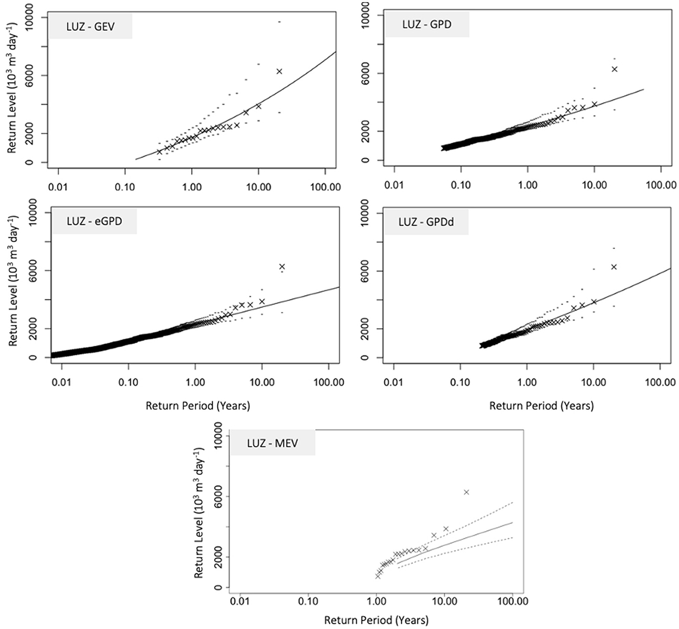
Figure 3. Return level plots for LUZ reservoir inflow using, GEV, GPD, GPDd (declustered), eGPD, and MEV (Weibull distribution applied), based on 20-years of daily inflow data; upper (97.5 percentile) and lower (2.5 percentile) confidence bands obtained from bootstrapping 1,000 runs.

Twenty-year return levels for the reservoir inflow calculated for the annual and seasonal cases, based on timeseries of 10 and 20 years are shown in Figure 8. The longer timeseries does shows a small improvement in the agreement of return level values between the methods. Unlike the precipitation data, the MEV rather than the GEV provides the lowest return level. This is particularly clear in the summer and fall seasons, as well as in the annual data series.

3.3. Low precipitation

The results for low precipitation are presented in Figure 4. The return levels are given for annual and seasonal cases and represent the original data only (not the bootstrapped runs). For precipitation at the TIOLI station, the longest recorded events lasted, 24, 21, 17, 14, and 21 days long for the annual, winter, spring, summer and fall series, respectively. Across all return periods, the maximum event lengths are seen in the annual series. This was expected because low precipitation sequences can extend between the different seasons. For the seasonal series', the longest dry events are seen in the winter season while the shortest low precipitation events all occur in the summer season.

FIGURE 4

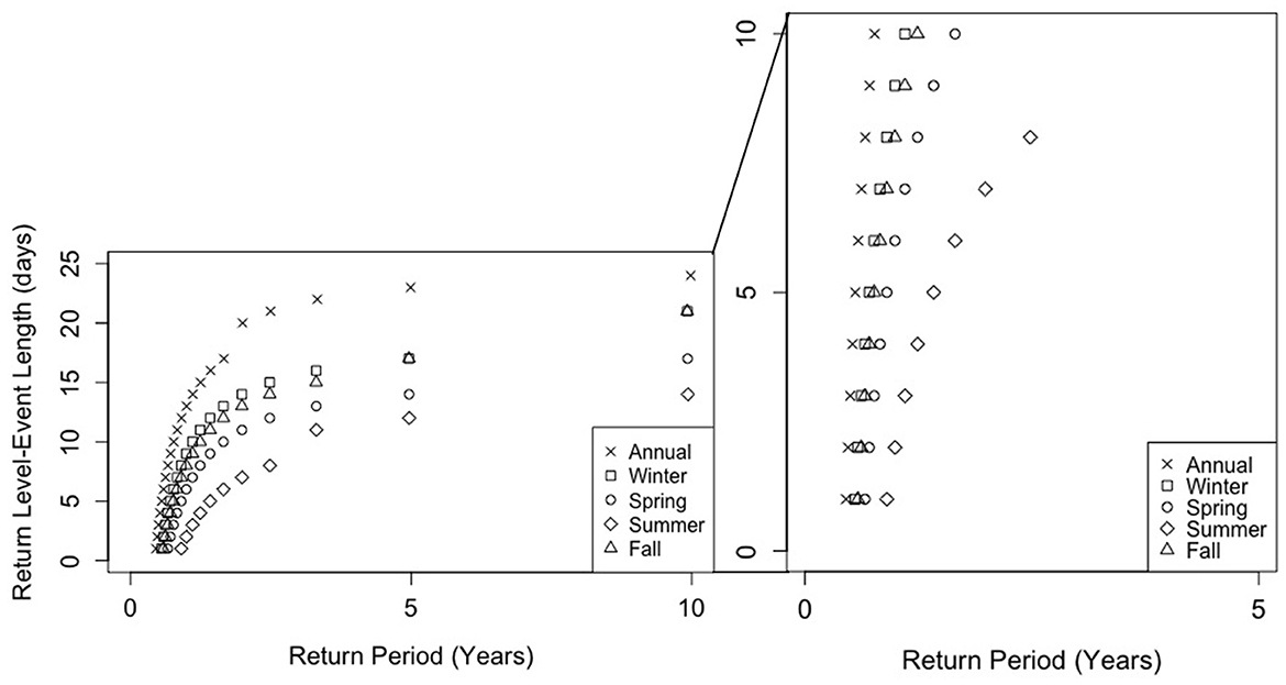
Figure 4. Low precipitation return levels (event length) for annual and seasonal cases based on 10 years of data at TIOLI station.

3.4. Low inflow

Low inflow events were defined using the 7.5th percentile of each series (annual vs. season-specific) as a cut-off threshold. Figure 5 results were computed using only the latest 10 years of inflow data while Figure 6 results are based on 20 years of data. In both Figures 5, 6, the top left plots use threshold percentiles that are specific to each season, whereas the bottom and the rightmost plots use the same threshold (summer percentile) for all seasons. All threshold values can be viewed in Supplementary Table 2.

FIGURE 5

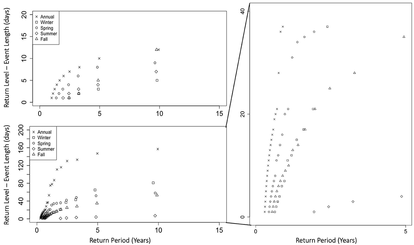
Figure 5. Low inflow return levels (event length) for annual and seasonal cases based on 10 years of data; lower 7.5th percentile of each case used for thresholds (top left); using 7.5th percentile of summer season as threshold for all cases (bottom and right).

FIGURE 6

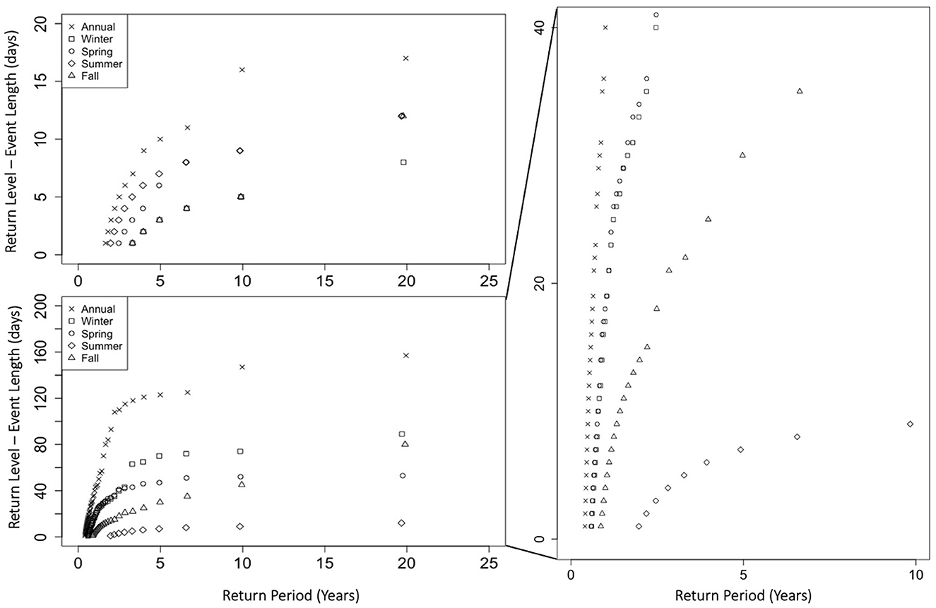
Figure 6. Low inflow return levels (event length) for annual and seasonal cases based on 20 years of data; lower 7.5th percentile of each case used for thresholds (top left); using 7.5th percentile of summer season as threshold for all cases (bottom and right).

As with the low precipitation events, the longest low inflow events consistently occurred in the annual series for each return period, which is expected because there are no truncations of the events in the annual series. Similarly, in the seasonal cases, when the threshold was consistent, the longest low inflow events occurred in winter while the shortest occurred in summer.

3.5. 20-year event profiles

From the results presented above, a profile of event return levels with a 20-year return period (chosen to correspond to the length of the inflow data-set) was generated. The results for high precipitation (Figure 7) and high inflow (Figure 8) events are shown with unique markers indicating the bootstrapped mean 20-year return level obtained through the different methods. Figure 7 depicts only the annual cases (not seasonal) for six different stations using various lengths of the datasets. Figure 8 also includes the seasonal cases as well as return levels for low inflow, calculated with the non-parametric method. Since this method does not allow for the maximum return level to exceed the data length, the 10-year return levels are presented rather than 20-year levels. In all panels of the profiles, upper and lower confidence intervals are the 97.5th and 2.5th quantiles of the bootstrapped mean return levels. Depicting the results as a profile with separate panels for each case provides a snapshot of the return levels for a recurrence period of interest for each process (precipitation or inflow). This presentation allows for clearer view of specific return periods of interest for each case.

FIGURE 7

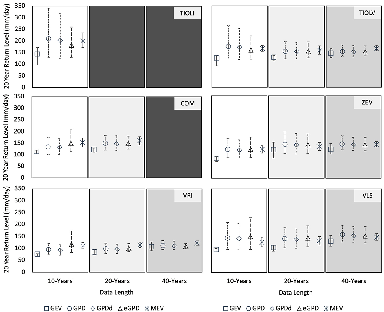
Figure 7. Twenty-year return levels of daily heavy precipitation for study site stations using parameter estimates from 10-, 20-, and 40- years of data for each method (GEV, GPD, GPDd, eGPD, and MEV); confidence intervals based on 97.5th and 2.5th percentiles from 1,000 bootstrapped samples.

FIGURE 8

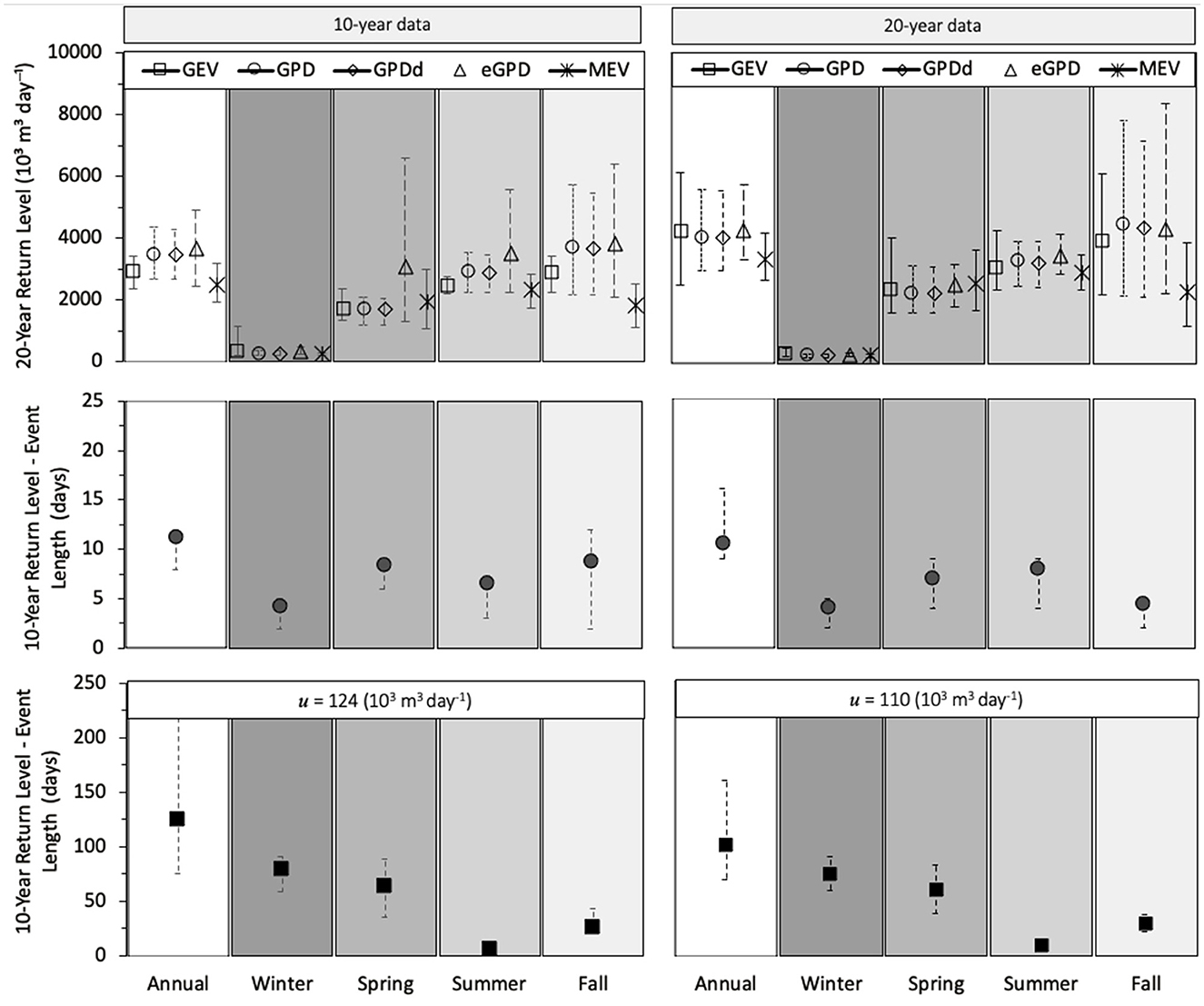
Figure 8. (Upper) 20-year return levels of daily high inflow for Luzzone reservoir using parameter estimates from 10- and 20-years of data for each method (GEV, GPD, GPDd, eGPD, and MEV); (Middle): 10-year return levels of events defined by 7.5th percentile threshold specific to each season; (Lower) 10-year return levels of events defined by 7.5th percentile of summer season; confidence intervals based on 97.5th and 2.5th percentiles from 1,000 bootstrapped samples.

3.5.1. High precipitation and inflow extremes

The top panels of Figure 8 show that the 20-year return levels calculated using the various methods of GEV, GPD, declustered GPD, eGPD, and MEV are generally comparable when considered within the same time series (e.g., annual vs. season-specific), with some clear exceptions. The MEV return level differs the most from the other methods, but particularly in the fall season for the inflow case, regardless of data length. Following the MEV, the GEV result differs from the GPD-based results, also most noticeably in the fall case. Generally, larger discrepancies are seen between return levels determined by different methods when short datasets are used. This is evident for both the processes of precipitation and reservoir inflow. For the precipitation cases, the GEV is most clearly affected by the data set length. For inflow, the seasonal cases depicted show that all methods give the largest variability during the fall season. As with precipitation the annual values are similar between the GDP and eGPD methods, while the GEV and MEV diverge, particularly with the shorter dataset. In addition, the eGPD value is most different from the rest of the methods in the spring and summer when the 10-year data set is used.

3.5.2. Low precipitation and inflow events

In the remaining panels of Figure 8, the 10-year return levels for low inflow are reported for cases where thresholds are based on the lower 7.5th percentiles of each season (middle panels) and for cases where the summer season threshold (u) was used for all cases. Regardless of whether 10 or 20 years of data where used, the return levels based on the consistent thresholds gave similar results. Expectedly, where the threshold was unique to each season, the results in summer and fall varied with the length of the dataset used. Low precipitation events for the TIOLI and TIOLV stations were also calculated across seasons and for different dataset lengths (10–40 years) for 10- and 20-year return levels. These results also used a fixed threshold (0 mm day⁻¹) and yielded a similar relationship in seasonal return levels as the fixed inflow cases for all dataset lengths. These low inflow and low precipitation results are summarized in Supplementary Table 2.

4. Discussion

4.1. High precipitation and inflow

The initial motivation for this study came from the aim to use the most appropriate method to calculate return levels of impactful precipitation and inflow events of small (10 or 20-year) datasets, using the particular case of data relevant to changes in hydropower reservoir fill-levels. The key differences between the methods comes from the treatment of the dataset, rather than just the method applied. For instance, the GEV and GPD only focus on the extreme values of the data. The eGPD and MEV use extreme values but also include ordinary values and thereby the additional information that comes along with them. Therefore, for high precipitation and high inflow, it was expected that the eGPD and MEV methods would yield different results than the traditional approaches of the GEV and GPD methods. This would be in line with previous studies, such as Zorzetto et al. (2016), who found the MEV to outperform the GEV, particularly for cases where the return period of interest was longer than the length of the dataset.

Indeed, examining the annual cases of precipitation the GEV return level is consistently lower than all other methods for every station, but approaches the other return level values as the dataset length increases. In these cases, the MEV was similar or very slightly larger than the other method results. However, it did not appear to be distinctly different. In contrast, the MEV for inflow was clearly lower than the other methods for the annual case and particularly for the fall season regardless of the data length. This particular discrepancy (as discussed further below) can be attributed to the Weibull distribution being an ill-fit for the inflow data, while it fit very well for the precipitation data. The GEV however, is most sensitive to the dataset length compared to the other methods for both inflow and precipitation.

The results of the inflow cases showed that, while there were similarities in the values from each method for the winter series (where flows historically have been less variable), there were discrepancies in the other seasons and in the annual series. Notably, the annual precipitation results showed that the eGPD, GPD/GDPd, and MEV results were more similar in value, even in shorter datasets. Given the similarity in return level results, this would indicate that the peak-over-threshold parsing of extremes (to which the GPD is applied) provides as sufficient an amount of information as the more data-inclusive approach (for the eGPD) for these cases. One more point of comparison is the similarity in the results of the GPD applied to the declustered and non-declustered data. In the high precipitation and high inflow cases, the resulting return levels were not very different, however, it may still be relevant for other datasets and should be assessed on a case-by-case basis. Overall, the similar return levels indicate that the inclusion of ordinary events does indeed make a difference against the alternative of the block maxim/GEV method but not necessarily against the POT/GPD approach.

The largest difference when method results are compared in the inflow cases was from the MEV. This method uses all ordinary positive values, as the eGPD, but a Weibull distribution is applied in this formulation. This distribution is often valid for precipitation data and has been successfully applied in other studies of extreme precipitation. Similarly, it did provide as good of a fit as the GPD in this precipitation case (Figure 2). This also resulted in an acceptable annual return level in Figure 7. For inflow, the poorer fit from the MEV is seen in Figure 3 as the model underestimates the data behavior. The resulting, lower return levels are evident in Figure 8. The poor fit for the inflow also occurs in the corresponding seasonal series. This was not as surprising for the inflow case because other distributions could better represent the data and this is clearly an important element in the MEV process. This indicates, that when the season-specific cases are examined, the model may be more sensitive to the smaller amount of data and that these data should be also be represented by a different distribution that better reflects the data patterns in each season.

It is important to note that the resulting shape parameters for the same data, calculated by different methods, were different (please see Supplementary Tables 3, 4). Shape parameters indicate if a distribution has a heavier or lighter tail. Heavier tails indicating greater frequency and intensity of extreme events (e.g., Papalexiou and Koutsoyiannis, 2013; Papalexiou et al., 2013). Most methods yielded positive shape parameter values for all seasonal and annual cases. Only the GEV method gave negative values for most cases of precipitation and for the 10-year summer inflow case and tended to underestimate the return levels compared to the other methods. This is similar to results found by Moccia et al. (2021a,b), who found the Weibull distribution to underestimate the returns.

In general, for high precipitation and high inflow cases, it can be recommended that—for a small dataset—the eGPD can be selected although the classic GPD (declustering by case) also can yield acceptable results if not too many data points are lost by the threshold selection process. The GEV, however, is not recommended for use in estimating return levels for small datasets. The MEV is recommended to be selected over the GEV, and possibly over the GPD, but only with the correct distribution for the specific data.

4.2. Low precipitation and inflow

As with the high precipitation and high inflow cases, the results from the low precipitation (Figure 4) and low inflow (Figures 5, 6) cases also show that the temporal series under consideration makes a difference in the resulting return level, as expected. For both cases, the annual return levels were consistently higher than the seasonal levels. This is because of the way that the events were selected. It is standard practice to view seasonal differences by splitting the annual data set into corresponding calendar months. The benefit is a consistent split, but it comes at the cost of possibly breaking up an event. Due to this effect, it is recommended that the annual series be viewed in addition to the seasonal series when the calendar months are used to subset the data. The annual series will provide the full length of historical maxima, while the seasonal split will give an indication in which season the majority of an event can be expected.

For the low precipitation, the summer season provided the shortest low precipitation event length. This may be attributed to the seasonally warmer temperatures allowing for more moisture in the air, which enables more precipitation in general. The winter and fall season have the longest low precipitation spells, which is to be expected with the colder temperatures prohibiting the same amount of moisture to be held as in the warmer seasons (although this may differ in the future with climate change).

The low inflow case, where thresholds were uniformly based on the 7.5^th summer percentile tended to follow a similar seasonal relationship as precipitation, with the longest events appearing in winter and the shortest occurring in summer. This was less clear when inflow events were based on threshold values that are unique to the seasonal and annual series. This second approach can offer a helpful view for reservoir management when interested in return-levels based on historical expectations of inflow during a specific time/season, but the former approach is generally easier to interpret. As with the low precipitation case, the longest low inflow event occurs in the annual series. This is to be expected because the moderate annual threshold value allows many more days from which to draw than just the seasonal series. With generally higher precipitation occurring in summer as compared to the winter (e.g., Rysman et al., 2016), it was expected that inflow levels in the same location would be higher and so the low inflow events would be shorter. The understanding of the inflow patterns could be furthered with additional information about the individual sources contributing to the reservoir inflow volume. Contributions to the natural inflow do include precipitation, stream flows, and snowmelt, but without additional types of data (e.g., measured stream flow), the actual contributions of these sources of these inflow values remain speculative.

4.3. Limitations

Each method applied in this study has its strengths and weaknesses. The block maxima/minima definition of extremes, for which the GEV is commonly used, is well-established and straightforward to apply. However, the basic assumptions (e.g., asymptotic assumption) can make the method questionable for application to smaller datasets as the block maxima selection further reduces the available data size. The GPD, where peak data over a threshold are used, allows for less data to be discarded. Declustering the data beforehand is done to ensure statistical independence between events, a requisite of EVT. The key limitation is in the selection of an appropriate threshold (to find an optimum between variance and bias), although methods to aid in the selection procedure do exist (Scarrott and Macdonald, 2012). Even so, the threshold-based approach also reduces the existing dataset.

The eGPD and the MEV are within the family of methods that aim to make use of all positive data and thereby address the main limitations of the previous approaches of dataset size limitations. Yet they also have a few limitations. A drawback of the eGPD is that without appropriate censoring of the likelihood the fits are poor. Further, the fit of the eGPD is quite sensitive to the selected value for the censored likelihood process. Similar to the threshold selection for the GPD, an appropriate value can be selected based on visual inspection of the model fit against the empirical data in a quantile-quantile plot. Alternatively, the value giving the smallest root mean squared error (RMSE) between the fit and the empirical data can be used. The main limitation of the MEV is that the correct distribution of the data should be first determined and then applied within the MEV framework. This can certainly be done, but is not as straightforward as the other approaches for practitioners desiring a rapid calculation of return levels. However, as the method becomes more know over time, it may likely be applied more often because of the flexibility of the approach.

A general limitation that is relevant for all of the approaches is that they are purely based on one set of historical data and thereby restrict the calculation of return levels or return periods to those expected based on previous events. Thus, the results should be interpreted with care, particularly in a changing climate because the climate change influence is not explicitly identified. As a consequence, these methods cannot be used for forecasting, although they might be useful in informing expectations within a short timeframe in the future (e.g., couple years ahead).

Stemming from this, the perspective of the return levels taken from the annual view of the data differs significantly from the view taken based on seasons. Insight into how the return levels differ in winter as opposed to summer, for instance, can be useful for practitioners curious about the variations of return level expectations throughout the year. It is common for only the annual view to be taken, but this does not indicate when in the year the return level is anticipated to occur. In fact, as shown, the differences in the seasonal vs. annual return levels in the cases examined were quite large for both the high and low inflow cases. This indicates the importance of the timeseries selection along with the appropriate method choice.

5. Conclusions

Based on the results of this study, we can conclude with the following messages. Heavy precipitation, high inflow, and dry spells are all events that can impact reservoirs and thereby related hydropower production. Estimating the expected return of each event requires that the most appropriate view of the data is taken and that the most relevant method is applied. It can be concluded, that for the cases of high precipitation and high inflow, the method selected can make a difference in return levels and that particular care should be taken when applying the methods to the seasonal vs. annual timeseries. The GEV and GPD have long been in use, but they come with the drawback of reducing the data in the analysis, which is problematic when the data is limited. This is a particular weakness for the GEV, which is not recommended for use with small datasets. In such cases, the eGPD or MEV may be more beneficial than traditional models. However, it is critical to ensure that the correct distribution is applied in the case of the MEV and that an appropriate censored likelihood selection is made in the case of the eGPD. These selections must be tailored to the timeseries (seasonal or annual). When correctly applied they can be used for smaller datasets (e.g., 10-years) as well as longer ones. For low precipitation and low inflow events, the series under consideration makes a large impact on what return levels can be expected for a given return period. In addition, the application of a specific threshold value is important to consider as it can change the meaning of the resulting low event return levels. Overall, it is recommended that the treatment of the data be considered on a case-by-case, with particular attention to the dataset length and type (inflow vs. precipitation) to ensure that the most appropriate method is applied.

Data availability statement

The data presented in the study are deposited in the EnviDat repository, and can be found here: https://www.doi.org/10.16904/envidat.415.

Author contributions

TM: conceptualization, methodology, writing—original draft preparation, and writing—reviewing and editing. JB: methodology and writing—reviewing and editing. ML: conceptualization, writing—reviewing and editing, and supervision. All authors contributed to the article and approved the submitted version.

Funding

This project has received funding from the European Union's Horizon 2020 research and innovation program under the Marie Skłodowska-Curie grant agreement No. 754354. Open access funding by École Polytechnique Fédérale de Lausanne.

Acknowledgments

The authors acknowledge BKW Energie AG as the providers of the daily reservoir inflow data. The authors thank Dr. Anton Lüthi for providing access to the data and Sibylle Wiederkehr for assisting in calculating the natural inflow values. We acknowledge the daily precipitation data was made available by MeteoSwiss through the IDAWEB portal. As much of the analysis was carried out in R (R Core Team, 2021), we would like thank the contributors of the various R packages used in this research.

Conflict of interest

The authors declare that the research was conducted in the absence of any commercial or financial relationships that could be construed as a potential conflict of interest.

Publisher's note

All claims expressed in this article are solely those of the authors and do not necessarily represent those of their affiliated organizations, or those of the publisher, the editors and the reviewers. Any product that may be evaluated in this article, or claim that may be made by its manufacturer, is not guaranteed or endorsed by the publisher.

Supplementary material

The Supplementary Material for this article can be found online at: https://www.frontiersin.org/articles/10.3389/frwa.2023.1141786/full#supplementary-material

References

Balkema, A. A., and de Haan, L. (1974). Residual lifetime at great age. Ann. Probab. 2, 792–804. doi: 10.1214/aop/1176996548

CrossRef Full Text | Google Scholar

Belzile, L., Wadsworth, J. L., Northrop, P. J., Grimshaw, S. D., and Huser, R. (2020). mev: Multivariate Extreme Value Distributions. R Package 1.13.1. Available online at: https://cran.r-project.org/package=mev (accessed June 20, 2023).

Google Scholar

Beniston, M., Farinotti, D., Stoffel, M., Andreassen, L. M., Coppola, E., Eckert, N., et al. (2018). The European mountain cryosphere: a review of its current state, trends, and future challenges. Cryosphere 12, 759–794. doi: 10.5194/tc-12-759-2018

CrossRef Full Text | Google Scholar

Blanchet, J., Blanc, A., and Creutin, J. D. (2021). Explaining recent trends in extreme precipitation in the Southwestern Alps by changes in atmospheric influences. Weather Clim. Extr. 33, 100356. doi: 10.1016/j.wace.2021.100356

CrossRef Full Text | Google Scholar

Blöschl, G., Hall, J., Viglione, A., Perdigão, R. A. P., Parajka, J., Merz, B., et al. (2019). Changing climate both increases and decreases European river floods. Nature 573, 108–111. doi: 10.1038/s41586-019-1495-6

PubMed Abstract | CrossRef Full Text | Google Scholar

Brunner, M. I., Götte, J., Schlemper, C., and Van Loon, A. F. (2023). Hydrological drought generation processes and severity are changing in the alps. Geophys. Res. Lett. 50, 1–11. doi: 10.1029/2022GL101776

CrossRef Full Text | Google Scholar

Carletti, F., Michel, A., Casale, F., Bocchiola, D., Lehning, M., and Bavay, M. (2021). A comparison of hydrological models with different level of complexity in Alpine regions in the context of climate change. Hydrol. Earth Syst. Sci. Discuss. 26, 1–40. doi: 10.5194/hess-2021-562

CrossRef Full Text | Google Scholar

Coles, S., Bawa, J., Trenner, L., and Dorazio, P. (2001). An Introduction to Statistical Modeling of Extreme Values (Vol. 208). London: Springer. 208.

Google Scholar

Davison, A. C., and Huser, R. (2015). Statistics of extremes. Annu. Rev. Stat. Appl. 2, 203–235. doi: 10.1146/annurev-statistics-010814-020133

CrossRef Full Text | Google Scholar

Evin, G., Favre, A. C., and Hingray, B. (2018). Stochastic generation of multi-site daily precipitation focusing on extreme events. Hydrol. Earth Syst. Sci. 22, 655–672. doi: 10.5194/hess-22-655-2018

CrossRef Full Text | Google Scholar

Ferro, C. A. T., and Segers, J. (2003). Inference for clusters of extreme values. J. R. Stat. Soc. Ser. B Stat. Methodol. 65, 545–556. doi: 10.1111/1467-9868.00401

CrossRef Full Text | Google Scholar

Fisher, R. A., and Tippett, L. H. C. (1928). Limiting forms of the frequency distribution of the largest or smallest member of a sample. Math. Proc. Camb. Philos. Soc. 24, 180–190. doi: 10.1017/S0305004100015681

CrossRef Full Text | Google Scholar

Gilleland, E., and Katz, R. W. (2016). extRemes 2.0: an extreme value analysis package in R. J. Stat. Softw. 72, 1–39. doi: 10.18637/jss.v072.i08

CrossRef Full Text | Google Scholar

Haruna, A., Blanchet, J., and Favre, A.-C. (2022). Performance-based comparison of regionalization methods to improve the at-site estimates of daily precipitation. Hydrol. Earth Syst. Sci. 26, 2797–2811. doi: 10.5194/hess-26-2797-2022

CrossRef Full Text | Google Scholar

Heudorfer, B., and Stahl, K. (2017). Comparison of different threshold level methods for drought propagation analysis in Germany. Hydrol. Res. 48, 1311–1326. doi: 10.2166/nh.2016.258

CrossRef Full Text | Google Scholar

Huser, R., and Wadsworth, J. L. (2022). Advances in statistical modeling of spatial extremes. WIREs Comp. Stat. 14, 28. doi: 10.1002/wics.1537

CrossRef Full Text | Google Scholar

IDAWEB (2019). Meteoswiss, Federal Office of Meteorology and Climatolgy. Available online at: https://gate.meteoswiss.ch/idaweb/

Google Scholar

IPCC (2012). “Glossary of terms,” in Managing the Risks of Extreme Events and Disasters to Advance Climate Change Adaptation, A Special Report of Working Groups I and II of the Intergovernmental Panel on Climate Change (IPCC) eds C. B. Field, V. Barros, T. F. Stocker, D. Qin, D. J. Dokken, K. L. Ebi, et al. (Cambridge: New York, NY), 555–564.

Google Scholar

Katz, R. (2002). Statistics of extremes in climatology and hydrology. Adv. Water Resour. 25, 1287–1304. doi: 10.1016/S0309-1708(02)00056-8

CrossRef Full Text | Google Scholar

Makkonen, L. (2006). Plotting positions in extreme value analysis. J. Appl. Meteorol. Climatol. 45, 334–340. doi: 10.1175/JAM2349.1

CrossRef Full Text | Google Scholar

Marani, M., and Ignaccolo, M. (2015). A metastatistical approach to rainfall extremes. Adv. Water Resour. 79, 121–126. doi: 10.1016/j.advwatres.2015.03.001

CrossRef Full Text | Google Scholar

Marra, F., Zoccatelli, D., Armon, M., and Morin, E. (2019). A simplified MEV formulation to model extremes emerging from multiple nonstationary underlying processes. Adv. Water Resour. 127, 280–290. doi: 10.1016/j.advwatres.2019.04.002

CrossRef Full Text | Google Scholar

Ménégoz, M., Valla, E., Jourdain, N. C., Blanchet, J., Beaumet, J., Wilhelm, B., et al. (2020). Contrasting seasonal changes in total and intense precipitation in the European Alps from 1903 to 2010. Hydrol. Earth Syst. Sci. 24, 5355–5377. doi: 10.5194/hess-24-5355-2020

CrossRef Full Text | Google Scholar

Michel, A., Schaefli, B., Wever, N., Zekollari, H., Lehning, M., and Huwald, H. (2022). Future water temperature of rivers in Switzerland under climate change investigated with physics-based models. Hydrol. Earth Syst. Sci. 26, 1063–1087. doi: 10.5194/hess-26-1063-2022

CrossRef Full Text | Google Scholar

Miniussi, A., and Marani, M. (2020). Estimation of daily rainfall extremes through the metastatistical extreme value distribution: uncertainty minimization and implications for trend detection. Water Resour. Res. 56, 1–17. doi: 10.1029/2019WR026535

CrossRef Full Text | Google Scholar

Miniussi, A., Villarini, G., and Marani, M. (2020). Analyses through the metastatistical extreme value distribution identify contributions of tropical cyclones to rainfall extremes in the Eastern United States. Geophys. Res. Lett. 47. doi: 10.1029/2020GL087238

CrossRef Full Text | Google Scholar

Moccia, B., Mineo, C., Ridolfi, E., Russo, F., and Napolitano, F. (2021a). Probability distributions of daily rainfall extremes in Lazio and Sicily, Italy, and design rainfall inferences. J. Hydrol. Reg. Stud. 33, 100771. doi: 10.1016/j.ejrh.2020.100771

CrossRef Full Text | Google Scholar

Moccia, B., Papalexiou, S. M., Russo, F., and Napolitano, F. (2021b). Spatial variability of precipitation extremes over Italy using a fine-resolution gridded product. J. Hydrol. Reg. Stud. 37, 100906. doi: 10.1016/j.ejrh.2021.100906

CrossRef Full Text | Google Scholar

Naveau, P., Huser, R., Ribereau, P., and Hannart, A. (2016). Modeling jointly low, moderate, and heavy rainfall intensities without a threshold selection. Water Resour. Res. 2753–2769. doi: 10.1002/2015WR018552

CrossRef Full Text | Google Scholar

Nerantzaki, S. D., and Papalexiou, S. M. (2022). Assessing extremes in hydroclimatology: a review on probabilistic methods. J. Hydrol. 605, 127302. doi: 10.1016/j.jhydrol.2021.127302

CrossRef Full Text | Google Scholar

Papalexiou, S. M., and Koutsoyiannis, D. (2013). Battle of extreme value distributions : a global survey on extreme daily rainfall. Water Resour. Res. 49, 187–201. doi: 10.1029/2012WR012557

CrossRef Full Text | Google Scholar

Papalexiou, S. M., Koutsoyiannis, D., and Makropoulos, C. (2013). How extreme is extreme? An assessment of daily rainfall distribution tails. Hydrol. Earth Syst. Sci. 17, 851–862. doi: 10.5194/hess-17-851-2013

CrossRef Full Text | Google Scholar

Papastathopoulos, I., and Tawn, A. J. (2013). Extended generalised Pareto models for tail estimation. J. Stat. Plan. Inference 143, 131–143. doi: 10.1016/j.jspi.2012.07.001

PubMed Abstract | CrossRef Full Text | Google Scholar

Pickands, J. (1975). Statistical inference using extreme order statistics. Ann. Statist. 3, 119–131. doi: 10.1214/aos/1176343003

CrossRef Full Text | Google Scholar

R Core Team (2021). R: A language and environment for statistical computing. Vienna: R Foundation for Statistical Computing. Available online at: https://www.r-project.org/ (accessed June 20, 2023).

Google Scholar

Rivoire, P., Martius, O., and Naveau, P. (2021). A comparison of moderate and extreme ERA-5 daily precipitation with two observational data sets. Earth Space Sci. 8. doi: 10.1029/2020EA001633

CrossRef Full Text | Google Scholar

Rysman, J. F., Lemaître, Y., and Moreau, E. (2016). Spatial and temporal variability of rainfall in the Alps-Mediterranean Euroregion. J. Appl. Meteorol. Climatol. 55, 655–671. doi: 10.1175/JAMC-D-15-0095.1

CrossRef Full Text | Google Scholar

Scarrott, C., and Macdonald, A. (2012). A review of extreme value threshold estimation and uncertainty quantification. REVSTAT Stat. J. 10, 33–60. doi: 10.57805/revstat.v10i1.110

CrossRef Full Text | Google Scholar

SCCER-SoE (2019). Climate Change Impact on Swiss Hydropower Production: Synthesis Report. Zurich.

Google Scholar

Schellander, H. (2019). mevd: Functions for the Metastatistical Extreme Value Distribution MEVD. R Package 0.1-0/r19. Available online at: https://R-Forge.R-project.org/projects/mevd/ (accessed June 20, 2023).

Google Scholar

Schellander, H., Lieb, A., and Hell, T. (2019). Error structure of metastatistical and generalized extreme value distributions for modeling extreme rainfall in Austria. Earth Space Sci. 6, 1616–1632. doi: 10.1029/2019EA000557

CrossRef Full Text | Google Scholar

Serinaldi, F., and Kilsby, C. G. (2017). A blueprint for full collective flood risk estimation: demonstration for european river flooding. Risk Anal. 37, 1958–1976. doi: 10.1111/risa.12747

PubMed Abstract | CrossRef Full Text | Google Scholar

Stephenson, A. G. (2002). evd: Extreme Value Distributions. R News, 2. Available online at: https://cran.r-project.org/doc/Rnews/ (accessed June 20, 2023).

Google Scholar

Tencaliec, P., Favre, A. C., Naveau, P., Prieur, C., and Nicolet, G. (2020). Flexible semiparametric generalized Pareto modeling of the entire range of rainfall amount. Environmetrics 31, 1–20. doi: 10.1002/env.2582

CrossRef Full Text | Google Scholar

Van Loon, A. F. (2015). Hydrological drought explained. Wiley Interdiscip. Rev. Water 2, 359–392. doi: 10.1002/wat2.1085

CrossRef Full Text | Google Scholar

Wilson, P. S., and Toumi, R. (2005). A fundamental probability distribution for heavy rainfall. Geophys. Res. Lett. 32, 1–4. doi: 10.1029/2005GL022465

PubMed Abstract | CrossRef Full Text | Google Scholar

Zeder, J., and Fischer, E. M. (2020). Observed extreme precipitation trends and scaling in Central Europe. Weather Clim. Extr. 29, 100266. doi: 10.1016/j.wace.2020.100266

CrossRef Full Text | Google Scholar

Zekollari, H., Huss, M., and Farinotti, D. (2019). Modelling the future evolution of glaciers in the European Alps under the EURO-CORDEX RCM ensemble. Cryosphere 13, 1125–1146. doi: 10.5194/tc-13-1125-2019

CrossRef Full Text | Google Scholar

Zorzetto, E., Botter, G., and Marani, M. (2016). On the emergence of rainfall extremes from ordinary events. Geophys. Res. Lett. 43, 8076–8082. doi: 10.1002/2016GL069445

CrossRef Full Text | Google Scholar

Zorzetto, E., and Marani, M. (2020). Extreme value metastatistical analysis of remotely sensed rainfall in ungauged areas: Spatial downscaling and error modelling. Adv. Water Resour. 135. doi: 10.1016/j.advwatres.2019.103483

CrossRef Full Text | Google Scholar