the Creative Commons Attribution 4.0 License.
the Creative Commons Attribution 4.0 License.
 | 17 Nov 2023
High-resolution aerosol data from the top 3.8 kyr of the East Greenland Ice coring Project (EGRIP) ice core
Tobias Erhardt
Camilla Marie Jensen
Florian Adolphi
Helle Astrid Kjær
Remi Dallmayr
Birthe Twarloh
Melanie Behrens
Motohiro Hirabayashi
Kaori Fukuda
Jun Ogata
François Burgay
Federico Scoto
Ilaria Crotti
Azzurra Spagnesi
Niccoló Maffezzoli
Delia Segato
Chiara Paleari
Florian Mekhaldi
Raimund Muscheler
Sophie Darfeuil
Hubertus Fischer
Here we present the high-resolution continuous flow analysis (CFA) data from the top 479 m of the East Greenland Ice coring Project (EGRIP) ice core covering the past 3.8 kyr. The data consist of 1 mm depth-resolution profiles of calcium, sodium, ammonium, nitrate, and electrolytic conductivity as well as decadal averages of these profiles. The nominally 1 mm data represent an oversampling of the record as the true resolution is limited by the analytical setup to approximately 1 cm. Alongside the data we provide a description of the measurement setup, procedures, the relevant references for the specific methods as well as an assessment of the precision of the measurements, the sample-to-depth assignment, and the depth and temporal resolution of the data set. The error in absolute depth assignment of the data may be on the order of 2 cm; however, relative depth offsets between the records of the individual species are only on the order of 1 mm. The presented data have sub-annual resolution over the entire depth range and have already formed part of the data for an annually layer-counted timescale for the EGRIP ice core used to improve and revise the multi-core Greenland ice-core chronology (GICC05) to a new version, GICC21 (Sinnl et al., 2022). The data are available in full 1 mm resolution and decadal averages on PANGAEA (https://doi.org/10.1594/PANGAEA.945293, Erhardt et al., 2022b).
- Article
(8177 KB) - Full-text XML
- BibTeX
- EndNote


Ice cores from polar regions and their proxy records have allowed us to study the past climate and its variability in great detail. Concentrations of aerosol constituents in the ice are among the widely used ice-core proxy records. Deposited onto the ice sheet they are well preserved in the ice matrix as either soluble or insoluble impurities accessible through various analysis techniques. They reflect the past aerosol deposition to the ice sheets at high temporal resolution, often allowing us to resolve the seasonal variability of the aerosols species if measured at a high enough depth resolution. The high temporal resolution in turn can enable the generation of annual-layer counted age models from the aerosol records (Sinnl et al., 2022). Aerosol records of both shallow and deep ice cores are routinely measured at high depth resolution using continuous melting and analysis setups, i.e., using so-called continuous flow analysis (CFA) (e.g., Sigg et al., 1994; Kaufmann et al., 2008). These setups have overcome some of the analytical challenges and limitations that the very low impurity concentrations and the desired high depth resolution pose and have become the de facto standard for long, high-resolution aerosol records.
Typically, ice cores that aim to provide climate reconstructions far back in time are drilled away from fast-flowing ice, ideally on the domes and ice divides of an ice sheet, where the effects of glacial flow on the records are minimal. The East Greenland Ice coring Project ice core (EGRIP) with its location inside the Northeast Greenland Ice Stream (NEGIS) (Vallelonga et al., 2014; Hvidberg et al., 2020) is far from this ideal. However, the goal of this project was not only a long climate record, covering the Holocene and the Last Glacial Termination, but rather the study of the NEGIS itself, including its causes and temporal changes. The high-resolution chemical-impurity records from the EGRIP ice core provide not only a climate record but also allow the detailed study of the interactions between impurities, micro-structure, and ice rheology in this unique glaciological setting (Stoll et al., 2021, 2022).
In this paper we present data from the Bern wet-chemistry CFA, covering Ca2+ (calcium), (ammonium), and (nitrate) concentrations, as well as electrolytic meltwater conductivity. Furthermore we provide data from the online inductively coupled plasma time-of-flight mass spectrometer (ICP-TOFMS) measurements of Ca and Na (sodium) concentrations. Along with the data sets, we describe the changes made to the Bern CFA system for the EGRIP CFA campaigns since the last major measurement campaigns (Kaufmann et al., 2008; Erhardt et al., 2022a). These consist of the addition of an ICP-TOFMS to the system (Erhardt et al., 2019) as well as updated melting and calibration procedures for the wet-chemistry CFA system. We also provide a discussion of the uncertainties related to these changes covering analytical precision, depth assignment, and resolution. This paper accompanies the publication of the revision of the Greenland ice-core chronology (GICC21) presented in Sinnl et al. (2022), which makes extensive use of the data sets shown and discussed here.
The EGRIP drill camp is located 359 km NNE of the Greenland Summit at 75.63∘ N, 36.00∘ W and an altitude of 2708 as shown in Fig. 1. Current ice-equivalent accumulation rates at EGRIP are around 11 cm a−1 (Vallelonga et al., 2014). Drilling at the site commenced in 2016 and has reached a depth of 2121 m in 2019 when the drilling was interrupted due to technical difficulties and had to be postponed in the following seasons due to the COVID-19 pandemic. Bedrock at the drill site was reached in July 2023. The site is located within NEGIS, 150 km downstream of the ice divide. Horizontal surface velocity at the coring location is around 55 m a−1 as determined by GPS measurements between 2015–2019 (Hvidberg et al., 2020). For all the data from the EGRIP ice core, including the data presented here, the coring location in the ice stream means that going back further in time, the snow that formed the archive was deposited further upstream, at a higher elevation and closer to the ice divide. An inversion of a two-dimensional flow model along different flow lines to EGRIP using radar-stratigraphic horizons shows that at 3.8 ka, the ice likely originated approximately 111 km further upstream at an elevation about 160 m higher than the coring location and closer to the ice divide (Gerber et al., 2021). This area is characterized by a slightly higher ice-equivalent accumulation rate of around 15 cm a−1. This upstream accumulation rate increase balances out the down-core thinning of the annual layers, leading to almost constant annual layer thickness over large parts of the Holocene (Gerber et al., 2021; Mojtabavi et al., 2020).
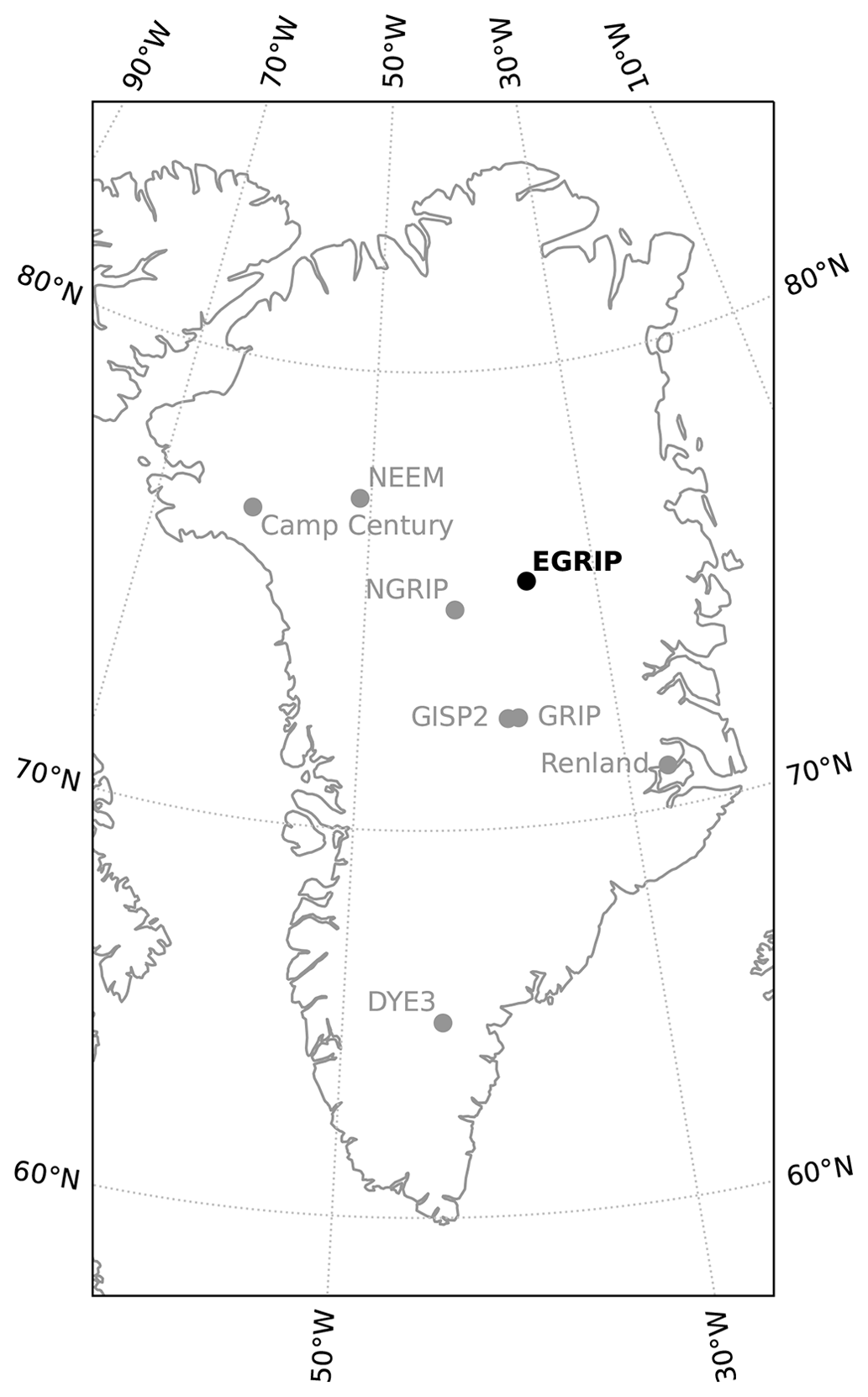
Figure 1Coring location of the EGRIP ice core in bold with other major ice-core drilling sites in Greenland.
For the continuous flow analysis measurements, samples with a cross section of 36 mm by 36 mm and a length of 0.55m were melted on a gold-plated melthead and only the innermost 26 mm by 26 mm area was used to supply the clean meltwater stream (Bigler et al., 2011). The measurements of the data down to 479 m depth presented here were performed in two melting campaigns in 2018 and 2019 covering the depth range of 13.75–350.35 and 350.35–904.75 m, respectively. The samples for the measurements down to 350.35 m were cut entirely in the field, and 0.55 m pieces were then shipped via Copenhagen to Bern for analysis. Below that, the chemistry CFA sticks and the neighboring gas CFA sticks were not split in the field but were shipped as 36 mm by 72 mm by 0.55 m slabs to Copenhagen, where they were split prior to the shipment to Bern. This was done to guarantee higher sample quality for the CFA measurements in the brittle-ice section of the core, starting below the depth section presented here.
All measurements were performed at the continuous flow analysis lab at the University of Bern instead of in the field as had been the case for the NGRIP (North Greenland Ice Core Project) and NEEM (North Greenland Eemian Ice drilling, Dahl-Jensen et al. (2002)) deep-drilling campaigns in Greenland. This change was necessary due to the addition of an ICP-TOFMS to the setup that is not easily field-deployable. In the CFA lab, the melthead is located in a −20 ∘C cold cell that is also used to prepare the samples for the measurements. The meltwater is pumped to the warm part of the lab for subsequent analysis.
For the EGRIP measurement campaigns, the analytical methods of the Bern CFA system were used basically unchanged from the NEEM system (Kaufmann et al., 2008; Erhardt et al., 2022a) with the exception of some changes to the melting procedures and the addition of a directly coupled ICP-TOFMS (icpTOF R, TOFWERK, Thun, Switzerland) (Erhardt et al., 2019). The addition of an ICP-TOFMS constitutes the largest change to the previously described system and will be outlined separately in Sect. 4.2.
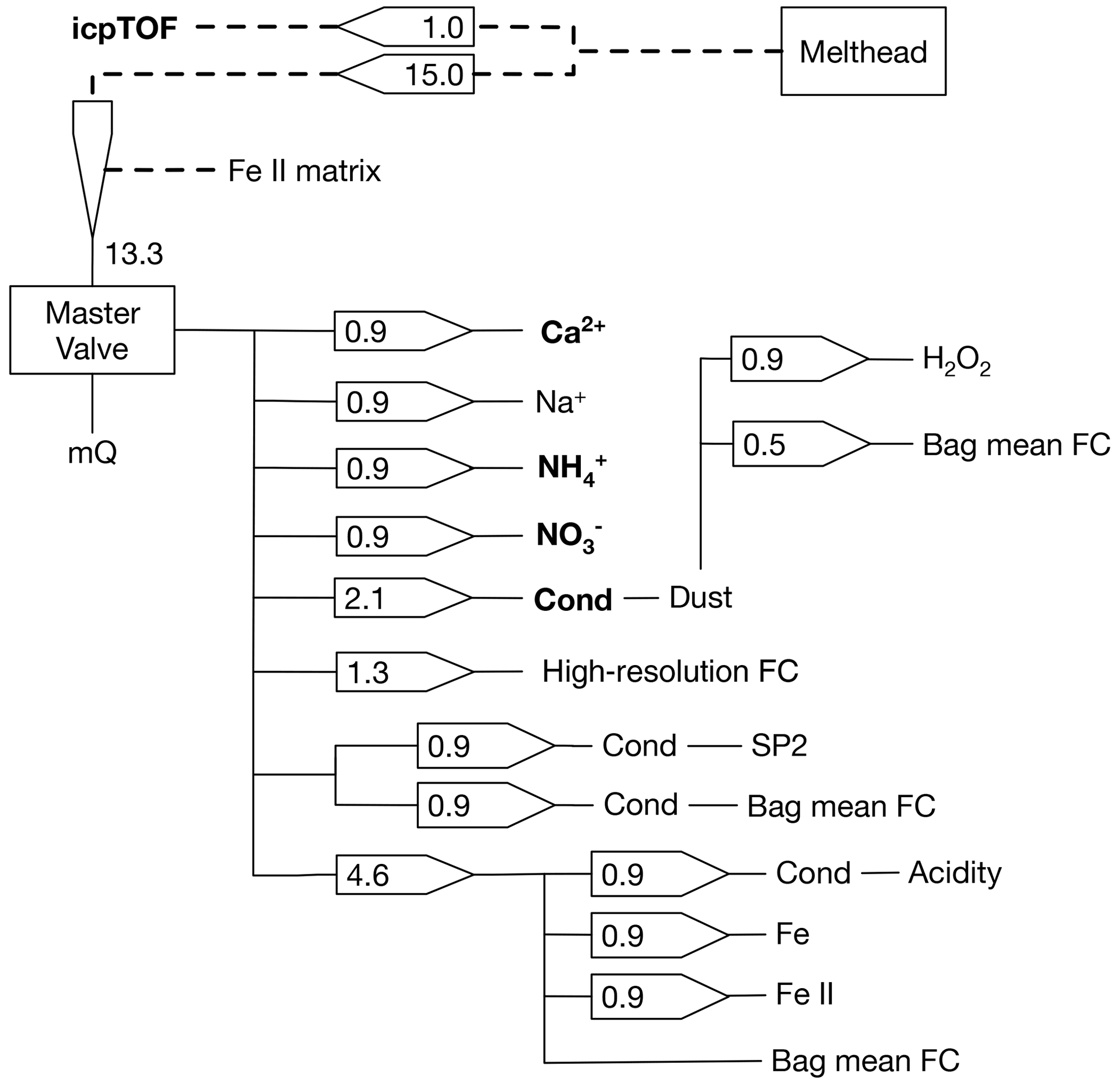
Figure 2Water flow distribution from the central part of the melthead between all channels in the EGRIP CFA setup used for the top 350 m of the core in the 2018 melt campaign. Not shown is the meltwater stream from the outside the core sample that was collected for cosmogenic radionuclide measurements. All arrows denote peristaltic pump channels with pump rates given in mL min−1. Dashed connections denote mixed air–water streams and solid lines pure water streams. Bold labels indicate channels used for the data presented here. “Bag mean FC” denotes fraction collection (FC) at 0.55 m resolution.
In addition to the measurements described here, the CFA system supplied clean meltwater streams to additional analysis channels and sampling efforts. The complete distribution of the meltwater streams between the different analysis channels of the Bern system and the measurements of the sampling efforts of the partner institutes for the 2018 melting campaign are shown in Fig. 2. These were set up and run in Bern by the international partners in the EGRIP project and include the continuous analysis of dissolved iron (Fe) and Fe II (Burgay et al., 2018, run by the University of Venice, Italy) and black carbon using an SP2 instrument (Mori et al., 2016, run by the National Institute for Polar Research, Japan) and an absorption spectroscopic measurement of the meltwater acidity (Kjær et al., 2016, run by the Center for Ice and Climate, Copenhagen, Denmark). The acidity measurements were integrated into the Bern CFA system in 2019 (for data starting from 350.35 m) using a purpose-built spectrometer similar to the ones used for all other channels in the Bern system. Furthermore, samples at 5 and 2.5 cm depth resolution for ion chromatography (run by the Alfred Wegener Institute, Bremerhaven, Germany) as well as multiple aliquots at 55 cm resolution were collected for various offline measurements run by the international partners. Finally, excess meltwater from the outer part of the ice stick was collected in 50 ml aliquots for high-resolution measurements of cosmogenic 10Be and 36Cl (Paleari et al., 2022a, b).
4.1 Wet-chemistry measurements
In the following section we provide the main references that describe the system and refer the reader to Erhardt et al. (2022a) for a more detailed discussion of the system and its development over the years. The wet-chemistry (or main Bern CFA) system uses a range of analyte specific absorption and fluorescence spectroscopy methods to measure the low concentration of dissolved Ca2+ (Tsien et al., 1982), Na+ (Quiles et al., 1993), (Genfa and Dasgupta, 1989), (McCormack et al., 1994), and H2O2(Dasgupta and Hwang, 1985) (hydrogen peroxide) in the ice. All of these methods were specifically adapted for the CFA ice-core measurements (Sigg et al., 1994; Röthlisberger et al., 2000; Kaufmann et al., 2008) and employ custom-built spectrometers as described in detail in (Kaufmann et al., 2008). Furthermore, the system employs a conductivity cell (Amber Science) to determine the electrolytic meltwater conductivity (Cond.) and a laser attenuation particle counter and sizer (Abalus, Klotz GmbH) for insoluble particle measurements. In 2019 (starting from 350.35 m) the absorption spectroscopic Na+ measurement was dropped in favor of the more reliable and higher-resolution measurement by the ICP-TOFMS, introduced prior to the 2018 melting and discussed below (Erhardt et al., 2019). Furthermore, H2O2 measurements were halted after the 2018 season because of the loss of a useful signal due to excessive diffusion. Here we only provide data of Ca2+, , and concentrations and electrolytic meltwater conductivity from the wet-chemistry CFA.
4.2 Continuous ICP-TOFMS
The addition of an inductively coupled plasma time-of-flight mass spectrometer (ICP-TOFMS) is the biggest analytical change in the Bern CFA system in comparison to previous melting campaigns. The coupling and integration of the ICP-TOFMS to the Bern CFA setup and the instrument parameters have been described in detail in Erhardt et al. (2019) and will only be outlined briefly in the following. The main feature of the icpTOF is the fact that the time-of-flight mass spectrometer can measure the complete mass range of 23 to 275 at a sampling rate of 33 kHz allowing the temporal resolution of short transient signals and coverage of almost the entire table of elements. For the CFA analysis, the instrument is run in two different data acquisition modes: either at an integration time of 250 ms for normal data acquisition of total elemental concentrations or at 2 ms integration time to also resolve the ionization events of individual particles entering the plasma in the single-particle mode.
The sample stream for the ICP-TOFMS is diverted close to the melthead from the main meltwater stream. The air–water mixture coming from the melthead is used to efficiently transport particulates to the instrument and to limit signal dispersion. The air is released from the ice during melting and thus does not pose a contamination risk as would other external gas sources. The air is only removed very close to the instrument using a custom build Teflon micro-volume debubbler with a volume of approximately 100 µL. The bubble-free sample stream is then slightly acidified to 1 % using high-purity nitric acid (Optima Grade, Fisher Scientific) close to the sample introduction of the instrument. In this way washout times from the nebulizer and spray chamber can be minimized without risking the dissolution of particles in the ice which are the focus of the single-particle measurements. During the acidification, Rh (rhodium) is added to the sample as an internal standard to monitor system stability and correct for sensitivity drifts. The sample is introduced into the plasma via a quartz cyclonic spray chamber at a flow rate of 400 µL min−1 using a glass concentric nebulizer (Micro Mist, Glass Expansion) for the 2018 melting campaign (to 350 m depth) and a Teflon nebulizer (MicroFlow PFA-ST, Elemental Scientfic) thereafter. Detailed information on plasma conditions used for both cases can be found in Erhardt et al. (2019).
Before and after each measurement run the instrument is calibrated with a range of multi-element standards. All standards are prepared by gravimetrically mixing multi-element standards (Sigma Aldrich, Inorganic Ventures) for a stock solution, which is then further diluted into working standards that span the expected range of concentrations in the ice. Due to the wide mass range that is covered by the TOFMS and the fact that mass-scanning is now necessary to acquire different masses, the range of analytes that can be targeted is basically only limited by their calibration and their possible interference. Even though the data presented here only contain Na and Ca concentrations, the instrument is routinely calibrated for a wide range of analytes including halogens, rare-earth elements, and heavy metals and platinum group elements. These data are still under evaluation and are not provided here. For the calibration measurements an SC-µDX autosampler with FAST injection valve (Elemental Scientific) was used to allow for repeatable and time-efficient calibrations. Measurements were performed by injection of a 400 µL loop into a dilute nitric-acid carrier stream which was run continuously between measurement runs.
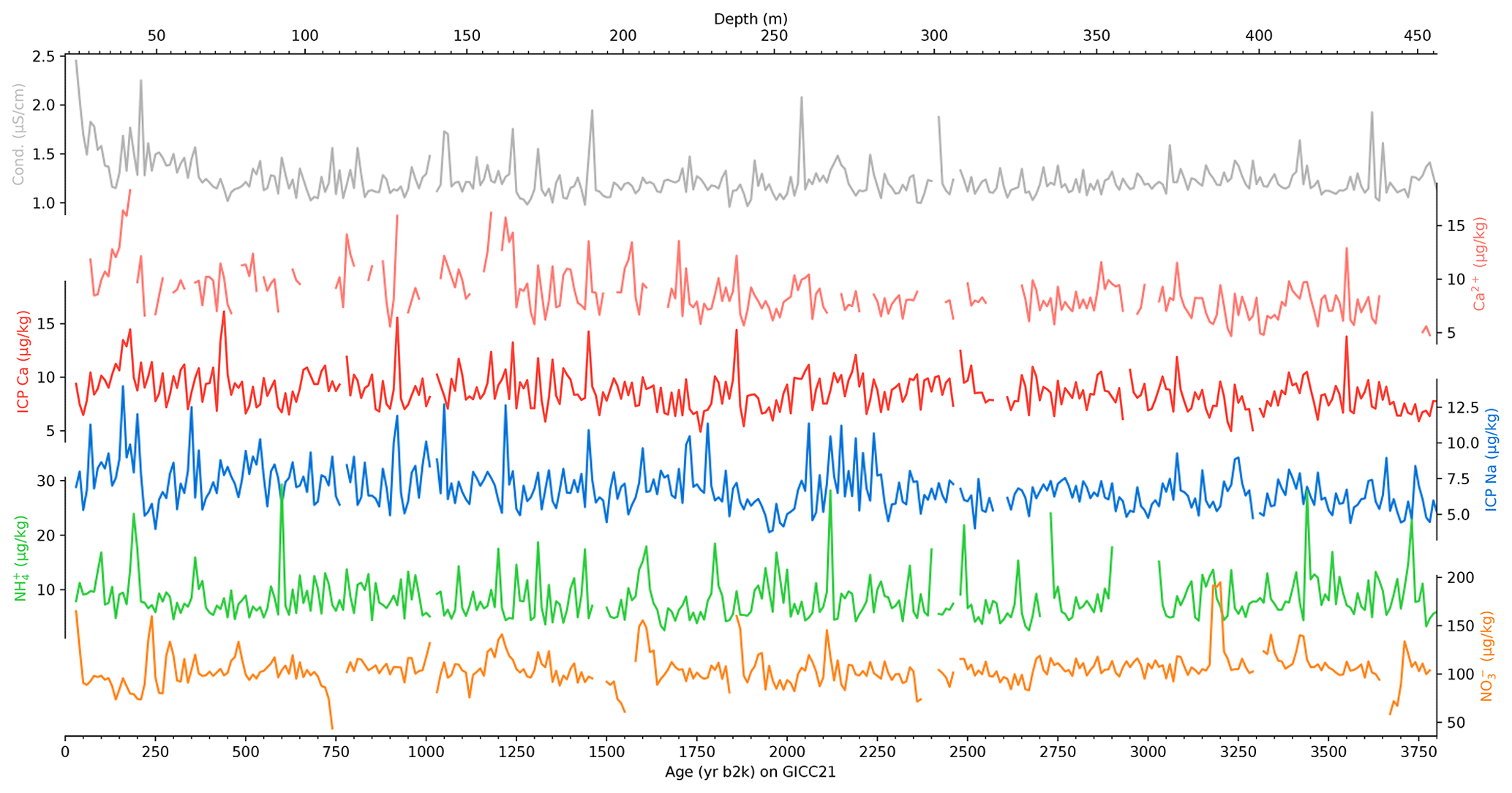
Figure 3Overview of the complete data set at 10-year resolution on the GICC21 (Sinnl et al., 2022) age scale. From top to bottom the data series are electrolytic meltwater conductivity (Cond.), Ca2+ measured by fluorescence spectrometry, Ca and Na measured by ICP-TOFMS, measured by fluorescence spectrometry, and measured by absorption spectrometry. Note that the Ca2+ record partly suffers from analytical issues leading to a large number of gaps in the final data set. However, the Ca data from the ICP-TOFMS cover most of these gaps and provide an almost complete data set.
For the data presented in this study, both normal (4 Hz) and single-particle (500 Hz) acquisition data were averaged to the nominal 1 mm resolution used for all of the data series from the main CFA system. The final data set is then smoothed with a 10 s cutoff frequency Gaussian filter to remove high-frequency measurement noise from the data set. The depth assignment of the ICP-TOFMS data was achieved by aligning the Ca data to the raw fluorimetric Ca2+ measurements of the main CFA system and thus to its depth scale.
Figure 3 shows an overview of all data sets provided here at a 10-year resolution on the GICC21 (Sinnl et al., 2022) age scale, both from the wet-chemistry CFA as well as from the ICP-TOFMS. Note that even though the final data set of Ca2+ exhibits large gaps, the depth assignment of the ICP-TOFMS Ca data set is done using the raw fluorescence intensity data, as elaborated above. Thus the depth assignment of the Ca data is well constrained even when calibration issues affect the Ca2+ data as described in Sect. 5.1.
4.3 Updated melting and measurement procedure
Previously, the Bern CFA system was run with 1.10 to 1.65 m of ice per run at most (Erhardt et al., 2022a), i.e., two to three times 0.55 m per continuous measurement run. This maximum length is dictated by the length of the frames used to guide the ice during melting and by the vertical space available for the melting unit. Between each of the measurement runs, all connected instruments are run on an ultrapure water stream. Depending on the method it can take a significant time to reach a stable baseline signal between the runs, which is needed to catch and correct for drift in the analysis units. In a typical campaign, two to three runs were performed before a calibration run approximately every 2 to 3 h, which means that the waiting time between each run adds up to a large fraction of each measurement day.
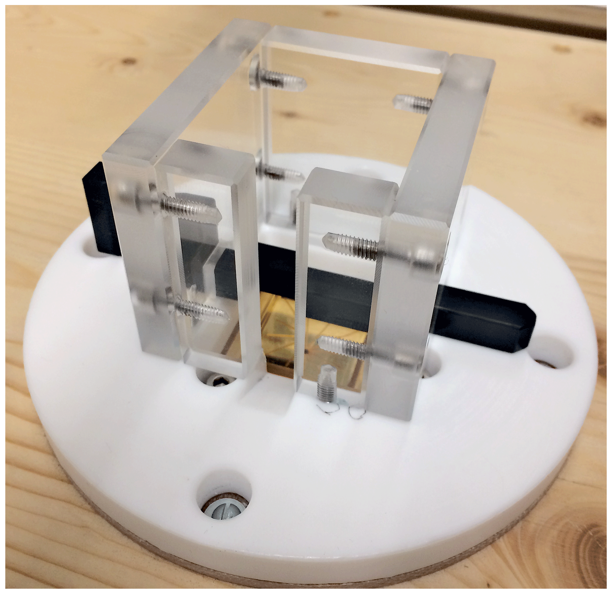
Figure 4Picture of the melthead and the additional transparent sample guide used for the stacking of core segments during melting.
To capitalize on the stability of the well-matured Bern CFA system and the environmentally more stable lab setting as compared to the field, the melting procedure for the EGRIP ice core was changed to allow the uninterrupted measurement of multiple frames worth of ice-core samples by exchanging the frames mid-run. This is achieved by adding an additional fixed sample guide shown in Fig. 4 to the Teflon melthead cover similar to what is also done in other CFA labs. During a measurement run, the frames can then be exchanged as soon as there is only so much ice left on the melthead (∼10 cm) that it reaches the top of the new sample guide. To do so, the weight connected to the depth encoder of the CFA system is lifted from the remaining ice, the empty frame is removed from the holder, and a new one is put in its place. The new piece of ice is then lowered carefully down to the remainder on the melthead using a Teflon wedge. Finally the encoder weight is then placed on top of the new sample. After some training, the whole procedure can be done within a few seconds, during which the melting of the small remainder of ice continues. In this time a little less meltwater is produced; however, the amount is still enough to avoid contamination by inflow from meltwater from the outside of the sample. During the procedure no depth recording is possible; however, due to the short amount of time needed to re-position the encoder on the new piece of ice only very little ice melts during this time, as discussed below. The total amount of ice that can be measured in each measurement run is limited by the system stability and the frequency of calibration runs between extended ice measurements.
For the data presented here, usually a total of 3.30 m of ice were melted within each run, amounting to approximately 2 h of uninterrupted measurement time per run at a melt speed of 2.7 cm min−1. During each measurement day, a total of four runs with bracketing calibrations were performed. Depending on sample quality, this amounts to a total daily production of approximately 12–14 m per ∼16 h workday including the daily startup and shutdown of all instruments.
The discussion of the uncertainties is split into three major parts: the analytical precision of the measurements, the depth assignment, and the resulting depth and temporal resolution. To complete the discussion we added a few notes on the effect of the melt speed stability on the data resolution as well as a brief comparison to calcium data sets.
5.1 Analytical precision
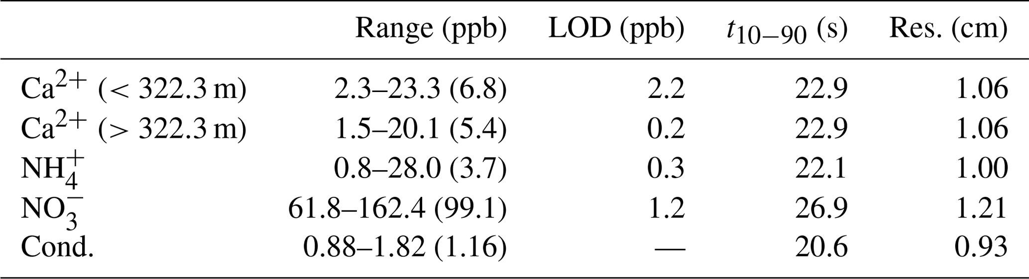
Because the spectroscopic methods used here were essentially not modified since the last measurement campaign (i.e., NEEM), the detection limits and uncertainties are assumed to have remained largely unchanged. The relevant numbers for each of the detection channels are listed in Table 1. As discussed in Gfeller et al. (2014), the uncertainty in the wet chemistry is dominated by the uncertainty of the standard preparation by use of the water dispenser and microliter pipette. For the concentration ranges discussed here, these uncertainties typically amount to less then 10 %. For the wet-chemistry CFA data, the limit of detection (LOD) was determined as 3 times the standard deviation of the baseline/blank signal from ultrapure water (mQ, Merck/Millipore). In the case of the Ca2+ data, an issue with the fluorescence detector caused a low sensitivity in the top 322.3 m of the data set, leading to a much higher limit of detection in this section of the core as indicated by the two different values in Table 1. The lower sensitivity and the resulting higher limit of detection also affects the Ca2+ concentration range for the upper part of the core as values below the LOD were removed from the data.
Table 1Analytical figures of merit for the wet-chemistry data. The sample concentration ranges are given by the 5th and 95th percentile and the median value in parentheses. The limit of detection is calculated as 3 times the standard deviation of the blank signal. The temporal resolution of the detection channels is determined as the long-term average 10 %–90 % rise time, which is converted to an equivalent depth resolution assuming a melt speed of 2.7 cm min−1. Note that this resolution does not account for signal dispersion during melting and in the debubbler.
For the ICP-TOFMS measurements of Ca and Na, the relevant performance numbers are given in Table 2. Here the values include the relative uncertainties from the standard errors of the calibrations. In the case of the ICP-TOFMS data, LODs were determined using 3 times the standard error of the regression for the calibrations. These regressions include the blank measurements and allow for a non-zero intercept. This approach was chosen as it yielded more reliable results and allows for the determination of the LODs even in the occasional case if no reliable blank measurement could be performed.
Table 2Analytical figures of merit for the ICP-TOFMS data. The sample concentration ranges are given by the 5th and 95th percentile and the median value in parentheses. The relative uncertainty (Rel. Uncert.) values are given for the respective concentrations in the range column. The limit of detection is determined from 3 times the standard error of the regression line at its intercept. The temporal resolution of the detection channels is determined as the long-term average 10 %–90 % rise time, which is converted to an equivalent depth resolution assuming a melt speed of 2.7 cm min−1. Note that this resolution does not account for signal dispersion during melting and in the debubbler.
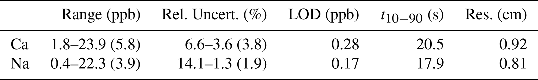
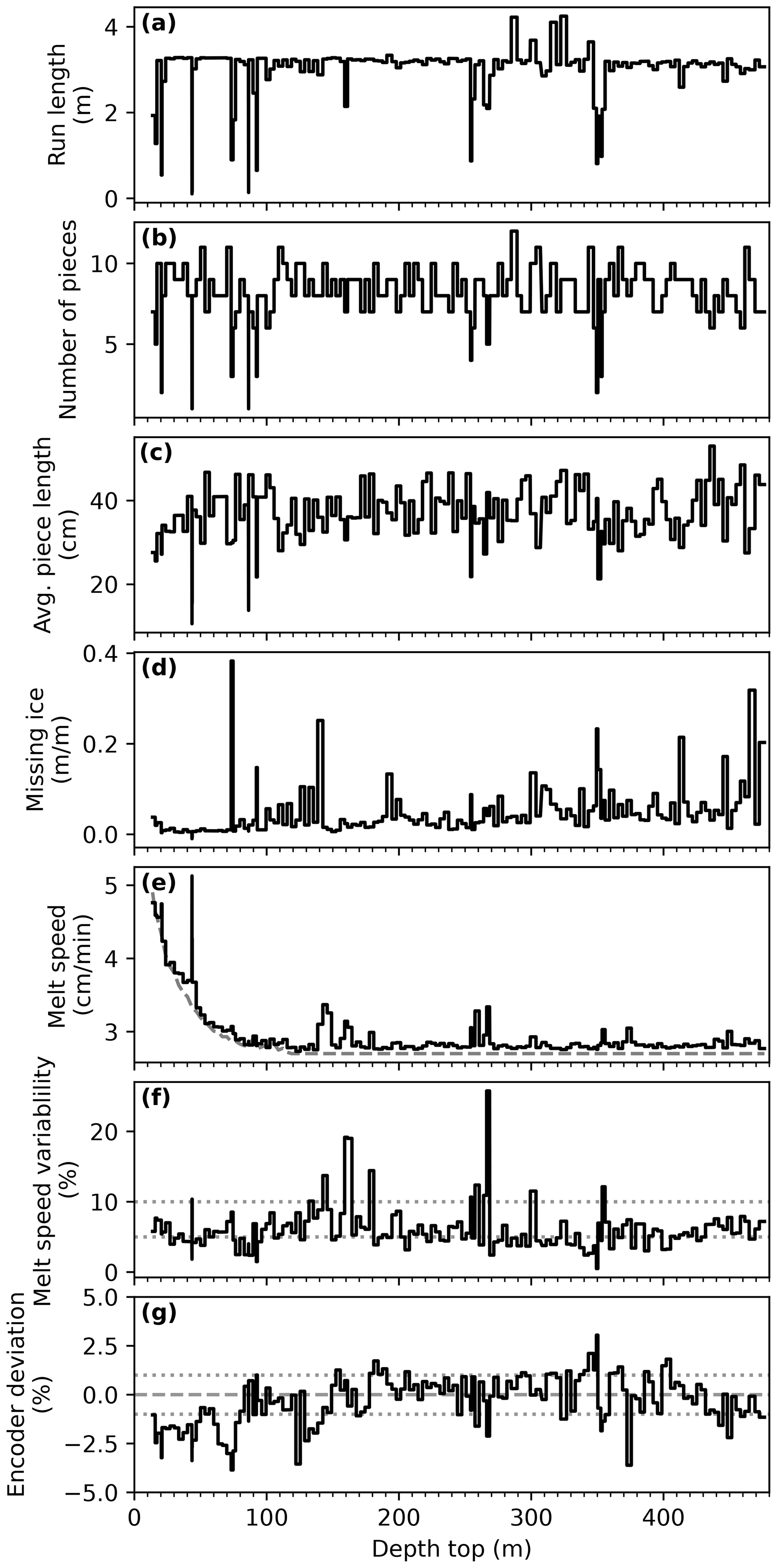
Figure 5Depth assignment statistics. Panels (a)–(d) show information on the amount of ice melted during each run (a) and the number of pieces of ice (b), their average length, and the amount of ice that is missing as indicators for the sample quality. Panels (e)–(g) show the melt speed (e) alongside the target melt speed of 2.7 cm min−1 in ice equivalent, the inter-run variability of the melt speed (f) as an indicator for the melt speed stability, and the encoder deviation (g) as an indicator of the depth-assignment precision. In panel (f), the horizontal lines mark 5 % and 10 % variability and in panel (g) 0 % and ±1 % deviation.
5.2 Depth assignment
Previous investigations (Röthlisberger et al., 2000; Hiscock et al., 2013) have reported the uncertainty of the depth assignment of the 110–165 cm measurements runs as ±1 cm. The total precision of the depth assignment is likely limited by the precision of the length measurements during sample preparation due to the possible influence of parallax effects and the limited precision of rulers (Erhardt et al., 2022a). However, due to the aforementioned change in the melt protocol in comparison to previous studies, the quality of the depth assignment merits some additional discussion below. Overall, the uncertainty of the absolute depth assignment of all records to the ice-core depth is about 2 cm, while the offsets between the individual CFA records are only on the order of 1 mm.
As mentioned above, during the stacking, the weight that is connected to the depth encoder of the CFA system is lifted from the ice. During that time, the remaining ∼10 cm of ice continue to melt, albeit slower than usual, due to the missing pressure from the encoder weight. Due to the encoder being removed during that time, usually for around 5–15 s, the progress of the melting is unrecorded. The resulting gaps in the depth assignment are filled during the data processing using linear interpolation. Furthermore, because the amount of ice is greater per run than previously, the total amount of ice contains more breaks adding to the depth-assignment uncertainty. This is due to the fact that each break surface will need to be cleaned and squared, each of which carries the risk of mis-measurement of the total length of ice.
To investigate the influence of the stacking procedure on the depth-assignment uncertainty, we look at the discrepancy between the length of ice as measured by the encoder and the length of ice measured during sample preparation, shown as relative deviation in Fig. 5g. Comparing the deviations to the length statistics shown in Fig. 5a–c, most notably, the relative deviation between melted and measured sample lengths for the runs does not show any correlation with the total amount of ice melted or the number of pieces that make up the total length of the ice. This indicates that the stacking procedure does not introduce excessive additional uncertainty.
In the shallow part of the ice core, down to approximately 100 m depth where the melt speed is higher than 2.7 cm min−1, the melted length of ice is systematically lower than the amount measured before the melting. We suggest that this can be attributed to a slight compaction of the fragile firn during sample handling and the upright melting due to the overburden of the sample and the encoder weight.
The deviation between the two length measurements can also be used to estimate the overall uncertainty of the depth assignment. On average, if the measurements are not biased and their errors are not correlated, the difference between them should be zero, and its variance is the sum of the variances of the two measurements, providing the overall squared uncertainty of the depth measurement. To provide an average uncertainty we report half the overall relative standard deviation of the difference between the known encoder calibration (cm−1) and the observed number of encoder counts per centimeter of ice melted as the upper estimate of the depth assignment uncertainty. In this way the provided uncertainty is independent from the exact amount of melted ice. Furthermore, the beginning and the end of the run are used as reference points to fix the length of ice measured on the overall depth scale of the ice core. That means that the error in the depth assignment relative to the ice-core depth scale is by definition zero at these points, further reducing the overall uncertainty. In the shallow part of the data, as mentioned above, one of the measurements is biased and the aforementioned assumption not valid. Excluding measurements above 100 m depth, the relative uncertainty in the depth assignment is 0.54 %, amounting to 1.8 cm for a 3.3 m run. Over the complete depth range of the data here the same calculation yields 0.64 % or 2.1 cm for a 3.3 m run.
Overall, we judge the relative uncertainty of the depth assignment not to be affected by the core-stacking process beyond the approximately 1 % of the amount of ice melted per measurement as previously reported for solid ice (Erhardt et al., 2022a). As discussed in Erhardt et al. (2022a) this uncertainty mainly arises from the sample preparation and the melting procedure itself only contributes a small part of the overall uncertainty. We note that the overall uncertainty can further be reduced by incorporating the 55 cm bag marker into the depth assignment procedure.
It is worth noting, however, that these sources of uncertainty for the absolute depth assignment do not contribute to the phasing error between the different analytes. The relative alignment between the parameters of the main CFA system is performed as described previously using short injections of a multi-component standard to determine the delays to each of the wet-chemistry channels. As discussed in Erhardt et al. (2022a), the uncertainty of this relative phasing is on the order of 1–2 s, translating to less than a millimeter at the melt speeds employed here. The relative alignment of the ICP-TOFMS data is performed by alignment of the Ca to the Ca2+, transferring the relative phasing uncertainty of the wet-chemistry CFA to the ICP-TOFMS measurements (Erhardt et al., 2019). In summary, while the uncertainty in absolute depth of all records may be about 2 cm, the relative depth offsets between individual CFA records is only on the order of 1 mm.
5.3 Depth and temporal resolution
The resolution for both the wet-chemistry CFA data sets as well as the ICP-TOFMS was determined by the 10 %–90 % rise time of standard measurements, treated in the same way as the sample measurements with respect to temporal resolution and smoothing of the raw signals. Overall, the resolution of the data is on the order of approximately 1 cm as listed in Tables 1 and 2. The data, due to the long tubing and the reaction column involved, exhibit a slightly lower resolution at 1.2 cm. Both the electrolytic meltwater conductivity and the ICP-TOFMS measurements have slightly better resolution, below 1 cm. Note that these values do not include the additional dispersion that happens during melting and in the de-bubbling volumes. However, as argued before (Erhardt et al., 2022a; Sigg et al., 1994), the response time of the detection usually dominates the overall signal dispersion, and the numbers reported can serve as a good guidance for the overall resolution of the data. Generally, the resolution of the CFA-ICP-TOFMS data is slightly better than that of the corresponding wet-chemistry measurement including the dispersion during the melting and in the respective debubbler volumes, as a direct comparison of the high-frequency content of a section of the data has shown (Erhardt et al., 2019).
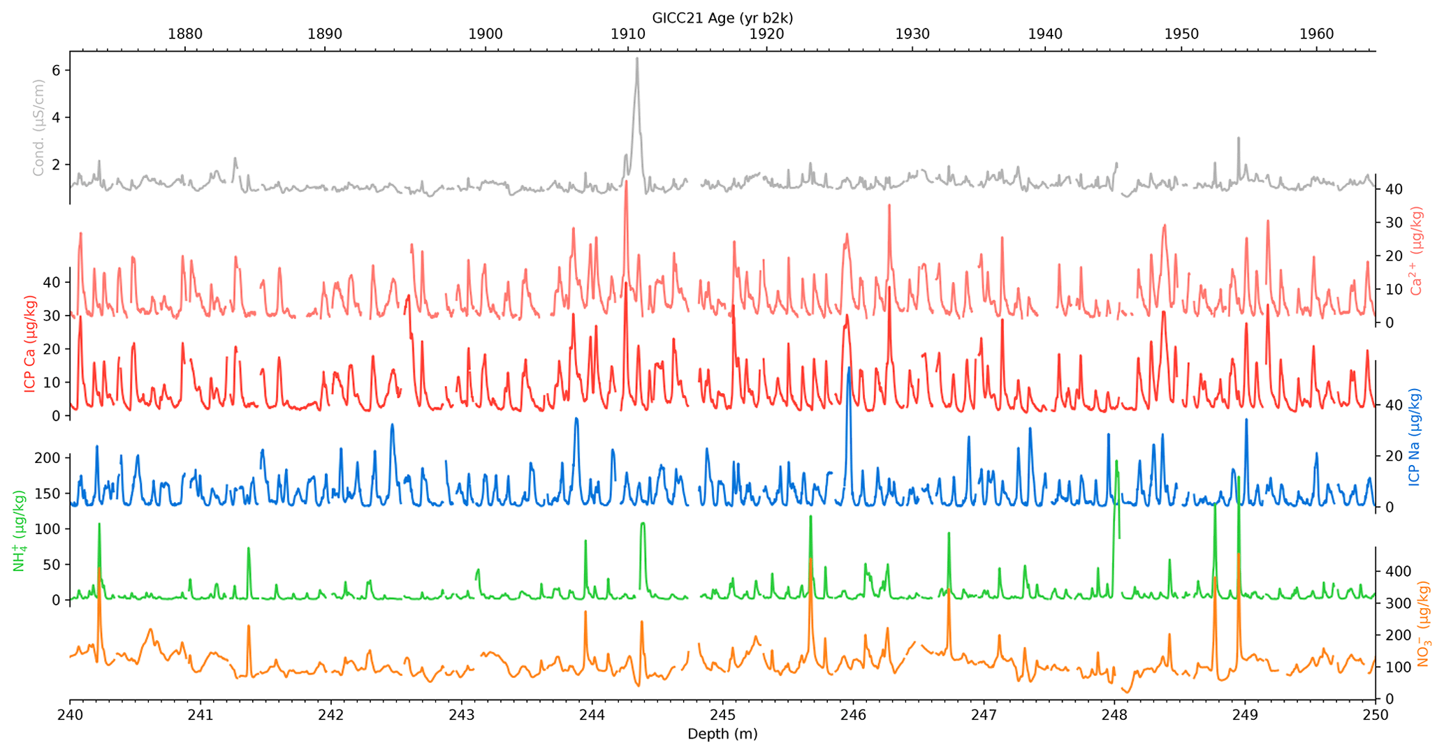
Figure 6Example of high-resolution data over a 10 m section of the core. The parameters shown are the same as in Fig. 3; however, data are shown on the depth scale, with the secondary x axis at the top indicating the age at annual resolution. The large peak in conductivity at 244.3 m is a typical signal of a volcanic eruption and has been used to synchronize the age scales between different ice cores.
Figure 6 shows a 10 m section of the data at the full nominal 1 mm resolution. This example shows the very clear resolution of the seasonal variability in all of the parameters as exploited in the revision of the GICC (Greenland Ice Core Chronology) timescale (Sinnl et al., 2022). The peak dominating the electrolytic meltwater conductivity record in Fig. 6 is a typical signal from aerosol deposition after a volcanic eruption. This specific eruption signal has previously been attributed to the 79 CE Vesuvius eruption, which has recently been ruled out by tephra evidence pointing to a source in the Aleutian Arc (Plunkett et al., 2022). In correspondence with other dating efforts (e.g., Sigl et al., 2015), the eruption is now dated to 87/88 CE on the GICC21 age scale (Sinnl et al., 2022).
For the depth resolution, the melt speed and its stability play an important role in determining the overall resolution as well as the stability of this resolution. Especially in the shallow parts of the core, above the depth when the firn reaches the density of ice at 917 kg m−3, this is an important factor. For technical reasons, i.e., to supply enough meltwater for the system, the melt speed above the firn–ice transition needs to be increased to match the melt speed in ice-equivalent depth. This is clearly visible in Fig. 5e, with the exponential decrease in the melt speed for the top ∼100 m of the core. Through the adjustment of the melt speed, the data which are measured at constant time intervals, are measured at a constant resolution in terms of the ice-equivalent depth. Assuming an approximate constant annual layer thickness, this translates to an approximate constant temporal resolution as well. Figure 5f shows the variability of the melt speed within each of the measurement runs. This is a measure of how constant the resolution of the data is. High melt speed variability will translate directly into variability of the measurement resolution in terms of depth along the core. Overall, this variability given by the relative standard deviation is significantly lower than 10 %, and mostly around 5 %. Runs with much higher variability are usually caused by sample quality issues which resulted in interrupted melting. In some cases such variability can be caused by too-thin ice sections that were intentionally melted faster to avoid contamination by the intrusion of meltwater from the outside the melthead to the clean part inside. However, because of the mixing in the system and because of the response time of the detection method on the order of ∼20 s, any short-term variability likely plays a minor role in terms of jitter or the determination of annual layer thicknesses from the data.
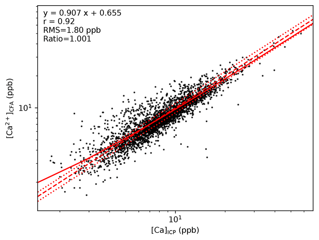
Figure 7Cross plot of ICP-TOFMS Ca and fluorimetric Ca2+ concentrations at 10 cm resolution, considering only sections with less than 50 % missing data. Regression, Pearson correlation (r), root mean square error (rms), and the average ratio were calculated on the concentrations (i.e., not log-transformed). The solid line is the result of the regression, the dashed line marks the 1:1 line, and the dotted lines indicate a ±10 % deviation from that line.
5.4 Ca records
Because the Ca and Ca2+ concentrations were measured using two different and entirely independently calibrated methods, they allow for direct comparison between the fluorimetric detection and ICP-TOFMS measurements at high resolution. Figure 7 shows a direct comparison of the records at 10 cm resolution alongside a linear regression between the two, their correlation, root mean square (rms) difference, and average ratio. Generally both data sets agree very well with each other despite the differences in measurement techniques as indicated by the low rms difference, high correlation, and close-to-unity average ratio. The linear regression between the two indicates a small constant offset between the two. This is likely caused by the aforementioned Ca2+ sensitivity and LOD issues in the top part of the data set as the offset vanishes when looking only at data below 322.3 m. However, measurements below the baseline for Ca2+ were removed from the data set and the apparent offset is small in comparison to the concentrations and their uncertainties.
At a higher resolution, as illustrated in Fig. 6, the agreement between the two measurements is also very good. Focusing on 1 m sections of the full resolution 1 mm data, the average correlation between the two measurements is 0.95 with an rms difference of 2.44 ppb.
In summary, the agreement both at low and high resolution between the two data sets illustrates their compatibility as well as their high quality. However, it is worth noting that it is not given a priori that the two should agree as they fundamentally measure two different things. Ca2+ in the meltwater steam is the result of water-soluble calcium species that are dissolved during the melting and transport of the sample. These are only a subset of the total amount of Ca that is present in the meltwater, which is what the ICP-TOFMS measures. For example, in case of the presence of a high load of poorly soluble Ca-bearing mineral dust particles in the ice, the ICP-TOFMS will detect significantly more Ca than the fluorimetric Ca2+ measurement. That being said, the close agreement between the two suggests that most of the total Ca present in the ice is soluble in the meltwater stream. A detailed comparison of the differences between the two and how they arise is planned.
For the drilling of the EGRIP ice core the same drill liquid combination of COASOAL and ESTISOL 240 (Popp et al., 2014) was used as for the NEEM ice core. The drill liquid acts as an absorber of bivalent cations in the CFA system if it is introduced by contaminated ice. This can have a detrimental effect on the measurement of Ca2+ and likely all other bivalent cations by producing strong absorption/desorption signals during measurement runs (Erhardt et al., 2022a). As almost all of the calcium detected by the ICP-TOFMS is also dissolved Ca2+, the same is true for the total Ca measurements. To counteract the risk of drill liquid entering the melt system, special care was taken during sample preparation to remove all possibly contaminated ice either by scraping off or cutting out possibly affected ice. This is especially important for small, refrozen, and often hard to see cracks in the sample. For the data presented here, this effort, possibly in combination with the low Ca concentrations in the Holocene ice, has proven to be very fruitful. The data were found to be free of the previously described absorption/desorption effects, and no correction was necessary.
As mentioned above, the EGRIP ice core is located inside the Northeast Greenland Ice Stream, and at the coring location surface velocities are 55 m a−1 (Hvidberg et al., 2020), and ice down-core originates from a location closer to the ice divide, likely characterized by a higher accumulation rate (Gerber et al., 2021). This change in location and especially in the accumulation rate of about ∼30 % likely also has an influence on the aerosol data presented here both due to the change in deposition characteristics as well as due to the change in distance from possible source areas (e.g., Fischer et al., 1998a, b). Furthermore, short-term variability in the data sets is likely affected by the varying influence of the local topography changes upstream (e.g., Winski et al., 2019), leading for example to accumulation variability independent of precipitation on length scales of meters (sastrugi) to kilometers (dunes) due to wind reworking. That means that both long-term trends as well as short-term variability in the data will need to be interpreted with great care and in the light of the influence of the upstream effects.
Both the full 1 mm resolution as well as the decadally averaged data are available on PANGAEA under a CC-BY license (https://doi.org/10.1594/PANGAEA.945293 Erhardt et al., 2022b):
-
full resolution – https://doi.org/10.1594/PANGAEA.945290 (Erhardt et al., 2022c);
-
decadal averages on the GICC21 age scale – https://doi.org/10.1594/PANGAEA.945291 (Erhardt et al., 2022d).
The GICC21 age scale can be found in the supplement of Sinnl et al. (2022).
Here we present a multi-proxy record of impurity concentrations from the EGRIP ice core covering the past 3.8 kyr. The data were measured using the state-of-the-art continuous flow analysis system at the University of Bern and include measurements of dissolved calcium, ammonium, and nitrate from spectrophotometric measurements, electrolytic meltwater conductivity, and total calcium and sodium concentrations measured by online ICP-TOFMS. The high-resolution records presented have sub-annual resolution and have formed part of the database for the revised Greenland ice-core chronology, the GICC21, over the past 3.8 kyr (Sinnl et al., 2022).
Summarizing from the previous section we stress the following points that should be considered when using these data:
-
The data sets have undergone extensive quality control both manually and automated. However, we cannot guarantee the complete absence of any spurious signals, especially at the full resolution.
-
Similar to previous CFA data sets, the depth assignment to a given down-core depth is likely accurate to better than 2 cm. The relative depth assignment within the CFA data set is much more accurate and uncertainties are on the order of 1 mm.
-
Analytical uncertainties for the wet-chemistry data (Ca2+, , ) are typically better than 10 % and for the ICP-TOFMS data (Ca, Na) better than 5 %.
-
The fluorescence spectrometric Ca2+ data above 322.3 m depth suffer from decreased sensitivity of the measurement setup and have higher-than-usual limits of detection. Values below the baseline were removed from the data set.
-
All the aerosol concentrations in the EGRIP ice core, including the ones presented here, are likely affected by upstream effects due to changes in the local deposition regime and distance from the aerosol source regions further upstream. These effects are subject to ongoing investigation, and they need to be taken into account when interpreting the data at any temporal scale.
-
Last but not least, we stress that any detailed interpretation, especially of short-term signals in the data sets should always be confirmed at least within the multi-parameter data series, if not with additional data or measurements.
We invite any future user of these data sets to actively involve CFA or ice-core specialists in their investigation for an expert assessment of the data quality and limitations, which may be specific to the application intended by the data user in order to avoid any shortcomings and pitfalls of the complex data sets.
The CFA campaigns at the University of Bern were organized and hosted by TE and CMJ under the lead of TE. FA supported the wet-chemistry CFA measurements. The wet-chemistry CFA data were processed and quality controlled by CMJ and the ICP-TOFMS data by TE. TE wrote the initial draft of the paper and prepared the figures. The paper and figures were finalized with input from HF, CMJ, HAK, MB, DS, AS, NM, RM, FB, FA, and IC. All authors took part in the measurement campaigns or contributed to their success.
The contact author has declared that none of the authors has any competing interests.
Publisher's note: Copernicus Publications remains neutral with regard to jurisdictional claims made in the text, published maps, institutional affiliations, or any other geographical representation in this paper. While Copernicus Publications makes every effort to include appropriate place names, the final responsibility lies with the authors.
Purchase of the icpTOF has been made possible through the Swiss National Science Foundation (SNF) R'Equip proposal iceCP-TOF (grant no. 206021_170739) and specific institutional funds made available by the University of Bern. The long-term financial support of ice-core research at the University of Bern by the Swiss National Science Foundation (grant no. 200020_172506 (iCEP) and 20FI21_164190 (EGRIP)) is gratefully acknowledged.
EGRIP is directed and organized by the Centre for Ice and Climate at the Niels Bohr Institute, University of Copenhagen. It is supported by funding agencies and institutions in Denmark (A. P. Møller Foundation, University of Copenhagen), USA (US National Science Foundation, Office of Polar Programs), Germany (Alfred Wegener Institute, Helmholtz Centre for Polar and Marine Research), Japan (National Institute of Polar Research and Arctic Challenge for Sustainability), Norway (University of Bergen and Trond Mohn Foundation), Switzerland (Swiss National Science Foundation), France (French Polar Institute Paul-Emile Victor, Institute for Geosciences and Environmental research), Canada (University of Manitoba), and China (Chinese Academy of Sciences and Beijing Normal University).
Motohiro Hirabayashi, Kaori Fukuda, and Jun Ogata acknowledge financial support by JSPS KAKENHI (grant no. JP18H04140).
The authors gratefully acknowledge the contributions of the countless people that facilitated and took part in the field campaigns and the ice-core drilling and processing and who helped during the CFA melting campaigns.
Furthermore the authors are especially grateful for the help of Priska Lehmann, Sam Black, Patrick Zens, Miriam Läderach, and Michelle Shu-Ting Lee during the campaigns.
We thank the two reviewers for their thoughtful comments and suggestions that improved the paper. We also thank Xingchen Wang for handling the review process as topic editor.
The article processing charges for this open-access publication were covered by the Alfred Wegener Institute, Helmholtz Centre for Polar and Marine Research (AWI).
This paper was edited by Xingchen Wang and reviewed by two anonymous referees.
Bigler, M., Svensson, A., Kettner, E., Vallelonga, P., Nielsen, M. E., and Steffensen, J. P.: Optimization of High-Resolution Continuous Flow Analysis for Transient Climate Signals in Ice Cores, Environ. Sci. Technol., 45, 4483–4489, https://doi.org/10.1021/es200118j, 2011. a
Burgay, F., Erhardt, T., Lunga, D. D., Jensen, C. M., Spolaor, A., Vallelonga, P., Fischer, H., and Barbante, C.: Fe2+ in ice cores as a new potential proxy to detect past volcanic eruptions, Sci. Total Environ., 654, 1110–1117, https://doi.org/10.1016/J.SCITOTENV.2018.11.075, 2018. a
Dahl-Jensen, D., Gundestrup, N. S., Miller, H., Watanabe, O., Johnsen, S. J., Steffensen, J. P., Clausen, H. B., Svensson, A., and Larsen, L. B.: The NorthGRIP deep drilling programme, Ann. Glaciol., 35, 1–4, https://doi.org/10.3189/172756402781817275, 2002. a
Dasgupta, P. K. and Hwang, H.: Application of a nested loop system for the flow injection analysis of trace aqueous peroxides, Anal. Chem., 57, 1009–1012, https://doi.org/10.1021/ac00283a010, 1985. a
Erhardt, T., Jensen, C. M., Borovinskaya, O., and Fischer, H.: Single particle characterization and total elemental concentration measurements in polar ice using CFA-icpTOF, Environ. Sci. Technol., 53, 13275–13283, https://doi.org/10.1021/acs.est.9b03886, 2019. a, b, c, d, e, f, g
Erhardt, T., Bigler, M., Federer, U., Gfeller, G., Leuenberger, D., Stowasser, O., Röthlisberger, R., Schüpbach, S., Ruth, U., Twarloh, B., Wegner, A., Goto-Azuma, K., Kuramoto, T., Kjær, H. A., Vallelonga, P. T., Siggaard-Andersen, M.-L., Hansson, M. E., Benton, A. K., Fleet, L. G., Mulvaney, R., Thomas, E. R., Abram, N., Stocker, T. F., and Fischer, H.: High-resolution aerosol concentration data from the Greenland NorthGRIP and NEEM deep ice cores, Earth Syst. Sci. Data, 14, 1215–1231, https://doi.org/10.5194/essd-14-1215-2022, 2022a. a, b, c, d, e, f, g, h, i, j
Erhardt, T., Jensen, C., and Fischer, H.: High resolution aerosol records over the past 3.8 ka from the EastGRIP ice core, PANGAEA [data set], https://doi.org/10.1594/PANGAEA.945293, 2022b. a, b
Erhardt, T., Jensen, C. M., and Fischer, H.: High resolution aerosol records over the past 3.8 ka from the EastGRIP ice core: 1 mm depth resolution, PANGAEA [data set], https://doi.org/10.1594/PANGAEA.945290, 2022c. a
Erhardt, T., Jensen, C. M., and Fischer, H.: High resolution aerosol records over the past 3.8 ka from the EastGRIP ice core: 10 yr averages on the GICC21 age scale, PANGAEA [data set], https://doi.org/10.1594/PANGAEA.945291, 2022d. a
Fischer, H., Wagenbach, D., and Kipfstuhl, J.: Sulfate and Nitrate Firn Concentrations on the Greenland Ice Sheet. 1. Large-Scale Geographical Deposition Changes, J. Geophys. Res., 103, 1–8, https://doi.org/10.1029/98JD01885, 1998a. a
Fischer, H., Werner, M., Wagenbach, D., Schwager, M., Thorsteinnson, T., Wilhelms, F., Kipfstuhl, J., and Sommer, S.: Little Ice Age clearly recorded in northern Greenland ice cores, Geophys. Res. Lett., 25, 1749–1752, https://doi.org/10.1029/98GL01177, 1998b. a
Genfa, Z. and Dasgupta, P. K.: Fluorometric measurement of aqueous ammonium ion in a flow injection system, Anal. Chem., 61, 408–412, https://doi.org/10.1021/ac00180a006, 1989. a
Gerber, T. A., Hvidberg, C. S., Rasmussen, S. O., Franke, S., Sinnl, G., Grinsted, A., Jansen, D., and Dahl-Jensen, D.: Upstream flow effects revealed in the EastGRIP ice core using Monte Carlo inversion of a two-dimensional ice-flow model, The Cryosphere, 15, 3655–3679, https://doi.org/10.5194/tc-15-3655-2021, 2021. a, b, c
Gfeller, G., Fischer, H., Bigler, M., Schüpbach, S., Leuenberger, D., and Mini, O.: Representativeness and seasonality of major ion records derived from NEEM firn cores, The Cryosphere, 8, 1855–1870, https://doi.org/10.5194/tc-8-1855-2014, 2014. a
Hiscock, W. T., Fischer, H., Bigler, M., Gfeller, G., Leuenberger, D., and Mini, O.: Continuous Flow Analysis of Labile Iron in Ice-Cores, Environ. Sci. Technol., 47, 4416–4425, https://doi.org/10.1021/es3047087, 2013. a
Hvidberg, C. S., Grinsted, A., Dahl-Jensen, D., Khan, S. A., Kusk, A., Andersen, J. K., Neckel, N., Solgaard, A., Karlsson, N. B., Kjær, H. A., and Vallelonga, P.: Surface velocity of the Northeast Greenland Ice Stream (NEGIS): assessment of interior velocities derived from satellite data by GPS, The Cryosphere, 14, 3487–3502, https://doi.org/10.5194/tc-14-3487-2020, 2020. a, b, c
Kaufmann, P. R., Federer, U., Hutterli, M. A., Bigler, M., Schüpbach, S., Ruth, U., Schmitt, J., and Stocker, T. F.: An Improved Continuous Flow Analysis System for High-Resolution Field Measurements on Ice Cores, Environ. Sci. Technol., 42, 8044–8050, https://doi.org/10.1021/es8007722, 2008. a, b, c, d, e
Kjær, H. A., Vallelonga, P., Svensson, A., Elleskov L. Kristensen, M., Tibuleac, C., Winstrup, M., and Kipfstuhl, J.: An Optical Dye Method for Continuous Determination of Acidity in Ice Cores, Environ. Sci. Technol., 50, 10485–10493, https://doi.org/10.1021/acs.est.6b00026, 2016. a
McCormack, T., David, A. R., Worsfold, P. J., and Howland, R.: Flow injection determination of nitrate in estuarine and coastal waters, Analytical Proceedings including Analytical Communications, 31, 81–83, https://doi.org/10.1039/AI9943100081, 1994. a
Mojtabavi, S., Wilhelms, F., Cook, E., Davies, S. M., Sinnl, G., Skov Jensen, M., Dahl-Jensen, D., Svensson, A., Vinther, B. M., Kipfstuhl, S., Jones, G., Karlsson, N. B., Faria, S. H., Gkinis, V., Kjær, H. A., Erhardt, T., Berben, S. M. P., Nisancioglu, K. H., Koldtoft, I., and Rasmussen, S. O.: A first chronology for the East Greenland Ice-core Project (EGRIP) over the Holocene and last glacial termination, Clim. Past, 16, 2359–2380, https://doi.org/10.5194/cp-16-2359-2020, 2020. a
Mori, T., Moteki, N., Ohata, S., Koike, M., Goto-Azuma, K., Miyazaki, Y., and Kondo, Y.: Improved technique for measuring the size distribution of black carbon particles in liquid water, Aerosol Sci. Technol., 50, 242–254, https://doi.org/10.1080/02786826.2016.1147644, 2016. a
Paleari, C., Mekhaldi, F., Adolphi, F., Christl, M., Vockenhuber, C., Gautschi, P., Beer, J., Brehm, N., Erhardt, T., Synal, H., Wacker, L., Wilhelms, F., and Muscheler, R.: Cosmogenic radionuclides reveal an extreme solar particle storm near a solar minimum 9125 years BP., Nat. Commun., 13, 214, https://doi.org/10.1038/s41467-021-27891-4, 2022a. a
Paleari, C. I., Mekhaldi, F., Erhardt, T., Zheng, M., Christl, M., Adolphi, F., Hörhold, M., and Muscheler, R.: Evaluating the 11-year solar cycle and short-term 10Be deposition events with novel excess water samples from the EGRIP project, Clim. Past Discuss. [preprint], https://doi.org/10.5194/cp-2022-94, in review, 2022b. a
Plunkett, G., Sigl, M., Schwaiger, H. F., Tomlinson, E. L., Toohey, M., McConnell, J. R., Pilcher, J. R., Hasegawa, T., and Siebe, C.: No evidence for tephra in Greenland from the historic eruption of Vesuvius in 79 CE: implications for geochronology and paleoclimatology, Clim. Past, 18, 45–65, https://doi.org/10.5194/cp-18-45-2022, 2022. a
Popp, T. J., Hansen, S. B., Sheldon, S. G., and Panton, C.: Deep ice-core drilling performance and experience at NEEM, Greenland, Ann. Glaciol., 55, 53–64, https://doi.org/10.3189/2014AoG68A042, 2014. a
Quiles, R., Fernández-Romero, J., Fernández, E., Luque de Castro, M., and Valcárcel, M.: Automated enzymatic determination of sodium in serum, Clin. Chem., 39, 500–503, https://doi.org/10.1093/clinchem/39.3.500, 1993. a
Röthlisberger, R., Bigler, M., Hutterli, M. A., Sommer, S., Stauffer, B., Junghans, H. G., Wagenbach, D., Staufer, B., Junghans, H. G., and Wagenbach, D.: Technique for continuous high-resolution analysis of trace substances in firn and ice cores, Environ. Sci. Technol., 34, 338–342, https://doi.org/10.1021/es9907055, 2000. a, b
Sigg, A., Fuhrer, K., Anklin, M., Staffelbach, T., and Zurmühle, D.: A continuous analysis technique for trace species in ice cores, Environ. Sci. Technol., 28, 204–209, https://doi.org/10.1021/es00051a004, 1994. a, b, c
Sigl, M., Winstrup, M., McConnell, J. R., Welten, K. C., Plunkett, G., Ludlow, F., Büntgen, U., Caffee, M. W., Chellman, N. J., Dahl-Jensen, D., Fischer, H., Kipfstuhl, J., Kostick, C., Maselli, O. J., Mekhaldi, F., Mulvaney, R., Muscheler, R., Pasteris, D. R., Pilcher, J. R., Salzer, M., Schüpbach, S., Steffensen, J. P., Vinther, B. M., and Woodruff, T. E.: Timing and climate forcing of volcanic eruptions for the past 2,500 years, Nature, 523, 543–549, https://doi.org/10.1038/nature14565, 2015. a
Sinnl, G., Winstrup, M., Erhardt, T., Cook, E., Jensen, C. M., Svensson, A., Vinther, B. M., Muscheler, R., and Rasmussen, S. O.: A multi-ice-core, annual-layer-counted Greenland ice-core chronology for the last 3800 years: GICC21, Clim. Past, 18, 1125–1150, https://doi.org/10.5194/cp-18-1125-2022, 2022. a, b, c, d, e, f, g, h, i
Stoll, N., Eichler, J., Hörhold, M., Erhardt, T., Jensen, C., and Weikusat, I.: Microstructure, micro-inclusions, and mineralogy along the EGRIP ice core – Part 1: Localisation of inclusions and deformation patterns, The Cryosphere, 15, 5717–5737, https://doi.org/10.5194/tc-15-5717-2021, 2021. a
Stoll, N., Hörhold, M., Erhardt, T., Eichler, J., Jensen, C., and Weikusat, I.: Microstructure, micro-inclusions, and mineralogy along the EGRIP (East Greenland Ice Core Project) ice core – Part 2: Implications for palaeo-mineralogy, The Cryosphere, 16, 667–688, https://doi.org/10.5194/tc-16-667-2022, 2022. a
Tsien, R., Pozzan, T., and Rink, T.: Calcium homeostasis in intact lymphocytes: cytoplasmic free calcium monitored with a new, intracellularly trapped fluorescent indicator, J. Cell Biol., 94, 325–334, https://doi.org/10.1083/jcb.94.2.325, 1982. a
Vallelonga, P., Christianson, K., Alley, R. B., Anandakrishnan, S., Christian, J. E. M., Dahl-Jensen, D., Gkinis, V., Holme, C., Jacobel, R. W., Karlsson, N. B., Keisling, B. A., Kipfstuhl, S., Kjær, H. A., Kristensen, M. E. L., Muto, A., Peters, L. E., Popp, T., Riverman, K. L., Svensson, A. M., Tibuleac, C., Vinther, B. M., Weng, Y., and Winstrup, M.: Initial results from geophysical surveys and shallow coring of the Northeast Greenland Ice Stream (NEGIS), The Cryosphere, 8, 1275–1287, https://doi.org/10.5194/tc-8-1275-2014, 2014. a, b
Winski, D. A., Fudge, T. J., Ferris, D. G., Osterberg, E. C., Fegyveresi, J. M., Cole-Dai, J., Thundercloud, Z., Cox, T. S., Kreutz, K. J., Ortman, N., Buizert, C., Epifanio, J., Brook, E. J., Beaudette, R., Severinghaus, J., Sowers, T., Steig, E. J., Kahle, E. C., Jones, T. R., Morris, V., Aydin, M., Nicewonger, M. R., Casey, K. A., Alley, R. B., Waddington, E. D., Iverson, N. A., Dunbar, N. W., Bay, R. C., Souney, J. M., Sigl, M., and McConnell, J. R.: The SP19 chronology for the South Pole Ice Core – Part 1: volcanic matching and annual layer counting, Clim. Past, 15, 1793–1808, https://doi.org/10.5194/cp-15-1793-2019, 2019. a