Article

How Accurate Is an Unmanned Aerial Vehicle Data-Based Model Applied on Satellite Imagery for Chlorophyll-a Estimation in Freshwater Bodies?

1
Centre Eau Terre Environnement, INRS, 490 rue de la Couronne, Québec, QC G1K 9A9, Canada
2
Institute for Geosciences and Environmental Research (IGE), University Grenoble-Alpes/CNRS/IRD/Grenoble-INP, 38058 Grenoble, France
*
Author to whom correspondence should be addressed.
Remote Sens. 2021, 13(6), 1134; https://doi.org/10.3390/rs13061134
Submission received: 4 February 2021 / Revised: 9 March 2021 / Accepted: 10 March 2021 / Published: 17 March 2021

Abstract

:
Optical sensors are increasingly sought to estimate the amount of chlorophyll a (chl_a) in freshwater bodies. Most, whether empirical or semi-empirical, are data-oriented. Two main limitations are often encountered in the development of such models. The availability of data needed for model calibration, validation, and testing and the locality of the model developed—the majority need a re-parameterization from lake to lake. An Unmanned aerial vehicle (UAV) data-based model for chl_a estimation is developed in this work and tested on Sentinel-2 imagery without any re-parametrization. The Ensemble-based system (EBS) algorithm was used to train the model. The leave-one-out cross validation technique was applied to evaluate the EBS, at a local scale, where results were satisfactory (R2 = Nash = 0.94 and RMSE = 5.6 µg chl_a L−1). A blind database (collected over 89 lakes) was used to challenge the EBS’ Sentine-2-derived chl_a estimates at a regional scale. Results were relatively less good, yet satisfactory (R2 = 0.85, RMSE= 2.4 µg chl_a L−1, and Nash = 0.79). However, the EBS has shown some failure to correctly retrieve chl_a concentration in highly turbid waterbodies. This particularity nonetheless does not affect EBS performance, since turbid waters can easily be pre-recognized and masked before the chl_a modeling.

Graphical Abstract

1. Introduction

Man-made pollution towards the environment combined with global warming have made algal blooms in freshwater bodies more recurrent, intense, and harmful more than ever. When they are massive, algal blooms can be a real threat to human and animal health [1]. Many readers make the common mistake of labelling massive algal blooms, known as HAB (Harmful algal blooms), as cyanobacteria. Three main species of algae can massively grow and turn into HAB: cyanobacteria, dinoflagellates, and diatoms [2]. Dinoflagellates-based or diatoms blooms are not as harmful to citizens as cyanobacteria-based blooms, but their massive growth is as degrading to the freshwater quality and to the entire aquatic ecosystem as cyanobacteria blooms [3]. Additionally, Long et al. [4] have reported a positive relationship between the biomass of phytoplankton as well as the concentration of their main pigment, Chlorophyll-a (chl_a), and the biomass of cyanobacteria. For these reasons, the World Health Organization (WHO) has listed chl_a as a mandatory parameter to measure in freshwater guidance level for cyanobacteria-related risk (https://www.who.int/water_sanitation_health/bathing/srwe1-chap8.pdf, accessed on 4 February 2021). However, punctual networks of in situ measurements and the low sampling temporal frequency make it an almost impossible task to survey the spatiotemporal dynamic of chl_a in freshwaters [5]. In contrast, the synoptic viewing and the continuous recording of sensors onboard satellites grant remote sensing data a relevant advantage for chl_a mapping, both for water quality assessment and algal bloom growth monitoring [6].
Chl_a is an optically active pigment and emits a typical spectral signature along the electromagnetic spectrum during the photosynthesis process that is captured and recorded by sensors onboard satellites. Gordon et al. [7] are likely among the first to have utilized this characteristic to estimate chl_a concentration in open ocean. Since then, many empirical [8,9,10,11] and semi-empirical [12,13,14] models as well as models based on more sophisticated statistical approaches [15,16,17] to retrieve chl_a have been developed. Most of these algorithms are data-oriented and require a large number of measurements to train robust models, which is difficult to ensure in most cases. Several factors influence this lack of data availability. Financially; no budget is available for field campaigns. In this case, the scientist exploits existing data collected by other agencies (e.g., ministries, municipalities, etc.) that were not intended for remote sensing developments. Many problems arise with this type of database, such as sampling: (1) near the coasts (mixed pixel problem), (2) outside of satellite tile acquisitions, (3) at different dates of satellites passage, etc. Climatically; the presence of cloud and/or haze cover at the time of the satellite’s passage over the area of interest. This is a particularly significant problem in high-latitude areas where nearly 50% of the year is cloudy and lakes are covered with snow for almost seven months each year. Chronologically; for a newly launched sensor, for instance, with a high temporal frequency, it takes months, even years, to collect an exploitable in situ database to train models explicitly to this sensor. This chronological delay prevents, in a monitoring context for example, the use of valuable data free of charge.
Recently, the Unmanned aerial vehicle (UAV), combined with the latest generation sensors, in particular hyperspectral sensors, has made it possible to develop easy-to-use, affordable, and fully controlled engines for remote sensing applications. Works about remote estimation of water quality, notably chl_a estimates, are increasingly published [18,19,20,21]. Although satellite data-based chl_a modeling performance was as accurate as those obtained with UAV data-based algorithms, this technology attracted the attention of scientists at the beginning because of its flexibility in data acquisition (on-demand spectral, spatial, and temporal resolutions), ability to fly under clouds, and its cost-effectiveness [22]. However, due to difficulties in water image processing, costs, payload limitations, and the lack of standardized methods, the interest rate in monitoring algae blooms using UAVs data has dropped from the scientific community [19]. Furthermore, the UAV’s spatial coverage is very limited (a few km2). This fact has made it very difficult to implement UAV-based algorithms in operational uses.
As noted above, each of the two technologies (UAVs and satellites) has its strengths and weaknesses. The most relevant points are: a local-scale coverage for UAVs versus a regional-scale for satellites, the ability of a controlled data acquisition for UAVs versus uncontrolled data acquisition for satellites, and the ability of both technologies to model chl_a with almost equal accuracy. Combining the strengths of each technology with a machine learning algorithm could lead to the development of a local/regional model that can be used with satellite and UAV data. Ensemble-based systems (EBS), considered as the revolution of the modern machine learning, have been found to be very effective to develop robust models [23]. However, despite their popularity in remote sensing applications [24,25,26,27,28,29,30], EBS use is yet limited to classification purposes. Among the few studies applied for regression purposes, a MODIS-based EBS model was proposed to estimate chl_a in freshwater bodies. When compared to other models, the EBS has reached the best results, in particular at the early phase of algae bloom growth [15]. Xiaojuan et al. [31] used this technique as well to develop remote sensing inversion ensemble models to estimate total nitrogen (TN) and chl_a concentrations using Landsat images. The modeling accuracy has increased for both parameters (TN and chl_a). Additionally, a multi-predictor ensemble model (MPEM) was developed to estimate water turbidity using Landsat data. Again, when compared to traditional models, the MPEM has reached the best results [32]. Finally, a machine learning-based ensemble model was also developed using remote sensing data for estimating water quality parameters (phycocyanin, chl_a, total suspended solids, turbidity, and total dissolved solids). This ensemble model combined several algorithms (Partial least square regression, Gaussian process regression, Support vector regression, and Extreme learning machine regression) using a weighted-prior method. Authors concluded, as expected, that the machine learning-based ensemble model results were superior to traditional methods [33].
This work presents a development effort of a regional/local EBS-based model for chl_a estimates in freshwater bodies in southern Quebec that can be run on both data acquired by an UAV and Sentinel-2 data. To our knowledge, none of the previous work had proposed a single algorithm that could be used with both technologies for remote estimates of water quality. The EBS was evaluated on two levels: (1) using the leave-one-out cross-validation technique for local assessment purposes and (2) using a blind dataset of in situ chl_a measurements collected over the Quebec province for regional assessment purposes. Four statistical indices (coefficient of determination (R2), root mean squared errors (RMSE), bias, and Nash criterion (Nash)) were used to evaluate the performance of the EBS. Challenges, advantages, and limitations of chl_a retrieval using both technologies are discussed at the end of this paper.

2. Study Area and Materials

2.1. Study Area

Located between latitudes 44° to 50° north and longitudes 67° to 80° west, the area covered by this study represents Quebec priority watersheds and is composed of several freshwater bodies spread all over southern Quebec (Figure 1). This area encompasses approximately 2285 freshwater bodies that are visible at the spatial resolution of the Sentinel-2. These are very diverse in terms of their intrinsic bio-optical characteristics because they belong to different eco-environmental systems, which are not only governed by different physiological and ecological factors, but by anthropogenic action as well. This diversity is an interesting challenge to the EBS in order to test its robustness in different aquatic environments.

2.2. Materials

Three lakes (Brome, Champlain, and Magog) were chosen for this study (zoomed frame in Figure 1). Brome Lake is located southeast of Mount Brome and is the source of the Yamaska River. The watershed is 187 km2 and the surface area is 15 km2. The length and width are 6 and 5 km, respectively, and the mean and maximum depths are 6 and 13 m, respectively. Lake Champlain is located in the Lake Champlain Valley, on the border of the states of Vermont and New York, its northern end being in the south of the province of Quebec. The watershed is 23,720 km2 and the surface area is 1269 km2. The length and width are 201 and 23 km, respectively, and the mean and maximum depths are 20 and 122 m, respectively. Lake Magog is part of the large Saint-François River watershed. The watershed is 1956 km2 and the surface area is 11 km2. The length and width are of 11 and 2 km, respectively, and the mean and maximum depths are of 9 and 19 m, respectively. These lakes belong to different trophic statues (oligotrophic (Magog) mesotrophic (Brome), and eutrophic (Champlain)). This was important for building a database of chl_a in situ measurements as wide as possible, since it is an essential criterion to develop a robust empirical model. The choice of these lakes was based on their historical (2001 to 2008) in situ chl_a measurements, collected by different departments of the Government of Quebec Province, which highlighted that all these lakes have experienced algae blooms episodes, but with significant differences, in terms of frequency and duration (Figure 2). In this analysis, concentrations higher than 10 µg chl_a L−1 were taken as a bloom episode as stated by the WHO (https://www.who.int/water_sanitation_health/bathing/srwe1-chap8.pdf, accessed on 4 February 2021).

3. Data Compilation and Pre-Processing

In situ measurements, collected for the model calibration, were sampled in summer 2017 (18 to 20 July and 4 to 16 August) using the same experimental protocol. First, measurements were performed on a single transect composed of eighteen 20 × 20 m2 cells (Sentinel-2 spatial resolution) covering a distance of 340 m. Samples were collected at the center of each cell. Second, as soon as the sampling process was completed, a drone boarded with visible/near-infrared hyperspectral cameras flew over the same eighteen 20 × 20 m2 cells for image recording.

3.1. Calibration Database

3.1.1. Collection of Data from the Lake

Nine samples for chl_a, pheophytin-a, and Secchi disk measurements were collected (one out of two cells of the eighteen), five samples for dissolved organic carbon (one out of four cells of the eighteen) measurements were collected, and one sample for total phosphorus and total nitrogen measurements (one cell of the eighteen) was taken at each field campaign (FC). A 2 L bottle of water was sampled at each cell center, followed by a water depth measurement using a 2.5 cm black/white Secchi disk. A part of this bottle was filtered for the chl_a (25 mm diameter GF/F filter). A known volume of water with enough chl_a was deposited on the filter for subsequent chl_a extraction. Since chl_a can be easily degraded by sunlight, it was important to prevent the water from being exposed to light. Therefore, it was directly collected in opaque containers. Thereby, as soon as filtration was completed, filters were conserved in a freezer (between 0 and 2 °C) for laboratory analysis. The rest of the water was frozen (−18 °C) for analysis of other parameters (colored dissolved matters, dissolved organic carbon, phosphorus, and nitrogen).
Figure 3 illustrates the histogram of the calibration database (N = 41), from which it is clear that the collected in situ chl_a cover a relatively wide range of concentrations with a minimum of 2.16 µg chl_a L−1 (Magog Lake) and a maximum of 77.04 µg chl_a L−1 (Champlain Lake). Table 1 illustrates the results of all the analyzed water quality parameters in this project. These results highlighted that the three pre-selected lakes belong to different trophic levels ranging from oligo-mesotrophic (Magog Lake) to eutrophic (Champlain Lake) based on the chl_a, transparency, and total phosphorus values following the classification proposed by the Environmental Ministry of Quebec (Figure 4).

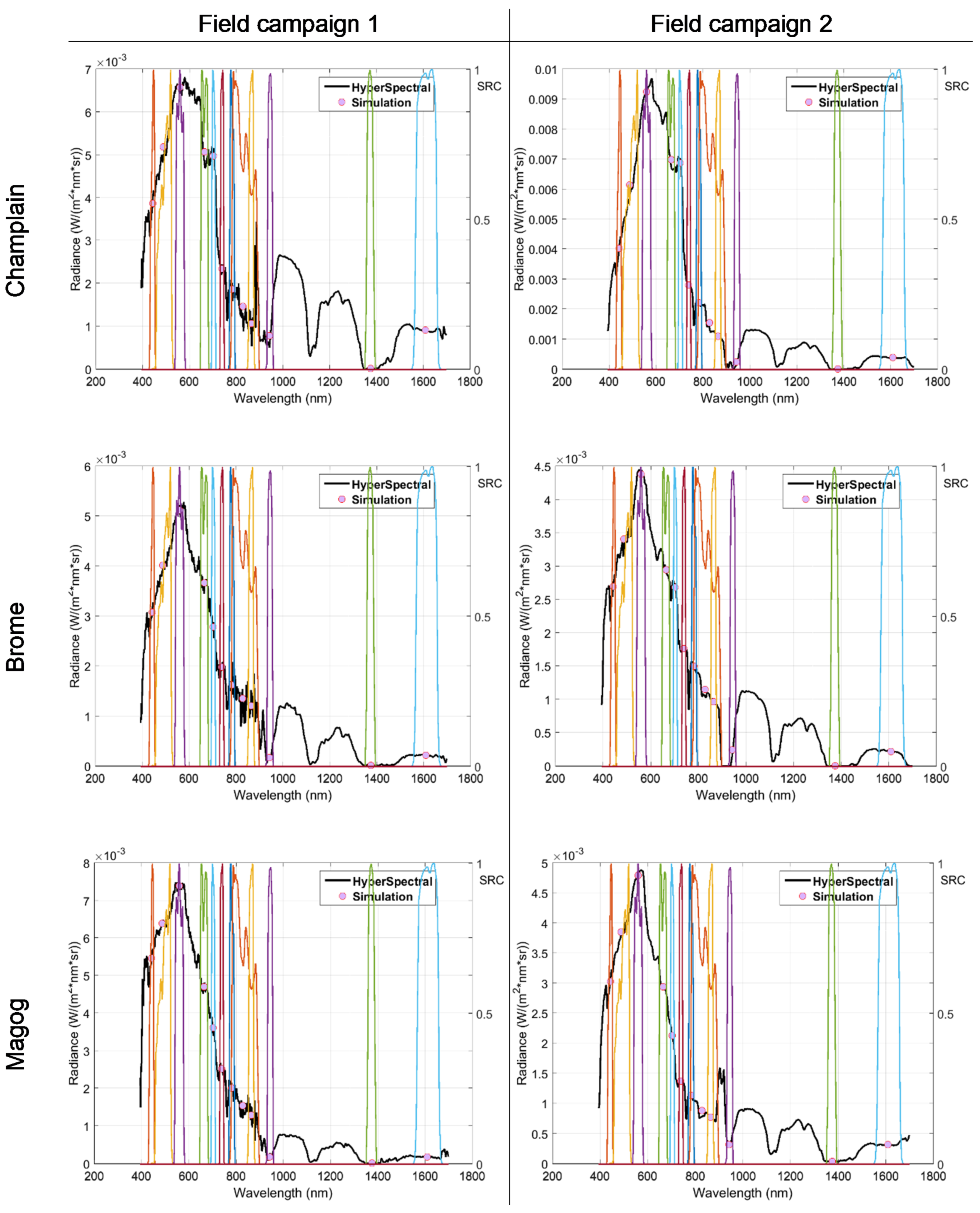
3.1.2. Hyperspectral Image Acquisition

The imaging engine used in this project is composed of a hexacopter drone loaded with hyperspectral cameras: Pika II (covering wavelengths from 400 to 900 nm) and Pika NIR (covering from 900 to 1700 nm). The spectral resolution of the Pika II is 3 nm, whilst it is 6 nm for the Pika NIR. Since the payload of the hexacopter drone is about 10 kg, it was necessary to make two overflights (a first with Pika II and a second with the Pika NIR) for each field campaign. The hexacopter drone was placed at 100 m altitude allowing image recording with a spatial resolution of 3 cm. However, since the goal is to develop a model applicable to Sentinel-2 data sensors, during the geo-rectification, the outputs were up-scaled to 20 m spatial resolution.
The Pika Hyperspectral sensor initially records the sunlight radiance in digital numbers (DN). Equation (1) was thus used to convert the DN to spectral radiance.
Spectral   radiance   = Gain   × DN   +   BIAS
Figure 5 shows results of the radiances collected over the nine sampling points of the three lakes in each FC. Each plot illustrates the average ± the standard deviation of the radiance recorded over in situ measurements. As can be seen, the largest variation is observed for FC 2 of Champlain Lake and the lowest is observed for FC 2 of Magog Lake. These observations highly concord with in situ chl_a measurements, where the maximum of the variation was also observed for FC 2 of Champlain Lake and the minimum of the variation was observed for FC 2 of Magog Lake (Figure 3).

3.1.3. Sentinel-2 Bands Simulation

The simulation of Sentinel-2 bands was performed based on its Spectral response curves (SRC) using Equation (2), inspired by the work of Blonski, et al. [34]. These SRC store information about the measured spectral responses and about the spectral width of each band. Since Sentinel-2A and -2B are twin sensors, their SRC are almost identical. Figure 6 shows the results of the simulation. The black lines represent the hyperspectral radiance recorded by the drone, the red dots represent the simulated radiance for each band using its corresponding SRC, and the colored lines are the plots of the Sentinel-2 SRC. It is important to highlight that the plotted hyperspectral radiances and their simulations are the averages picked up over the in situ measurements for each FC. From Figure 6, it is clear that Sentinel-2 bands are simulated without any loss of information, as all the simulations (red dots) are located on the initially signal recorded (black lines).
R A D _ s i m i = ( h y p _ R A D i × S R C i )
where:
R A D _ s i m i is the simulated radiance of band i;
h y p _ R A D i is the hyperspectral radiance of band i;
S R C i is the curve spectral response of band i, where   S R C i = 1 .

3.1.4. Simulated Bands Reflectance

In remote sensing applications, particularly in a multi-temporal context, it is better to use the reflectance instead of the radiance. In fact, the radiance is the spectral flux that reaches the satellite sensor determined both per unit of area and solid angle, whilst the reflectance is equal to the radiance divided by the irradiance and by other parameters for geometric considerations (Equation (3)). This eliminates the dependency on the instrument observing it or on the irradiance received. It is an intrinsic property of the surface, which only depends on illumination and observation angles. Thus, several advantages can be attributed to the use of the reflectance:
Its values are usually comprised between 0 and 1;
It is easy to compare the reflectance from one spectral band to another;
It is possible to compare the reflectance directly at different times of the year or of the day, since it is already corrected for variations of earth–sun distance and solar zenith angle (https://labo.obs-mip.fr/multitemp/les-grandeurs-radiometriques-eclairement-luminance-reflectance/, accessed on 4 February 2021).
Equation (3), known as the COST algorithm (Cosine of the sun zenith angle), inspired by the work of Moran, et al. [35], was used to estimate the reflectance of the simulated bands. It is an enhanced version of the DOS algorithm (Dark object subtraction). Indeed, in addition to the additive effect correction, such as the one used for the DOS algorithm, COST uses an additional correction for transmittance along the path from the ground toward the sensor (TAUz). The correction of this module, which is part of the multiplicative effect of the atmosphere, is made by the computation of the cosine of the solar zenith angle. According to Chavez Jr [36], the cosine of the solar zenith angle is a good approximation of TAUz.
R e f C O S T =   p i × ( L λ L h a z e ) × d 2 ( E S U N λ × C O S θ λ × C O S θ S )
where:
L λ is spectral radiance at the sensor’s aperture;
L h a z e is the upwelling atmospheric spectral radiance scattered in the direction of the sensor entrance pupil and within the sensor’s field of view [ W × m 2 × s r 1 × μ 1 ] ;
d is the earth–drone distance;
E S U N λ is the mean solar exo-atmospheric irradiance;
θ λ is the approximation of the atmospheric transmittance terms;
θ S is the solar zenith angle in degrees.
Figure 7 shows the results of the reflectance computed using the COST algorithm. The results presented here are averages of the reflectance picked up over the sampling points with their corresponding in situ chl_a measurements. It is important here to point out that the reflectance obtained are typical to case-2 water bodies, as the ratio of blue to green bands is clearly lower than 1.0 [37]. In addition, it reveals a relatively important signal backscattering, in the red-edge part of the spectrum, that is only perceived for high values of chl_a (Champlain Lake). This behavior is typical to water highly ladened with chl_a, which is the case of the Champlain Lake (>25 µg chl_a L−1).

3.2. Validation Database

3.2.1. In Situ Measurements

The Voluntary lakes monitoring network (VLMN) is a multiple partnership organization (environmental ministry, municipalities, university researchers, and water associations) that aims to: (1) acquire data to establish the trophic level of a large number of lakes and follow their evolution over time; (2) detect lakes showing signs of eutrophication and degradation; (3) educate, raise awareness, support, and inform local residents’ associations and other participants; and (4) draw a global portrait of the situation of resort lakes in Quebec. The VLMN has been operational since 2004, and since then, it has collected several water quality parameters (chl_a, water transparency, phosphorus, dissolved organic carbon, etc.), each year, over many inland freshwater bodies in Quebec. These data were used to validate the developed EBS using images acquired by the Sentinel-2A and -2B sensors.
A database of approximately 1891 samples was collected by the VLMN between the years 2015 and 2017. However, this number has been reduced to 94, spread over 89 inland waterbodies, due to three main reasons: 1) the number of cross-over dates (sampling and passage of satellite) was very low; 2) samples outside the Sentinel-2A and -2B tiles; and 3) the presence of haze or cloud. Table 2 summarizes the results of chl_a concentrations that have been used to test the performance of the EBS using a completely blind database. For 2015, it was not possible to cross-over any dates; thereby data collected from this year were not used in this validation process. The minimum measured value was 0.7 µg chl_a L−1 and the maximum was 41.8 µg chl_a L−1. Unlike the calibration database, most of the validation chl_a concentrations are centered at around 5 µg chl_a L−1 (Figure 8), meaning that most of the tested waterbodies belong to the oligotrophic level.

3.2.2. Remote Sensing Data

The remotely sensed data used in this project were obtained from Sentinel-2 Level 1 available on the Copernicus server. The Sentinel-2 sensor is boarded on two platforms (A and B) belonging to the European Space Agency. The Sentinel-2A was launched first (23 June 2015). Two years later, the Sentinel-2B followed it (7 March 2017). It records across a quite wide range of the spectrum covering 13 spectral bands (443–2190 nm), with a swath width of 290 km, and spatial resolutions of 10 m (for the visible bands), 20 m (red edge to shortwave of infrared (SWIR)), and 60 m (coastal blue and the atmospheric correction bands). For this study, only cross-over dates of Sentinel-2A and -2B passage to the VLMN in situ measurements were downloaded and pre-processed (Table 2). In order to increase the number of Sentinel-2 bands, the 10 m spatial resolution bands were upscaled to 20 m for a total of 9 bands covering parts from the blue (497 nm) to SWIR (1610 nm).

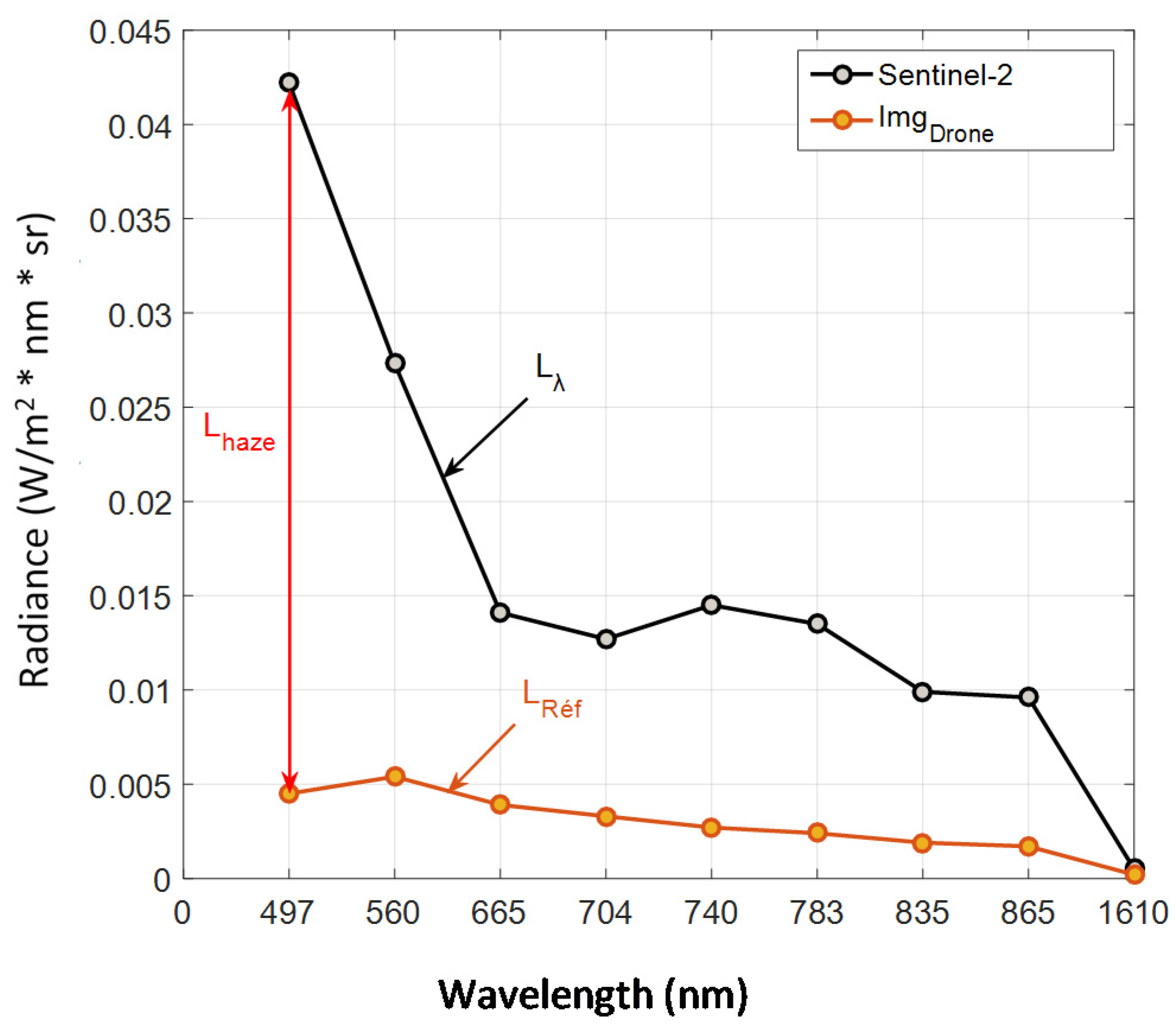
3.2.3. Atmospheric Correction of Sentinel-2 Images

Sentinel-2 Level 1 is radiometrically corrected and offers the Top of Atmosphere (ToA) reflectance. This product is, however, still affected by atmospheric effects and needs to be corrected. The Sentinel-2 bands were corrected, to the Bottom of Atmosphere (BoA) reflectance, using an adapted algorithm of the COST model. In fact, contrariwise to the simulated bands, where the L h a z e term of Equation (3) was insignificant (because images were recorded at 100 m altitude), this term is very significant for the Sentinel-2 bands and it has been necessary to correct it. The correction of this term is usually performed using the dark object subtraction technique [36]. However, when this technique was tested, it was perceived that the corrected reflectance of Sentinel-2 images was still influenced by the atmosphere (Figure 9A); the magnitude of the COST reflectance is significantly higher from those of the drone image ( I m g D r o n e ) (Figure 9A plot)).
Reflectance at the ToA and at the BoA using COST and C O S T M o d of a Sentinel-2 image (11 August 2017) are compared to reflectance of I m g D r o n e (14th August 2017) of Magog Lake and results are presented in Figure 9A. Results demonstrate that reflectance using the C O S T M o d approximates the best the reflectance of the I m g D r o n e and are confirmed by the plot in Figure 9B, where the R2 = 1.0 ( I m g D r o n e and C O S T M o d (a modified version of COST) reflectance are so close that they are superimposed in the Figure 9A plot). In fact, identifying the dark pixel using the standard COST model has some issues in an automated mode. In this study, a novel technique was developed using the radiance of the I m g D r o n e in order to fix this issue. Indeed, the most important term to be estimated in Equation (3) is the L h a z e . To reach a good estimation of the BoA reflectance, this term has to be the closest to the radiance of oligotrophic water bodies, since the absorption of the sunlight in these kinds of waterbodies is very high and, consequently, they are good samples of the dark pixels ground entities.
As per in situ measurements results (Table 1), Lake Magog can be classified as an oligotrophic water body. The radiance averages of each simulated band of this lake were used as a reference radiance to corrected Sentinel-2 images for the atmosphere effects, as presented in the Figure 10. L λ , in this figure, correspond to the radiance of the dark object (i.e., the minimal radiance corresponding to 1% reflectance) of the Sentinel-2 image that is used to compute the L h a z e . The L h a z e was simply the difference between the L λ and L R e f . Thus, the correction of the L h a z e was based, this time, on a reference that is known to be a “real” dark object.
Computing the L h a z e for each band of the Sentinel-2 image using the reference radiances yielded good results when applied manually (at a local-scale). On the other hand, at a regional-scale, the results significantly dropped. In fact, the main issue with this technique is that, from one band to another, the L λ of the dark pixel changes, and consequently, the intrinsic relationships between Sentinel-2 bands were destroyed. To fix this issue, once the Sentinel-2 dark pixel is identified for the blue band (since it is the most affected by the atmosphere), radiance coefficients are computed based on the radiance value of this pixel. These radiance coefficients are equal to the ratio of each band to the blue (Equation (4)). Thereby, the intrinsic behavior of the dark pixel is kept unchanged. Contrariwise to the first technique, solely the blue band radiance is used as a reference to correct for the L h a z e (s) of the rest of the Sentinel-2 bands. Thus, by adding these modifications to Equation (3), it took the form of Equation (5).
C o e f = L ( λ ) D P L ( b l u e ) D P
where:
L ( λ ) D P is the radiance of the dark pixel for a given band (λ);
L ( b l u e ) D P is the radiance of the dark pixel blue band.
R e f C O S T =   p i × ( L λ [ 0.0023 × C o e f λ ] ) × d 2 ( E S U N λ × C O S θ λ × C O S θ S )
where:
L λ is spectral radiance at the sensor’s aperture;
0.0023 is the averaged radiance recorded at the camera boarded on the drone;
C o e f λ is the correction coefficients as described in Equation (4);
d is the earth–sun distance in astronomical units;
E S U N λ is the mean solar exo-atmospheric irradiance;
θ λ is the approximation of the atmospheric transmittance terms;
θ S is the solar zenith angle in degrees.
The spectral reflectance presented in the red frame of Figure 11 illustrates the result of the C O S T M o d algorithm based only on the blue band radiance as a reference, while the spectral reflectance presented at the blue frame illustrates the result of the C O S T M o d algorithm based on all bands radiance as a reference. It is clear that the reflectance along the spectrum (from the blue to NIR) picked up from the image corrected with the C O S T M o d blue band radiance-based is closer to the known case-1 water spectral behavior. On the other hand, correcting independently the L h a z e for each Sentinel-2 band leads to destroying of the intrinsic physical relationships along the spectrum within the image. This fact is more tangible in the case of waters since the returned signal is initially too small and any slight over- or under-estimation of the L h a z e could change the initial spectral behavior, as shown in the blue frame of Figure 11.

4. Methodology and Statistical Evaluation Indices

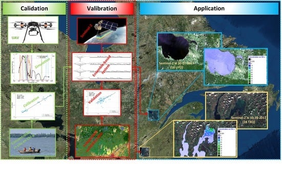
4.1. Methodological Approach

The flowchart presented in Figure 12 summarizes the methodological approach of this study. Two main steps were followed during this process: calibration, where two field campaigns were performed over three lakes. This step aims to collect in situ water samples and to record hyperspectral images using a drone, simultaneously. Water samples were analyzed in the laboratory for chl_a and other water properties, whilst drone images underwent several pre-processing phases:
Geometric and radiometric (Equation (1)) corrections;
Upscaling to 20 m spatial resolution (equal to that of Sentinel-2);
Sentinel-2 spectral bands simulation (Equation (2));
Simulated bands reflectance computation (Equation (3)).
Once these steps were finalized, it was a question to calibrate an ensemble-based system (EBS) to estimate chl_a concentration and to evaluate its performance locally using the Leave-one-out cross-validation (LOOCV) technique (EBS development will be more detailed in the next section). Once the EBS reached an acceptable rate of errors, this closes the first step of the methodological approach. The second part focused on validating and testing the robustness of the EBS at a regional scale. Thus, the EBS was challenged over several inland waterbodies belonging to different geo-environmental regions (Figure 1). Hence, it was a question of collecting chl_a in situ measurements from several environmental organizations, particularly the VLMN, qualified here as a blind database. Cross-over dates of Sentinel-2 images to in situ samples were downloaded and pre-processed to the BoA reflectance (Equation (5)). Sentinel-2-based chl_a concentration products were, as a final step, compared to in situ chl_a collected by the VLMN.

4.2. Ensemble-Based System

Seeking additional opinions before making a decision is part of human nature. The general concept behind EBS algorithms is based on this principle. In fact, an EBS is composed of several individual elements (classifiers and/or estimators). Combining the decision of these individual elements decreases modeling errors in contrast to an estimation based on a unique model that can be erroneous and consequently, increases the error [23]. Two main keys are required for building a robust EBS: 1) reaching the highest possible diversity between its individual elements and 2) finding the best combination rule of individual elements so that correct decisions are amplified and the incorrect ones are canceled out [23]. This technique is principally used in sensitive fields such as medical care [38,39,40], financial businesses [41,42,43], and recently was used to remote estimate chl_a using MODIS data [15].
On the other hand, the WHO has established the value of 10 µg chl_a L−1 as the first alert level to freshwater bodies use for recreational activities [44]. In this context, many studies have demonstrated that the returned signature from oligotrophic waterbodies is different compared to that returned from mesotrophic or eutrophic waterbodies [45,46,47], meaning that sensitive spectral regions to water bodies highly laden in chl_a are not necessarily the same for water bodies moderately or poorly laden in chl_a concentrations. As a consequence, using a specific model to each trophic level could enhance the quality of chl_a estimates than using a unique model for all trophic levels [48]. Taking into account the above statements, it was decided to develop a hybrid EBS composed of an Ensemble-based classifier (EBC) and an Ensemble-based estimator (EBE).

4.3. Statistical Indices for the Ensemble-Based System Assessment

Performance evaluation of the model in both cases (using the LOOCV technique or using the blind dataset) was performed using five statistical indices (Coefficient of determination (R2), bias, Root mean squared errors (RMSE), the Nash criterion (Nash), and the relative errors). The Nash criterion evaluates the performance by comparing the estimated values to the in situ measurements average, producing a result that ranges between −∞ and 1.0 (inclusive). A negative Nash means that it would be better to use the in situ measurements’ average than the model estimates, whereas values between 0.0 and 1.0 are generally viewed as acceptable levels of performance, and model performance is satisfactory for values higher than 0.8; the model is perfect when Nash = 1.0. The mathematical Equations (6)–(10) of the indices are as follows:
R 2 = [ i = 1 n ( M i M ¯ ) ( E s E s ¯ ) i = 1 n ( M i M ¯ ) 2 i = 1 n ( E s i E s ¯ ) 2 ] 2
B I A S r = 1 n i = 1 n ( E s i M i )
R M S E =   1 n i = 1 n ( E s i M i ) 2
N A S H = 1 i = 1 n ( M i E s i ) 2 i = 1 n ( M i M ¯ ) 2
R e l a t i v e   e r r o r = ( M i E s i ) M i   × 100
where:
n is the database size, M and Es are measured and estimated values, and M ¯ and E s ¯ are averages of measured and estimated values.

5. Results and Discussion

5.1. The Ensemble-Based Classifier Development

Two levels in chl_a loads (> 10 µg chl_a L−1 representing mesotrophic and eutrophic waterbodies and < 10 µg chl_a L−1 representing oligotrophic waterbodies) were used in this study. For discrimination purposes, the Classification and regression tree (CART) algorithm was applied [49]. The CART algorithm has selected R λ 4 R λ 5 as the best discrimination index. However, such kinds of algorithms are known to be local and unstable [50]. In fact, the proposed decisions tree by the CART is optimal for the used training database, but not unique. A simple modification within this database can lead to radical changes in the decisions tree. An interesting way to control this uncertainty is to quantify it and to take it into consideration when estimating chl_a concentrations. The control of the CART uncertainty was possible by using the bagging algorithm (n-resampling with replacement; nbag was set to 25,000 iterations in this study) based on the preselected discrimination index. This allowed a random vector (v) to be generated composed by thousands of thresholds.
Normally, all these thresholds generated should be implied in the classification process, but this will surely demand a huge running time as images are composed of hundreds of thousands of pixels. Thus, the Gaussian quadrature method [51] was used for optimizing the runtime. The purpose of this method is to summarize a given distribution in some optimal points (referred to here as optimal thresholds) of this distribution that approximates it the best. Thereby, based on the random vector, it was possible to establish a probability distribution characterized by a mean (µ) and a variance (σ). These two statistical moments have served after that to develop the EBC (beige frame in Figure 13) composed of three (arbitrary choice) Optimal thresholds ( Opt Thr ) that are the Lower, Upper, and Nominal thresholds, based on the Gaussian quadrature method, using the following equations:
N o m i n a l T h r = μ ( v )
L o w e r T h r = μ ( v ) 3 × σ ( v )
U p p e r T h r = μ ( v ) + 3 × σ ( v )
where μ ( v ) and σ ( v ) are the mean and variance of the random vector, respectively.

5.2. The Ensemble-Based Estimator Development

Based on the EBC results, it was possible to develop an EBE. Indeed, by means of the Nominal threshold ( N o m i n a l T h r ), Lower threshold ( L o w e r T h r ), and Upper threshold ( U p p e r T h r ), it is possible to subdivide the calibration database into six ( 3 Opt Thr × 2 Classes ) sub-classes and four modeling spaces (Figure 13). Each sub-class is composed of a dataset of chl_a measurements that are used to train a specific estimator (known as expert in the machine learning field). The subdivision was made as follows. Three datasets specific to oligotrophic waterbodies are composed of chl_a samples where the values of R λ 4 R λ 5 (the discrimination index) are, respectively, inferior to the N o m i n a l T h r , L o w e r T h r , and U p p e r T h r (blue arrows in Figure 13), referred as { Exp OT i } in this study. Additionally, three datasets specific to mesotrophic and eutrophic waterbodies are composed of chl_a samples where the values of R λ 4 R λ 5 are, respectively, superior to the N o m i n a l T h r , L o w e r T h r , and U p p e r T h r (red arrows in Figure 13), referred to as { Exp OT i } . These sets of experts are the individual elements of the EBE (blue frame in Figure 13). It is, however, important to point out that it was not possible to train six different experts in this study. As shown in Figure 13, there are no chl_a samples located in the transition zone (area between dashed green ( L o w e r T h r ) and blue ( U p p e r T h r ) lines). As a consequence, it was possible to train only a unique expert for each class instead of three each (calibration plots in Figure 13).

5.3. The Hybrid Ensemble-Based System for Chlorophyll-a Modeling

Estimation of the chl_a using this hybrid EBS is made on two steps: (1) determination of the Modeling space (MS) by means of the EBC and (2) the estimation of the chl_a concentration using the corresponding expert to the pre-identified MS. For the proposed approach, 4 MSs are identified as illustrated in the blue frame of Figure 13. The estimation of chl_a using this approach is weighted average-based. Weighting coefficients ( ω ) , 1/6 for the L o w e r T h r and U p p e r T h r and 2/3 for the N o m i n a l T h r , are computed from the Gaussian quadrature method, as demonstrated by Tørvi and Hertzberg [51]. Experts’ weights of chl_a estimates change depending on the MS. However, the sum of the used weights in each case is always equal to 1.0. Thus, chl_a estimation using the ESB is performed as it is described in Figure 14. Even if it was not possible to train three different experts per sub-class, as is supposed to be the case, we have deliberately detailed the calculation process, as if this were the case, for those interested for their future work.

5.4. Calibration of the Experts

Once the calibration database was subdivided, it was a question training the different experts. To do this, all possible combinations of two- and three-band normalized indices were computed, for each dataset, and integrated in a stepwise regression. For mesotrophic and eutrophic waterbodies, three spectral indices were selected by the stepwise as the best estimator to retrieve chl_a and were able to explain 93% (Figure 13) of its variance (Equation (14)). For oligotrophic waterbodies, solely a unique spectral index was selected by the stepwise as the best estimator to retrieve chl_a and was able to explain 47% (Figure 13) of its variance (Equation (15)). As stated above, it was only possible to calibrate two experts in this work. This is due to a lack of moderate chl_a values in the initial database, notably between 5 and 15 µg chl_a L−1 (Figure 3). Since the discrimination threshold used here was 10 µg chl_a L−1 (as proposed by the WHO), there was a significant gap in the classification results within the transition area between the two classes (dashed lines in Figure 13) and consequently, only two datasets were set instead of six.
Based on the stepwise regression results, the expert designed to estimate chl_a of mesotrophic and eutrophic waterbodies is trained by six different spectral regions ranging from the blue to NIR. This spectral richness led to the development of a strong function of calibration in these blooming conditions. The green, red, and NIR parts of the spectrum have already been used, by many researchers, to estimate the chl_a in mesotrophic and eutrophic water bodies [52,53]. The contribution of the blue band in retrieving chl_a in these blooming conditions was not expected. However, it is important to take into consideration that the blue band was used in a three-band normalized index including the red and NIR bands. This combination of bands has, somehow, highlighted a significant relationship between this spectral index and the chl_a. On the other hand, the expert designed to estimate chl_a of oligotrophic waterbodies is trained by a simple function using a two-band normalized index. The used bands are located in the green and red parts of the spectrum. This result is coherent with other work results that have related the estimation of chl_a to its bio-optical activity that is more correlated to the visible parts of the spectrum [54].
[ C h l a ] M e s o e u t r o p h i c = exp ( 2.72   I n d 1 + 3.39 I n d 2 + 3.23 I n d 3 + 2.21 )
with
  • I n d 1 = B a n d 3 B a n d 7 B a n d 3 + B a n d 7
  • I n d 2 = B a n d 3 B a n d 8 B a n d 3 + B a n d 8
  • I n d 3 = ( B a n d 5 B a n d 2 B a n d 5 + B a n d 2 + B a n d 5 B a n d 4 B a n d 5 + B a n d 4 ) B a n d 2 B a n d 4 B a n d 2 + B a n d 4
[ C h l a ] O l i g o t r o p h i c = exp ( 3.35 I n d 4 + 1.93 )
with
  • I n d 4 = B a n d 3 B a n d 5 B a n d 3 + B a n d 5
where: band2 = 497, band3 = 560, band4 = 665, band5 = 704, band7 = 783, and band8 = 835 nm.

5.5. Cross-Validation: Local Evaluation

In order to evaluate the local performance of the developed approach, the cross-validation technique was used. This technique consists of removing a sample (or a set of samples (known as k-fold cross-validation)) from the calibration database, to use the remaining samples to train a new model, and to estimate the chl_a concentration of the removed sample with the trained new model (known as LOOCV). This exercise is re-done for the whole calibration database. It is, however, important to underline that this technique was adapted for the EBS. In fact, each removed sample was first classified by means of EBC. Thereafter, the estimation of the chl_a concentration was done using the corresponding EBE-expert to the classification result. With this technique, it was possible to compare observed to estimated chl_a concentrations using the pre-mentioned statistical indices (Equations (6)–(10)).
Figure 15 shows the LOOCV result of chl_a estimates. It is important to point out that the above processing and results are based only on the simulated Sentinel-2 reflectance recorded by the drone. The R2 and Nash of 0.94% underscore the robustness of the EBS. The accuracy and exactitude of the EBS can be considered as high (RMSE = 5.6 µg chl_a L−1) to very high (bias almost null). These high performances are also supported by the distribution of the dots around Line 1:1 that emphasize the absence of any under- or over-estimation, particularly at the extremities (Figure 15A). The above findings are confirmed by the residuals plot (Figure 15B) result, where the relative errors range between −0.8% and 0.6% and are distributed around 0%, highlighting the absence of any form of trends. Additionally, it is perceived that the relative error is reduced by almost 60% for values higher than 40 µg chl_a L−1. This was somewhat expected since the expert designed to estimate chl_a concentration in these blooming conditions was able to explain up to 93% the chl_a variance (Figure 13).

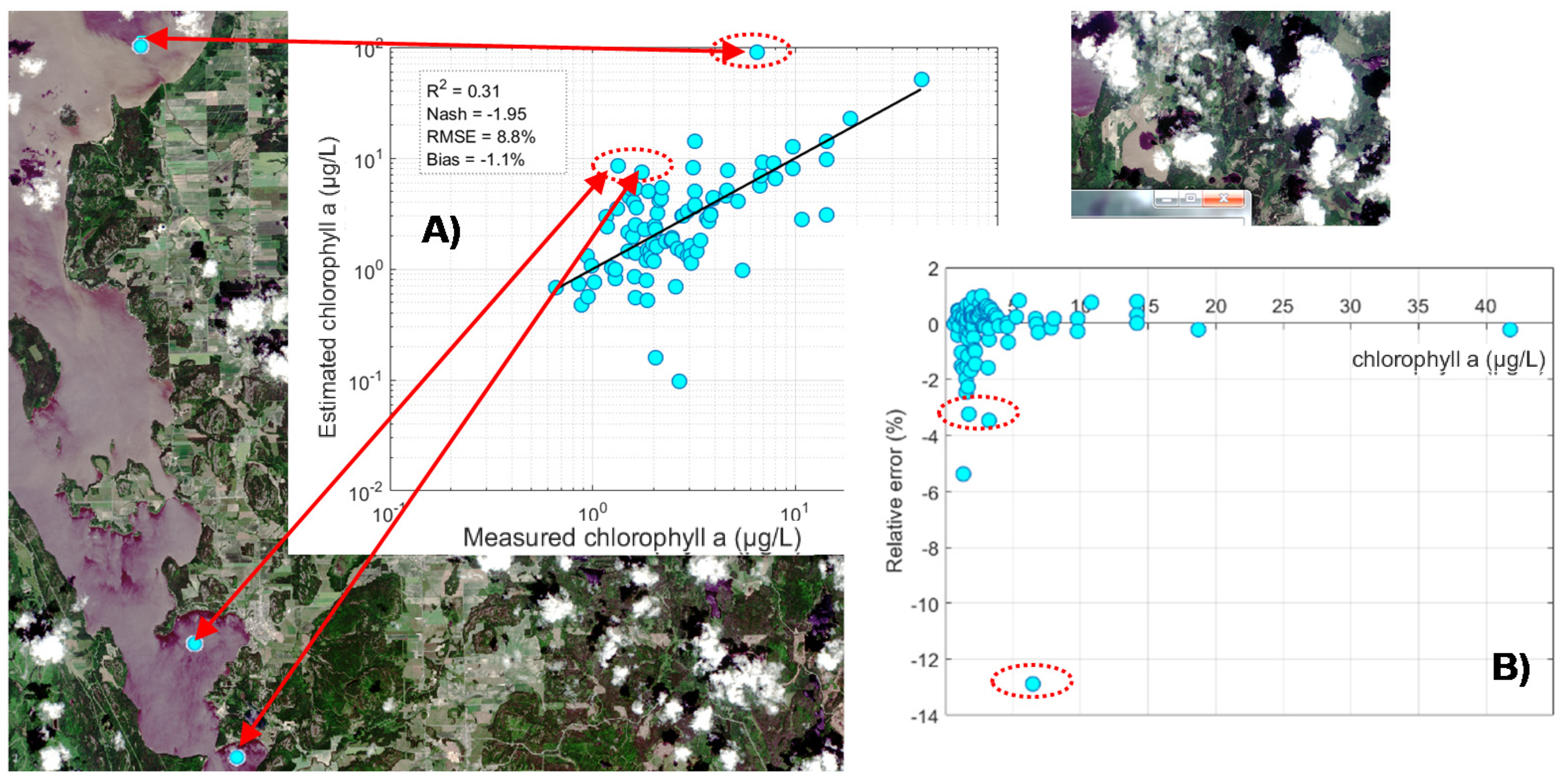
5.6. Validation with the Blind Dataset: Regional Evaluation

Figure 16 shows the results of EBS evaluation using the blind databases. The performance of the EBS can be considered as low (R2 = 0.31) to very low (Nash = −1.95). However, considering the results of the bias (−1.1 µg chl_a L−1) and the RMSE (8.8 µg chl_a L−1), it can be concluded that in most cases, the estimation of chl_a is accurate and exact (Figure 16A). These conclusions also emerge in the residuals plot where almost all the residues are plotted around 0%, except for some specific cases (Figure 16B). Even if the Nash is negative, meaning that the average of the measured chl_a concentrations is more accurate than the chl_a modeling using the EBS, the low rate of the RMSE and residuals distribution around 0% with relative errors comprised between −2% and 2%, in most cases, encouraged us to investigate further in our research. In fact, based on the Figure 16B, only four estimates are tainted with a high error (relative error < −3%). When these last estimates were traced in the blind database, they all belonged to inland waterbodies affected by very high turbidity (dashed arrows and circles in Figure 16). (The fourth sample was on another Lake, to lighten the paper, this last case was not illustrated.)
When these four samples were removed from the blind database, the results increased significantly (Figure 17). A R2 of 0.85 and a Nash of 0.79 underline the good performance and the robustness of the EBS to retrieve the chl_a using data recorded from Sentinel-2A and -2B sensors. The RMSE dropped to 2.4 µg chl_a L−1 and the bias is null (Figure 17A). These two last statistical results highlight the high exactitude and accuracy of the EBS estimates. It is interesting to point out that chl_a concentrations of the blind database are very low (97% are inferior to 10 µg chl_a L−1 and 95% are inferior to 5 µg chl_a L−1 (Figure 8)). Chl_a modeling errors are known to be high in such conditions, as the signal-to-noise ratio is often high, because of the low signal magnitude returned by the chl_a that is almost equal to water backscattering and to the retuned signal from other bio-optical components in the water column (total suspended solids, colored dissolved organic matters, etc.). Despite these facts, chl_a modeling error rates using the EBS on Sentinel-2 data remained low with relative errors comprised between −1% and 1% for values higher than 5 µg chl_a L−1 and relative errors between −2.5% and 1% for values lower than 5 µg chl_a L−1 (Figure 17B).

5.7. Spatial Distribution Assessment of the Ensemble-Based System

Figure 18 shows three examples of practical applicability of the EBS on Sentinel-2 images. The blue frame illustrates a zoomed section of Lake Saint-Jean with clear water partially covered by a thin haze. The outputs of chl_a concentrations over this lake are below 5 µg chl_a L−1 even in the hazy section. This clearly demonstrates that the chl_a estimated by the EBS are not affected by the thin haze. The yellow frame illustrates a zoomed section of Lake Saint-Pierre. This water body is known by its high loads of suspended solids. In fact, according to the environmental Ministry of Quebec, the annual average suspended solids (https://www.environnement.gouv.qc.ca/eau/Atlas_interactif/evolution/pdf/05300004_TTEND_MES.pdf, accessed on 4 February 2021) load in Lake Saint-Pierre for the year 2017 was approximately 163 mg/L, whilst the annual average chl_a (https://www.environnement.gouv.qc.ca/eau/Atlas_interactif/evolution/pdf/05300004_TTEND_CHLO.pdf, accessed on 4 February 2021) was about 5.85 µg/L1. Estimates derived from the EBS of chl_a for Lake Saint-Pierre are between 0.1 and 5 µg/L1, as shown in Figure 18. This is a good demonstration that the EBS is not affected by high loads of suspended solids in inland waterbodies. Finally, Missisquoi Bay of Lake Champlain experienced a huge harmful algae bloom on October 10, 2017 captured by the Sentinel-2 sensor. Estimates from the derived EBS of chl_a copy the spatial distribution of this bloom well, while in areas where the bloom did not occur, chl_a estimates have remained very low. The three examples above highlight the applicability of the EBS, with a high level of reliability, for monitoring harmful algal blooms using Sentinel-2 data.

6. Challenges, Advantages, and Limitations of Chlorophyll-a Monitoring Using UAVs and Satellites Data

The quality of surface water is affected by climate and human activity and affects climate, biological diversity, and human well-being. For the last few decades, efforts by many scientists have been made to monitor water quality, notably chl_a concentration, using remote sensing data. In most cases, the developed models yielded success within the calibration sites, but their estimates were mostly inaccurate outside these sites. The big challenge of this study was thus to achieve acceptable accuracy rates at a local (within the calibration sites) and a regional (outside the calibration sites) scale. This goal was partially accomplished by using one of the most promising techniques in machine learning—the EBS. On the one side, modeling quality, locally and regionally, indeed yielded satisfying rates of accuracy (higher than 85%). On the other side, at both scales, it has been perceived that errors increase with low chl_a concentrations. This fact was more tangible in the case of validation with the blind database. Many researchers link this high rate of error to the atmosphere effect and our results support this assumption as the relative errors were lower using data collected by the drone (100 m altitude) than those collected by Sentinel-2 data (786 km altitude). In addition, the atmospheric model used (COST) in this study is based on the assumption of at-water leaving reflectance of dark object being equal to 1%. A new selection method of the dark object, based on the hyperspectral image, was proposed and yielded higher accuracy than the standard one. However, the small image stripe does not cover a large part of the Sentinel-2 images. This fact could be a limiting factor, decreasing the accuracy of the atmospheric correction in regions further away than those covered by the hyperspectral image. More investigations must be conducted, in this field, to achieve more accurate estimates of the BoA at-water reflectance.
The developed hybrid EBS has demonstrated its ability to model chl_a using the drone-simulated Sentinel-2 data and using data recorded by the two Sentinel-2 sensors. This is a double added-value to the EBS use. In fact, it is possible, using the same algorithm, to use two sources of data to monitor algae bloom. Indeed, Sentinel-2 sensor data-based chl_a products could be used, as stated above, on a regional-scale for spatial monitoring of algae blooms as well as for their temporal recurrence. Water managers and stakeholders are constantly looking for such monitoring tools for their decisions-making. On the other hand, UAVs are nowadays affordable and easy-to-use (almost fully autopiloted) more than ever. Furthermore, cameras such as the Tetracam MicroMCA-global shutter model have the ability to be set by personalized wavelength filters that can cover the same exact spectral regions as used to estimate the chl_a using the EBS. Thereby, it is possible to develop a low-cost engine for chl_a retrieval for local and personalized use anytime and anywhere. This offers great flexibility of use (time, space, and sensor characteristics), which could also be of great help to managers and stakeholders in specific crises. Through the approach developed, it is now possible to harness the strength of these two complementary technologies for the benefit of better-quality management of freshwater bodies.
The transposable application capacity (from UAVs towards satellites data and vice versa) could open up new ways of exploiting previous databases (known as Spatial database (SB) in remote sensing) to train models for the future generation of sensors and use their very first data delivered with an acceptable modeling rate without any delay necessary to collect a new SB specific to this sensor. Indeed, thanks to the SB already pre-collected, it would be possible to simulate the bands of the new sensor and to train a new model, based on machine or deep learning algorithms, that will be compatible with the images acquired by this new sensor. Additionally, the performance of already trained and operational models could be enhanced by means of the proposed approach. In fact, since most operational models are data-oriented, retraining them with their original SB merged with an SB built from simulated bands (specific to their bandwidth and spectral regions) will certainly help improve their modeling performance.
However, it is also important to underline the limitations of these technologies. Cloud and haze are the big limiting-factors to use data from satellite sensors such as Sentinel-2. The temporal frequency could also, at some level, be a limiting factor to monitor algae blooms using Sentinel-2 data. In contrast, UAVs flights are more flexible in terms of temporal and space use, but the spatial coverage is very restrained compared to satellite data. Climate conditions, especially wind, are a big limitation for UAV use. In fact, depending on the model, there is always a wind use-threshold. Above that, it is not recommended to take-off. On the other side, in the case of a cloudy sky, the radiance recorded by the camera boarded on the UAVs is significantly affected by cloud shadow. It is often recommended to record image scenes in a uniform climate condition. With respect to EBS development, the accuracy of the modeling could be higher if more data were available, especially for concentrations between 10 and 20 µg chl_a L−1. This middle class was underrepresented in the calibration database and led to the training of only one expert, instead of three, in each trophic class. Averaging estimates of three experts would undoubtedly lead to greater accuracy in the modeling of chl_a. Finally, it should be noted that the EBS has shown a failure to estimate chl_a in waters affected by high turbidity. However, it can still be applied in an operational mode, since these waters are known to highly reflect in the red than in the green part of the spectrum. By using this information, it is possible to mask waters highly affected by turbidity before proceeding to chl_a modeling.

7. Conclusions

A hybrid EBS for chl_a estimates using Sentinel-2 simulated bands was developed and tested on freshwater bodies in southern Quebec using data recorded by Sentienl-2A and 2B sensors. Several innovative aspects were developed in this paper: (1) development of a hybrid EBS composed of EBC and EBE; (2) calibration of EBS using Sentinel-2 simulated bands; (3) testing the EBS using data recorded by Sentinel-2A and 2B; and (4) the use of the Gaussian quadrature function for time running optimization. Combining these aspects has led to the development of a robust hybrid EBS to monitor chl_a concentrations in freshwater bodies at local and regional scales.
Two validation techniques were used to assess the performance of the proposed method: (1) the leave-one-out cross-validation, as a local evaluation of the EBS, and (2) validation with blind datasets (in situ and remotely), as a regional evaluation. The leave-one-out cross-validation results were satisfactory (R2 = Nash = 0.94). The hybrid EBS showed a relatively negative bias (−0.2 µg chl_a L−1) and the errors were relatively low (RMSE = 5.6 µg chl_a L−1). Validation with the blind datasets highlighted some failures of the EBS in estimating the chl_a in waters affected by high turbidity. Modeling the chl_a in these ecosystems is highly tainted by errors (Nash < 0). However, when the EBS was tested on waters not affected by high turbidity, the results significantly increased (R2 = 0.85, Nash = 0.79, RMSE = 2.4 µg chl_a L−1). Additionally, it has been perceived that the relative errors were comprised between −2.5% and 1% and have decreased by almost 60% when estimating chl_a values higher than 40 µg chl_a L−1. This is probably due to the reduced number of calibration data, notably medium values of chl_a, which were under-represented and to the higher signal-to-noise ratio for at-water leaving reflectance in oligotrophic waters.
The proposed method allowed the development of a robust approach to estimate chl_a in freshwaters using either Sentinel-2 data simulated from a hyperspectral camera boarded on a drone or data recorded by the Sentinel-2A and 2B sensors. Assessment of the spatial distribution pointed out that the modelling of chl_a using EBS is not affected by thin haze or suspended solids and is very sensitive to algal blooms. Overall, the performance of the hybrid EBS was satisfactory, except for water affected by high turbidity. Despite this, EBS could still be used in an operational mode, in a complementary way using both technologies, since turbid water can be easily identified and masked before the chl_a modeling. Such a tool could be of great assistance to water managers and stakeholders for better water quality assessment, particularly in areas with abundant lakes like the province of Quebec and Canada.

Author Contributions

Conceptualization, A.E.-A. and K.C.; methodology, A.E.-A. and K.C.; validation, A.E.-A., A.V., and L.R.; formal analysis, A.E.-A.; resources, J.-P.D.; data curation, H.A.; writing—original draft preparation, A.E.-A.; writing—review and editing, A.E.-A., K.C., A.V., L.R., and J.-P.D.; visualization, A.E.-A.; supervision, K.C.; project administration, A.E.-A.; funding acquisition, K.C. All authors have read and agreed to the published version of the manuscript.

Funding

This project was funded by the CSA (PDAOT no. 9F013 160225/003/MTB).

Institutional Review Board Statement

Not applicable.

Informed Consent Statement

Not applicable.

Data Availability Statement

All data collected, pre-processed, processed, or analyzed during this study are included in this work.

Acknowledgments

We are grateful to C. Prévost from Ressources Naturelles Canada and L. Champagne from the CSA for the follow of the progress all over the project. Special thanks to J. Poulin, the drone pilot. Our gratitude as well goes to I. Laurion from the “Institut National de la Recherche Scientifique” and C. Corbel, M. Trindade, and J. Camy from Group Hemisphere for collaborating in the project and help obtaining the in situ calibration dataset from the Voluntary lakes monitoring network of Quebec. Our thanks also go to the European Space Agency for Sentinel-2 data availability.

Conflicts of Interest

The authors declare no conflict of interest.

References

  1. Drobac, D.; Tokodi, N.; Simeunović, J.; Baltic, V.; Stanić, D.; Svircev, Z. Human exposure to cyanotoxins and their effects on health. Arch. Ind. Hyg. Toxicol. 2013, 64, 305–316. [Google Scholar] [CrossRef] [Green Version]
  2. Black, J.G.; Black, L.J. Microbiology: Principles and Explorations, 8th ed.; John Wiley & Sons: Hoboken, NJ, USA, 2012. [Google Scholar]
  3. Stoermer, E.F. Phytoplankton assemblages as indicators of water quality in the laurentian great lakes. Trans. Am. Microsc. Soc. 1978, 97, 2–16. [Google Scholar] [CrossRef]
  4. Long, S.; Hamilton, P.B.; Yang, Y.; Ma, J.; Chobet, O.C.; Chen, C.; Dang, A.; Liu, Z.; Dong, X.; Chen, J. Multi-year succession of cyanobacteria blooms in a highland reservoir with changing nutrient status, Guizhou Province, China. J. Limnol. 2018, 77, 232–246. [Google Scholar] [CrossRef] [Green Version]
  5. Rantajärvi, E.; Olsonen, R.; Hällfors, S.; Leppänen, J.-M.; Raateoja, M. Effect of sampling frequency on detection of natural variability in phytoplankton: Unattended high-frequency measurements on board ferries in the Baltic Sea. ICES J. Mar. Sci. 1998, 55, 697–704. [Google Scholar] [CrossRef] [Green Version]
  6. Blondeau-Patissier, D.; Gower, J.F.; Dekker, A.G.; Phinn, S.R.; Brando, V.E. A review of ocean color remote sensing methods and statistical techniques for the detection, mapping and analysis of phytoplankton blooms in coastal and open oceans. Prog. Oceanogr. 2014, 123, 123–144. [Google Scholar] [CrossRef] [Green Version]
  7. Gordon, H.R.; Clark, D.K.; Brown, J.W.; Brown, O.B.; Evans, R.H.; Broenkow, W.W. Phytoplankton pigment concentrations in the Middle Atlantic Bight: Comparison of ship determinations and CZCS estimates. Appl. Opt. 1983, 22, 20–36. [Google Scholar] [CrossRef]
  8. Bohn, V.Y.; Carmona, F.; Rivas, R.; Lagomarsino, L.; Diovisalvi, N.; Zagarese, H.E. Development of an empirical model for chlorophyll-a and Secchi Disk Depth estimation for a Pampean shallow lake (Argentina). Egypt. J. Remote Sens. Space Sci. 2018, 21, 183–191. [Google Scholar] [CrossRef]
  9. Di Cicco, A.; Sammartino, M.; Marullo, S.; Santoleri, R. Regional empirical algorithms for an improved identification of phytoplankton functional types and size classes in the Mediterranean sea using satellite data. Front. Mar. Sci. 2017, 4, 126. [Google Scholar] [CrossRef] [Green Version]
  10. Gholizadeh, H.; Robeson, S.M. Revisiting empirical ocean-colour algorithms for remote estimation of chlorophyll-a content on a global scale. Int. J. Remote Sens. 2016, 37, 2682–2705. [Google Scholar] [CrossRef]
  11. Watanabe, F.S.Y.; Alcântara, E.; Rodrigues, T.W.P.; Imai, N.N.; Barbosa, C.C.F.; Rotta, L. Estimation of chlorophyll-a concentration and the trophic state of the Barra Bonita hydroelectric reservoir using OLI/Landsat-8 images. Int. J. Environ. Res. Public Health 2015, 12, 10391–10417. [Google Scholar] [CrossRef]
  12. Duan, H.; Ma, R.; Xu, J.; Zhang, Y.; Zhang, B. Comparison of different semi-empirical algorithms to estimate chlorophyll-a concentration in inland lake water. Environ. Monit. Assess. 2010, 170, 231–244. [Google Scholar] [CrossRef]
  13. El-Alem, A.; Chokmani, K.; Laurion, I.; El-Adlouni, S.E. Comparative Analysis of four models to estimate chlorophyll-a concentration in case-2 Waters Using moderate resolution imaging spectroradiometer (MODIS) imagery. Remote Sens. 2012, 4, 2373–2400. [Google Scholar] [CrossRef] [Green Version]
  14. Moses, W.J.; Gitelson, A.A.; Berdnikov, S.; Povazhnyy, V. Estimation of chlorophyll- a concentration in case II waters using MODIS and MERIS data—Successes and challenges. Environ. Res. Lett. 2009, 4, 045005. [Google Scholar] [CrossRef] [Green Version]
  15. El-Alem, A.; Chokmani, K.; Laurion, I.; El-Adlouni, S.E.; Raymond, S.; Ratte-Fortin, C. Ensemble-based systems to monitor algal bloom with remote sensing. IEEE Trans. Geosci. Remote Sens. 2019, 57, 7955–7971. [Google Scholar] [CrossRef]
  16. Ferreira, M.S.; Galo, M.D.L.B. Chlorophyll a spatial inference using artificial neural network from multispectral images and in situ measurements. An. Acad. Bras. Ciências 2013, 85, 519–532. [Google Scholar] [CrossRef] [Green Version]
  17. Kown, Y.S.; Baek, S.H.; Lim, Y.K.; Pyo, J.; Ligaray, M.; Park, Y.; Cho, K.H.; Kwon, Y.S. Monitoring coastal chlorophyll-a concentrations in coastal areas using machine learning models. Water 2018, 10, 1020. [Google Scholar] [CrossRef] [Green Version]
  18. Aguirre-Gómez, R.; Salmerón-García, O.; Gómez-Rodríguez, G.; Peralta-Higuera, A. Use of unmanned aerial vehicles and remote sensors in urban lakes studies in Mexico. Int. J. Remote Sens. 2016, 38, 2771–2779. [Google Scholar] [CrossRef]
  19. Becker, R.H.; Sayers, M.; Dehm, D.; Shuchman, R.; Quintero, K.; Bosse, K.; Sawtell, R. Unmanned aerial system based spec-troradiometer for monitoring harmful algal blooms: A new paradigm in water quality monitoring. J. Great Lakes Res. 2019, 45, 444–453. [Google Scholar] [CrossRef]
  20. Flynn, K.F.; Chapra, S.C. Remote Sensing of submerged aquatic vegetation in a shallow non-turbid river using an unmanned aerial vehicle. Remote Sens. 2014, 6, 12815–12836. [Google Scholar] [CrossRef] [Green Version]
  21. Lyu, P.; Malang, Y.; Liu, H.H.; Lai, J.; Liu, J.; Jiang, B.; Qu, M.; Anderson, S.; Lefebvre, D.D.; Wang, Y. Autonomous cyano-bacterial harmful algal blooms monitoring using multirotor UAS. Int. J. Remote Sens. 2017, 38, 2818–2843. [Google Scholar] [CrossRef]
  22. Kislik, C.; Dronova, I.; Kelly, M. UAVs in support of algal bloom research: A review of current applications and future op-portunities. Drones 2018, 2, 35. [Google Scholar] [CrossRef] [Green Version]
  23. Polikar, R. Ensemble based systems in decision making. Circuits and Systems Magazine, IEEE 2006, 6, 21–45. [Google Scholar] [CrossRef]
  24. Du, P.; Xia, J.; Zhang, W.; Tan, K.; Liu, Y.; Liu, S. Multiple classifier system for remote sensing image classification: A review. Sensors 2012, 12, 4764–4792. [Google Scholar] [CrossRef] [PubMed]
  25. Feng, W. Investigation of Training Data Issues in Ensemble Classification Based on Margin Concept: Application to Land Cover Mapping. Ph.D. Thesis, Université Michel de Montaigne-Bordeaux III, Bordeaux, France, 2017. [Google Scholar]
  26. Fu, P.; Meacham-Hensold, K.; Guan, K.; Bernacchi, C.J. Hyperspectral leaf reflectance as proxy for photosynthetic capacities: An ensemble approach based on multiple machine learning algorithms. Front. Plant Sci. 2019, 10, 730. [Google Scholar] [CrossRef] [PubMed]
  27. Healey, S.P.; Cohen, W.B.; Yang, Z.; Brewer, C.K.; Brooks, E.B.; Gorelick, N.; Hernandez, A.J.; Huang, C.; Hughes, M.J.; Kennedy, R.E.; et al. Mapping forest change using stacked generalization: An ensemble approach. Remote Sens. Environ. 2018, 204, 717–728. [Google Scholar] [CrossRef]
  28. Kadavi, P.R.; Lee, C.-W.; Lee, S. Application of ensemble-based machine learning models to landslide susceptibility mapping. Remote Sens. 2018, 10, 1252. [Google Scholar] [CrossRef] [Green Version]
  29. Lv, F.; Han, M.; Qiu, T. Remote sensing image classification based on ensemble extreme learning machine with stacked auto-encoder. IEEE Access 2017, 5, 9021–9031. [Google Scholar] [CrossRef]
  30. Xia, J.; Du, P.; He, X. MRF-based multiple classifier system for hyperspectral remote sensing image classification. In Proceedings of the Constructive Side-Channel Analysis and Secure Design, Paris, France, 6–8 March 2013; Springer International Publishing: Geneva, Switzerland, 2013; pp. 343–351. [Google Scholar]
  31. Xiaojuan, L.; Mutao, H.; Jianbao, L. Remote sensing inversion of lake water quality parameters based on ensemble modelling. E3S Web Conf. 2020. [Google Scholar] [CrossRef]
  32. Xu, M.; Liu, H.; Liu, Y. Multi-predictor ensemble model for river turbidity assessment using landsat 8 imagery at a regional scale. In Proceedings of the IGARSS 2020–2020 IEEE International Geoscience and Remote Sensing Symposium, Waikoloa, HI, USA, 26 September–2 October 2020; pp. 4758–4761. [Google Scholar]
  33. Peterson, K.T.; Sagan, V.; Sidike, P.; Hasenmueller, E.A.; Sloan, J.J.; Knouft, J.H. Machine learning-based ensemble prediction of water-quality variables using feature-level and decision-level fusion with proximal remote sensing. Photogramm. Eng. Remote Sens. 2019, 85, 269–280. [Google Scholar] [CrossRef]
  34. Blonski, S.; Glasser, G.; Russell, J.; Ryan, R.; Terrie, G.; Zanoni, V. Synthesis of Multispectral Bands from Hyperspectral Data: Validation Based on Images Acquired by AVIRIS, Hyperion, ALI, and ETM+.; NTRS—NASA Technical Reports Server: Washington, DC, USA, 2003. [Google Scholar]
  35. Moran, M.; Jackson, R.D.; Slater, P.N.; Teillet, P.M. Evaluation of simplified procedures for retrieval of land surface reflectance factors from satellite sensor output. Remote Sens. Environ. 1992, 41, 169–184. [Google Scholar] [CrossRef]
  36. Chavez, P.S., Jr. Image-based atmospheric corrections-revisited and improved. Photogramm. Eng. Remote Sens. 1996, 62, 1025–1036. [Google Scholar]
  37. Morel, A.; Prieur, L. Analysis of variations in ocean color1. Limnol. Oceanogr. 1977, 22, 709–722. [Google Scholar] [CrossRef]
  38. Antal, B.; Hajdu, A. An Ensemble-Based system for microaneurysm detection and diabetic retinopathy grading. IEEE Trans. Biomed. Eng. 2012, 59, 1720–1726. [Google Scholar] [CrossRef] [Green Version]
  39. Antal, B.; Hajdu, A. An ensemble-based system for automatic screening of diabetic retinopathy. Knowl. Based Syst. 2014, 60, 20–27. [Google Scholar] [CrossRef] [Green Version]
  40. Eom, J.; Kim, S.; Zhang, B. AptaCDSS-E: A classifier ensemble-based clinical decision support system for cardiovascular disease level prediction. Expert Syst. Appl. 2008, 34, 2465–2479. [Google Scholar] [CrossRef] [Green Version]
  41. Sun, J.; Li, H. Financial distress prediction using support vector machines: Ensemble vs. individual. Appl. Soft Comput. 2012, 12, 2254–2265. [Google Scholar] [CrossRef]
  42. West, D.; Dellana, S.; Qian, J. Neural network ensemble strategies for financial decision applications. Comput. Oper. Res. 2005, 32, 2543–2559. [Google Scholar] [CrossRef]
  43. Yu, L.; Wang, S.; Lai, K.K. An intelligent-agent-based fuzzy group decision making model for financial multicriteria decision support: The case of credit scoring. Eur. J. Oper. Res. 2009, 195, 942–959. [Google Scholar] [CrossRef]
  44. Chorus, I.; Bartram, J. Toxic Cyanobacteria in Water: A Guide to Their Public Health Consequences, Monitoring and Management; CRC Press: Boca Raton, FL, USA, 1999. [Google Scholar]
  45. Cairo, C.; Barbosa, C.; Lobo, F.; Novo, E.; Carlos, F.; Maciel, D.; Júnior, R.F.; Silva, E.; Curtarelli, V. Hybrid chlorophyll-a algorithm for assessing trophic states of a tropical brazilian reservoir based on msi/sentinel-2 data. Remote Sens. 2019, 12, 40. [Google Scholar] [CrossRef] [Green Version]
  46. Shi, K.; Li, Y.; Li, L.; Lu, H.; Song, K.; Liu, Z.; Xu, Y.; Li, Z. Remote chlorophyll-a estimates for inland waters based on a cluster-based classification. Sci. Total. Environ. 2013, 444, 1–15. [Google Scholar] [CrossRef] [PubMed]
  47. Yu, G.; Yang, W.; Matsushita, B.; Li, R.; Oyama, Y.; Fukushima, T. Remote Estimation of Chlorophyll-a in inland waters by a nir-red-based algorithm: Validation in Asian lakes. Remote Sens. 2014, 6, 3492–3510. [Google Scholar] [CrossRef] [Green Version]
  48. El-Alem, A.; Chokmani, K.; Laurion, I.; El-Adlouni, S.E. An ensemble based system for Chlorophyll-a estimation using MODIS imagery over Southern Quebec inland waters. In Proceedings of the 2014 IEEE Geoscience and Remote Sensing Symposium, IGARSS 2014, Quebec City, QC, Canada, 13–8 July 2014; pp. 3878–3881. [Google Scholar] [CrossRef]
  49. Breiman, L.; Friedman, J.H.; Olshen, R.A.; Stone, C.J. Classification Regression Trees; Auerbach Publications: Boca Raton, FL, USA, 2017. [Google Scholar]
  50. Alpak, F.O.; Vink, J.C.; Gao, G.; Mo, W. Techniques for effective simulation, optimization, and uncertainty quantification of the in-situ upgrading process. J. Unconv. Oil Gas Resour. 2013, 3–4, 1–14. [Google Scholar] [CrossRef]
  51. Tørvi, H.; Hertzberg, T. Estimation of uncertainty in dynamic simulation results. Comput. Chem. Eng. 1997, 21, S181–S185. [Google Scholar] [CrossRef]
  52. Gholizadeh, M.H.; Melesse, A.M.; Reddi, L. A comprehensive review on water quality parameters estimation using remote sensing techniques. Sensors 2016, 16, 1298. [Google Scholar] [CrossRef] [Green Version]
  53. Gurlin, D.; Gitelson, A.A.; Moses, W.J. Remote estimation of chl-a concentration in turbid productive waters—Return to a simple two-band NIR-red model? Remote Sens. Environ. 2011, 115, 3479–3490. [Google Scholar] [CrossRef]
  54. El-Alem, A.; Chokmani, K.; Laurion, I.; El-Adlouni, S.E. An adaptive model to monitor chlorophyll-a in inland waters in southern quebec using downscaled modis imagery. Remote Sens. 2014, 6, 6446–6471. [Google Scholar] [CrossRef] [Green Version]
Figure 1. Geographic distribution of sample stations and freshwater bodies used for model calibration and validation. The flags represent data used for the validation collected over 89 inland waterbodies. In the zoomed area, the pushpins represent data used for the calibration collected over Brome, Champlain, and Magog Lakes in the summer of 2017.
Remotesensing 13 01134 g001
Figure 2. Occurrences of algal blooms episodes by month for Brome, Champlain, and Magog Lakes from 2001 to 2008.
Remotesensing 13 01134 g002
Figure 3. Histogram of the calibration dataset (N = 41).
Remotesensing 13 01134 g003
Figure 4. Classes of lake trophic levels with corresponding values of total phosphorus. Chlorophyll-a and water transparency. Inspired from the environmental Ministry of Quebec website (http://www.environnement.gouv.qc.ca/eau/rsvl/methodes.htm, accessed on 4 February 2021).
Remotesensing 13 01134 g004
Figure 5. Hyperspectral radiance collected over the in situ measurements. Rad, Avrg, and Std refer, respectively, to radiance, average, and standard deviation. FC1 and FC2 refer, respectively, to field campaigns 1 and 2.
Remotesensing 13 01134 g005
Figure 6. Averages of the hyperspectral radiance (black lines) and the multispectral radiance simulated (red dots) for the 13 Sentinel-2 bands in the function of their Spectral response curves (SRC).
Remotesensing 13 01134 g006
Figure 7. Averages of the reflectance of the Sentinel-2-simulated bands for the two field campaigns (FC1 and FC2) with averages of in situ chlorophyll-a.
Remotesensing 13 01134 g007
Figure 8. Histogram of the calibration dataset (N = 94).
Remotesensing 13 01134 g008
Figure 9. Comparison of Magog Lake reflectance. (A) Sentinel-2 based reflectance (11 August 2017) corrected using: radiometric correction (Top of atmosphere (ToA)), COST algorithm, and a modified version of the COST ( C O S T M o d ) algorithm and reflectance of drone image ( I m g D r o n e ) for the field campaign of the 14th August 2017. (B) Line 1:1 plot comparing C O S T M o d to I m g D r o n e reflectance’s. Reflectance presented here are averages picked up over in situ sampling points.
Remotesensing 13 01134 g009
Figure 10. A novel approach for quantifying the L h a z e using image drone radiance as a reference.
Remotesensing 13 01134 g010
Figure 11. Comparison of spectral reflectance of Sentinel-2 bands picked up over a water pixel (yellow star) using: the modified version of COST blue band radiance-based (blue frame) and the modified version of COST all bands radiance-based (red frame).
Remotesensing 13 01134 g011
Figure 12. Flowchart of the methodological approach, with spa. resolution, DN, VLMN, and C.V as spatial resolution, Digital number, Voluntary lakes monitoring program, and Cross-validation, respectively.
Remotesensing 13 01134 g012
Figure 13. Ensemble-based system calibration using Sentinel-2 simulated bands. { OligoS . C 1 } , { OligoS . C 2 } , and { OligoS . C 3 } are groups of sub-classes, for which the discrimination index is, respectively, inferior to the lower ( Exp OT Lower Thr ) , nominal ( Exp OT Nominal Thr ) , and upper ( Exp OT Upper Thr ) thresholds, used to train experts designed to model chl_a for oligotrophic waters. Additionally, { OligoS . C 1 } , { OligoS . C 2 } , and { OligoS . C 3 } are groups of sub-classes, for which the discrimination index is, respectively, superior to the lower ( Exp OT Lower Thr ) , nominal ( Exp OT Nominal Thr ) , and upper ( Exp OT Upper Thr ) thresholds, used to train experts designed to model chl_a for meso-eutrophic waters. Beige frame is the ensemble-based classifier and the blue frame is the ensemble-based estimator.
Remotesensing 13 01134 g013
Figure 14. Schematic algorithm of chl_a estimation by using the ensemble-based system. P i x D _ i d x refers to the pixel discrimination index value. N o m i n a l T h r , L o w e r T h r , and U p p e r T h r refer to values of the upper, nominal, and lower thresholds, respectively. Exp OT Lower Thr , Exp OT Nominal Thr , and Exp OT Upper Thr refer, respectively, to experts calibrated with data where the discrimination index values are either inferior than the lower, nominal, or upper thresholds. Exp OT Lower Thr , Exp OT Nominal Thr , and Exp OT Upper Thr refer, respectively, to experts calibrated with data where the discrimination index values are either superior to the lower, nominal, or upper thresholds.
Remotesensing 13 01134 g014
Figure 15. Assessment of the ensemble-based system: (A) leave-one-out cross-validation results (presented in a log scale) and (B) relative error results.
Remotesensing 13 01134 g015
Figure 16. Assessment of the ensemble-based system: (A) using independent databases and (B) relative error results.
Remotesensing 13 01134 g016
Figure 17. Assessment of the ensemble-based system: (A) with independent databases without turbid samples and (B) relative error results. X-axis and y-axis of the plot A and x-axis of the plot B are at a log scale.
Remotesensing 13 01134 g017
Figure 18. Spatial distribution of chl_a concentration derived from Sentinel-2 on three different tiles. The yellow frame is a zoomed part of the 18 TXS tile on Lake Saint-Pierre, the red frame is a zoomed part of the 18 TXQ tile on Missisquoi Bay of Lake Champlain, and the blue frame is a zoomed part of the 18 UYU tile on Lake Saint-Jean.
Remotesensing 13 01134 g018
Table 1. A summary of water properties analyzed (chlorophyll-a (chl_a), pheophytin-a (Pheo_a), Secchi disk depth (SDD)), dissolved organic carbon (DOC), total phosphorous (TP), and total nitrogen (TN). FC1 and FC2 refer to field campaigns 1 and 2, respectively. Avrg, Std, Min, and Max refer to average, standard deviation, minimum, and maximum values, respectively. CL, BL, and ML refer to Champlain, Brome, and Magog Lakes.
Lakeschl_a (µg L−1)
Avrg ± Std (Min − Max)
Pheo_a (µg L−1)
Avrg ± Std (Min − Max)
SDD (m)
Avrg ± Std (Min − Max)
DOC (µg L−1)
Avrg ± Std (Min − Max)
TP (µg P/L)TN (mg N/L)
FC 1CL34.2 ± 4.7 (26.0 − 44.8)7.7 ± 0.8 (5.9 − 8.9)1.2 ± 0.1 (1.1 − 1.4)6.9 ± 1.7 (5.6 − 9.5)460.806
BL3.4 ± 0.3 (2.8 − 4.3)1.0 ± 0.1 (0.9 − 1.2)4.2 ± 1.7 (1.9 − 2.2)3.7 ± 0.9 (3 − 4.9)230.409
ML3.4 ± 0.4 (2.8 − 4.2)0.7 ± 0.1 (0.6 − 0.9)3.6 ± 0.2 (3.2 − 4.3)4.4 ± 1.5 (3.4 − 7.1)130.330
FC 2CL61.8 ± 8.5 (38.6 − 77.0)19.7 ± 5.4 (11.0 − 27.5)0.8 ± 0.1 (0.7 − 0.9)4.8 ± 0.2 (4.5 − 5.2)660.957
BL17.1 ± 1.3 (14.6 − 20.6)1.1 ± 0.5 (0.1 − 1.8)1.5 ± 0.1 (1.0 − 1.7)3.2 ± 0.1 (3.1 − 3.3)180.425
ML2.5 ± 0.2 (2.2 − 2.9)0.5 ± 0.2 (0.3 − 0.9)3.1 ± 0.2 (2.7 − 3.2)3.3 ± 0.1 (3.3 − 3.5)100.279
Table 2. A summary of the chlorophyll-a (chl_a) measurements sampled by the Voluntary lakes monitoring network (VLMN) during the years 2015 to 2017 and the number of cross-over images. Avrg, Std, Min, and Max refer to average, standard deviation, minimum, and maximum values, respectively.
Yearschl_a (µg L−1)
Avrg ± Std (Min − Max)
Number of SamplesNumber of Images
VLMN20150 ± 0 (0 − 0)00
20163.4 ± 2.3 (0.9 − 10.8)3216
20174.4 ± 5.9 (0.7 − 41.8)629
Total4.1 ± 5.1 (0.7 − 41.8)9425
Publisher’s Note: MDPI stays neutral with regard to jurisdictional claims in published maps and institutional affiliations.

