

Abstract
In this letter we show the emergence of an agreement between the instruments of a rain-gauge network to point toward a positive trend in daily precipitation extremes since 1960 in the French Mediterranean Region. We identify for each gauge the time varying parameters of the generalized extreme value distribution of annual maximum precipitation over incremental time-windows. These distributions provide for each station of the network a trend assessment over a chosen period that can be interpreted for instance as a trend of the mean or as the trend of a chosen quantile. The incremental window, i.e. a window containing the series of data available at a given date, mimics the annual assessment of the trends that could have been made through time. Each year we thus have one trend per gauge that we can look in distribution through the network in order to assess the level of consensus among instruments. We show how the increasing size of the datasets used over a period of possible climate non-stationarity progressively leads from a dissensus anarchically pointing to no trend (before the 2000s) to a consensus where a majority of gauges points toward a positive trend (after the 2000s). The detected trend in this Mediterranean Region is quite substantial. For instance the 20 year return period precipitation in 1960 turns out to become a 8 year return period precipitation in 2020. Using a simulation basis we try to characterize the effect of decadal variability that is quite readable in the consensus evolution. The proposed metrics is thought to be a good candidate for the assessment of the local time and rate of emergence of climate change that has important implications in regards to adaptation of human and natural systems.
Export citation and abstract BibTeX RIS

Original content from this work may be used under the terms of the Creative Commons Attribution 4.0 license. Any further distribution of this work must maintain attribution to the author(s) and the title of the work, journal citation and DOI.
1. Introduction
Over recent years, some studies relying on ground observation data started to show positive trends in rainfall extremes at regional scale over the French Mediterranean (Tramblay et al 2013, Blanchet et al 2018, Ribes et al 2019), while in previous comparable studies over the same region trends were apparently undetectable (see for instance Soubeyroux et al 2015). In this letter we conduct a retrospective study to show the emergence of consistent trends in rainfall extremes over this region prone to heavy precipitation events (HPEs) generating devastating flash-floods during the fall season. The area is studied for its quite intensive rainfall regime (Molinié et al 2012) as well as for the related socio-environmental issues at stake (Lutoff and Durand 2018, 2020). In this context detecting the emergence of a change regards impacts and adaptation because human and natural systems start to be vulnerable and have to adapt when unprecedented climate conditions appear, whether they are related to the 'anthropogenic' global warming effects or not (IPCC 2021, chapter 12.5.2).
Obtaining climate change information from observed data is important for at least two reasons. First, a change revealed by observation means obviously that new conditions already emerged, which is informative in regard to adaptation decisions, or absence of decision. Second, the use of observations looks quite necessary when modeling outputs are hardly conclusive in regard to the complex atmospheric conditions generating HPEs. The complexity of rainfall formation in this mid-latitude area with a quite marked topography neighboring a warm sea basin (Delrieu et al 2005, Ducrocq et al 2008, Nuissier et al 2008, Drobinski et al 2014) makes available regional climate modeling outputs difficult to use in regard to significant biases at high-order quantiles (Colmet-Daage et al 2018). This difficulty stems more from model physics, in particular convection parameterization, than from resolution (Cavicchia et al 2018). It calls for the use of non-hydrostatic higher resolution models better depicting the convection control of the space–time patterns of rainfall extremes (Fumière et al 2019). The reliability of model-based studies regarding changes in extremes is anyway a general issue (Bellprat et al 2019).
Detecting a change in atmospheric variables, be it from ground data or model outputs, is a problem of signal-to-noise ratio  , the trend or 'forced' signal S being hidden by the atmospheric 'natural' variability or 'noise' N. This problem was encountered in climate prediction assessment and early recognized as a space–time pattern recognition issue since climate data are multi-dimensional (Hasselmann 1979, Kirchmeier-Young et al
2019). Trend identification as well as attribution of extraordinary events (see for instance Vautard et al (2015), about the 2014 series of HPEs in the study region) and identification of the time of emergence (ToE) (see for instance the pioneering results of Giorgi and Bi 2009, for the 'Mediterranean hotspot') belong to the same class of problems. Attribution and ToE metrics detect a significant change between a reference period of natural variability N, sometimes coined 'counterfactual' or 'historical', and a period where the forcing is present S + N. Different metrics of ToE have been used in previous studies. Giorgi and Bi (2009), Hawkins and Sutton (2012), Maraun (2013), Rojas et al (2019), Sui et al (2014) define the ToE as the time at which the signal-to-noise ratio
, the trend or 'forced' signal S being hidden by the atmospheric 'natural' variability or 'noise' N. This problem was encountered in climate prediction assessment and early recognized as a space–time pattern recognition issue since climate data are multi-dimensional (Hasselmann 1979, Kirchmeier-Young et al
2019). Trend identification as well as attribution of extraordinary events (see for instance Vautard et al (2015), about the 2014 series of HPEs in the study region) and identification of the time of emergence (ToE) (see for instance the pioneering results of Giorgi and Bi 2009, for the 'Mediterranean hotspot') belong to the same class of problems. Attribution and ToE metrics detect a significant change between a reference period of natural variability N, sometimes coined 'counterfactual' or 'historical', and a period where the forcing is present S + N. Different metrics of ToE have been used in previous studies. Giorgi and Bi (2009), Hawkins and Sutton (2012), Maraun (2013), Rojas et al (2019), Sui et al (2014) define the ToE as the time at which the signal-to-noise ratio  becomes greater than a prescribed value. Mahlstein et al (2012), Chadwick et al (2019), Gaetani et al (2020) define the ToE as the time when S + N gets statistically different from N. Kusunoki et al (2020) define the ToE as the start of the period in which S + N consistently exceeds the maximum value of N obtained from the historical experiment. The frequency share between low- (S) and high-frequency (N) is anyway quite theoretical in front of a continuous range of scales where intermediate multi-decadal variability related to large scale atmospheric oscillations is difficult to relate to S or N (Deser et al
2016, Gaetani et al
2020). The role of the metrics in change detection is important, but in front of complex space–time patterns, a critical issue is to apply the metrics to appropriate integration domains over space and time in order to amplify the signal to noise ratio and favor trend emergence (Maraun 2013).
becomes greater than a prescribed value. Mahlstein et al (2012), Chadwick et al (2019), Gaetani et al (2020) define the ToE as the time when S + N gets statistically different from N. Kusunoki et al (2020) define the ToE as the start of the period in which S + N consistently exceeds the maximum value of N obtained from the historical experiment. The frequency share between low- (S) and high-frequency (N) is anyway quite theoretical in front of a continuous range of scales where intermediate multi-decadal variability related to large scale atmospheric oscillations is difficult to relate to S or N (Deser et al
2016, Gaetani et al
2020). The role of the metrics in change detection is important, but in front of complex space–time patterns, a critical issue is to apply the metrics to appropriate integration domains over space and time in order to amplify the signal to noise ratio and favor trend emergence (Maraun 2013).
Our study aims at using a minimal set of assumptions to show how a network of rain-gauges progressively integrates the variability of yearly maximum point rainfall over its increasing time window of functioning and over its space domain of extension. The key characteristics of our metrics is (a) to work with point trends, (b) to integrate in space looking at the distribution of point trend diagnoses given by each instrument of a network and (c) to integrate in time over an incremental window size that progressively filters out lower frequencies. We thus assume that the functioning window spans over a large enough time spectrum to progressively filter out the noise N including some decadal variability and that the instrumental consensus points an homogeneous behavior of S over a small enough study domain.
The characteristics and assumptions of our metrics are individually present in previous studies but, to our best knowledge, have never been applied together. In all the mentioned studies, the space–time resolution of the raw data depends on the nature of the data, computational or instrumental. Model outputs are gridded and instruments may have a point resolution (rain-gauges) or a gridded resolution (radar) and point data may be converted to grids by interpolation (Haylock et al 2008, Gottardi et al 2012). Our metrics can apply to a set of points or grid nodes as well. In space, a majority of metrics analyzes the change in average rainfall values or indices over either clusters of instruments (Ribes et al 2019), or hotspots and continental regions (Gaetani et al 2020), or hydrographic units (Leng et al 2016, Zhuan et al 2018), or latitude bands (Zhang et al 2007). The analysis of a set of point changes following a consensus approach like in our metrics is to our best knowledge only present in some modeling based studies that look at the consensus between models (Hawkins and Sutton 2012, King et al 2015, Nguyen et al 2018). In time, the most common ways to filter out N including the multi-decadal variability are (a) to work on average values or indices over seasons (Giorgi and Bi 2009) to years (Chadwick et al 2019) and (b) to use large temporal moving windows of chosen width to detect the change (typically 20 years such as in Giorgi and Bi 2009, Gaetani et al 2020). To our best knowledge, only one study used incremental windows as in our metrics to show the time evolution of maximum precipitation (see figure 4 of Ribes et al 2019)—in the latter, considering the series of spatial weighted average of maxima.
In summary, we basically combine the idea of displaying the diagnostic evolution in time (Ribes et al 2019) to a consensus metrics present in some ToE modeling studies (Hawkins and Sutton 2012). Doing so, we avoid choices such as indices and thresholds, co-variables, time window sizes and reference periods. We keep the analysis as close as possible to the raw data characteristics—number of instruments and time length of the series—only submitting the study area (the French Mediterranean Region) and the window increments (1 year) to an arbitrary choice.
2. Data and methods
The studied region corresponds to the southern part of France that is under Mediterranean climatic influence (see figure 1). It is limited to the north by the Massif Central, to the south by the Mediterranean coast from Perpignan to Nice—excluding the Bouche-du-Rhône department that behaves differently, to the west by the Pyrenees and to the east by the southern Alps, with altitude ranging from 0 to more than 3000 m.a.s.l over a surface of  km2. The domain is known to experience severe storms generating devasting flash-floods from various foothill rivers, as occurred in the region of Nîmes in 1988 (southern France, Duclos et al
1991), on the Ouvèze River in 1992 (eastern flank of the Alps, Sénési et al
1996), on the Aude River in 1999 (north-east of the Pyrenees, Gaume et al
2004), on the Gard River in 2002 (southern edge of the Massif Central, Delrieu et al
2005), on the Argens River in 2010 (southern edge of the Alps, Ruin et al
2014), on the Vésubie River in 2020 (southern Alps, Chochon et al
2021). The south-eastern edge of the Massif Central experiences most of the extreme storms and resulting flash-floods (figures 2 of Nuissier et al
2008, Blanchet and Creutin 2017, Blanchet et al
2018).
km2. The domain is known to experience severe storms generating devasting flash-floods from various foothill rivers, as occurred in the region of Nîmes in 1988 (southern France, Duclos et al
1991), on the Ouvèze River in 1992 (eastern flank of the Alps, Sénési et al
1996), on the Aude River in 1999 (north-east of the Pyrenees, Gaume et al
2004), on the Gard River in 2002 (southern edge of the Massif Central, Delrieu et al
2005), on the Argens River in 2010 (southern edge of the Alps, Ruin et al
2014), on the Vésubie River in 2020 (southern Alps, Chochon et al
2021). The south-eastern edge of the Massif Central experiences most of the extreme storms and resulting flash-floods (figures 2 of Nuissier et al
2008, Blanchet and Creutin 2017, Blanchet et al
2018).
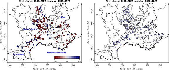
Figure 1. % of change in mean annual maxima between 1960 and 2020 predicted by the non-stationary GEV models using data from (left) 1958–1972, (right) 1958–2020. For readability, the colorscale of the left map is restricted to ±100% (the actual range exceeds ±200%).
Download figure:
Standard image High-resolution imageDaily rainfall data are acquired by Météo-France. About 1500 daily stations are located in this area but with various lengths of observation. We consider 180 stations featuring at least 60 observed years over the period 1958–2020 and we extract, at each station, the series of annual maxima. The stations are relatively homogeneously spread over the region, with however a larger density along the Massif Central flank (see figure 1).
Trend in the statistics of extreme precipitation is assessed by fitting a non-stationary generalized extreme value (GEV) distribution with cumulative distribution function at year t:
where rt
is the annual maximum of a given station,  ,
,  and ξ are the location, scale and shape parameters at year t. We consider linearly varying location and scale parameters:
  ,
,  . This implies that the mean (mt
) and T year return levels (
. This implies that the mean (mt
) and T year return levels ( ) are assumed to vary linearly with years:
where Γ is the Gamma function. This model might not be the most parcimonious (Blanchet et al 2021a) and this could, e.g. affect significance testing but this is out of concern here since we are only interested in trend values.
The GEV model of equation (1) is fitted by maximum likelihood (Coles 2001) at either station. We consider incremental windows, first estimating the model based on the maxima for 1958–1972, then increasing the window size by 1 year (1958–1973), and so on up to the maximal window 1958–2020. Thus 49 GEV distribution estimates are obtained for each station, each estimation being based on 15 (1958–1972) to 63 (1958–2020) maxima.
Since our interest is to assess the instrumental agreement as time goes on, we compare the predicted changes (in mean or return level) for a common period, which is here arbitrarily chosen as 1960–2020. This is given by  and
and  with mt
and
with mt
and  given by equations (2) and (3). Note that this implies extrapolating in time all models (but the maximal one) till 2020 but this is mathematically-speaking no issue since equations (2) and (3) are parametric functions (so we only have to replace t by 2020 therein).
We call the 'consensus curve' the curve defined by the station median of the predicted changes versus time (i.e. versus the window size). Our goal is the assess whether the consensus curve for the mean or return level converges at some point to a nonzero value, i.e. to estimate the time in the past when an agreement has emerged between most stations to point toward a trend. This definition of emergence based on convergence over incremental windows differs from other studies such as Giorgi and Bi (2009), Tramblay and Somot (2018) that assess the TOE based on full series of climate simulations (e.g. from 1950 to 2100). Our TOE can actually be understood as a time when a consensus is reached.
3. Results
For illustration, we show in figure 1 the spatial distribution of the % of change in mean annual maxima between 1960 and 2020 predicted by the non-stationary GEV models using data from either 1958–1972, or 1958–2020. The % of change using 15 years of data are very chaotic, with changes varying from −100% to +100% in few km. When using 63 years, changes are smaller in absolute value but much more homogeneous and very mainly positive.
Figure 2 summarizes such maps by showing the boxplots of % of change between 1960 and 2020 obtained over all incremental windows. The horizontal dashed red line shows a rough estimation of the expected Clausius–Clapeyron response, obtained by combining the Clausius–Clapeyron rate of +6.8% K−1 with the observed annual mean warming over the region of about +1.79 K (Ribes et al 2019), giving an expected increase in extremes of about 12.2% between 1960 and 2020. Note that the expected Clausius–Clapeyron response is an horizontal line in figure 2 because the plots show changes with respect to a common reference period 1960–2020 and hence to a common level of warming. The figure shows that the dispersion of predicted percentage of change between 1960 and 2020 has evolved considerably over time. The data series have indeed become longer over time, gradually covering a period where climate change gets increasingly clearer.

Figure 2. Boxplots of the % of change between 1960 and 2020 predicted over incremental windows. Left: mean maxima. Right: 20 year return level. The expected Clausius–Clapeyron response is shown in dashed red. The black curves show the consensus curves represented by the median of the station estimates as the window increments. The bottom and top of the boxes are the lower and upper quartiles. The upper whisker extends to the largest value no further than 1.5 times the IQR from the boxes. The lower whisker extends to the smallest value at most 1.5 times the IQR from the boxes. The points show the values beyond the end of the whiskers.
Download figure:
Standard image High-resolution imageThree periods stand out in the 'consensus' of the rain gauges. Until the mid-1980s, the rain gauges gave widely varying opinions. Many of them predicted a decrease in extreme between 1960 and 2020 in proportions ranging from 0% to 100%. The data series available—a mere 20 years or so—was too short to produce reliable statistics. Clearly, the change was not yet perceptible in the Mediterranean region at that time. In the 1990s, a dramatic shift occurred. The divergence of predicted changes between rain gauges was halved as a result of longer observation times. More importantly, the vast majority of rain gauges fell into the same intensification opinion. Since the 2000s, this unanimity has been stable. More than 80% of the rain gauges predict an increase. This increase tends to tighten around about 18% for the mean annual maximum and 22% for the 20 year return level. The latter implies that the 20 year return period of precipitation in 1960 turns out to become a 8 year return period of precipitation in 2020. Furthermore 75% of the rain gauges exhibit super-Clausius–Clapeyron behavior (i.e. an increase larger than the expected Clausius–Clapeyron response), which is in coherence with Ribes et al (2019). In view of these analyses, the intensification of exceptional heavy rainfall appears to be undeniable in the region of interest, and has been for a good 10 years. The stabilization of the consensus curve in figure 2 argues in favor of a TOE around 1995–2000, which is quite consistent with the break date of 1985 identified in the region (Blanchet et al 2018, 2021b). This is also consistent with the TOE estimated between 1980 and 2000 is the region in Tramblay and Somot (2018) using climate simulations up to 2100.
The consensus curve—and thus the TOE—vary very little whether they are defined from the mean maxima or from the 100 year return levels, as they corresponds to % of changes rather than absolute changes (figure 3). It can also be noted that, although based on convergence of medians, the TOE defined from the consensus curve corresponds to the time when more than two third of the stations agree on positive trends, whatever the return period considered (figure 3).
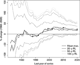
Figure 3. Median (consensus curve) and 75% confidence interval of the % of change between 1960 and 2020 predicted over incremental windows, for the mean maxima, the 20, 50 and 100 year return levels. The black points show the years 1988, 1992, 1999, 2002, 2010, 2020 during which flash-flood events occurred in the region.
Download figure:
Standard image High-resolution imageAnother remarkable property of the consensus curve is to be little sensitive to the occurrence of major events, such as in October 1988 (Nîmes disaster, Duclos et al 1991), 1992 (Ouvèze River, Sénési et al 1996), 1999 (Aude River, Gaume et al 2004), 2002 (Gard River, Delrieu et al 2005), 2010 (Argens River, Ruin et al 2014). The consensus curves obtained by omitting either of these years in the data (i.e. by setting the maxima values of these years to NA) yields to differences no larger than 5% for the mean maxima and no larger than 6% for the 20 year return levels. Another remarkable property of the consensus curve is to be little sensitive to the spatial distribution of the stations since it is based on the median.
In order to illustrate the respective effects of a stationary noise N and a multi-decadal signal S on the presented statistics, we made a simulation exercise. We simulated, at each gauge, n fictitious annual maximum series drawn independently from GEV distributions with either the same stationary parameters as the rain gauges, or non-stationary parameters. In the latter case, the four GEV non-stationary parameters are set so that: (a) the average GEV means and variances over 1958–2020 are equal to the empirical means and variances of gauge readings, (b) the percentages of change in mean and 20 year return level are equal to the median values of the percentage of change of the rain gauges obtained over the maximal window (i.e. corresponding to the abscissa 2020 in figure 2).
Figure 4 compares the incremental medians and interquartile ranges (IQR) predicted from both the simulated data ( runs each) and the observed maxima. The median of the non-stationary series are, as expected, very close to the rain gauge value in 2020, despite a small bias (slight underestimation of the mean and slight overestimation of the 20 year return level). The median of the stationary series converges to 0, as also expected. It can be noted that, even in this idealized experiment, uncertainty in changes is considerable for the smallest windows: the change in mean maxima (resp. 20 year return levels) varies by ±20% (resp. ±50%) around the true value for the 1950–1972 window. Although the nonstationary GEV framework makes it possible to calculate trends regardless of the length of the series, it is clear that estimates over less than 30 years—say—are unreliable even for the mean maxima. Uncertainty obviously decreases as the window increments, going down to ±2% for the mean maxima and ±3% for the 20 year return level with the largest window of 63 years. Differences between the stationary and the non-stationary series are notable—the 95% confidence intervals of the mean and 20 year return level do not overlap when more than 33 years are considered (i.e. using series extending to 1990 or later). The IQR with either the data or the simulations are very similar and super-exponentially decreasing as the series length increases (note the log-scale in the IQR plots of figure 4). Thus the decreasing variability in the boxplots of figure 2 is merely a question of data length. Notably, multi-decadal variability of about 20 years is visible in the median changes based on the data (light gray curve in figure 4), whereas the simulations show more random variability. We note that taking a growing size window shows two main advantages over the fixed (e.g. 20 year) window approach. First it takes the best of the available information at each time step and second it shows the progressive filtering of multi-decadal variability.

Figure 4. Median (consensus curve, top) and IQR in log-scale (bottom) of the % of change between 1960 and 2020 predicted over incremental windows based on either the data (black) or stationary simulations (red), or non-stationary simulations (blue). Left: mean maxima. Right: 20 year return level. The dotted lines show the 95% confidence intervals obtained over 100 runs. The light gray curve shows the cubic smoothing spline fitted to the median series of the data.
Download figure:
Standard image High-resolution image
4. Conclusion
We have used a consensus approach to show the emergence in the 2000s of an agreement between rain gauges pointing toward an increase in extreme daily precipitation in the French Mediterranean Region since 1960. We have shown that the stations agree to an increase of about 18% in mean maximum precipitation in the region and of about 22% in the 20 year return level, which is considerably larger than the 12% increase expected by Clausius–Clapeyron relationship, but it is coherent with previous studies in the region. We have highlighted that the consensus approach shows various benefits, among which it makes the best used of the available data, it is easy to implement, it is robust to the occurrence of major events without requiring regional methods (Blanchet et al 2021a), it is by construction little sensitive to the spatial spreading of the rain gauges, it allows progressive filtering of the multi-decadal variability.
Acknowledgments
This work is part of a collaboration between the University Grenoble Alpes and Grenoble Alpes Métropole, the Metropolitan authority of Grenoble conurbation (deliberation 12 of the Metropolitan Council of 27 May 2016). Part of this work was funded by the IND-EX project with the support of the Rhône Alpes Region in France. The data used in this paper are maintained by MétéoFrance. They can be downloaded under research agreement from the website: http://publitheque.meteo.fr/
Data availability statement
The data that support the findings of this study are available upon reasonable request from the authors.