2.1 Data collection

We acquired 26 radar profiles with the AWI airborne radio-echo sounding (RES) system operated on the Basler BT-67 aircraft Polar6 (Wesche et al., 2016) during the 2016/17 Antarctic season. The radar survey was conducted from a temporary camp (79^∘ S, 30^∘ E) 290 km southwest from the DF station. Survey lines have parallel line spacing of 10 km in the northern part of the study area and 15 km line spacing in the southern part with smaller spacing distances when approaching and leaving the camp (Karlsson et al., 2018). Of the 26 profiles available we analyze 22 with lengths varying from 622 to 898 km. The study area covers a region of about 270 000 km² and an elevation range of about 3400–3810 m (Fig. 1). In this region, ice surface velocities range from 0 to 9.2 m a⁻¹.

The AWI RES system transmits radar waves with a center frequency of 150 MHz, a band width of 20 MHz and an amplitude of 1.6 kW. During the survey it effectively operated as a pulse-limited radar with the 600 ns wide pulse. The theoretical vertical resolution in ice for the 600 ns burst is 50 m (Nixdorf et al., 1999). In this study we use radar returns of the 600 ns long burst from internal reflection horizons (IRHs), as well as from the ice–bedrock interface. The raw radar data have a mean spacing of 5 m along the flight line (which varies with real speed and direction of aircraft) and are sampled at a time interval of 4 ns (Karlsson et al., 2018).

Before picking the IRHs and the ice–bed interface, the radar data are resampled to 12 ns and stacked 7-fold, which leads to a mean trace spacing of ∼ 35 m. In addition, a low-pass filter and a running average filter are used to decrease noise. Automatic gain control (AGC) is used to balance the gain and facilitate horizon tracing. Processing is performed in the seismic environment of the Echos software from Paradigm Geophysical.

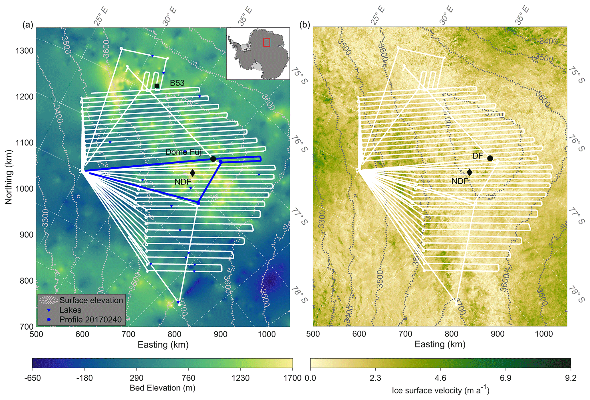
Figure 1(a) Study area in the DF region, with inset showing the position in Antarctica. The white lines represent the radar survey profiles used in our study. The blue line shows the example profile 20170240. We use surface elevation (contour map) and bed elevation from Morlighem et al. (2020) and Morlighem (2022). Subglacial lakes were identified by Karlsson et al. (2018). (b) Ice surface velocities (Rignot et al., 2017, 2011; Mouginot et al., 2012, 2017).

2.2 Horizon picking and dating

In order to provide age markers (i.e., the age of IRHs) and ice thickness to use as constraints in our 1-D flow model, IRHs are traced in the two-way travel time (TWT) domain. The surface reflection is picked automatically in the program Echos and then subtracted in all traces to shift the first break of the radar data to time zero. The maximum reflection power of IRHs is traced manually in the seismic software package “Section”, which allows IRHs to be continuously traced in different radar profiles through intersections between profiles. This ensures that the same isochronous horizons are traced. We trace six (H1, H2, H4–H7) or seven (H1–H7) relatively distinct and continuous IRHs in the radar profiles, since the third IRH, H3, is not clear and continuous enough to be traced in some profiles. Ice–bed returns were picked by Karlsson et al. (2018) through semiautomatic detection routines in MATLAB. These ice thickness data are available on Pangaea (Eisen et al., 2020). The ice–bed returns are often diffuse, especially around mountain peaks, which results in disagreements when using different methods to trace ice–bed returns and thus in differences in ice thickness and modeling results. We emphasize that Karlsson et al. (2018) picked the first (uppermost) ice–bed return when there were uncertainties, so ice thickness estimates can be considered a minimum ice thickness in some places.

TWT is converted to depth assuming a constant radar wave speed of 168.5 m µs⁻¹ in ice (Winter et al., 2017; Lilien et al., 2021) and a 15.5 m firn correction calculated from the depth–density curve in the B53 ice core. The B53 ice core was drilled to 202 m depth by the AWI team during the survey period and is located at 79^∘47^′38^′′ S, 31^∘54^′19^′′ E and ∼ 203.5 km away from the DF drill site (Fig. 1). The point of closest approach to the DF drill site on our radar profiles is located 91.1 m away, at 77^∘19^′ S, 39^∘41^′59^′′ E, on the profile 20170240. Ice thickness at this nearest point observed in the radargram is about 3045 m, and the ice thickness at the DF drill site interpolated between our radar observations is about 3050 m. This agrees with the uncertainty estimates with a previously inferred ice thickness of 3028 ± 15 m from a radar observation (Fujita et al., 1999), and it approximates the depth of the second DF deep ice core, 3035.2 m, which is considered to be very close to the ice–bed interface (Motoyama, 2007).

IRHs at this location closest to the DF drill site are firstly converted to depth and then dated by vertical interpolation of the ages from the DFO-2006+AICC2012 timescale (Dome Fuji Ice Core Project Members, 2017), available to a depth of 3031 m with an ice age of 715.9 kyr BP, and finally transferred to the radargram at the depths of the IRHs. Figure 2 shows traced IRHs H1–H7 in the profile 20170240 with the point of closest approach shown as the vertical white line. The ages of IRHs, ranging from 31.4 ka (H1) to 169.1 ka (H7), and their age uncertainties are marked in Fig. 2. Ages of different IRHs are then transferred to all profiles via our network, which then serve as the primary constraint on the 1-D model.

2.3 Age uncertainty of internal reflection horizons

The uncertainty of IRH age estimates directly impacts the reliability of the results from the model, and it includes uncertainty of the ice-core age scale and age uncertainty caused by depth uncertainty of IRHs. For the depth uncertainty of IRHs, we consider slope-induced uncertainties caused by the offset of the closest radargram to the DF drill site, as well as the uncertainties caused by the firn correction, the dielectric constant of ice and the precision of the range estimate in determining depth (Cavitte et al., 2016).

The slope of each IRH varies from 1 to 14.7 m km⁻¹, which results in a corresponding uncertainty from 0.1 to 1.5 m for the 91.1 m offset (the distance between the DF drill site and the point of closest approach on the radar profile). For the firn correction, we used the AWI's Ice-CT system to measure the density–depth profile in the upper 126 m of the B53 ice core, with an observational error up to 1 % (Freitag et al., 2013). This results in an uncertainty of 0.5 m in the firn correction. The depth uncertainty of the dielectric constant affected by anisotropy and temperature is taken to be 1 % (Lilien et al., 2021).

The precision of the range estimate is determined by the pulse width of the radar waveform, the signal-to-noise ratio (SNR) and the sub-resolution reflector fluctuations, and it is always numerically smaller than the vertical resolution. The last term could be ignored when the reflectors display a continuity in reflection amplitudes and consequently traceability (Cavitte et al., 2016). In our case the precision of the range estimate is almost the same as the range resolution (∼ 25 m), but it is actually lower (> 25 m) in the deep ice, since our radar system has a 600 ns pulse width. The resolution of our system is lower than that of more advanced radar systems, and this causes a smaller number of internal horizons, as well as a lower traceability. Moreover, the bedrock topography is characterized by a series of mountain ranges and valleys and a wide melting distribution in the DF region, which lead to the discontinuity of isochrones at some places, especially near the bottom. Therefore, we need to consider the sub-resolution of different reflectors in our analysis.

We find that the uncertainty caused by the low traceability and continuity is large when we trace the horizons manually. We therefore attempt to trace horizons via several paths to circumvent locations where horizons are disturbed or discontinuous. Therefore, our best guess for the uncertainty of each IRH depth is based on continuity and definition during manual tracing. It varies from 20 to 50 m.

The overall depth uncertainty varies from 28.5 to 70.5 m, leading to an age uncertainty range from 2.1 to 16.8 ka. The age uncertainty of the ice core itself is interpolated from the age errors in the age scale DFO-2006 (Kawamura et al., 2007). In total, the age uncertainties range from 3.0 to 19.0 ka for the seven IRHs.

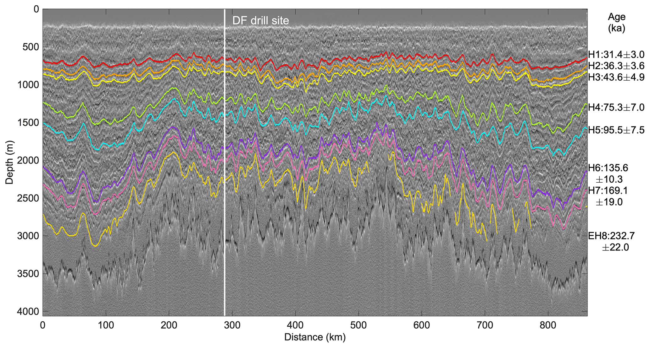
Figure 2Radargram of the profile 20170240. The vertical white line shows the location of the DF drill site. Lines with different colors represent continuous horizons H1–H7 and the specially traced discontinuous horizon EH8. The dated age and age uncertainty of each horizon is marked on the right.

Download

2.4 The 1-D age model

To extrapolate the age–depth profile in the study area below the depth of the deepest IRH, we use a 1-D pseudo-steady ice flow model developed by Parrenin et al. (2006, 2017) but with simplified constraints. This model assumes that the geometry, the shape of the vertical velocity profile and the relative density profile are constant. The real ice age χ can be calculated using the steady age $\overline{\mathit{\chi }}$ and the temporal factor r(t) by

where r(t) is deduced from the accumulation record of the DF ice core. We assume r(t)=1 beyond the extent of the DF ice-core record (715 kyr BP), otherwise

where $\dot{a}$ is the accumulation rate and $\overline{a}\left(x\right)$ is the temporally averaged accumulation rate at a certain point x. The steady age $\overline{\mathit{\chi }}$ can be inferred from depth d and the layer thickness λ(d):

Assuming that there is no basal melt, λ(d), approximated by the Lliboutry model (Lliboutry, 1979), is

where p is a shape factor controlling vertical deformation (Lilien et al., 2021), H_m is the mechanical ice thickness, which is different from the observed ice thickness H_obs. The main difference between the model we use here and the one developed by Parrenin et al. (2006) is that no thermal modeling and thermal boundary conditions are considered here. Instead, we use the inferred H_m to judge if melting is present or if stagnant (i.e., dynamically irrelevant) ice prevails. When H_m is greater than the observed ice thickness H_obs, we have melting conditions at the base. Otherwise, there is stagnant ice. If there is basal ice melting, the melt rate m can be obtained by

We use a SciPy least-square optimization to deduce the age–depth profile by varying $\overline{a}$, $H_{\mathrm{m}}^{\prime }$ and p^′, where $H_{\mathrm{m}}=e^{H_{\mathrm{m}}^{\prime }}$ and $p=e^{p^{\prime }-\mathrm{1}}$ to prevent $p<-\mathrm{1}$ and H_m<0. The minimized cost function is

where i is the ordinal number of the IRH, χ^iso is age of the IRH, σ^iso is the confidence interval on the age, χ^mod is modeled age and d^iso is the depth of the IRH, with p_prior=3 and ${\mathit{\sigma }}^{p^{\prime }}=\mathrm{1}$ (Parrenin et al., 2007; Chung et al., 2023). The uncertainty of each inverted parameter could be inferred from the optimization and the covariance matrix. To quantify the reliability of the model at each point, we introduced a reliability index σ_R, i.e., the standard deviation of residuals:

where n_iso is the number of IRHs, and R is the residuals deduced by

In this way the model achieves the balance of efficiency and numerical requirements. More details on the model can also be found in the companion paper (Chung et al., 2023).

3.1 Modeling results for an example profile

We integrate 1-D modeling results every 1 km along the example profile 20170240, displayed as a cross section through the ice sheet in Fig. 3, to get the 2-D modeled age–depth distribution. We find ice older than 1 Ma along the profile from ∼ 150 to ∼ 550 km, where the ice sheet is thinner than in the other parts. Basal melting is present at the DF drill site and along most parts of the profile, where the mechanical ice thickness H_m (dashed purple line) is larger (deeper) than the observed ice thickness (black line).

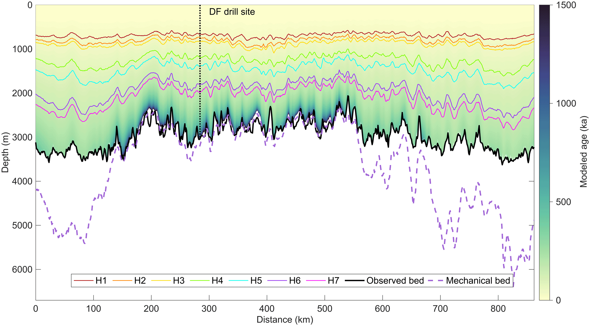
Figure 3Modeled age–depth distribution of the radar profile 20170240. The colored lines (see legend) correspond to the traced IRHs shown in Fig. 2. The dashed purple line shows the mechanical ice thickness H_m, and the black line shows the bed observed in the radargram. Where the dashed purple line is above the black line, stagnant ice is present and the depth difference between the two lines is the thickness of the stagnant-ice layer. In other cases, melting prevails.

Download

3.2 Age of basal ice

We use 20 kyr m⁻¹ as a cutoff value for age density of basal ice, beyond which the usage of proxies in the ice for paleoclimate reconstruction is currently difficult. This age density corresponds to a full 40 kyr climate glacial–interglacial cycle in 2 m of ice. Figure 4a shows the age of basal ice (i.e., at the depth of the bed or where the age density reaches 20 kyr m⁻¹) in the DF region. It varies from 220 to 2530 ka. Figure 4b shows the corresponding depth of the basal ice, which falls in a depth range of 1.6–3.8 km. The age of basal ice at the DF drill site is extrapolated as 1350 ± 500 ka at the ice–bed interface. The maximum age of ice at NDF is extrapolated as 1470 ± 510 ka at a depth of 2081 m. Figure 4c shows the age uncertainty of the basal ice, which ranges from 30 to 1050 ka and varies with the age of basal ice.

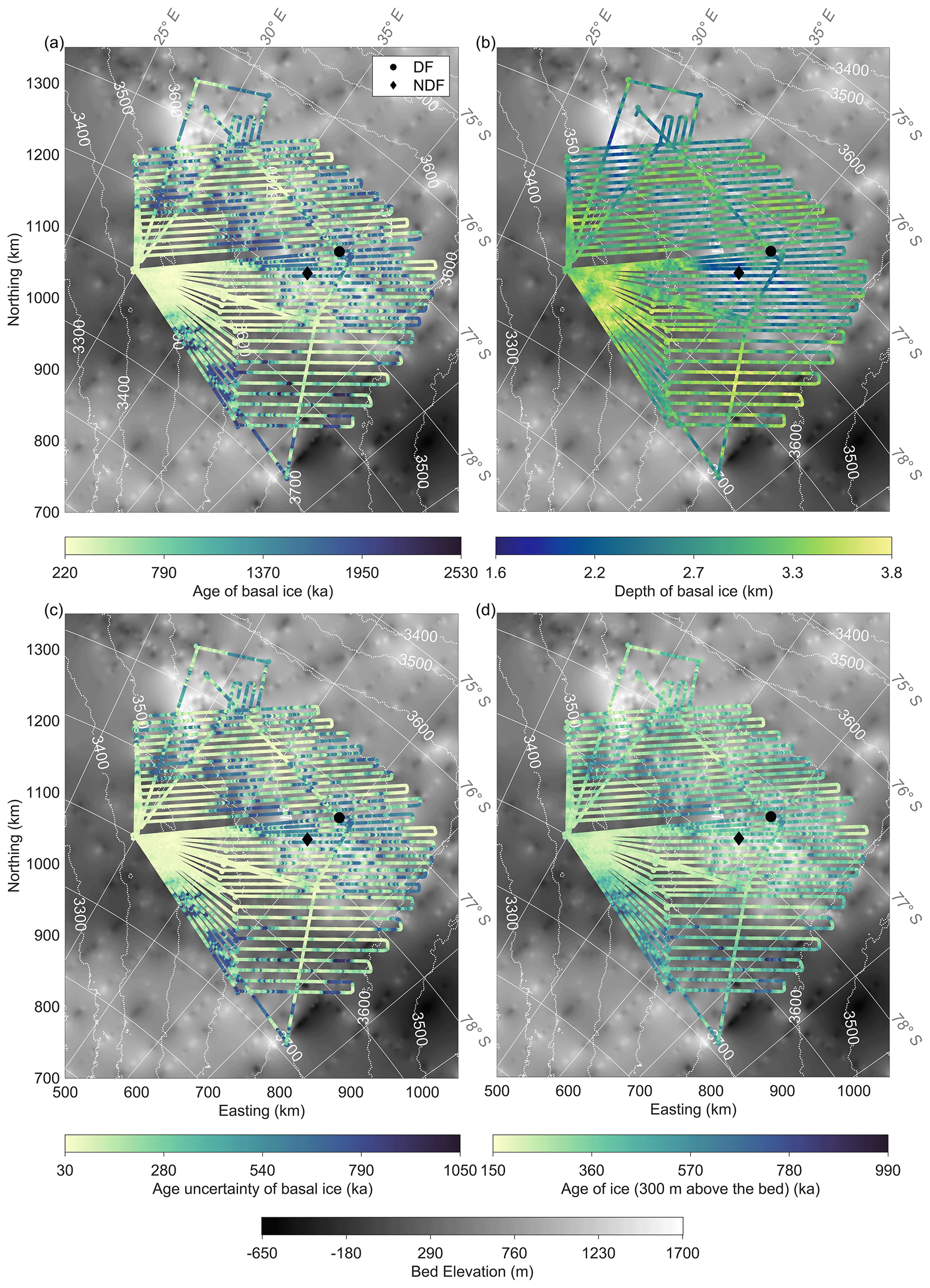
Figure 4(a) Modeled age of basal ice at a maximum age density of 20 kyr m⁻¹. (b) Depth of the basal ice at a maximum age density of 20 kyr m⁻¹. (c) Modeled age uncertainty of the basal ice. (d) Modeled age of the ice at a height of 300 m above the bed.

Download

The age density of ice at 1.5 Ma is shown in Fig. 5a, with a range of 6–20 kyr m⁻¹. It is considered sufficient for paleoclimatic reconstructions (Fischer et al., 2013). This figure also points out the four candidate areas where ice of more than 1.5 Myr old could potentially be found (marked as dashed dark red ellipses): the first one is a large subglacial mountain range located within a ∼ 100 km radius around the DF drill site; the second one is ∼ 160 km to the west of the DF drill site, connected with the first site; the third one is ∼ 240 km to the west of the DF drill site; and the fourth one is ∼ 260 km to the south of the DF drill site. These four potential candidate areas are all situated in regions with an ice thickness of 2200–3000 m, where the ice is not too thick, which would result in basal melting, but still thick enough to potentially contain a long-term and sufficiently resolved ice-core record. Moreover, these sites, especially the first one close to DF, appear to be distributed over high plateaus. This could imply that the ice column here is potentially less disturbed and includes horizons of higher lateral continuity.

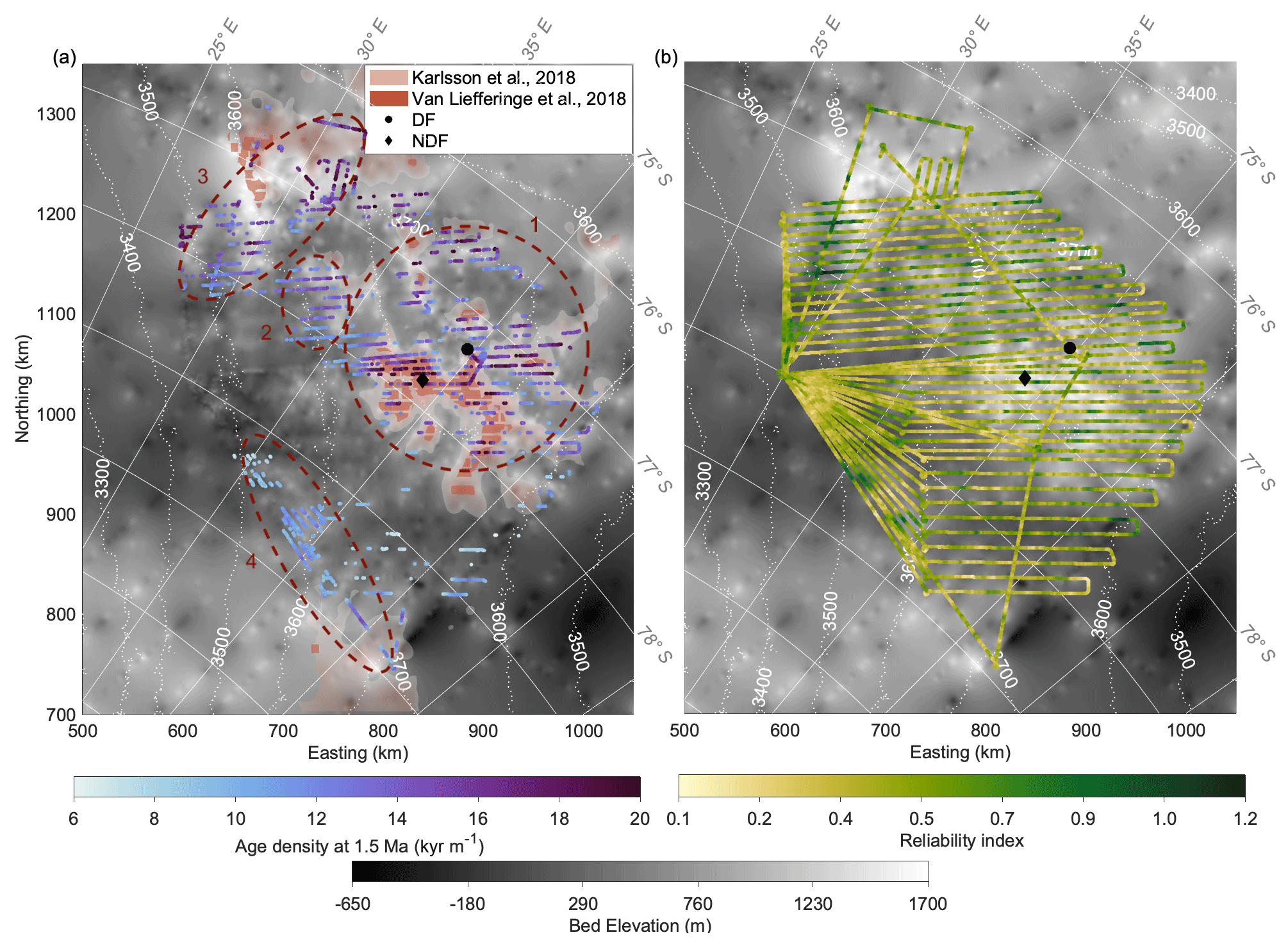
Figure 5(a) Age density of ice at 1.5 Ma: the dark red ellipses show the potential old sites considering basal age and age density. Semi-transparent pinkish-red-colored shades show potential old-ice sites suggested by Karlsson et al. (2018) – the deeper the color, the higher the possibility of old ice. The orange shades show the old-ice sites suggested by Van Liefferinge et al. (2018). (b) Reliability index (σ_R) map in the DF region: the reliability of the model output decreases with decreasing reliability index (σ_R) increasing.

3.3 Basal thermal states

Basal conditions are crucial criteria for the presence of old ice because any melting causes ice loss in the lowermost part of the ice column, which severely limits the age of basal ice (Fischer et al., 2013). From our model we also obtain the basal conditions, including melt rate or stagnant-ice thickness (Fig. 6a). According to our results, basal melting prevails over frozen conditions with the formation of stagnant ice in the survey area. Modeled basal melt rates vary from 0 to 8.4 mm a⁻¹. Melting is significant ∼ 200 km southwest and ∼ 150 km southeast of DF, where we observe ice thicker than 3000 m, i.e., ice thick enough for the temperature to reach the pressure melting point. The basal melt rate at the DF drill site is interpolated as 0.1 ± 0.4 mm a⁻¹.

Stagnant ice has a thickness range of 0–410 m. Two clusters of stagnant ice are distributed ∼ 60 km southwest (immediately around NDF) and ∼ 180 km west of DF (in the second old-ice candidate site). The thickness of stagnant ice is modeled as 207 m at NDF. Our results show that melt rates are generally higher in subglacial basins and lower (or even frozen conditions) in subglacial mountainous terrain.

3.4 Accumulation rate

Accumulation rate is another important factor for the age distribution. We show the temporally averaged (over 720 kyr) accumulation rates in the DF region from our model results in Fig. 6b. They vary from 0.015 to 0.038 m a⁻¹ ice equivalent. At the DF drill site, the accumulation rate spatially interpolated between the radar lines is 0.022 m a⁻¹. In the larger DF region, it shows a west–east decreasing gradient. In the Supplement Fig. S1 we also show the shape factor map in the DF region obtained from the model.

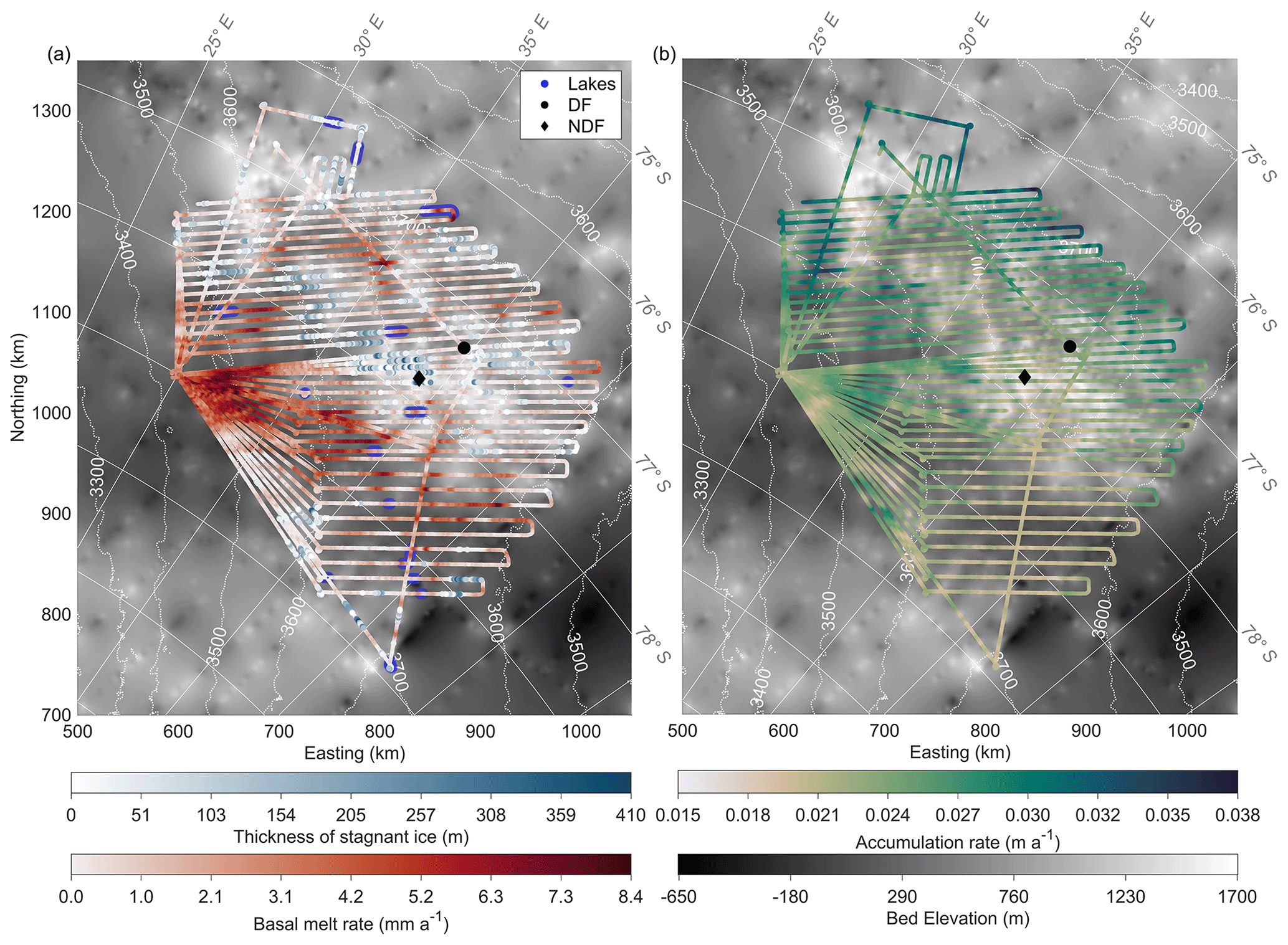
Figure 6(a) Modeled stagnant-ice thickness and basal melt rate along the profiles of the radar survey: blue represents stagnant-ice thickness, and red represents the melt rate. Dark blue lines are subglacial lakes deduced from basal reflectivity in radargrams by Karlsson et al. (2018). (b) Modeled averaged accumulation rate in ice equivalent along the profiles of the radar survey.

4.1 Age of ice: comparison with previous studies

There is significant uncertainty in the basal age of ice over the entire DF region. We relate this phenomenon to the fact that the number and depth of IRHs used as constraints for the model are limited by their traceability in our radar data set. IRH constraints help to determine the shape of the thinning function (p factor); therefore, using more IRHs gives a more accurate p value. The thinning function is almost linear in the upper section of the ice sheet and then becomes nonlinear in the deepest part. Since the IRHs we have traced are located in the top two-thirds of the total ice thickness, we cannot constrain the model well in the lower one-third. However, this lower section has the largest impact on the p value. For comparison, in the Dome C region, the age uncertainty of each IRH is similar to that in the DF region, and Chung et al. (2023) adapted the same model approach, but the modeled age uncertainty of basal ice is much smaller in the Dome C region. This is likely due to more IRH constraints covering a larger portion of the ice sheet thickness in the DC region. We consider this comparison important, as the same approach applied in different regions and/or to a different radar data set can yield a considerably different uncertainty.

Several previous studies have already investigated the potential age of basal ice either at the DF drill site or in its surrounding region. At the DF drill site, Parrenin et al. (2007) proposed that ice more than a million years old could exist near the ice–bed interface, according to the results of their 1-D ice flow model. Hondoh et al. (2002) deduced chronologies of the DF ice core based on the correlation between the local metronomic signal (Milankovitch components of the past surface temperature oscillations) and the isotope record. They then extrapolated this timescale to 3050 m depth using a simplified ice flow model. Their result suggested that the age may reach 2000 ka at about 3000 m depth at the DF drill site. These two results agree approximately with the range of our inferred bottom age of 1350 ± 500 ka at the ice–bed interface (∼ 3050 m).

Obase et al. (2023) used a 1-D ice flow model, which computes the temporal evolution of the vertical age and temperature profiles. They also extended their modeling results along a DF–NDF radar transect from DF to NDF, where the basal ice has a tendency to be older. They used ground-based radar data from the JARE59 (59th Japanese Antarctic Research Expedition) survey (2017–2018) which covered an area of approximately 120 km × 100 km with a dense grid of radar lines. The data were collected using an incoherent pulse-modulated VHF radar sounder with a peak transmission power of 1 kW and transmitter pulse widths of 60 and 250 ns, which corresponds to a pulse-limited vertical resolution of 5 and 21 m, respectively. In addition, their model is transient; therefore, age and temperature both change with time. It estimates the age through the vertical advection equation and uses the GHF as the basal boundary condition, while we use a 1-D steady model, which calculates the age through an analytical thinning function and excludes all thermal modeling by introducing a mechanical ice thickness.

Despite the differences in the radar data characteristics of the JARE59 and AWI surveys and slightly different models, the results are reasonably consistent. We estimate the age of basal ice at DF to be 1350 ± 500 ka, while Obase et al. (2023) extrapolated it as a range between 400–1000 ka with a GHF in the range of 60–52 mW m⁻², respectively, in their Fig. 6a. In addition, our results confirm that the age of basal ice increases from DF to NDF.

The two previous studies by Karlsson et al. (2018) and Van Liefferinge et al. (2018) are based on a thermodynamic model, considering regions with a surface ice flow velocity lower than 1 m a⁻¹. Their main constraint for the presence of old ice is that the GHF is not sufficiently large to cause temperate conditions at the base and thus melting. Another criterion is ice thicker than 2000 and 2500 m. They suggested several potential areas holding old ice, which are displayed by semi-transparent pink and orange shades in Fig. 5. Our approach, in contrast, is solely based on the observed age–depth distribution, which is then extrapolated to a greater depth by using observed accumulation rates and making assumptions about the thinning function.

The model we are using does not take into account the thermodynamics at all, thus it is more independent of GHF estimates. However, the sites with potentially “old ice” suggested by the above-mentioned two studies show a considerable correspondence in some places with our results, especially at the first candidate in the region with low surface velocity (a large subglacial mountain range located immediately around the DF drill site). We consider that the two main underlying reasons for this consistency are the use of ice thickness in both models, which has implied the important impact of ice thickness on the age distribution of the ice, and the validity of the approximations regarding the thinning function in our approach.

4.2 Basal thermal state and accumulation rate: comparison with previous studies

A spatial comparison between our result and subglacial lakes identified previously by Karlsson et al. (2018) in Fig. 6a shows that all 16 lakes are located in regions where we obtain basal melting, and in 11 lakes we can observe significant melting.

The basal melt rate is a parameter impacted by the spatial distribution of GHF, which is a regional parameter that can also show strong variations on the local scale, depending on topography (Colgan et al., 2021). By averaging the local GHF variations, we calculate regional melt rates in different areas around the DF drill site from our results for the comparison with previous basal melt rates at DF. In our results, the mean basal melt rates increase with distance from the DF site.

Using a 1-D ice flow model at the DF site, Parrenin et al. (2007) suggested that the basal melt rate is < 0.2 mm a⁻¹ with a probability of 90 %. Seddik et al. (2011) deduced a basal melt rate of ∼ 0.35 mm a⁻¹ assuming a GHF of 60 mW m⁻². Obase et al. (2023) suggested that there is no melting at DF for a GHF < 56 mW m⁻² and the melt rate rises to ∼ 0.4 mm a⁻¹ when GHF equals 58 mW m⁻². These three results all agree with our mean basal melt rate of 0.2 ± 0.4 mm a⁻¹ within 5 km around DF.

Obase et al. (2023) also simulated a basal melt rate change from 0.6 to 1.5 mm a⁻¹ for a GHF increasing from 60 to 64 mW m⁻² in their Fig. 5. This agrees with our averaged basal melt rate of 1.4 ± 0.7 mm a⁻¹ within 200 km around the DF site.

Talalay et al. (2020) estimated a basal melt rate of 2.5 ± 0.5 mm a⁻¹ at DF based on the temperature profile measured in the ice-core borehole and an analytical solution to infer the vertical velocity. This value is consistent with our mean basal melt rate of 1.7 ± 0.8 mm a⁻¹ in the entire DF region. However, this value is very different from our estimate at the DF drill site and – despite potential shortcomings in their approach – probably closer to reality. In Sect. 4.3.3 we discuss the possible overestimation of the basal ice age due to an inflection point at the bottom of the timescale, which would mean that we underestimate the basal melting. Figure S2 shows the mean value and standard deviation of the basal melt rates within different distances of the DF drill site.

In the larger DF region, model-derived stagnant ice is only present along 8 % of the radar profiles and has an average thickness of 96 m. The distribution of the stagnant ice implies that the region immediately around NDF is the area most likely to have a cold bed which could hold old ice in the DF region. Our companion paper shows that in the DC and LDC region, the basal thermal states are very different. Stagnant ice prevails over melting in the DC area, and it dominates the LDC region, with a thickness of up to 250 m (Chung et al., 2023). The relatively warm basal thermal condition in the DF region makes it less likely that old ice exists. Complementary to our model results, other studies have found evidence of stagnant ice in radargrams as notable events, e.g., no continuous or coherent reflecting horizons (Lilien et al., 2021) or diffuse scattering (Cavitte, 2017) in radar detection range. However, in the radar data set we use, there is an echo-free zone (EFZ) above the bed, with a thickness of several hundreds of meters. There are various possible causes for an EFZ, e.g., sensitivity of the radar system, deformation, folding or recrystallization of ice (Drews et al., 2009; Franke et al., 2023). We consider that the EFZ in our data set is most likely caused by the performance of the radar system, as in the same region more modern systems can detect somewhat deeper, more coherent horizons (Rodriguez-Morales et al., 2020). Therefore, we could not observe any unambiguous evidence of stagnant ice in our radargrams. Fujita et al. (2012) found no features in their radar observations that could be interpreted as evidence of the refreezing basal water. They attributed this to the smaller variations in bedrock topography and thus ice thickness in the DF area compared to other regions in Antarctica where basal freeze-on was proposed. Basal meltwater would thus more favorably drain downstream in the DF area than follow paths which would enable local freeze-on locally.

In the DF region, Fujita et al. (2011) showed a map of accumulation rate with a decreasing trend from 76 to 78^∘ S, which is consistent with the distribution of accumulation rate in our result.

4.3 Reliability and sensitivity study of the 1-D model

4.3.2 Sensitivity study

We next discuss sensitivity studies with which we investigate how different data inputs and constraints affect the model and how the reliability of the model could be improved.

The thinning function and the normalized age–depth scale have a stronger gradient in deeper ice than at shallower depths. Therefore, the deepest horizon, as well as the underlying age–depth scale, may have an effect on our modeling results, including shape factor p, accumulation rate $\dot{a}$, mechanical ice thickness H_m and age of basal ice χ_b. To investigate these effects, we perform two sensitivity experiments for the profile 20170240.

Our first run corresponds to the standard model run (STD) which we have been discussing so far; i.e., it uses six or seven traced IRHs and DFO-2006+AICC2012 as the timescale. The timescale provides the temporal variations in the accumulation rate at DF and allows us to date the IRHs.

The second model run (RUN II) investigates the impact of using a different number of traced IRHs to constrain the model. In order to give a better constraint, an extra deeper discontinuous eighth horizon, EH8 with an age of 232.7 ka, was traced (Fig. 2). As this IRH is discontinuous in the study region, it could not be used reliably on all other radar profiles, but it still provides a useful addition to those profiles where it is present.

In the third run (RUN III), we analyze how different timescales influence the modeling results. We use IRHs H1–H7 from the standard run as constraints but replace DFO-2006+AICC2012 with DFGT-2006. Parrenin et al. (2007) reconstructed the age from the first DF ice core using a 1-D flow model, referred to as DFGT-2006. Below 2503 m (the depth of the first deep ice core), the temporal variations in accumulation rate could not be as reliably reconstructed in DFGT-2006 as for other ice cores, as it was derived from marine cores. Therefore, to increase reliability, we use the temporal variations in accumulation rate below 2503 m from timescale DFO-2006+AICC2012 as a replacement.

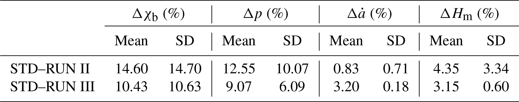
In order to quantify the difference between model results from different runs, we provide statistic values of relative percentage difference in shape factor Δp, accumulation rate $\mathrm{\Delta }\dot{a}$, mechanical ice thickness ΔH_m and age of basal ice Δχ_b along the profile 20170240 between STD and RUN II and STD and RUN III in Table 1. The relative percentage difference between model results from two different runs is

$$\begin{array}{}\text{(9)}& \mathrm{\Delta }X={\displaystyle \frac{|X_{\mathrm{1}}-X_{\mathrm{2}}|}{\mathrm{0.5}(X_{\mathrm{1}}+X_{\mathrm{2}})}},\end{array}$$

where X_i is the model-derived parameter; the index i represents different runs; and X could be p, $\dot{a}$, H_m or χ_b. In the following paragraphs we discuss the results. For extended illustration we refer to the Supplement, where we provide and analyze the model results for all three runs in Fig. S3 and relative percentage difference in model results between STD and RUN II and RUN III in Fig. S4.

The outcome of RUN II shows that the age of basal ice and the shape factor are severely affected by an extra IRH (mean Δp=12.55 % and mean Δχ_b=14.60 %). In some regions, EH8 has a somewhat different shape from the upper seven IRHs and thus changes the inferred shape factor and thinning function of each modeled point, which leads to significant change in the age of basal ice. Between STD and RUN III, the mean relative percentage differences in age of basal ice and the shape factor are also large (10.43 % and 9.07 %). They thus prove the importance of using the most reliable ice-core timescale. The standard deviation of Δp and Δχ_b are significant (6.09 % and 10.63 %), which could be related to the changes in subglacial topography.

The relative percentage difference $\mathrm{\Delta }\dot{a}$ (absolute values) of STD minus RUN II and RUN III has a mean value of 0.83 % and 3.20 %, respectively, which implies the accumulation rate is almost unaffected by adding an extra IRH and is affected more by the timescale. The standard deviation of $\mathrm{\Delta }\dot{a}$ between STD and RUN III is low (0.18 %), which proves that the relative percentage difference seems less variable along the profile. We therefore suggest that using different temporal variations in accumulation rates at DF could be the main reason for the difference in the modeled accumulation rate between STD and RUN III. This is, however, not surprising, as accumulation has a larger influence on isochrones near the surface and a smaller influence on the ones at a greater depth (Sutter et al., 2021).

Mean values of the relative change in the mechanical ice thickness ΔH_m imply that both the number of IRHs (4.35 %) and change in age scale (3.15 %) have a comparatively small impact on the deduced mechanical ice thickness. This implies that the mechanical ice thickness obtained from our model is relatively robust compared to other quantities.

Table 1Mean value and standard deviation of relative percentage difference in age of basal ice Δχ_b, shape function Δp, accumulation rate $\mathrm{\Delta }\dot{a}$ and mechanical ice thickness ΔH_m between model runs for the profile 20170240.

Download Print Version | Download XLSX

4.3.3 Comparison of the age–depth scales

Comparing the age–depth distribution at the DF drill site of the three model runs (Fig. 7), we find that at depths above ∼ 2500 m, the three runs have very similar age–depth scales. The differences between STD and RUN II and RUN III are much larger below a depth of 2500 m, where STD has an age of basal ice of 1350 ± 500 ka. RUN II with an extra horizon results in an age of basal ice of 1960 ± 730 ka, while RUN III uses the input from a different timescale and obtains an age of 1930 ± 770 ka at the basal ice. This comparison shows that both the number of IRHs and the timescale have a significant influence on the age of basal ice. Since RUN III uses the extrapolated timescale (DFGT-2006) and not the timescale of the second DF deep ice core determined by ice-core analysis (DFO-2006+AICC2012), we will not consider it further in the discussion.

If we only focus on the age of basal ice, it seems that both modeled ages (STD and RUN II) deviate from their timescale DFO-2006+AICC2012. The modeled age of STD even seems more reasonable than the modeled age of RUN II with one fewer IRH, although it is important to note that there is huge uncertainty for RUN II and STD. However, since we cannot simply and independently assess the quality of the model results based only on the age of basal ice, we will next analyze the complete age–depth profiles and discuss the age–depth distribution of each run.

Comparing the modeled ages of STD and RUN II with their timescale (DFO-2006+AICC2012), we find that above ∼ 2350 m, both modeling results have good agreement with the timescale. From ∼ 2350 to ∼ 2745 m, only the modeled age of RUN II agrees with the timescale. The STD modeled age is numerically smaller than the age from the timescale, the difference between them increasing with the depth. This finding shows the significant impact of the extra IRH, EH8, in RUN II: with one more IRH which is 257 m deeper and 63.6 kyr older than the one above, the modeled age stays comparatively accurate for a further ∼ 395 m in depth.

RUN II has a reasonable performance down to a depth of ∼ 2745 m, where the age is modeled as 540 kyr BP. This depth is ∼ 300 m above the bed, which is exactly the depth of the inflection point in the timescale DFO-2006+AICC2012. Below this depth, the age–depth profile of the model keeps following the exponential distribution as a model assumption, but the timescale of the ice core shows a curvature reversal. Thus, the modeled age gradient is steeper in the same depth range, which leads to the large overestimation of the age of basal ice by a factor of 2 in this case. Figure 4d depicts the spatial distribution of the age of ice at 300 m above the bed. It provides relatively accurate age values while excluding the lowest part of the ice. The age has a range of 150–990 ka and implies that there is a small area for old ice at this depth ∼ 200 km southeast of DF.

Obase et al. (2023) show this inflection at the same depth (∼ 300 m above the bedrock) in their Fig. 6a, and it also caused a much older modeled age compared to the observation. Such an inflection point in the age–depth scale obviously indicates that the underlying analytical assumption for our model approach is less valid below its depth of occurrence.

A similar phenomenon was also observed in our companion study with the same model approach (Chung et al., 2023) at EPICA Dome C (EDC), though much older IRHs (up to 476.4 kyr BP) were dated there. They pointed out that the modeled age at the deepest dated point for the EDC drill site was around 100–200 kyr older than would be expected from the AICC2012 age–depth profile. The reason could be that the profile of the timescale AICC2012 determined by ice-core analysis does not follow an exponential profile in the lower 200 m of dated ice. Since the timescale of EDC does not change as drastically as that of the DF ice core near the bedrock, the overestimation of the modeled age of basal ice at EDC is not as significant as that at DF. For illustrative purposes we also show the model-derived age–depth scale and AICC2012 timescale at EDC in Supplement Fig. S5.

To solve this overestimation problem in the case of DF, only more continuous isochrones below the inflection point, i.e., the lowest 300 m, would provide better constraint for the model. This is not possible with our radar data set and is also unlikely to be easily achievable in other data sets (e.g., Tsutaki et al., 2022).

The logging of the DF borehole and the drilling process indicated melting at the base of DF (Motoyama et al., 2021), which could be one reason for the inflection point in the timescale of the ice core. This would imply that the significant overestimation likely occurs in areas with basal melting. Given that there is only one deep ice core in the DF region, we lack an additional timescale extending towards the bedrock to prove our hypothesis. Whether the inflection point in the age–depth profile is a general feature in the DF region is still an open question.

Overall, we find that our model works quite well in the upper two-thirds of the ice column according to the calculated reliability index (the standard deviation of the age difference between observation and model results). It also seems appropriate in the deeper part of the ice column at DF, down to the depth of the inflection point of the timescale. Since we have found that areas of basal melting prevail over those with stagnant ice in the DF region, it is possible that an overestimation of age occurs in the deep ice at various places, as has already been observed at DF. Taking this into consideration, we emphasize the importance of considering the basal thermal state for locating old ice: i.e., more attention should be paid to areas indicating the presence of stagnant ice.

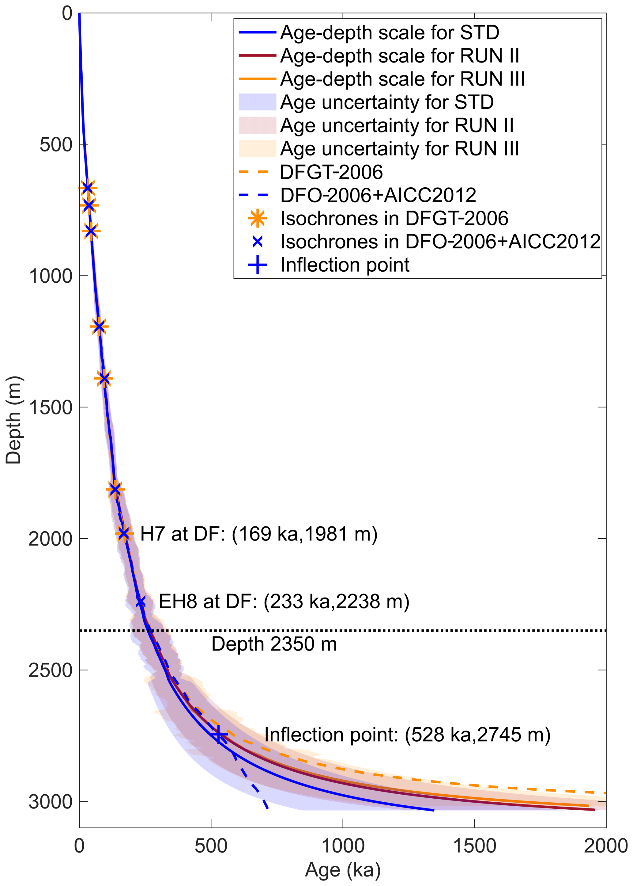
Figure 7Comparison of age–depth scales of three runs (solid lines), their uncertainties (shades) and two timescales from the DF ice core (dashed line). Note that the uncertainties of RUN II and RUN III are similar, so their shades are mostly overlapping. The asterisks and crosses show the age and depth of IRHs for the DFGT-2006 and DFO-2006+AICC2012 timescales, respectively. The plus sign shows the inflection point of the timescale DFO-2006+AICC2012. Labels at the distribution indicate horizon, age and depth.

Download

4.4 Limitations of radar system and model

In the following we will discuss the current limitations from the perspectives of the radar system and the model, respectively, in order to point out potential improvements for future approaches.