Article

Modeling Land Surface Fluxes from Uncertain Rainfall: A Case Study in the Sahel with Field-Driven Stochastic Rainfields

by
Bernard Cappelaere
1,*,
Denis Feurer
1,2,
Théo Vischel
3,
Catherine Ottlé
4,
Hassane Bil-Assanou Issoufou
5,
Stéphane Saux-Picart
6,
Ibrahim Maïnassara
1,7,
Monique Oï
1,
Jean-Philippe Chazarin
1,
Hélène Barral
1,
Benoit Coudert
8 and
Jérôme Demarty
1
1
HydroSciences Montpellier (HSM), University Montpellier, CNRS, IRD, 300 av. Emile Jeanbrau, 34090 Montpellier, France
2
LISAH, University Montpellier, INRA, IRD, Montpellier SupAgro, 2 Place Viala, 34060 Montpellier, France
3
IGE, University Grenoble Alpes, CNRS, Grenoble INP, IRD, 38058 Grenoble, France
4
LSCE/IPSL, CNRS-CEA-UVSQ, University Paris-Saclay, 91191 Gif-sur-Yvette, France
5
Départment Sciences et Techniques de Productions Végétales, University Dan Dicko Dankoulodo, Maradi BP 465, Niger
6
Centre National de la Recherche Météorologique (CNRM), Université de Toulouse, Météo-France, 22300 Lannion, France
7
IRD, 276, Av. de Maradi, Niamey BP 11416, Niger
8
Centre d’Études Spatiales de la Biosphère UMR 5126, Université de Toulouse, 31400 Toulouse, France
*
Author to whom correspondence should be addressed.
Atmosphere 2020, 11(5), 465; https://doi.org/10.3390/atmos11050465
Submission received: 11 October 2019 / Revised: 31 March 2020 / Accepted: 27 April 2020 / Published: 4 May 2020
(This article belongs to the Special Issue Evapotranspiration Observation and Prediction: Uncertainty Analysis)

Abstract

:
In distributed land surface modeling (LSM) studies, uncertainty in the rainfields that are used to force models is a major source of error in predicted land surface response variables. This is particularly true for applications in the African Sahel region, where weak knowledge of highly time/space-variable convective rainfall in a poorly monitored region is a considerable obstacle to such developments. In this study, we used a field-based stochastic rainfield generator to analyze the propagation of the rainfall uncertainty through a distributed land surface model simulating water and energy fluxes in Sahelian ecosystems. Ensemble time/space rainfields were generated from field observations of the local AMMA-CATCH-Niger recording raingauge network. The rainfields were then used to force the SEtHyS-Savannah LSM, yielding an ensemble of time/space simulated fluxes. Through informative graphical representations and innovative diagnosis metrics, these outputs were analyzed to separate the different components of flux variability, among which was the uncertainty represented by ensemble-wise variability. Scale dependence was analyzed for each flux type in the water and energy budgets, producing a comprehensive picture of uncertainty propagation for the various flux types, with its relationship to intrinsic space/time flux variability. The study was performed over a 2530 km2 domain over six months, covering an entire monsoon season and the subsequent dry-down, using a kilometer/daily base resolution of analysis. The newly introduced dimensionless uncertainty measure, called the uncertainty coefficient, proved to be more effective in describing uncertainty patterns and relationships than a more classical measure based on variance fractions. Results show a clear scaling relationship in uncertainty coefficients between rainfall and the dependent fluxes, specific to each flux type. These results suggest a higher sensitivity to rainfall uncertainty for hydrological than for agro-ecological or meteorological applications, even though eddy fluxes do receive a substantial part of that source uncertainty.

Graphical Abstract

1. Introduction

In the populated and expanding semiarid regions of tropical Africa, such as the Sahel, vulnerable ecosystems and livelihoods are expected to be exposed to increasingly frequent and intense climate extremes [1]. Yet our knowledge of how they will respond to this climate stress is poor, making these regions hot spots for global change studies [2,3]. Monitoring soil and vegetation conditions, including soil–vegetation–atmosphere exchanges, is especially important in the Sahel [4,5,6] to (i) evaluate crop conditions and future production, to better anticipate and prevent food shortages, (ii) estimate space–time distributions of mass and energy transfers from the land surface to the atmosphere, to improve weather and climate predictions, (iii) improve the reliability of water resources and risk forecasts, (iv) help improve performance of irrigation systems, where they exist, and (v) understand the dynamics of fragile ecosystems. These are key issues in a region characterized by a semiarid, monsoonal climate [7], with convective rainfall displaying strong variability over a wide range of time and space scales [8], a high sensitivity of monsoon processes to surface conditions [9,10,11,12,13,14], and essentially rainfed agriculture [15]. Documenting energy and water budgets and their variability at various scales is crucial if we are to improve our understanding of the West African monsoon system and its intricate relationships with local ecosystems and societies [16].
Due in particular to the strong contrasts in Sahelian rainfall, surface exchanges and conditions are subject to rapid changes in time and space. This makes them impossible to estimate at any significant scale from measurements alone and calls for the development of reliable land surface models (LSMs) that can be used in combination with ground and space data. Mostly for lack of appropriate parameterization and evaluation data, few specific land surface modeling studies have focused on West African ecosystems. Some surface–vegetation–atmosphere transfer schemes were tested locally at single land-cover sites (e.g., [17,18,19,20,21,22,23]). The African Monsoon Multidisciplinary Analyses (AMMA) land model intercomparison project (ALMIP) intercompared a set of global LSMs applied at a regional scale [5] or over contrasting mesoscale sites of the AMMA-CATCH regional observatory [24,25] (please see Appendix A for definitions of abbreviations and acronyms). The Suivi de l’Etat Hydrique des Sols (SEtHyS)-Savannah model, which is used hereafter, was successfully adapted, calibrated, and validated for the local land-cover types from the AMMA-CATCH-Niger (ACN) Sahelian site near Niamey in South-West Niger [26], and was then gridded at the mesoscale over a 2530 km2 domain [27].
For model predictions to be useful, their uncertainties and possible biases must be investigated. Given the importance of rainfall forcing as a driver of surface processes in the water-limited Sahel, and the difficulty in reliably estimating its time–space distribution, a critical issue is an evaluation of uncertainties and biases in the estimated rainfields and their propagation through the LSMs. Significant work has been done elsewhere in this regard with rainfall–runoff models, showing for instance that rainfall uncertainties can often, and under various conditions, largely outweigh other sources of uncertainty in modeled streamflow (e.g., [28,29]). The spatiotemporal representation of rainfall is pivotal for flood runoff estimation under various conditions (e.g., [30,31,32,33,34]). More contrasting results regarding error propagation from precipitation to soil moisture were obtained with LSMs for Oklahoma [35,36]. In Northern Germany, Bormann [37] found the highest sensitivity to rainfall resolution for LSM outputs at monthly timescale, but warned against directly transferring their conclusions to other model types and climate.
Rainfall uncertainty first depends on the data source(s) used to derive the space–time distributions of precipitation intensity, at a resolution compatible with the land processes of interest. Several studies evaluated various global, satellite-based, or model-derived rainfall products indirectly through their hydrologic predictive capabilities (e.g., [35,38,39,40]. Pierre et al. [41] compared such satellite products and their effects when applied to a seasonal vegetation model over the Sahelian belt. Nijssen and Lettenmaier [42] and Nikolopoulos et al. [43] investigated the effects of scale on the propagation of modeled satellite rainfall error through hydrological models. Global rainfall products appear quite promising especially for applications at large scales, but they still significantly lack the accuracy and resolution needed for smaller-scale studies, especially under convective tropical rainfall conditions. Radar-derived rainfall is attractive especially for flash-flood forecasting (e.g., [44,45]), but cannot be achieved over vast portions of the globe, including nearly all of Africa. Relatively little effort seems to have been put into evaluating the impact of gauge-based rainfall uncertainty/error or estimation methods on the full, water/energy cycling response of LSMs, and virtually none under the tropical, West African type of conditions. For a reliable global uncertainty analysis, the structure of forcing uncertainty needs to be expressed precisely and completely.
In this paper, we provide an analysis of the propagation of uncertainty from high-resolution time–space distributions of rainfall inputs to the dependent surface fluxes of water and energy, through the SEtHyS-Savannah LSM applied over a mesoscale domain in South-Western Niger. Rain distribution is derived from a dense raingauge network using a stochastic rainfield generator calibrated from this data [46]. SEtHyS-Savannah is a spatially-distributed column model, with multiple sub-cell land-use/ecosystem simulation. The study was performed over a 2530 km2 window within the ACN area, and through a 6-month period covering a Sahelian monsoon season and the subsequent dry-down. Effects on the main water and energy output variables were analyzed in terms of their predictive uncertainty, expressed through a 50-member ensemble driven by the rainfield generator. As scales of interest may strongly vary with application fields (e.g., fine spatial resolution for agronomic studies, but fine time resolution for weather/climate applications), a range of spatial and temporal scales were explored in output analysis, from 1 day and 1 km2 up to the entire space/time domain. This spanning of scales allowed us to investigate the scale dependence in flux intrinsic variability and propagated uncertainty as well as the interactions taking place between these properties, including the specific role played by ecosystem type. To our knowledge, this study is the first of its kind in the vast region of West Africa, and probably also in the entire continent.
As uncertainty analysis is a developing field, techniques of analysis are still required to address the variety of situations encountered and questions raised. In its broadest sense, uncertainty in a variable taken at a given time/space location can be defined as the distribution of departures of all possible values of the variable from their mean—the variable’s expectation—at that location. Hence, uncertainty adds yet another dimension to an already largely multidimensional modeling problem (time, 2D space, scales, and variables), and must be analyzed in light of the entire distribution of the mother variable itself. Such analysis calls for innovative techniques to explore and synthesize information from large multidimensional datasets, and a case study like this one is an opportunity to contribute to that development. Therefore, as an extension of the initial objective of assessing uncertainty arising in modeled surface fluxes from state-of-the-art field-based rainfall simulation in the Sahel, a complementary objective was to investigate new means of capturing and expressing uncertainty meaningfully in a high-dimensional space, through innovative graphical representation and synthetic metrics.
Section 2 describes the study case, the modeling protocol, and the methodology of output analysis—including the metrics and naming conventions used. Results are presented and interpreted in Section 3. Section 4 discusses and concludes on these results.

2. Materials and Methods

2.1. Study Area and Period

The study area is a 2530 km2 rectangle (0.54 × 0.39 degree in longitude/latitude) located east of Niamey in the Fakara district of the Republic of Niger (Figure 1a). This area is part of the Niger mesosite (ACN) of the AMMA-CATCH long-term regional eco-hydro-meteorological observatory [4,6,47] and includes the Wankama supersite (~2 km2) at which detailed field monitoring of surface and subsurface processes has been carried out since 2005 (e.g., [22,48,49,50,51,52,53]. The area represents the Central Sahelian conditions in the ALMIP-Phase 2 multi-site regional land surface model intercomparison experiment [54]. It has been the topic of several other modeling exercises at different scales (e.g., [11,20,22,26,27,55,56,57,58,59]), and the support for development or evaluation of various remote-sensing based surface flux estimation methods [17,60,61,62,63,64].
Cappelaere et al. [6] give a detailed description of the study area. Large sandy valleys with gentle slopes are interspersed with small flat lateritic plateaus. Runoff is Hortonian and limited to small endorheic catchments, of at most a few km2 area, where it collects in ponds. Land cover is an intricate mosaic of millet crop, fallow bush (temporarily uncultivated land), and bare soil in the valleys, while tiger bush relics and large bare soil patches occupy the plateaus. Climate is tropical semiarid, with a short rainy season from June to September which is followed by a long, almost totally dry season [22].
This study covers the 6-month period from 15 June to 14 December 2005 (183 days, i.e., exactly a half-year duration), consisting of the 2005 Sahelian rainy season plus the first two months of the subsequent dry season, and running roughly from the so-called African monsoon jump at the Northern Hemisphere summer solstice [65] to the following winter solstice. The period was part of the Enhanced Observation Period of the AMMA international field campaign [66], giving the study the benefit of an extensive set of field observations, for both model forcing and calibration.

2.2. Generating Stochastic Rainfields

The ACN observatory includes a permanent network of high-resolution recording raingauges [6], recognized as being unique in West Africa for its density and duration. Although gauge density has varied over the years, a core set of 32 tipping-bucket gauges, evenly distributed over a total area of 160 × 120 km2 that includes the study domain (Figure 2 in Cappelaere et al. [6]), has been operating continuously since 1990. Times series of bucket tips were processed into continuous rainfall series at 5-min resolution [67].
Based on this time- and space-rich record, methods were developed to generate space–time rainfields through raingauge interpolation and stochastic simulation over the ACN observatory [46,68,69]. Despite the network density, estimating rainfall distribution in space and time inherently comes with substantial uncertainty, which may vary strongly with input and output resolution in both dimensions, due to the strong variability of convective Sahelian rainfall. To reflect this uncertainty faithfully, ensemble scenarios of equally possible rainfields, given all available observations, were generated using a two-step process. First, rainfields were simulated at the event timescale over a ~1 km (more precisely 0.1 degrees) resolution grid covering the entire domain. This was achieved using meta-gaussian geostatistical simulation [68], with point conditioning by gauge event rainfall [46]. All 32 stations—including the 22 located outside the study domain—were used to condition the simulated rainfields. Fifty stochastic replications per event were simulated. These ensemble event rainfields were then time-disaggregated at each grid node by scaling to the stochastic event rainfall an optimum event hyetograph shape derived by deterministic spatial interpolation from observed 5-min rainfall intensities. The interpolation consists of either Eulerian or Lagrangian kriging, depending on their respective performance as assessed for each event through a cross-validation scheme [69]. The conditional simulation scheme from Vischel et al. [46] has been used by others [70] to evaluate the effects of rainfall uncertainty on the performance of calibrated rainfall–runoff models.
Figure 1c displays the spatial distribution of time-aggregated ensemble rainfall over the study period, as maps of the ensemble mean and standard deviation. A sample time-aggregated rainfield from the simulation ensemble is provided as Supplementary Material (Figure S1).

2.3. Producing LSM Simulations

The above rainfields were used to generate ensemble mesoscale land surface simulations with the SEtHyS-Savannah LSM. This model was developed to simulate the energy and water processes in conditions such as in the Sahel [26]. It was previously applied with deterministic rainfall to the same study domain and period [27]. It is a one-dimensional, column model that makes a suitable compromise between the level of process description and the number of input parameters for mesoscale implementation. It uses a three-source modeling approach, as recommended by Verhoef and Allen [23] for Sahelian ecosystems. The canopy is described as two superimposed layers, one for crops, bushes and/or trees, and one for the grass understory. The model solves for three distinct energy budgets, one for each canopy layer and one for the underlying soil. Fractions of incoming downward shortwave and longwave radiation absorbed within each canopy layer are computed using a shielding factor [71]. For turbulent fluxes, an aerodynamic resistance scheme is applied to the three-source modeling structure [26], using the Ball [72] and Collatz et al. [73,74] formulations of stomatal resistances for C3 and C4 plant types, respectively. The soil column is divided into two horizontal layers with prescribed depths. The top layer contains roots from both vegetation layers, while the lower layer has roots from the top vegetation layer only. During drying, the development of a mulch sub-layer is simulated within the topsoil layer, with a resistance to water vapor diffusivity proportional to mulch thickness. Two separate mulch sub-layers may be simulated in case of alternating wetting/drying sequences. Infiltration-excess runoff, taking into account a surface crust conductivity, is output directly, without subsequent routing at any larger scale. The model was parameterized and calibrated at the plot scale, based on field observations from the ACN Wankama catchment for major ecosystem types [22,53], and on the existing literature for the South-West Niger area (e.g., [6]). Compared to Saux-Picart et al.’s implementation [26,27], model parameters were further tuned thanks to new data including soil moisture profiles [75].
For the spatial distribution of model parameters and inputs other than rainfall, we kept the approach used by Saux-Picart et al. [27]. A land-cover map was derived through unsupervised classification from a 20 m resolution SPOT-HRV image of 12 October 2005 (end of the wet season, the best period for this purpose) and area aggregation (tiling) at the same ~1 km (0.1°) resolution (Figure 1a), yielding land cover proportions in each km2 cell. Eight different ecosystem types were distinguished in the simulation. For simplicity of the following analysis, three of these classes—each below 5% surface area—were aggregated as ‘other’, and the next least represented one—degraded plateau slopes, 5.2% surface area—was integrated into the bare soil class (Figure 1a). The three other major types are crops (millet essentially), young fallow, and old fallow (these two were discriminated on a vegetation density basis from the SPOT image, as density increases with age [27]). Corresponding time-dependent maps of the leaf area index (LAI) were inverted successively from seven clear-sky SPOT-HRV images distributed along the study period, using a neural network trained against a radiative transfer model [76], and were linearly interpolated in time (Figure 1b). For lack of reliable space-distributed data, meteorological forcing (shortwave and longwave radiation, wind speed, air humidity, temperature, and pressure) was taken from the observations at a 30 min timestep in the Wankama catchment [22], and applied uniformly over the mesoscale domain. The model was run at that time resolution for each ecosystem tile in each kilometer cell.

2.4. Analyzing Simulation Outputs

Please note that mathematical formulations of the computational steps described hereafter are detailed in Appendix B.

2.4.1. Fluxes

Flux types analyzed in this study were (i) for the water cycle: rainfall P, runoff Q, direct soil evaporation Es, and plant transpiration Tp (henceforth abbreviated to evaporation and transpiration, and summing to evapotranspiration), as well as drainage Dr; and (ii) for the energy cycle: net radiation Rn, sensible heat flux H, and latent heat flux LE. Ground heat flux was considered as less significant at timescales analyzed here, hence it is not presented. Direct canopy evaporation is quite negligible in this environment [22]. Evapotranspiration and latent heat flux are equivalent modulo the unit latent heat of vaporization. Whenever possible in the figures, water and energy fluxes are displayed together on the same graphs using this conversion factor.

2.4.2. Ecosystem Types

To simplify the presentation, only the four main ecosystem classes (LC)—bare soil, crops, young fallow, and old fallow (Section 2.3; Figure 1a)—are shown when results are displayed for separate ecosystem types. These four classes cover >91% of the surface area. All eight classes are accounted for, through area-weighted tile aggregation in each cell (Appendix B), in the mixed-ecosystem outputs which are the main results presented here. Unless otherwise specified explicitly as referring to “separate ecosystems”, fluxes are taken for “mixed ecosystems”.

2.4.3. Aggregation Scales

A large range of scales is investigated in this study, both in time and space. Over space, both the ~1 km2 cell scale and that of the entire 2530 km2 simulated domain were considered, denoted as the local and the meso scales, respectively. Timescales were analyzed from the daily to the half-year scale, including intermediate scales, in particular the 10/11 day scale. Although diurnal cycles were explicitly resolved in the simulations, sub-daily variability was not considered in the following analysis; hence “full resolution” (or “fully-resolved” fluxes) refers to the daily/cell scale. Combinations of these time and space scales were covered to build a comprehensive picture of scale effects on fluxes and their uncertainties. Note that for all flux types, including runoff, space and/or time upscaling from the computational resolution were obtained by simple arithmetic averaging of raw computed fluxes (Appendix B). Table 1 summarizes the different aggregation levels considered in the analysis along each dimension of the simulation set.

2.4.4. Uncertainty Measures

This section defines the mathematical criteria (“measures”) together with the terminology used in the analysis to characterize uncertainty. Mathematical developments are provided in Appendix B. In the following, the generic term “uncertainty” is synonymous with ensemble member variability, and flux “expectations” designate the means over the ensemble member dimension. Describing uncertainty propagation properties in a high-dimensionality space (including, e.g., multiple flux types and time and space scales for both uncertainty input and outputs) requires compact measures that efficiently characterize uncertainties across these scales. Several synthetic uncertainty measures, both dimensional and dimensionless, are defined to summarize ensemble member anomalies (departures from flux expectations), as well as corresponding propagation properties from rainfall to any other flux type.
The measures may be taken either at each point in the time/space domain at any given scale (“elemental” measures), or lumped over one (“partial lumping”, over either time or space) or both dimensions (“full lumping”) of the domain for that scale. Hence, they are distributed over the non-lumped dimension(s), if any. Note that lumping a dimension is of no effect when the scale is the largest in that dimension. While both flux scale aggregation and uncertainty lumping represent a (different) type of integration over time and/or space, only the former amounts to a change in scale as referred to in this paper, the second corresponding rather to a synthesis of multiple uncertainty measures. Unless specified as lumped, a measure is elemental.
The dimensional measure used is the uncertainty’s first moment, i.e., the standard deviation over the ensemble dimension (standard deviation of ensemble members), which is referred to as “standard uncertainty” (USD). Lumping of USD is performed by simple quadratic (root mean square) averaging, amounting to ensemble variance aggregation (Appendix B). Two dimensionless uncertainty measures are considered, compared and evaluated to determine which most efficiently describes the uncertainty generation and propagation properties. These two measures are obtained by normalizing the standard uncertainty USD for a given time/space scale and a given level of lumping (none, or partial over one dimension, or full over both dimensions), with either the corresponding quadratically-averaged flux expectation or the corresponding total standard deviation (generated by all variability sources including uncertainty) (Appendix B). These two dimensionless measures are referred to as “uncertainty coefficient” (UC) and “uncertainty fraction” (UF), respectively. UC is commensurate with a coefficient of variation and numerically comes down to a quadratic average of elemental coefficients of variation (elemental UCs) weighted with corresponding expected fluxes. UF corresponds to a square-root variance fraction, which, when squared, sums to unity with the index of ensemble similarity (Ω) introduced by Koster et al. [77] and analyzed by Yamada et al. [78].
Finally, for any flux type at any scale and any time-lumped uncertainty measure, a propagation factor—from rainfall to that flux type—is defined as the ratio of that measure to the same measure for rainfall (see formulae in Appendix B).

2.4.5. Analysis and Presentation of Results

Analysis of simulation outputs is presented in Section 3 as three successive steps. In the first step (Section 3.1), the distributions and variability of plain flux intensities were examined directly at the various scales, including a global variance decomposition of the simulated ensemble set (see, e.g., [79]). The second step (Section 3.2), specifically analyzed the distributions of flux uncertainties, using the elemental or partially-lumped uncertainty measures defined in Section 2.4.4. Relationships to flux magnitude, rainfall uncertainty, and ecosystem type were investigated. In a third and final step (Section 3.3), uncertainty measures, including propagation factors, were taken fully-lumped to synthesize their scale behavior and scaling properties.
To support this presentation, original graphical representations were devised to display as much as possible of the multidimensional variations of fluxes and of their uncertainties, as well as relationships between them.

3. Results

3.1. Distributions and Variability of Flux Intensities

3.1.1. Distributions of Flux Ensemble Members and Means

The study period included 80 rainy days (i.e., with rainfall recorded at one raingauge at least), distributed from 15 June to 13 October 2005. Days with runoff (at least in a part of the domain and members) were a subset of 53 of these rainy days. While soil evaporation started with the first rainfall and essentially vanished after mid-October, substantial transpiration and latent heat flux persisted until early November. Drainage first appeared on 24 June, peaking mid-August, and remained significant until late October, then slowly decayed.
A summary description of marginal (i.e., unconditional) distributions of these variables over the entire space–time–ensemble simulation domain is provided in Table 2 through their ranges and first four statistical moments (see rows “mbr.” and “exp.” for ensemble members and means, respectively). Flux distribution at various time/space scales (from day to half-year and from cell to meso) is depicted through a set of three figures (Figure 2, Figure 3 and Figure 4), showing selected frequency quantiles for both ensemble members and ensemble means, conditioned to time in the season for the first figure and globally over the whole time/space domain for the last two.
Figure 2 maps over time the fully-resolved (cell/day) flux population—successively for each flux type—as the temporal courses of quantiles taken within a running 11-day window and the whole spatial domain, and over the ensemble members (dashed lines) or the ensemble means (plain lines). Hence three different variability modes are highlighted: seasonality (see time variability), combined spatial/short-timescale variability (<11 days; see quantiles for ensemble means), as well as propagated uncertainty (see quantile differences between ensemble members and means). The running mean, representing the meso/11 day-scale expected flux, is also represented (black dotted line).
For the same fully-resolved fluxes now taken globally over the whole space/time domain, Figure 3 displays the distributions of ensemble members conditioned to the value of the ensemble mean (inner 2-D crossplots) as well as corresponding marginal distributions of ensemble members or means (top and right 1-D whiskers, respectively). Hence the figure decomposes the overall distribution of ensemble members into the direct (first-order) effect of spatiotemporal variability (distribution of ensemble means) and the rainfall uncertainty effect (conditional distributions), highlighting the relationship of uncertainty to flux magnitude.
Similarly to Figure 3 but for the half-year timescale, Figure 4 shows the frequency distributions of time-integrated, cell water (Figure 4a) and energy (Figure 4b) fluxes for ensemble members and means (color plots in inner boxes, including both marginal distributions of members and means as well as conditional distributions of members to means, as in Figure 3). Figure 4 also shows distributions of these members and means conditioned to ecosystem type (1-D whiskers in outer plot areas). Finally, small vertical grayscale bars at the center of each 2-D crossplot (inner boxes in Figure 4) depict fully space/time-integrated member and expected fluxes (vertical and horizontal axes, respectively).
From these three figures, it can be seen that the effect of uncertainty (ensemble variability) is generally quite significant, with respect both to flux magnitudes and to the other variability modes, especially for the coarser resolutions. Considering changes in variability and skewness resulting from integration over one or several of the three dimensions –time, space, and uncertainty—(Table 2, Figure 2, Figure 3 and Figure 4) suggests that the time dimension predominates in the variability and shape of the fully-resolved ensemble fluxes for most flux types. Relative weights of these three variability sources and of their interactions are assessed quantitatively in Section 3.1.2, while space/time-scale effects on uncertainty (ensemble variability) are specifically investigated in Section 3.2 and Section 3.3. Interpretation of Figure 2, Figure 3 and Figure 4 in terms of patterns of first-order functioning of water and energy cycles in the study domain, is developed in Appendix C.

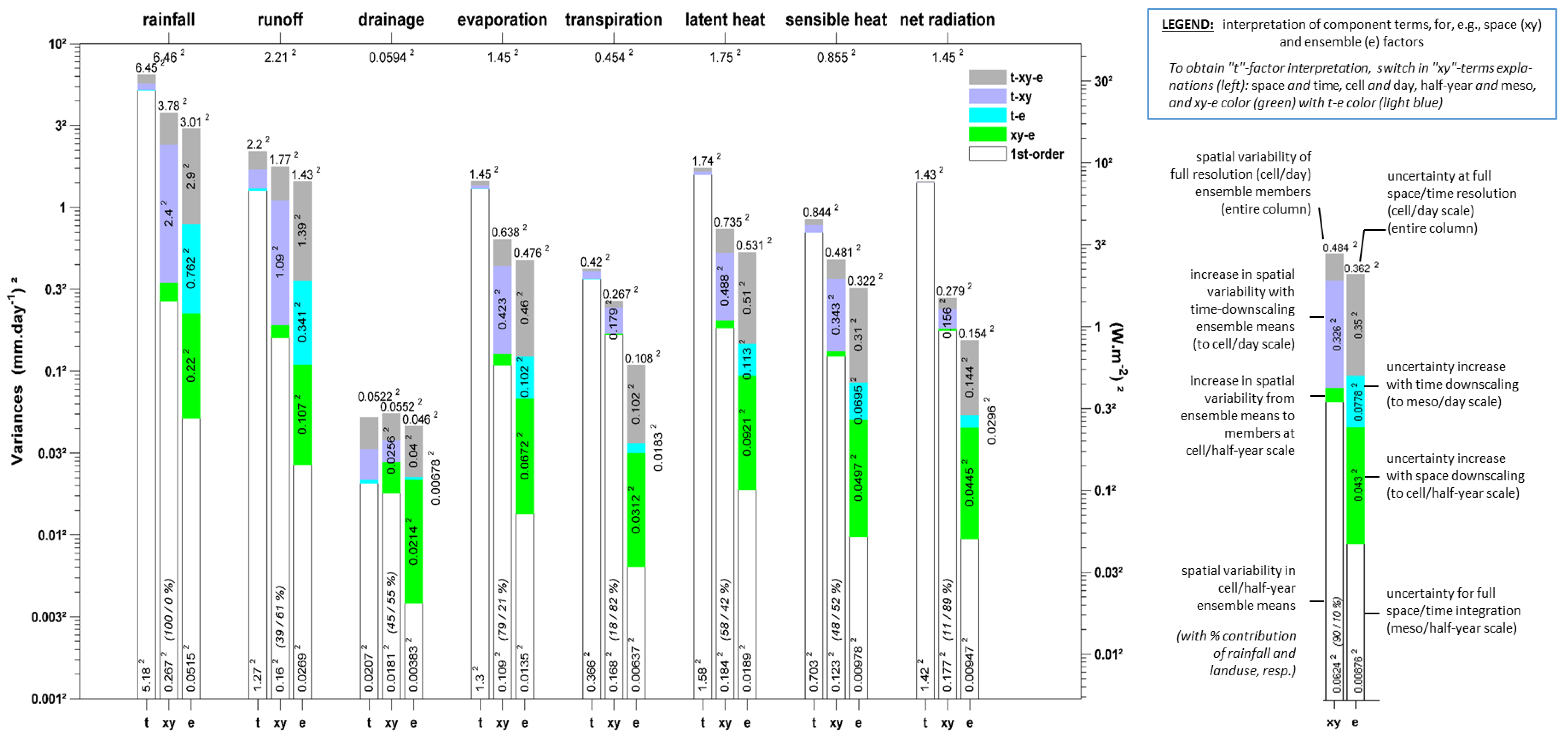
3.1.2. Global Variance Analysis of the Simulated Flux Ensemble: Confronting Variability Sources

In this section, flux variability in the entire, full-resolution, mixed-ecosystem simulated set is analyzed by decomposing total flux variance into its three orthogonal dimensions, namely time (t), space (xy), and ensemble (e). Flux variability in these different dimensions originates from corresponding variability in model forcings, namely: (i) time dependencies in rainfall, meteorology, and vegetation phenology, (ii) spatial variability in rainfall and ecosystem distribution, and (iii) rainfall uncertainty, for t, xy, and e respectively. This variance decomposition allows us to compare the respective effects of these different sources and to highlight those due to their interactions, through lumped measures over the whole time/space simulation domain. Analyzing temporal and spatial effects informs on how fluxes scale over time and space. It also highlights the time/space scaling of the third factor’s effects, namely flux uncertainty (taken here as the fully-lumped squared standard uncertainty, USD2).
Figure 5 displays this global variance decomposition for the different water and energy fluxes. Interpretation of the various component terms is detailed in the figure legend (right side). Taking, for instance, the uncertainty factor “e” for each flux type, the 1st-order uncertainty term amounts to the time/space-independent variance, i.e., uncertainty on the fully-integrated, meso/half-year flux. Adding either the «t-e» or the «xy-e» 2nd-order interaction term leads to the aggregated uncertainty on time or space-distributed fluxes, i.e., to uncertainty at meso/day or cell/half-year scales, respectively. Including both interaction terms as well as the 3rd-order «t-xy-e» (entire «e» bars in Figure 5) provides the finest, cell/day scale aggregated uncertainty. Similarly, the 1st-order term for the time or space factor represents the variance of the time-distributed (meso/day) or the space-distributed (cell/half-year) expected fluxes, respectively (decomposition of the latter into precipitation and land-use contributions is also reported in the figure). Adding these two 1st-order terms and the «t-xy» interaction produces the variance of expected fully-distributed (cell/day) fluxes. Entire time (left) or space (middle) bars represent total temporal or spatial variance in fully-resolved ensemble fluxes, aggregated over all ensemble members, and cells or days, respectively. Other combinations of terms provide further meaningful expressions of partial variances in the three-factor decomposition space (see legend).
As suggested in Section 3.1.1, the time factor (time-wise variability in forcings) dominates total variance for all variables—albeit less sharply for Dr (Figure 5). Its 1st-order component alone (time factor without interactions with space and uncertainty, i.e., ensemble- and space-averaged fluxes) even exceeds the other factors’ total variance except for Q and Dr. The relative effect of uncertainty on time variability is comparatively lower than that on space variability (see next paragraph). The space factor comes next in importance in the variance budget, but with a lesser 1st-order contribution (cell/half-year expectations), and mostly 2nd-order interaction with time (cell/day expectations) and 3rd-order interaction (full resolution ensemble). Direct interaction with uncertainty is less substantial, yielding moderate added spatial variability from expectations to ensemble at the cell/half-year scale (max. factor 2.4, for Dr). The uncertainty-induced spatial variability increase is always higher at daily scale (factor up to 8.8, for P), due to the 3rd-order term. Decomposition of spatial variability alone (1st-order term, i.e., for cell/half-year expectations) between precipitation and land-use largely varies with flux type (Figure 5). While the land-use factor dominates strongly for Tp and Rn, and to a lesser degree for Q, the two factors are rather balanced for Dr and H, and precipitation dominates only for Es and LE, not to speak of P itself. Note that this effect of land use (and hence the whole spatial variability) is largely tempered by the mixed-ecosystem composition of cells.
For the uncertainty factor, 1st-order terms (meso/half-year uncertainty) are much smaller than the interaction terms. Second-order interaction—hence downscaling—with time is stronger than with space for P, Q, and to a lesser extent Es and H, weaker for Dr, and similar for Tp and Rn. Further separating the spatial factor into its precipitation and land-use induced components, confirms (not in figure) that this interaction of space with uncertainty arises from the first component (precipitation) alone essentially, albeit also from the 3rd-order interaction with the two spatial components for Dr. Most important, however, is the 3rd-order interaction with both time and space, which dominates by far the composition of ensemble variability. These successive jumps in the magnitude of component uncertainty terms when moving from first to second and to third order induce very strong scale dependence of total uncertainty for all flux types.
Variance decomposition highlights the relationships existing between the variance components induced by the different factors. For instance, the decrease in variable uncertainty with spatial upscaling from cell/half-year to meso/half-year scales is identical to the decrease in spatial variability between ensemble members and their expectations at cell/half-year scale (see Figure 5 legend, common 2nd-order term to the uncertainty and space factors, in green). The same holds between the time and uncertainty factors (light-blue 2nd-order term), or between time and space (dark blue 2nd-order term), or still between the three for the 3rd-order term (gray). Also, considering the different types of variability simultaneously allows us to compare their respective magnitudes. For instance, it can be seen that uncertainty comes relatively close to spatial variance in the ensemble set (ratio ≥ 30%) for P, Q, Dr, and Es at cell/day or cell/half-year scale, also for daily LE, H, and Rn. It is smaller for Tp at both timescales and for the energy fluxes at a half-year scale. This ratio generally decreases with time upscaling and falls below 4% for Tp and Rn at cell/half-year scale. If comparing now with spatial variability of expected fluxes: (i) at cell/day scale, uncertainty comes out larger for P, Q, Dr, Es, and similar for LE and H; (ii) at cell/half-year scale, it is still larger for Dr and similar (ratio of 47%–72%) for P, Q, and Es.

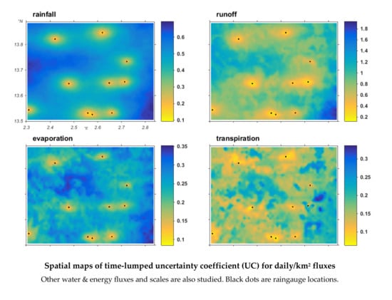
3.2. Patterns of Distributed Uncertainties

3.2.1. Distributions of Elemental Uncertainty

A first picture of the distribution of ensemble flux anomalies arising from rainfall uncertainty—the departures of ensemble members from expected fluxes—is provided by the deviations of frequency quantiles from the 1:1 line in Figure 3 and Figure 4, in relation to ensemble means, for the various flux types at cell/day and cell/half-year scales, respectively. The time-dependence of uncertainty-generated anomalies at cell/daily-scale is depicted by the deviations of frequency quantiles from means in Figure 2. Ensemble anomalies can be condensed to the elemental (unlumped) standard uncertainties USD, to characterize the distribution of uncertainties over the time/space simulation domain for the various time and space scales. Figure 6 displays the frequency distributions at full, cell/day resolution of this elemental USD, both conditioned to ensemble means and as marginal distributions over the whole domain. Figure 7 shows, for the cell/half-year scale, the direct scatter of elemental USD against means, with color intensity mapping by the rainfall uncertainty coefficient UC (Section 2.4), as well as their marginal distributions both for the ecosystem mosaic and for individual ecosystems. Table 2 gives summary statistics of elemental USD at various scales.

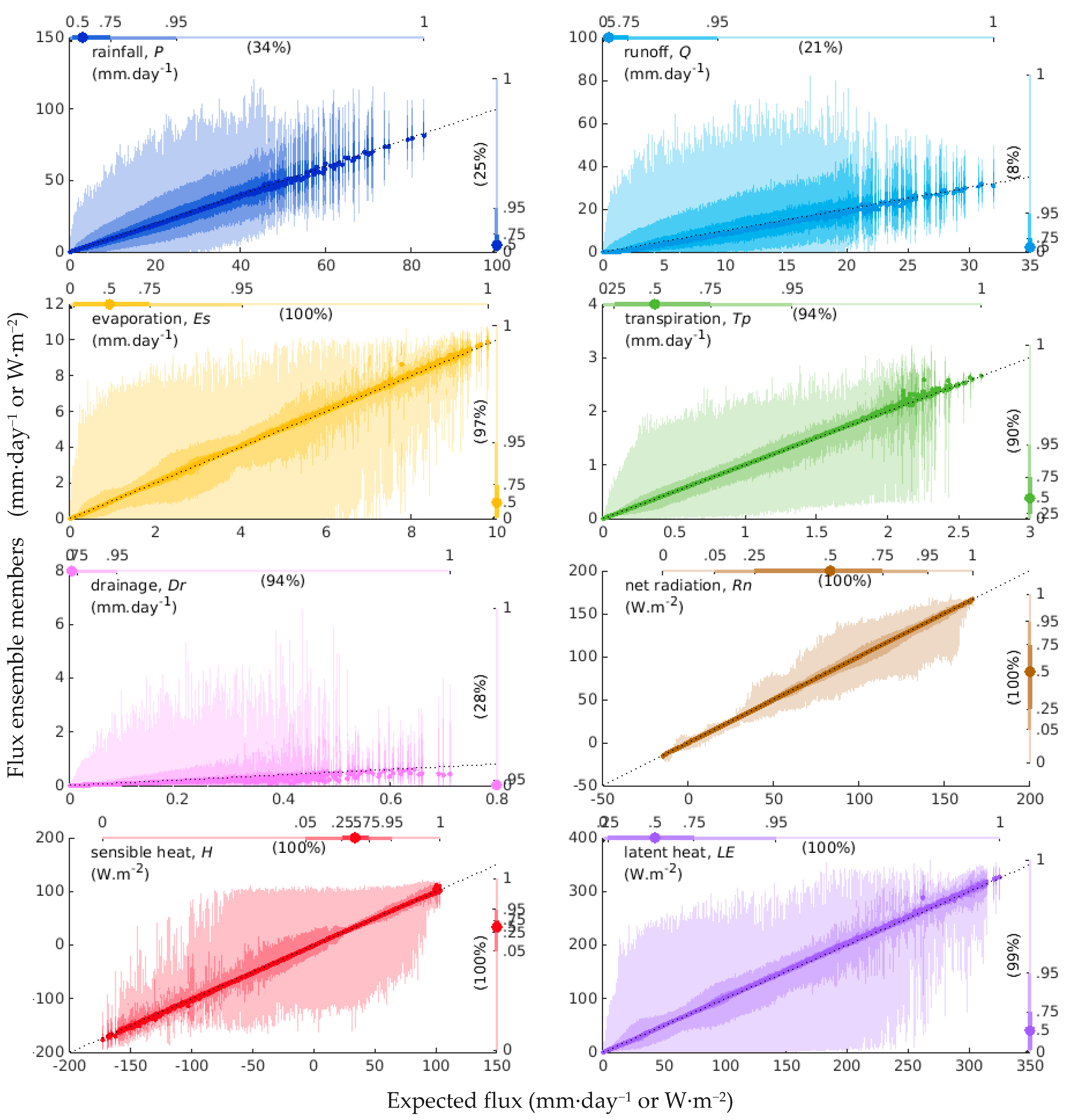
3.2.2. Relating Flux Uncertainty to Flux Magnitude

The figures displaying ensemble member variability (Figure 3 and Figure 4) or standard uncertainty (Figure 6 and Figure 7) versus expected fluxes, suggest that space/time distributions of uncertainty are strongly imprinted by those of the underlying flux magnitudes. This is also hinted at by the general relative similarity in dimensionless statistics (especially coefficient of variation and skewness, see Table 2) between the fluxes—ensemble members and means—and their uncertainties, for any given flux type and scale.
At both timescales—daily or half-year—uncertainties generally grow with flux magnitudes, more or less clearly depending on flux type. On a daily scale however (Figure 6), for most flux types, they tend to level off for large magnitudes or even to decrease for the largest ones. At least part of this originates from this effect being present in P, meaning that rainfields are likely to be better constrained by the raingauge network for the strong events than for those with lower daily intensities. This results in a saturation-type effect on extreme member values for most flux types, which limits the differences in the range between the marginal distributions of means and members (Figure 2).
A particularly strong relationship—from flux magnitude to standard uncertainty—is obtained for P, Q, and also Dr when only the time dimension is expounded (i.e., meso/day or space-lumped cell/day scales—not shown). Conversely, when the space dimension is made explicit (cell resolution, no spatial lumping), the geometrical relationship to the gauge network layout also comes into play, as it controls the degree of source uncertainty and hence blurs the relationship to flux magnitude.
Except for Rn, uncertainties in daily fluxes (Figure 3 and Figure 6) generally tend to be comparatively lower for the most frequent flux magnitudes (see, e.g., the case of H).
When intercomparing flux types, Figure 7 highlights at cell/half-year scale the stronger response to rainfall uncertainty in relative uncertainty (uncertainty coefficient UC, represented by the slope from the origin in Figure 7) for Q and especially Dr compared with Es and Tp. Uncertainties are amplified relative to P for Q and Dr but attenuated for Es and Tp. Similarly, for energy budget components, LE and H display much higher relative sensitivity to rainfall uncertainty than Rn. It is shown in Section 3.3 that, taken relative to flux magnitude (i.e., as UC) as well as to its space/time variability (i.e., as UF), uncertainty is comparatively highest for Dr and lowest for Rn at all scales. It is also shown that UC makes the most powerful dimensionless uncertainty measure, and is therefore used intensively in the following.

3.2.3. Relationship to Rainfall Uncertainty: Uncertainty Propagation Patterns

The color darkness patterns in Figure 7 provide evidence of a relationship in flux USD, and even more so in flux UC (slope from the origin), to rainfall UC, for most flux types at the cell/half-year scale. The flux uncertainty-to-expectation relationship at cell/daily scale is also well structured by the cell/half-year rainfall UC for Q and Dr but less so for the other flux types (not shown). This section further analyzes the relationship in UCs between rainfall and each dependent flux type, when projected either in the temporal or the spatial dimension. In time-wise analysis, time-distributed fluxes are considered either integrated over space (mesoscale) or at cell scale with the uncertainty measure being lumped over space. Conversely, the space-wise analysis considers both daily cell fluxes with time-lumped uncertainty and time-integrated cell fluxes.
• Time-wise analysis (temporal patterns).
Figure 8 displays the seasonal courses of space-independent UCs for 10-day fluxes taken either at cell (space-lumped UCs, Figure 8a) or meso (space-integrated fluxes, Figure 8b) spatial resolution. Despite the different space scales, note the similarity in shapes between the two graphs. The source, rainfall uncertainty follows a time pattern that is roughly opposite to that of the flux itself (Figure 2a), which is a consequence of P uncertainty scaling tightly with magnitude (Section 3.2.2) according to a concave (roughly square-root) relationship. Q closely follows the P pattern, with a relatively constant amplification factor of around 2 and 3 for cell and mesoscale fluxes (Figure 8a,b), respectively. The P pattern can be seen as propagating with more or less distortion/smoothing and lag to most of the other flux types. Only Dr appears to be less connected to the P pattern, with a much smoother course presumably due to a more time-integrative response of this flux type to rainfall. Logically, Es and LE show a high correlation, as do, less expectedly, Tp, and Rn (with uncertainty in Rn essentially coming from the upwelling thermal radiation). The abrupt hollow in the curves for several flux types after Julian day 280 is due to some light late-season rainfall with no injected uncertainty (as can be seen in Figure 2a). Note that despite the different behaviors, flux type ranking remains overall relatively time-invariant. Amplitudes of ranges in UC largely vary with flux type, e.g., for cell-scale fluxes (Figure 8a), from a factor of ~3 for P and Q to as much as ~7 for Tp.
• Space-wise analysis (spatial patterns).
Using again the UC dimensionless measure, Figure 9 displays the spatially-variable (one point per cell) relationship to rainfall uncertainty of all water and energy flux uncertainties, for daily-scale fluxes (time-lumped measure, Figure 9a) or half-year fluxes (Figure 9b). On both graphs, diagonal projection to the right or top graduated axes provides the ratio of the two confronted UC values, i.e., the corresponding UC propagation factor. For time-integrated fluxes (Figure 9b), quantile distributions of the propagation factor are also drawn on the right side of the graph (with diagonal reading), for the mixed-ecosystem cells as well as for individualized ecosystems.
It can be seen that for both timescales the relationships of flux-to-rainfall uncertainties are fairly to very strong, depending on flux type. Dr is the least strong, including a few points scattered away from the main cloud: this is likely due to this flux acting as a residual from all other water cycling processes, hence integrating all variability sources that affect the various other fluxes. Because of spatial independence in simulated flux processes (no interaction between cells, unlike over time; spatial relationships stem from forcings only), flux uncertainty in a given cell depends on the rainfall ensemble for that cell only. Figure 9 shows that this dependence is rather well summarized using the UC uncertainty measure applied to rainfall and to the various dependent fluxes.
With daily scale fluxes, even for flux types for which the relationship is very strong (e.g., Es), the corresponding propagation ratio generally varies somewhat with the level of P uncertainty, e.g., decreasing from ~0.9 to ~0.5 (i.e., increased attenuation) for Es when rainfall UC sweeps the recorded range (0.15–0.7). Only for Q is the trend slighter, and opposite (propagation ratio increasing from slightly below to slightly above 2). Relationships generally appear even stronger and propagation ratios more invariant (linear relationship) when fluxes are considered at the time-integrated scale.
Given the generally moderate variations in propagation ratios for any given individual flux type in Figure 9 (especially 9b), compared to differences between flux types, a clear hierarchy in the uncertainty measure emerges over space between flux types. This hierarchy, which varies somewhat with the timescale, is hence well summarized by the fully-lumped UC, which is mapped as big circles in Figure 9 for both timescales. These are well centered within the corresponding space-resolving clouds—except for Dr for reasons explained above. Hence the analysis of fully-lumped measures as developed in Section 3.3 can be considered to largely represent the properties of space-distributed variables as well, especially in terms of propagation effects.
Note that for both timescales, UC propagation for spatially-distributed fluxes come out nearly everywhere as amplification for Q and Dr but attenuation for all other fluxes, with only very rare exceptions for Dr at daily scale and Tp at half-year scale. This quasi-invariance also holds over time for the 10-day scale (Figure 8).
The maps in Figure 10 illustrate how the spatial patterns in time-lumped UC of daily-scale P propagate to the other flux types. The marked pothole structure of P uncertainty is largely preserved for Es and LE as well as for H, Rn, and Q and to a lesser extent for Tp, but is considerably blurred in Dr.

3.2.4. Effects of Ecosystem Type on Uncertainty

The discussion of distributed uncertainties has so far considered a cell as an integrated mix of multiple ecosystems. This subsection discusses the information characterizing the different ecosystem types for time-integrated fluxes in Figure 7 and Figure 9b.
In terms of USD (Figure 7), significantly higher values among ecosystem types are obtained for the following combinations: bare soil for Q, crops for Dr, old fallow for LE and H. All of these four combinations but the last one—old fallow with H—also correspond to the highest flux magnitudes of all ecosystem types, for the given flux type (Figure 7, top). Conversely, statistically lower USD among ecosystem types is obtained from bare soil for all energy components (Rn, H, and LE), all of which also correspond to lower flux magnitudes. This property of bare soil could also be extended to Tp and Dr, but in this case, flux magnitudes are irrelevant or insignificant for those flux types. Differences in evaporation USD between cover types are not significant, despite larger differences in flux magnitude.
In terms of the relative uncertainty UC, it can be seen in Figure 9b that distributions of UC propagation factors are lowest from bare soil for Q, Es, and Rn, from crop fields for Dr and Tp (values for these latter flux types are not quite meaningful for bare soil, see above), and from both cover types for H. Es from bare soil even displays, in statistical terms, both the lowest USDs (slightly) and the highest flux magnitudes of all ecosystem types (Figure 7). Conversely, relative sensitivity is statistically highest from the old fallow type for Dr (but with very low flux magnitude) and H, from both young and old fallow for Tp and Rn, and the crop type for Q (lowest USD but also lowest magnitude). Propagation factor distributions are hardly distinguishable between these three vegetated ecosystem types for Es, and to a lesser extent for Rn. For Q, differences between all types are much smaller in the middle of the wet spells than in the drier spells (not shown).

3.3. Scaling of Fully-Lumped Uncertainty Measures and Propagation Factors

The global variance analysis of Section 3.1.2 (more precisely, the combinations of variance component terms for the “e” factor in Figure 5) as well as the uncertainty statistics in Table 2, indicate the effects of scale on the uncertainty measures. They suggest for instance a predominance of timescale over space scale effects for some flux types. This section analyzes quantitatively these scale effects, for both standard and non-dimensional fully-lumped uncertainty measures as well as for corresponding propagation factors. For dimensionless uncertainty, both UC and the uncertainty fraction UF are considered and compared.
• Uncertainty measures.
Figure 11a–c (top three graphs) display the scale dependency for the three uncertainty measures USD, UC, and UF, respectively. Time and space scales are combined multiplicatively in a single scale measure—of dimension [T]. [L]2—along the horizontal axis, and include intermediate timescales. This combination of dimensions stems from considering the count of additive aggregation operations applied to full-resolution flux values when upscaling these fluxes.
While USDs logically decrease steadily with any upscaling for all flux types (Figure 11a), this is also true with UCs (although very mildly for time upscaling of Dr, Figure 11b), but not with UFs for which patterns of variation strongly vary depending on time and space scales (Figure 11c).
Rankings of flux types in USD are invariant with scales, namely in decreasing order: P (the source uncertainty), Q, Es, H, Rn, Tp, and Dr. These rankings change when considering dimensionless uncertainty UC and UF, however, as with USD they remain relatively stable across scales, and also between the two dimensionless measures (Figure 11b,c; high: Dr and Q; low: Rn, Es, and Tp; P intermediate). Only H moves from rather low in UC to intermediate in UF, and even high for some large timescales. This relative similarity in flux type rankings for the two dimensionless uncertainty measures UC and UF, and the much more stable, regular behavior of UC across scales that contrasts with the loss of significance of UF for the largest scales, justify that only UC was used as the dimensionless measure in Section 3.2.3. Also note that for all scales, the spread in UC across flux types is larger than that in UF.
Figure 11a,b suggests that, for any given flux type, the time scaling effect (slope of plain lines in the log space) on USD or UC is nearly independent of the space scale (two plain lines, for cell or meso), and vice-versa. If these scale effects are approximated as power relationships of (standard or dimensionless) uncertainty ratio ru to scale ratio s over the scale ranges, then combined time and space scaling can be written as:
ru ≈ (st) αt (sxy)αxy
where st and sxy denote given time and space scaling ratios, ru is the corresponding ratio for the uncertainty measure, and αt and αxy are the mean time and space scaling exponents for the considered uncertainty measure and flux variable. Table 3 displays the values of these exponents (as the mean ± the half range-width), estimated from the line vertices (full-scale ranges) in Figure 11a,b. The generally small range-widths testify to the independence suggested above.
The space scaling effect is quite invariant across the different flux types for both USD and UC (Figure 11a,b, respectively), and rather similar between these two uncertainty measures (Table 3). For USD, the time scaling effect is stronger than space scaling for the flux types with the largest USDs (P, Q, Es, LE, and H), and vice-versa for Dr. Fluxes with intermediate USD (Rn, Tp) display comparable time and space effects. Except for Dr and to a lesser extent Tp, differences between time and space scaling are smaller for UC than for USD. Note the very small time scaling effect for drainage UC.
The departure from a value of −0.5 of exponents for USD (first two columns in Table 3 and Figure 11a) reflects the degree of autocorrelation in flux anomalies over space or time (a −0.5 exponent would correspond to no autocorrelation and a null exponent to perfect correlation with homoscedasticity; see Appendix D). Thus it can be seen that ensemble anomalies in P appear fully independent over time for scales from daily upwards, due to independent simulation of rain events (Section 2.2). This is also the case to a slightly smaller degree for Q, presumably due to a slight memory effect through antecedent moisture conditions for runoff generation (see, e.g., [80]). Tp and even more so Dr anomalies are logically the most time-autocorrelated, because of the much longer response times associated with these flux types. Hence it is the system’s processes that induce time-correlation in anomalies (through correlation in fluxes), as rainfall is devoid of such correlation over the range of timescales considered. Conversely, rainfall appears to be the main source of spatial autocorrelation for the simulated system, resulting in inverse flux type rankings (the only other possible source of spatial flux correlation being land use, which appears much less effective in this respect than does rainfall).
While it could be seen in Figure 9 that Es and H have very close UCs at cell scale, Figure 11b shows that this is true at all scales, and Figure 8 that it holds over a large part of the season when the measure is resolved over time. Transpiration UC is not very different in magnitude, with a change in ranking versus the above when timescale changes, but not when space scale changes.
• Propagation factors.
The bottom graphs in Figure 11d–f display similarly, for each of the above three uncertainty measures, the scaling with time and space of the uncertainty propagation factor for each flux type, i.e., the ratio of the corresponding uncertainty measure value to that of rainfall.
When considering USD (Figure 11d), propagation factors are as expected all below unity, the highest being for Q at a nearly scale-independent value of ~0.5: USDs in Q are about half those in P. For the other flux types, USD propagation factors slightly decrease with space scale but sharply increase with the timescale, ranging 0.01–0.16 for daily fluxes versus 0.07–0.30 for half-year fluxes (lower bounds for Dr, upper bounds for Es). This reflects the generally faster USD decrease with the timescale for rainfall than for these other fluxes (see also Table 3).
With UC, Figure 11e shows that the propagation effect (either amplification or attenuation) is consistent over the whole range of time and space scales for all flux types: Dr and Q produce amplification at all scales, while all others produce attenuation. Amplification increases with scale for Dr (from a factor ~2 to ~10 over timescales) and to a lesser extent for Q (from <2 to <3). Attenuation is stable and similar for Es and H (~0.4–0.5), but decreases (rising <1 propagation factors) with time upscaling for Tp (from ~0.3 to >0.6) and Rn (in the ~0.07–0.16 range).
When comparing propagation of the two dimensionless measures UC and UF (Figure 11e,f), the same observations made in the previous sub-section for the comparison of UC and UF logically hold for their respective propagation factors. Additionally, besides the already-noted general similarity in rankings for fine scales and its decay with increasing scales due to UF scale instability (especially over time), this behavior applies when considering the nature (attenuation versus amplification) of the propagation (Figure 11f). This property further promotes UC as a better dimensionless measure of uncertainty patterns across the range of time and space scales.

4. Discussion and Conclusions

Using (i) a stochastic time/space rainfield generator, conditioned to raingauge records and reflecting the induced rainfall uncertainty, and (ii) the SEtHyS-Savannah land surface model—both calibrated against AMMA-CATCH field-data—a fine-resolution, ensemble simulation of water and energy surface fluxes was produced over a 2530-km2 domain in South-West Niger for the 2005 monsoon season and subsequent dry-down (six-month total duration).
A detailed analysis of water—including rainfall P—and energy flux variabilities in the time, space, and ensemble dimensions was performed over a wide range of time and space scales, from the day and kilometer up to the entire simulated time/space domain. Variability in the ensemble dimension reflected the propagation of P uncertainty. Sources of spatial flux variability were rainfall and land use (ecosystem types), those of temporal variability were rainfall, meteorology, and vegetation phenology. Variability was described in the form of both distributions of simulated fluxes and their first-order statistical moments (variances/standard deviations), including global variance analysis of the simulated ensemble set.
The global variance analysis allowed characterizing the respective weights of, and interactions between, the three main sources of variability, namely spatial (from cell to meso) and temporal (daily to seasonal) variability in model forcings (rainfall, meteorology, and ecosystem type) as well as rainfall uncertainty. Interaction terms were found to be especially important, making, for example, spatial variability substantially higher when accounting for full flux uncertainty than when considering ensemble means—i.e., expected fluxes—only, especially at the daily scale. The effect of ecosystem type on flux variability was found to be significant for all flux types, but not generally exceeding the rainfall uncertainty effect. Respective weights of land use versus rainfall in first-order spatial flux variability varied greatly with flux type.
Uncertainty patterns were further investigated using synthetic measures of ensemble variability, taken either at each node of the time–space domain for a given scale or lumped over one or both time–space dimensions at that scale. In addition to a dimensional measure represented by the ensemble standard deviation—denoted as standard uncertainty (USD)—two dimensionless measures were used. Denoted as uncertainty coefficient (UC) and uncertainty fraction (UF), they were obtained by normalizing USD with the quadratic mean flux or with the total standard deviation in the simulated set for that flux type, respectively.
For most flux types, space/time distributions of uncertainty were found to be highly imprinted by the distributions of flux magnitudes, with a generally positive relationship between the two variables. This relationship tended to level off for the largest magnitudes at the daily scale, starting with P.
The relationship of flux uncertainty to P uncertainty was investigated by analyzing the distributions over time or space of UC propagation patterns—from rainfall to the various flux types—using the UC measure lumped over the non-analyzed—time or space—dimension (if applicable). This analysis highlighted general invariance over space in propagation direction (amplification versus attenuation) for all flux types at any timescale, with propagation factors showing less variation within a flux type than between flux types, for whichever daily-scale or time-integrated fluxes. Hence, with the relative exception of Dr that shows some more dispersion, the spatially-distributed UC for any dependent flux type appears to scale smoothly with that of P, irrespective of other local properties (land use and rainfall magnitude). In the time dimension, rainfall uncertainty at a given time logically impacts the various fluxes over a period of time, dependent on flux type. Interpretation of UC time series generally suggests that propagation includes a strong time-lag type of effect with a lag ranging from <1 day for runoff Q to several days for Tp. Only for Dr does the P uncertainty propagate into a completely transformed signal, suggesting large diffusion over time of instant source uncertainty.
Finally, the strong general consistency in distributed uncertainty patterns over time and space for the various flux types allowed us to summarize the effects of time and space scales using the fully domain-lumped, dimensional, and dimensionless uncertainty measures. For USD as well as UC, the ranking of the flux types was more or less scale-independent, with: (i) highest values of USD for P and Q, and lowest for Rn, Tp, and Dr in decreasing order, and (ii) highest values of UC for Dr and Q, lowest for Rn. Both measures display a highly regular scaling behavior for all variables, characterized by a steady decrease with both time and space scales. The scaling in one dimension was suggested to be nearly independent of the other dimension and to closely follow a power law. Dimensionless UC also displays a high degree of scaling invariance between flux types and between the two—time and space—dimensions, with exponents in the range −0.163 to −0.204 over space and −0.172 to −0.332 over time (except for Dr). Exponent values for USD-scaling give information on the degree of time or space autocorrelation in uncertainty on the various flux types, showing a general inverse ranking of flux types for space and time, with P at one end (highest autocorrelation in space, lowest in time) and Dr at the other end (vice-versa). Expectedly, many of the above regularities in scaling patterns were preserved in the uncertainty propagation factors. For the uncertainty coefficient UC, propagation shows amplification for Q (in the ~2–3 range) and—even more so—Dr (~2–10), but attenuation for all other flux types (0.3–0.6 for Tr, Es, LE, and H, and only ~0.1 for Rn). Hence, hydrological applications of land surface modeling appear to be the most exposed to Sahelian rainfall uncertainty, but, even though to a lesser extent, agronomic, ecological, and meteorological applications are also quite sensitive through the still substantial response in the eddy fluxes (Tr, Es, LE, and H). Uncertainty in the energy budget turns out much smaller for the available energy than for its partitioning into the turbulent heat fluxes. The highly-sensitive response of the area’s Hortonian runoff to P uncertainty was previously illustrated using a rainfall–runoff model [46].
Compared to the USD and UC measures, the other dimensionless measure UF, which is directly related to the Ω coefficient of Koster et al. [77], shows a much less regular behavior, in relation to the loss of significance of this measure when scales increase towards the time/space domain size. This suggests that the newly introduced lumped uncertainty coefficient UC could be a more efficient metric across the full range of scales, making a powerful measure of relative uncertainty for the various flux types.
Compared to a more standard sensitivity analysis of rainfall error propagation, the advantage of the stochastic ensemble method used here is that it explicitly accounts for the time and space dependence structure of P uncertainty, thus allowing us to derive global uncertainty estimates and uncertainty properties at any time/space scale included in the study domain. Limitations of this study include the single year of analysis which does not permit evaluating how results may vary over years or decades, as well as the disconnection between the meteorological and rainfall forcings that may induce some inconsistencies during rain events (unusually high evaporation conditions leading in particular to very strong negative H by artefact oasis effect). However, these particular situations are seen as too rare (<1% of time–space domain) to significantly affect our conclusions on uncertainty propagation.
Although there might be some risk in extrapolating the uncertainty propagation and scaling relationships obtained here beyond the levels of rainfall uncertainty and scales encountered in this study or outside the environment explored, the plots obtained do provide a reference for these relationships in the Sahelian context. As a spatial location with respect to the raingauge network stands as a major driver of time-lumped uncertainty of P and then of most dependent fluxes (Figure 10), a relationship could be sought between UCs for these fluxes and a synthetic indicator of this relative location, such as the geometrical component in kriging variance, that would allow generalizing the mapping of UC for the various flux types.
Finally, besides the quantification of uncertainties, an additional, valuable advantage of uncertainty-reflecting ensemble simulation is that it allows for unbiased estimation of flux expectations, by ensemble averaging. Conversely, as illustrated by Vischel et al. [46], using deterministic—even though unbiased—rainfields when these are uncertain, may lead to substantial biases in simulated fluxes, that strongly affect their inferred time/space distributions. These biases arising from the simulation with the unbiased ensemble mean rainfield, as well as those produced with presumably biased alternative, deterministic rainfall interpolation methods, are being quantified, using the ensemble mean fluxes as the reference.

Supplementary Materials

The following are available online at https://www.mdpi.com/2073-4433/11/5/465/s1, Figure S1: Sample time-aggregated member rainfields from the stochastic simulation ensemble.

Author Contributions

Conceptualization, B.C. (Bernard Cappelaere), T.V., and C.O.; methodology, B.C. (Bernard Cappelaere), D.F., T.V., and J.D.; software, T.V., C.O., S.S.-P., and B.C. (Benoit Coudert); validation, D.F., J.D., and B.C. (Bernard Cappelaere); formal analysis, B.C. (Bernard Cappelaere), D.F., and J.D.; investigation, B.C. (Bernard Cappelaere), D.F., J.D., H.B.-A.I., I.M., M.O., J.-P.C., and H.B.; data curation, B.C. (Bernard Cappelaere), and D.F.; writing—original draft preparation, B.C. (Bernard Cappelaere); writing—review and editing, B.C. (Bernard Cappelaere), D.F., J.D., T.V., and C.O.; visualization, B.C. (Bernard Cappelaere) and D.F.; supervision, B.C. (Bernard Cappelaere) and J.D.; project administration, B.C. (Bernard Cappelaere) and J.D.; funding acquisition, J.D. and B.C. (Bernard Cappelaere). All authors have read and agreed to the published version of the manuscript.

Funding

During this study, D.F. was supported by a post-doctorate fellowship from IRD. Additional support by the following French projects is gratefully acknowledged: INSU-LEFE ALMIP-2, TOSCA SMOS and MISTIGRI, and ANR-Equipex CRITEX (ANR-11-EQPX-0011). Field data were collected in the framework of the AMMA-CATCH observatory (www.amma-catch.org).

Conflicts of Interest

The authors declare no conflict of interest.

Appendix A

Glossary of abbreviations, acronyms, terms, and symbols used in the paper.
αt and αxyPower-law scaling exponents over time and space (Equation (1)), for either the standard uncertainty USD or the uncertainty coefficient UC (values in Table 3, Section 3.3, interpretation in Appendix D)
ACNAMMA-CATCH-Niger
AMMAAfrican Monsoon Multidisciplinary Analyses, an international research programme
AMMA-CATCHAMMA Couplage de l’Atmosphère Tropicale et du Cycle Hydrologique, a long-term field observatory (www.amma-catch.org)
ALMIPAMMA land model intercomparison project (www.umr-cnrm.fr/amma-moana/amma_surf/almip)
DrDrainage below the root zone
EsDirect soil evaporation
fully-resolvedat cell-day resolution (i.e., coarser in time that actual model computation resolution)
half-yearthe full, 183-day study period (15 June to 14 December 2005)
HSensible heat flux
LCEcosystem/Land Cover type
LELatent heat flux
LSMLand Surface Model
meso scalethe scale of the entire, 2530-km2 study area
P, QRainfall, runoff
SEtHyS-SavannahLSM “Suivi de l’Etat Hydrique des Sols”, version dedicated to dry savannah modelling
TpPlant transpiration
SPOT-HRVHigh resolution visible images from the SPOT satellite system
UC, uncertainty coefficientThe non-dimensional uncertainty measure defined as the ratio of the standard uncertainty USD (below) to the quadratic-mean flux expectation at the same scale (see Section 2.4 and Appendix B)
UF, uncertainty fractionThe non-dimensional uncertainty measure defined as the ratio of the standard uncertainty USD (below) to the overall standard deviation of the entire multidimensional simulated ensemble set for the same flux type and scale (see Section 2.4 and Appendix B)
USD, standard uncertaintyThe dimensional uncertainty measure computed as the ensemble standard deviation for the considered flux type and scale (see Section 2.4 and Appendix B)

Appendix B

This appendix provides the mathematical expressions of the various flux operations and measures used to synthesize ensemble distributions in the simulated set, for a given flux type f taken at a given scale in xy,t.
Although measures are developed for mixed-ecosystem fluxes hereafter, elemental and time-lumped uncertainties displayed for individual ecosystem fluxes in Figure 4, Figure 7, and Figure 9 are computed with identical expressions, only with additional LC indexing.
(a) Mathematical expressions of aggregated fluxes and ensemble-derived measures: expectation, uncertainty measures, propagation factors (see notation conventions in (b))
  • Mixed-ecosytem flux of type f for ensemble member eat space/time location (xy,t) taken at a given space/time resolution:
    f (xy,t,e) = MLC (a(xy,LCf (xy,t,e,LC)),
    with a(xy,LC) the areal fraction of ecosystem LC at location xy.
    For (xy,t)-resolution upscaled from full resolution (cell,day):
    f (xy,t,e) = Mcell-to-xy; day-to-t (f (cell,day,e))
  • Flux expectation: Ef (xy,t) ~ Me (f (xy,t,e))
  • Uncertainty measures and associated propagation factors:Atmosphere 11 00465 i001
(b) Notation conventions used in (a).
  • Ufd1(d2) is the value of measure U for flux type f, taken at a given location in a subspace of dimension(s) d2, with measure-lumping over dimension(s) d1.
  • Operators Md, Qd, and SDd designate the arithmetic mean, the quadratic mean, and the standard deviation, respectively, applied over the dimension(s) {d}.
Notes: (i) flux type P is rainfall; (ii) if the scale for a dimension, xy and/or t, corresponds to the maximum degree of aggregation of fluxes f in that dimension (i.e., the domain width in that dimension) then lumping is of no effect in that dimension.

Appendix C

In this appendix, the flux distributions depicted by Figure 2, Figure 3 and Figure 4 are interpreted to highlight some patterns of first-order functioning of water and energy cycles in the study domain.
From Figure 2, it can be seen that:
-
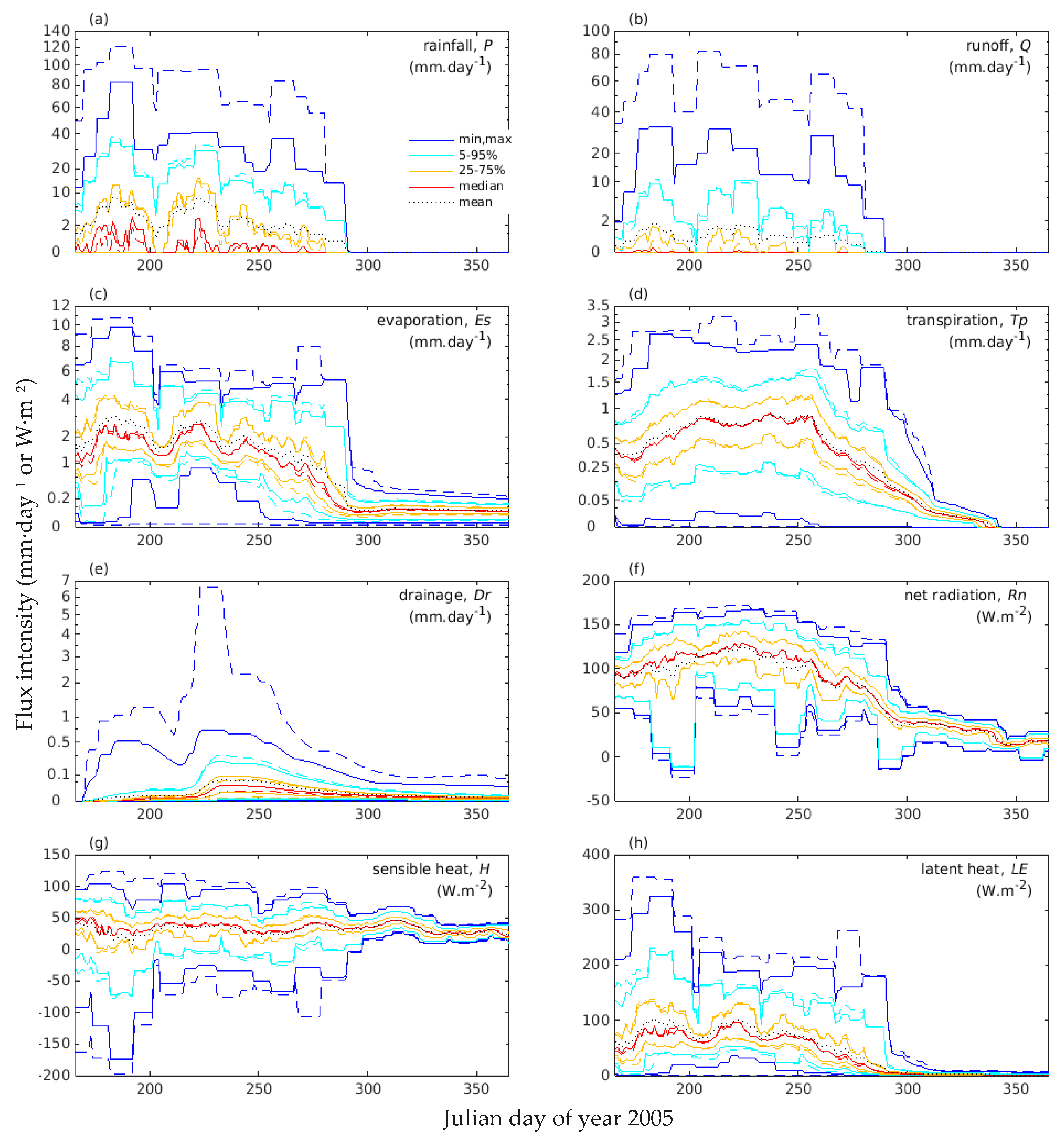
The simulation period displays the typical annual dynamics of the Sahelian climate, with a ~four-month monsoon season followed by a long, completely dry season (until the first 2006 rainfall, in May, although only represented up to mid-December).
-
Superimposed onto the general two-season annual cycle, the wet season profile is characterized by a succession of wetter and drier periods, up to a nearly monthly wavelength in rainfall. Such sub-seasonal alternations are also quite typical of the Sahelian monsoon regime.
-
This sub-seasonal P profile propagates quite directly in time to Q as well as to Es and LE, and even to Dr despite the diffusion. It also, albeit more mildly, affects the Tp signal by modulating the unimodal LAI seasonality (Figure 1b) but with some phase inversion relative to P. This inversion may be explained at least in part by the competition for energy with the direct soil evaporation process [22], with preemption of available energy by the latter in wetter periods at the expense of transpiration. Conversely, Tp is also less affected by dry spells as roots can draw on deeper water. The sub-seasonal P modulation propagates with considerable attenuation to H (and with general phase opposition relative to LE, due to energy balancing) and to Rn.
-
Figure 2, Figure 3 and Figure 4 reveal the relative weights of the various flux types in the water and energy balances at the different scales. When integrated over time (Figure 4), a clear hierarchy in flux types arises:
-
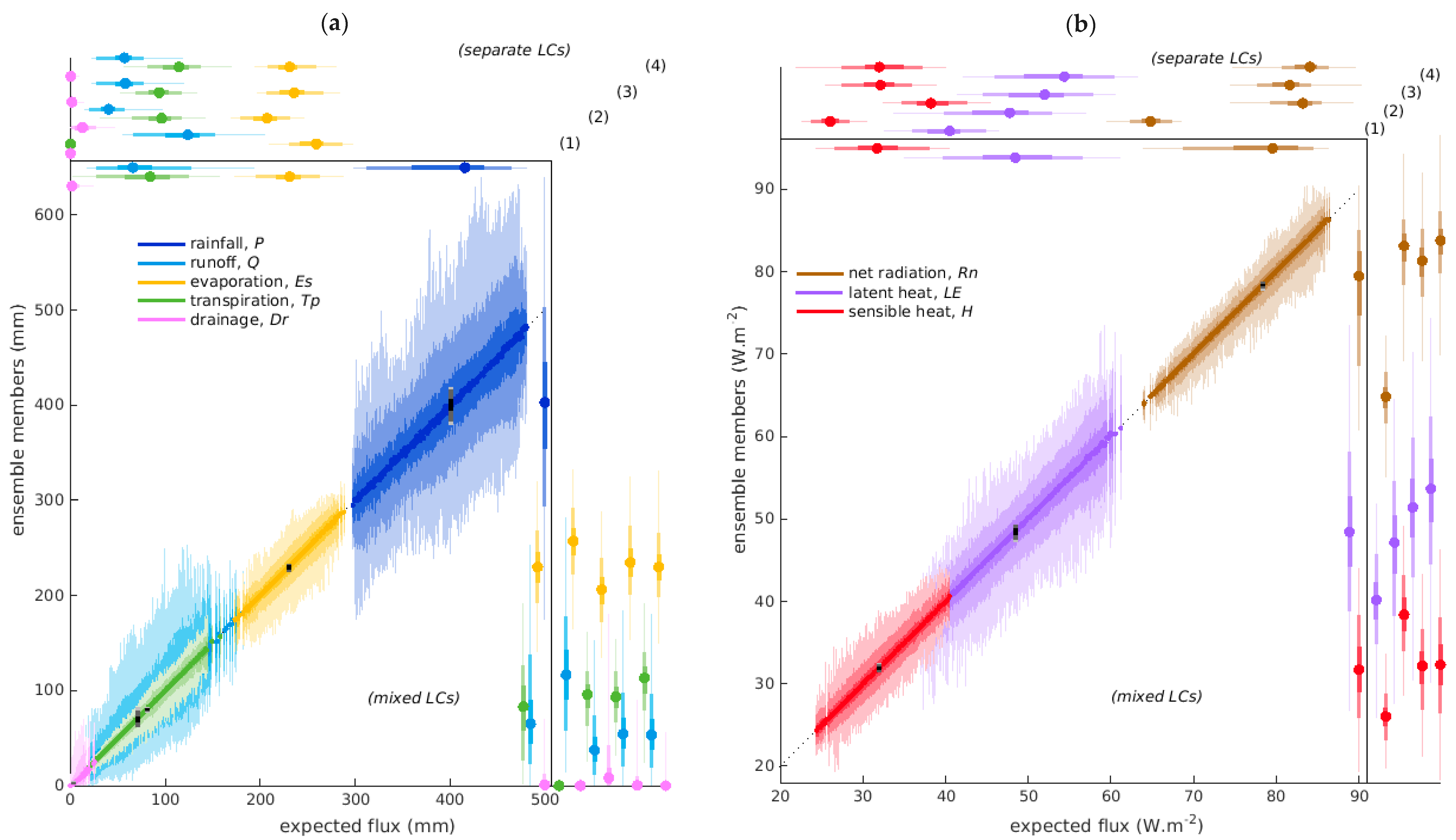
For water fluxes (Figure 4a), cell-scale ensemble members or means for Es are all greater than those for the other rainwater-redistributing fluxes at the same location, for single or mixed land covers. The range of ensemble mesoscale Es is 225–234 mm, against 379–419 mm for P, with a ratio of 57.4% for the expected fluxes. Dr is the opposite, being lowest in all cells, with an expectation of 7.3‰ of P at mesoscale and an ensemble range of 1.9–5.0 mm (note however that Dr recedes only slowly after the study period into the dry season, meaning that the ratio would be somewhat higher over a full year period). Q and Tp have intermediate magnitudes, the latter being generally the higher except in bare soil cells; mesoscale expectations are 17.6% and 20.1% of P, with ranges of 62–83 mm and 77–83 mm, respectively. Es being substantially higher than Tp agrees with the climatological analysis by Velluet et al. [22] for this area. This overall hierarchy holds throughout the period for expected fluxes at the 11-day/mesoscale (dotted running-mean curve in Figure 2), with only Tp and Q alternating in ranking: the latter predominates during the more pronounced, first two wet spells, while the opposite occurs for the weaker last two wet spells.
-
Among energy fluxes at the cell/half-year scale (Figure 4b), LE is nearly everywhere higher than H, although the reverse occurs mainly—but still infrequently—for the cropland cover. Corresponding mesoscale expectations are 62% and 41% of Rn (=78.4 W·m−2), respectively.
-
Relative weights of overall mean water and energy balance components are remarkably similar to those obtained by Velluet et al. [22], despite the differences in domain extent (space and time), data and tools, etc.
The effect of ecosystem type on the water and energy fluxes distributions is significant (distributions differ from one another and the mixed-ecosystem situation) for all flux types. However, these differences do not generally exceed the rainfall uncertainty effect (ensemble spread), except for specific ecosystem and flux type combinations (Figure 4). This is the case in particular with: (i) the bare soil ecosystem, for Rn and of course Tp, as well as to a slightly lesser degree for Q, and H and LE; (ii) the crops ecosystem, for Q, Dr, Rn, and H; and (iii) Tp from old fallow. Dr flux is significant under crops, but is barely so for young and especially old fallow, and is nil for bare soil. Overall, young fallow is the ecosystem that best represents the integrated mosaic of all ecosystems. For most flux types, bare/degraded soil and crops are the land-cover types producing the opposite extreme fluxes. These are, in means: highest Q and Es, and lowest LE, H, Rn, Dr and of course Tp for bare soil, and vice-versa for crops (note however that Tp and LE are still higher for old fallow than for the crop). Relative effects of land use and of spatial variability in rainfall on variances of expected time-integrated fluxes are described in the following section and figure.

Appendix D

Interpretation of time and space scaling exponents αt and αxy (Equation (1)) for standard uncertainty USD.
When a flux variable f is aggregated with a scale ratio s (the number of aggregated locations, either cells or timesteps) in the time or space dimension:
fs,k = [∑ik=1,s fo,ik]/s
with fs,k the upscaled flux at location k for that upper scale s, fo,ik the unscaled flux at initial-scale location ik within s-scale location k, and ∑ik the sum over locations ik.
Then the ensemble variance of the upscaled variable writes:
Var(fs,k) = [∑ikVar(fo,ik) + 2∑ik≠jkCov(fo,ik, fo,jk)]/s2
with Var(fo,ik) and Cov(fo,ik, fo,jk) the ensemble variance of fo,ik and covariance of fo,ik and fo,jk, respectively.
Denoting ns the number of locations k at scale s, the standard uncertainty USD at scale s is:
USDs = Var(fs)1/2 = {∑k Var(fs,k)/ns}1/2
Given that the standard uncertainty at initial scale o can be written as:
USDo = Var(fo)1/2 = {∑i Var(fo,i)/no}1/2 = {∑kik Var(fo,ik)/no}1/2
with no the total number of locations i at scale o (no = ns·s), then the USD scaling ratio ru = USDs/USDo simplifies to:
ru = {[1 + 2/no·∑kik≠jk Cov(fo,ik, fo,jk)/Var(fo)]/s}1/2
Introducing cross-correlation coefficients R(fo,ik, fo,jk), ru becomes:
ru = {[1 + 2/no·∑kik≠jk R(fo,ik, fo,jk) SD(fo,ik) SD(fo,jk)/Var(fo) ]/s}1/2
with SD(fo,ik) the standard deviation of fo,ik.
If fo displays no autocorrelation (R(fo,ik, fo,jk) = 0, for any ik ≠ jk), then ru = s−1/2, hence α = −0.5.
If fo displays perfect autocorrelation (R(fo,ik, fo,jk) = 1, for any ik,jk) with homoscedasticity (uniform variance), then
ru = {[1 + 2/no·ns·s(s−1)/2]/s}1/2 = 1 = s0, hence α = 0.
In the general case (partially autocorrelated and/or heteroscedastic f0), R values are between ~0 and 1, hence Equation (A1) identifies with Equation (1) (ru = sα with α increasing between ~−0.5 and 0 with R, i.e., with the degree of autocorrelation in the unscaled variable f0.
Only in the physically unrealistic case of significant anti-correlation in f (substantially negative R values), could the exponent α fall significantly below the −0.5 threshold.

References

  1. Niang, I.; Ruppel, O.C.; Abdrabo, M.A.; Essel, A.; Lennard, C.; Padgham, J.; Urquhart, P. Africa. In Climate Change 2014: Impacts, Adaptation, and Vulnerability. Part B: Regional Aspects. Contribution of Working Group 2 to the 5th Assessment Report of the I.P.C.C.; Barros, V.R., Field, C.B., Dokken, D.J., Mastrandrea, M.D., Mach, K.J., Bilir, T.E., Chatterjee, M., Ebi, K.L., Estrada, Y.O., Genova, R.C., et al., Eds.; Cambridge University Press: Cambridge, UK; New York, NY, USA, 2014; pp. 1199–1265. [Google Scholar]
  2. De Souza, K.; Kituyi, E.; Harvey, B.; Leone, M.; Murali, K.S.; Ford, J.D. Vulnerability to climate change in three hot spots in Africa and Asia: Key issues for policy-relevant adaptation and resilience-building research. Reg. Environ. Chang. 2015, 15, 747–753. [Google Scholar] [CrossRef] [Green Version]
  3. Kilroy, G. A review of the biophysical impacts of climate change in three hotspot regions in Africa and Asia. Reg. Environ. Chang. 2015, 15, 771–782. [Google Scholar] [CrossRef] [Green Version]
  4. Lebel, T.; Cappelaere, B.; Galle, S.; Hanan, N.; Kergoat, L.; Levis, S.; Vieux, B.; Descroix, L.; Gosset, M.; Mougin, E.; et al. AMMA-CATCH studies in the Sahelian region of West-Africa: An overview. J. Hydrol. 2009, 375, 3–13. [Google Scholar] [CrossRef] [Green Version]
  5. Boone, A.; de Rosnay, P.; Balsamo, G.; Beljaars, A.; Chopin, F.; Decharme, B.; Delire, C.; Ducharne, A.; Gascoin, S.; Grippa, M.; et al. The AMMA Land Surface Model Intercomparison Project (ALMIP). Bull. Am. Meteorol. Soc. 2009, 90, 1865–1880. [Google Scholar] [CrossRef]
  6. Cappelaere, B.; Descroix, L.; Lebel, T.; Boulain, N.; Ramier, D.; Laurent, J.P.; Favreau, G.; Boubkraoui, S.; Boucher, M.; Bouzou Moussa, I.; et al. The AMMA-CATCH experiment in the cultivated Sahelian area of south-west Niger—Investigating water cycle response to a fluctuating climate and changing environment. J. Hydrol. 2009, 375, 34–51. [Google Scholar] [CrossRef]
  7. Leauthaud, C.; Cappelaere, B.; Demarty, J.; Guichard, F.; Velluet, C.; Kergoat, L.; Vischel, T.; Grippa, M.; Mouhaimouni, M.; Bouzou Moussa, I.; et al. A 60-year reconstructed high-resolution local meteorological data set in Central Sahel (1950-2009): Evaluation, analysis and application to land surface modelling. Int. J. Climatol. 2017, 37, 2699–2718. [Google Scholar] [CrossRef] [Green Version]
  8. D’Amato, N.; Lebel, T. On the characteristics of the rainfall events in the Sahel with a view to the analysis of climatic variability. Int. J. Climatol. 1998, 18, 955–974. [Google Scholar] [CrossRef]
  9. Koster, R.D.; Dirmeyer, P.A.; Guo, Z.; Bonan, G.; Chan, E.; Cox, P.; Gordon, C.T.; Kanae, S.; Kowalczyk, E.; Lawrence, D.; et al. Regions of strong coupling between soil moisture and precipitation. Science 2004, 305, 1138–1140. [Google Scholar] [CrossRef] [Green Version]
  10. Petrova, I.; Miralles, D.; van Heerwaarden, C.; Wouters, H. Relation between convective rainfall properties and antecedent soil moisture heterogeneity conditions in North Africa. Remote Sens. 2018, 10, 969. [Google Scholar] [CrossRef] [Green Version]
  11. Wolters, D.; van Heerwaarden, C.C.; de Arellano, J.V.G.; Cappelaere, B.; Ramier, D. Effects of soil moisture gradients on the path and the intensity of a West African squall line. Q. J. R. Meteorol. Soc. 2010, 136, 2162–2175. [Google Scholar] [CrossRef]
  12. Hartley, A.J.; Parker, D.J.; Garcia-Carreras, L.; Webster, S. Simulation of vegetation feedbacks on local and regional scale precipitation in West Africa. Agric. For. Meteorol. 2016, 222, 59–70. [Google Scholar] [CrossRef] [Green Version]
  13. Sy, S.; De Noblet-Ducoudré, N.; Quesada, B.; Sy, I.; Dieye, A.M.; Gaye, A.T.; Sultan, B. Land-Surface Characteristics and Climate in West Africa: Models’ Biases and Impacts of Historical Anthropogenically-Induced Deforestation. Sustainability 2017, 9, 1917. [Google Scholar] [CrossRef] [Green Version]
  14. Xue, Y. Impact of Land–Atmosphere Interactions on Sahel Climate; Oxford University Press: Oxford, UK, 2017. [Google Scholar] [CrossRef] [Green Version]
  15. Van Der Wijngaart, R.; Helming, J.; Jacobs, C.; Hoek, S.; Garzon Delvaux, P.A.; Gomez y Paloma, S. Irrigation and Irrigated Agriculture Potential in the Sahel: The Case of the Niger River Basin: Prospective Review of the Potential and Constraints in a Changing Climate; Joint Research Centre (JRC): Ispra, Italy, 2019. [Google Scholar] [CrossRef]
  16. Redelsperger, J.L.; Thorncroft, C.D.; Diedhiou, A.; Lebel, T.; Parker, D.J.; Polcher, J. African monsoon multidisciplinary analysis—An international research project and field campaign. Bull. Am. Meteorol. Soc. 2006, 87, 1739–1746. [Google Scholar] [CrossRef] [Green Version]
  17. Ait Hssaine, B.; Ezzahar, J.; Jarlan, L.; Merlin, O.; Khabba, S.; Brut, A.; Er-Raki, S.; Elfarkh, J.; Cappelaere, B.; Chehbouni, G. Combining a two source energy balance model driven by MODIS and MSG-SEVIRI products with an aggregation approach to estimate turbulent fluxes over sparse and heterogeneous vegetation in Sahel region (Niger). Remote Sens. 2018, 10, 974. [Google Scholar] [CrossRef] [Green Version]
  18. Braud, I. Spatial variability of surface properties and estimation of surface fluxes of a savannah. Agric. For. Meteorol. 1998, 89, 15–44. [Google Scholar] [CrossRef]
  19. Hanan, N.P. Enhanced two-layer radiative transfer scheme for a land surface model with a discontinuous upper canopy. Agric. For. Meteorol. 2001, 109, 265–281. [Google Scholar] [CrossRef]
  20. Marshall, M.; Tu, K.; Funk, C.; Michaelsen, J.; Williams, P.; Williams, C.; Ardö, J.; Boucher, M.; Cappelaere, B.; Grandcourt, A.; et al. Improving operational land surface model canopy evapotranspiration in Africa using a direct remote sensing approach. Hydrol. Earth Syst. Sci. 2013, 17, 1079–1091. [Google Scholar] [CrossRef] [Green Version]
  21. Ridler, M.E.; Sandholt, I.; Butts, M.; Lerer, S.; Mougin, E.; Timouk, F.; Kergoat, L.; Madsen, H. Calibrating a soil-vegetation-atmosphere transfer model with remote sensing estimates of surface temperature and soil surface moisture in a semi arid environment. J. Hydrol. 2012, 436, 1–12. [Google Scholar] [CrossRef]
  22. Velluet, C.; Demarty, J.; Cappelaere, B.; Braud, I.; Issoufou, H.B.A.; Boulain, N.; Ramier, D.; Mainassara, I.; Charvet, G.; Boucher, M.; et al. Building a field- and model-based climatology of local water and energy cycles in the cultivated Sahel—Annual budgets and seasonality. Hydrol. Earth Syst. Sci. 2014, 18, 5001–5024. [Google Scholar] [CrossRef] [Green Version]
  23. Verhoef, A.; Allen, S.J. A SVAT scheme describing energy and CO2 fluxes for multi-component vegetation: Calibration and test for a Sahelian savannah. Ecol. Model. 2000, 127, 245–267. [Google Scholar] [CrossRef]
  24. Getirana, A.; Boone, A.; Peugeot, C.; ALMIP-2 Working Group. Streamflows over a West African basin from the ALMIP-2 model ensemble. J. Hydrometeorol. 2017, 18, 1831–1845. [Google Scholar] [CrossRef]
  25. Grippa, M.; Kergoat, L.; Boone, A.; Peugeot, C.; Demarty, J.; Cappelaere, B.; Gal, L.; Hiernaux, P.; Mougin, E.; Ducharne, A.; et al. Modeling surface runoff and water fluxes over contrasted soils in the pastoral Sahel: Evaluation of the ALMIP2 land surface models over the Gourma region in Mali. J. Hydrometeorol. 2017, 18, 1847–1866. [Google Scholar] [CrossRef]
  26. Saux-Picart, S.; Ottlé, C.; Perrier, A.; Decharme, B.; Coudert, B.; Zribi, M.; Boulain, N.; Cappelaere, B.; Ramier, D. SEtHyS_Savannah: A multiple source land surface model applied to Sahelian landscapes. Agric. For. Meteorol. 2009, 149, 1421–1432. [Google Scholar] [CrossRef]
  27. Saux-Picart, S.; Ottlé, C.; Decharme, B.; Andre, C.; Zribi, M.; Perrier, A.; Coudert, B.; Boulain, N.; Cappelaere, B.; Descroix, L.; et al. Water and energy budgets simulation over the AMMA-Niger super-site spatially constrained with remote sensing data. J. Hydrol. 2009, 375, 287–295. [Google Scholar] [CrossRef]
  28. Bahat, Y.; Grodek, T.; Lekach, J.; Morin, E. Rainfall-runoff modeling in a small hyper-arid catchment. J. Hydrol. 2009, 373, 204–217. [Google Scholar] [CrossRef]
  29. Ogden, F.L.; Sharif, H.O.; Senarath, S.U.S.; Smith, J.A.; Baeck, M.L.; Richardson, J.R. Hydrologic analysis of the Fort Collins, Colorado, flash flood of 1997. J. Hydrol. 2000, 228, 82–100. [Google Scholar] [CrossRef]
  30. Arnaud, P.; Bouvier, C.; Cisneros, L.; Dominguez, R. Influence of rainfall spatial variability on flood prediction. J. Hydrol. 2002, 260, 216–230. [Google Scholar] [CrossRef]
  31. Messager, C.; Gallee, H.; Brasseur, O.; Cappelaere, B.; Peugeot, C.; Seguis, L.; Vauclin, M.; Ramel, R.; Grasseau, G.; Leger, L.; et al. Influence of observed and RCM-simulated precipitation on the water discharge over the Sirba basin, Burkina Faso/Niger. Clim. Dyn. 2006, 27, 199–214. [Google Scholar] [CrossRef]
  32. Segond, M.L.; Wheater, H.S.; Onof, C. The significance of spatial rainfall representation for flood runoff estimation: A numerical evaluation based on the Lee catchment, UK. J. Hydrol. 2007, 347, 116–131. [Google Scholar] [CrossRef]
  33. Vischel, T.; Lebel, T. Assessing the water balance in the Sahel: Impact of small scale rainfall variability on runoff. Part 2: Idealized modeling of runoff sensitivity. J. Hydrol. 2007, 333, 340–355. [Google Scholar] [CrossRef]
  34. Zhang, A.; Shi, H.Y.; Li, T.J.; Fu, X.D. Analysis of the Influence of Rainfall Spatial Uncertainty on Hydrological Simulations Using the Bootstrap Method. Atmosphere 2018, 9, 71. [Google Scholar] [CrossRef] [Green Version]
  35. Maggioni, V.; Reichle, R.H.; Anagnostou, E.N. The Effect of Satellite Rainfall Error Modeling on Soil Moisture Prediction Uncertainty. J. Hydrometeorol. 2011, 12, 413–428. [Google Scholar] [CrossRef]
  36. Serpetzoglou, E.; Anagnostou, E.N.; Papadopoulos, A.; Nikolopoulos, E.I.; Maggioni, V. Error Propagation of Remote Sensing Rainfall Estimates in Soil Moisture Prediction from a Land Surface Model. J. Hydrometeorol. 2010, 11, 705–720. [Google Scholar] [CrossRef]
  37. Bormann, H. Sensitivity of a soil-vegetation-atmosphere-transfer scheme to input data resolution and data classification. J. Hydrol. 2008, 351, 154–169. [Google Scholar] [CrossRef]
  38. Bitew, M.M.; Gebremichael, M. Evaluation of satellite rainfall products through hydrologic simulation in a fully distributed hydrologic model. Water Resour. Res. 2011, 47, W06526. [Google Scholar] [CrossRef]
  39. Fekete, B.M.; Vörösmarty, C.J.; Roads, J.O.; Willmott, C.J. Uncertainties in precipitation and their impacts on runoff estimates. J. Clim. 2004, 17, 294–304. [Google Scholar] [CrossRef]
  40. Stisen, S.; Sandholt, I. Evaluation of remote-sensing-based rainfall products through predictive capability in hydrological runoff modelling. Hydrol. Process. 2010, 24, 879–891. [Google Scholar] [CrossRef]
  41. Pierre, C.; Bergametti, G.; Marticorena, B.; Mougin, E.; Lebel, T.; Ali, A. Pluriannual comparisons of satellite-based rainfall products over the Sahelian belt for seasonal vegetation modeling. J. Geophys. Res.-Atmos. 2011, 116. [Google Scholar] [CrossRef] [Green Version]
  42. Nijssen, B.; Lettenmaier, D.P. Effect of precipitation sampling error on simulated hydrological fluxes and states: Anticipating the Global Precipitation Measurement satellites. J. Geophys. Res.-Atmos. 2004, 109. [Google Scholar] [CrossRef]
  43. Nikolopoulos, E.I.; Anagnostou, E.N.; Hossain, F.; Gebremichael, M.; Borga, M. Understanding the Scale Relationships of Uncertainty Propagation of Satellite Rainfall through a Distributed Hydrologic Model. J. Hydrometeorol. 2010, 11, 520–532. [Google Scholar] [CrossRef]
  44. Vieux, B.E.; Imgarten, J.M. On the scale-dependent propagation of hydrologic uncertainty using high-resolution X-band radar rainfall estimates. Atmos. Res. 2012, 103, 96–105. [Google Scholar] [CrossRef]
  45. Villarini, G.; Krajewski, W.F.; Ntelekos, A.A.; Georgakakos, K.P.; Smith, J.A. Towards probabilistic forecasting of flash floods The combined effects of uncertainty in radar-rainfall and flash flood guidance. J. Hydrol. 2010, 394, 275–284. [Google Scholar] [CrossRef]
  46. Vischel, T.; Lebel, T.; Massuel, S.; Cappelaere, B. Conditional simulation schemes of rain fields and their application to rainfall-runoff modeling studies in the Sahel. J. Hydrol. 2009, 375, 273–286. [Google Scholar] [CrossRef]
  47. Galle, S.; Grippa, M.; Peugeot, C.; Bouzou Moussa, I.; Cappelaere, B.; Demarty, J.; Mougin, E.; Panthou, G.; Adjomayi, P.; Agbossou, E.K.; et al. AMMA-CATCH—A critical zone observatory in West Africa monitoring a region in transition. Vadose Zone J. 2018, 17, 180062. [Google Scholar] [CrossRef] [Green Version]
  48. Boulain, N.; Cappelaere, B.; Ramier, D.; Issoufou, H.B.A.; Halilou, O.; Seghieri, J.; Guillemin, F.; Oi, M.; Gignoux, J.; Timouk, F. Towards an understanding of coupled physical and biological processes in the cultivated Sahel—2. Vegetation and carbon dynamics. J. Hydrol. 2009, 375, 190–203. [Google Scholar] [CrossRef]
  49. Ezzahar, J.; Chehbouni, A.; Hoedjes, J.; Ramier, D.; Boulain, N.; Boubkraoui, S.; Cappelaere, B.; Descroix, L.; Mougenot, B.; Timouk, F. Combining scintillometer measurements and an aggregation scheme to estimate area-averaged latent heat flux during the AMMA experiment. J. Hydrol. 2009, 375, 217–226. [Google Scholar] [CrossRef] [Green Version]
  50. Ibrahim, M.; Favreau, G.; Scanlon, B.R.; Seidel, J.L.; Le Coz, M.; Demarty, J.; Cappelaere, B. Long-term increase in diffuse groundwater recharge following expansion of rainfed cultivation in the Sahel, West Africa. Hydrogeol. J. 2014, 22, 1293–1305. [Google Scholar] [CrossRef]
  51. Lohou, F.; Kergoat, L.; Guichard, F.; Boone, A.; Cappelaere, B.; Cohard, J.M.; Demarty, J.; Galle, S.; Grippa, M.; Peugeot, C.; et al. Surface response to rain events throughout the West African monsoon. Atmos. Chem. Phys. 2014, 14, 3883–3898. [Google Scholar] [CrossRef] [Green Version]
  52. Pfeffer, J.; Champollion, C.; Favreau, G.; Cappelaere, B.; Hinderer, J.; Boucher, M.; Nazoumou, Y.; Oï, M.; Mouyen, M.; Henri, C.; et al. Evaluating surface and subsurface water storage variations at small time and space scales from relative gravity measurements in semi-arid Niger. Water Resour. Res. 2013, 49, 3276–3291. [Google Scholar] [CrossRef]
  53. Ramier, D.; Boulain, N.; Cappelaere, B.; Timouk, F.; Rabanit, M.; Lloyd, C.R.; Boubkraoui, S.; Metayer, F.; Descroix, L.; Wawrzyniak, V. Towards an understanding of coupled physical and biological processes in the cultivated Sahel—1. Energy and water. J. Hydrol. 2009, 375, 204–216. [Google Scholar] [CrossRef]
  54. Boone, A.; Getirana, A.; Demarty, J.; Cappelaere, B.; Galle, S.; Grippa, M.; Lebel, T.; Mougin, E.; Peugeot, C.; Vischel, T. The AMMA Land Surface Model Intercomparison Project Phase 2 (ALMIP-2). Gewex News 2009, 19, 9–10. [Google Scholar]
  55. Boulain, N.; Cappelaere, B.; Seguis, L.; Favreau, G.; Gignoux, J. Water balance and vegetation change in the Sahel: A case study at the watershed scale with an eco-hydrological model. J. Arid Environ. 2009, 73, 1125–1135. [Google Scholar] [CrossRef]
  56. Boulain, N.; Cappelaere, B.; Seguis, L.; Gignoux, J.; Peugeot, C. Hydrologic and land use impacts on vegetation growth and NPP at the watershed scale in a semi-arid environment. Reg. Environ. Chang. 2006, 6, 147–156. [Google Scholar] [CrossRef]
  57. Leauthaud, C.; Demarty, J.; Cappelaere, B.; Grippa, M.; Kergoat, L.; Velluet, C.; Guichard, F.; Mougin, E.; Chelbi, S.; Sultan, B. Revisiting historical climatic signals to better explore the future: Prospects of water cycle changes in Central Sahel. Proc. IAHS 2015, 371, 195–201. [Google Scholar] [CrossRef] [Green Version]
  58. Pellarin, T.; Laurent, J.P.; Cappelaere, B.; Decharme, B.; Descroix, L.; Ramier, D. Hydrological modelling and associated microwave emission of a semi-arid region in South-western Niger. J. Hydrol. 2009, 375, 262–272. [Google Scholar] [CrossRef]
  59. Massuel, S.; Cappelaere, B.; Favreau, G.; Leduc, C.; Lebel, T.; Vischel, T. Integrated surface water-groundwater modelling in the context of increasing water reserves of a Sahelian aquifer. Hydrol. Sci. J. 2011, 56, 1242–1264. [Google Scholar] [CrossRef]
  60. Abdi, A.M.; Boke-Olén, N.; Tenenbaum, D.E.; Tagesson, T.; Cappelaere, B.; Ardö, J. Evaluating water controls on vegetation growth in the semi-arid Sahel using field and Earth observation data. Remote Sens. 2017, 9, 294. [Google Scholar] [CrossRef] [Green Version]
  61. Allies, A.; Demarty, J.; Olioso, A.; Bouzou Moussa, I.; Issoufou, H.B.-A.; Velluet, C.; Bahir, M.; Mainassara, I.; Oï, M.; Chazarin, J.P.; et al. Evapotranspiration estimation in the Sahel using a new ensemble-contextual method. Remote Sens. 2020, 12, 380. [Google Scholar] [CrossRef] [Green Version]
  62. Tagesson, T.; Ardo, J.; Cappelaere, B.; Kergoat, L.; Abdi, A.; Horion, S.; Fensholt, R. Modelling spatial and temporal dynamics of GPP in the Sahel from earth-observation-based photosynthetic capacity and quantum efficiency. Biogeosciences 2017, 14, 1333–1348. [Google Scholar] [CrossRef] [Green Version]
  63. Tanguy, M.; Baille, A.; González-Real, M.M.; Lloyd, C.; Cappelaere, B.; Kergoat, L.; Cohard, J.M. A new parameterisation scheme of ground heat flux for land surface flux retrieval from remote sensing information. J. Hydrol. 2012, 454–455, 113–122. [Google Scholar] [CrossRef] [Green Version]
  64. Verhoef, A.; Ottlé, C.; Cappelaere, B.; Murray, T.; Saux Picart, S.; Zribi, A.; Maignan, F.; Boulain, N.; Demarty, J.; Ramier, D. Spatio-temporal surface soil heat flux estimates from satellite data; results for the AMMA experiment, Fakara supersite. Agric. For. Meteorol. 2012, 154–155, 55–66. [Google Scholar] [CrossRef] [Green Version]
  65. Sultan, B.; Janicot, S. The West African Monsoon Dynamics. Part II: The “Preonset” and “Onset” of the Summer Monsoon. J. Clim. 2003, 16, 3407–3427. [Google Scholar] [CrossRef]
  66. Lebel, T.; Parker, D.J.; Flamant, C.; Holler, H.; Polcher, J.; Redelsperger, J.L.; Thorncroft, C.; Bock, O.; Bourles, B.; Galle, S.; et al. The AMMA field campaigns: Accomplishments and lessons learned. Atmos. Sci. Lett. 2011, 12, 123–128. [Google Scholar] [CrossRef]
  67. Balme, M.; Vischel, T.; Lebel, T.; Peugeot, C.; Galle, S. Assessing the water balance in the Sahel: Impact of small scale rainfall variability on runoff—Part 1: Rainfall variability analysis. J. Hydrol. 2006, 331, 336–348. [Google Scholar] [CrossRef]
  68. Guillot, G.; Lebel, T. Approximation of Sahelian rainfall fields with meta-Gaussian random functions—Part 2: Parameter estimation and comparison to data. Stoch. Environ. Res. Risk Assess. 1999, 13, 113–130. [Google Scholar] [CrossRef]
  69. Vischel, T.; Quantin, G.; Lebel, T.; Viarre, J.; Gosset, M.; Cazenave, F.; Panthou, G. Generation of High-Resolution Rain Fields in West Africa: Evaluation of Dynamic Interpolation Methods. J. Hydrometeorol. 2011, 12, 1465–1482. [Google Scholar] [CrossRef]
  70. Fraga, I.; Cea, L.; Puertas, J. Effect of rainfall uncertainty on the performance of physically based rainfall-runoff models. Hydrol. Process. 2019, 33, 160–173. [Google Scholar] [CrossRef] [Green Version]
  71. Deardorff, J.W. Efficient prediction of ground surface-temperature and moisture, with inclusion of a layer of vegetation. J. Geophys. Res.-Oceans 1978, 83, 1889–1903. [Google Scholar] [CrossRef] [Green Version]
  72. Ball, J.T. An Analysis of Stomatal Conductance. Ph.D. Thesis, Stanford University, Stanford, CA, USA, 1988. [Google Scholar]
  73. Collatz, G.J.; Ball, J.T.; Grivet, C.; Berry, J.A. Physiological and environmental regulation of stomatal conductance, photosynthesis and transpiration: A model that includes a laminar boundary layer. Agric. For. Meteorol. 1991, 54, 107–136. [Google Scholar] [CrossRef]
  74. Collatz, G.J.; Ribas-Carbo, M.; Berry, J.A. Coupled photosynthesis-stomatal conductance model for leaves of C4 plants. Aust. J. Plant Physiol. 1992, 19, 519–538. [Google Scholar] [CrossRef]
  75. Feurer, D.; Cappelaere, B.; Demarty, J.; Vischel, T.; Ottlé, C.; Solignac, P.A.; Saux-Picart, S.; Lebel, T.; Ramier, D.; Boulain, N.; et al. How can point rainfall data be best used to drive land surface models in the Sahel ? Presented at the 4th International AMMA Conference, Toulouse, France, 2–6 July 2012; pp. 471–472. [Google Scholar]
  76. Baret, F.; Hagolle, O.; Geiger, B.; Bicheron, P.; Miras, B.; Huc, M.; Berthelot, B.; Nino, F.; Weiss, M.; Samain, O.; et al. LAI, fAPAR and fCover CYCLOPES global products derived from VEGETATION—Part 1: Principles of the algorithm. Remote Sens. Environ. 2007, 110, 275–286. [Google Scholar] [CrossRef] [Green Version]
  77. Koster, R.D.; Suarez, M.J.; Heiser, M. Variance and predictability of precipitation at seasonal-to-interannual timescales. J. Hydrometeorol. 2000, 1, 26–46. [Google Scholar] [CrossRef]
  78. Yamada, T.J.; Koster, R.D.; Kanae, S.; Oki, T. Estimation of predictability with a newly derived index to quantify similarity among ensemble members. Mon. Weather Rev. 2007, 135, 2674–2687. [Google Scholar] [CrossRef] [Green Version]
  79. Saltelli, A.; Tarantola, S.; Campolongo, F.; Ratto, M. Sensitivity Analysis in Practice: A Guide to Assessing Scientific Models; Wiley: New York, NY, USA, 2004. [Google Scholar]
  80. Peugeot, C.; Cappelaere, B.; Vieux, B.E.; Seguis, L.; Maia, A. Hydrologic process simulation of a semiarid, endoreic catchment in Sahelian West Niger. 1. Model-aided data analysis and screening. J. Hydrol. 2003, 279, 224–243. [Google Scholar] [CrossRef] [Green Version]
Figure 1. Characteristics of case study: (a) location of the study area and spatial distribution of ecosystem types (LC)—bare soil, crops, young fallow, old fallow, other—in 2005 in study window, derived from eight-entry classification as explained in Section 2.3 (map displays dominant LC per cell whereas pie accounts for all LCs in each cell); (b) seasonal course of leaf area index through the 2005 simulation period: spatial mean for each vegetated LC (dash lines) and spatial range for the mixed-LC, ~1-km2 cells (shaded area); (c) maps of 2005 total precipitation: ensemble mean (left) and standard deviation (right, hereafter denoted as “standard uncertainty” USD) from stochastic rainfall modeling in study window (see Supplementary Material for sample rainfields from the simulation ensemble). Black dots in (a,c) show raingauge locations (rainfall simulation uses more raingauges outside the study window). Spatial coordinates in decimal degrees East and North.
Atmosphere 11 00465 g001
Figure 2. Time courses of cell/day-scale water and energy flux distributions for ensemble members (dashed lines) and ensemble means (plain lines), for each flux type (ah). Frequency quantiles (colors, same for ensemble members and means although shown only with plain lines in legend) and mean (black dotted line) are taken over an 11-day moving window, thus reflecting both spatial and short-range temporal variability, as well as uncertainty in the members’ case. Please note the nonlinear (square-root) vertical scale for water cycle variables (ae), which exaggerates the recession tails for some variables (Es, Dr).
Atmosphere 11 00465 g002
Figure 3. Quantile-based frequency distributions of cell/day-scale water and energy fluxes for ensemble means (expected fluxes; horizontal axis) and members (vertical axis), for each flux type. The inner 2-D plot in each graph shows distributions of ensemble members conditional to means; marginal distributions of means and members are shown along the top and right edges, respectively (for legibility, they apply to the specified fractions (%) of non-nil values in the full series). Median, quartiles, upper and lower 5%, and min/max, are displayed with 4-level decreasing color intensity and are labeled explicitly for marginal distributions (see, e.g., those for Rn for color intensity legend). The 1:1 black dotted line sets the ensemble mean for any conditional ensemble members’ distribution. Conditional distributions are computed within 1000 slices covering the range of ensemble means.
Atmosphere 11 00465 g003
Figure 4. Frequency distributions of time-integrated, cell-scale water (a) and energy (b) fluxes, for ensemble means (horizontally) and members (vertically) in mixed-ecosystem cells (inner rectangles, same as Figure 3) or conditioned to individual ecosystem types (top and right outer areas for means and members, resp.). Inner rectangles: 2-D plots of members conditioned to mean and 1-D marginal distributions (see Figure 3). Smaller gray-scaled distributions superimposed to 2-D clouds represent corresponding spatially-(beside temporally-) integrated fluxes. Outer areas: individual ecosystem types (LCs) are 1 = bare soil, 2 = crops, 3 = young fallow, 4 = old fallow. All distributions are displayed as quantiles (median, quartiles, upper and lower 5%, and min/max) with 4-level decreasing color intensity, as in Figure 3. Graphs are drawn with square-scales.
Atmosphere 11 00465 g004
Figure 5. Three-factor (time ‘t’, space ‘xy’, uncertainty ‘e’) decomposition of total variance for ensemble, fully-resolved water, and energy fluxes. Uncolored segments refer to 1st-order components for each factor, while colored segments represent higher-order terms, i.e., interactions between factors as defined at the top right corner in graph box and explained in the legend column (right). Note that variances are displayed log-scaled, hence distorting the equality of interaction terms shared by interacting factors—to the point that some segments may not be clearly visible for all factors (see e.g., the time factor, left bars). All variances are expressed in (mm·day−1)2 on the left axis and inside graph box, and in equivalent (W·m−2)2 on the right axis. Component values are written vertically inside or to the right of one instance of each component segment; total variance for each factor is displayed horizontally above the corresponding full bar; entire variance for each flux type (sum of one instance of each of the seven component terms) is displayed at figure top, below flux type name. Italic percentages in first-order segments for space factor (central bars) give a further decomposition of these terms between spatial rainfall and ecosystem effects, respectively (interactions of the two effects are very small for all variables but Dr (20% of total), and were split equally between them).
Atmosphere 11 00465 g005
Figure 6. Frequency distributions of elemental standard uncertainties (USD) for cell/day-scale water and energy fluxes. Inner 2-D plots show USD quantiles conditional to expected fluxes (ensemble means); marginal USD distributions are shown along right edges, those for expected fluxes along top edges (same as Figure 3). Display conventions as in Figure 3.
Atmosphere 11 00465 g006
Figure 7. Elemental standard uncertainty (USD) for time-integrated, cell-scale water (a) and energy (b) fluxes. Inner boxes show USD versus expected flux in all cells (2-D plots, one point per cell) as well as marginal frequency distributions of USD (quantile whiskers, on the right within the box) and expectation (on the top within the box), in mixed-ecosystem cells. Color darkness in scatterplots maps the rainfall uncertainty coefficient (UC) in each cell. Vertical (horizontal) whiskers in the right (top) outer area represent quantiles of USD (expectations) for individual ecosystem types (LCs; 1: bare soil; 2: crops; 3: young fallow; 4: old fallow), similarly to Figure 4. Quantile display conventions are as in Figure 3.
Atmosphere 11 00465 g007
Figure 8. Time course of 10-day scale flux uncertainty coefficients (UC), for (a) cell (with spatial lumping of UC), or (b) meso spatial flux scales.
Atmosphere 11 00465 g008
Figure 9. Cell-scale uncertainty propagation: spatially-distributed relationships between uncertainty coefficients UC on flux and rainfall (one point per cell), for two timescales: (a) daily cell fluxes, with time-lumped UCs; (b) elemental UCs for time-integrated cell fluxes. Open circles indicate fully lumped UC values. On each graph, the diagonal axis (right-then-top graduations) represents the ratio of the two plotted measures, i.e., the propagation factor. Whiskers at right represent quantile distributions of propagation factor (diagonal axis) for mixed-ecosystem cells (in inner box) and individual ecosystems (rightmost box; 1: bare soil; 2: crops; 3: young fallow; 4: old fallow).
Atmosphere 11 00465 g009
Figure 10. Spatial maps of time-lumped uncertainty coefficient UC for daily/cell-scale fluxes (same spatial coordinates as in Figure 1). Black dots show raingauge locations within the study domain.
Atmosphere 11 00465 g010
Figure 11. Scaling with time-and-space of lumped uncertainty in water and energy fluxes and corresponding propagation factors. Lumped uncertainty measures plotted are, top: (a) standard uncertainty USD, in mm·day−1 and equivalent W·m−2 (cf. Table 2’s caption), (b) uncertainty coefficient UC, and (c) uncertainty fraction UF; bottom: same as (ac) expressed as propagation ratios concerning rainfall (df). Definitions of these various measures are detailed in Section 2.4; the combined time-and-space scale (day·km2) of the x-axis is explained in Section 3.3. From left to right along the x-axis of each graph, dots correspond to cell.day, cell.half-year, meso.day, and meso.half-year scales, respectively. Hence, plain lines amount to time scaling (from day to half-year) of the cell-(left) and meso-(right) scale uncertainty, while dashed lines represent spatial scaling (from cell to meso) of daily (left) and time-integrated (right) uncertainty. Intermediate scales are displayed for time but not for space. Upper tips of stacked color bars at extreme left in (a) indicate the values of overall expected flux for each corresponding flux type.
Atmosphere 11 00465 g011
Table 1. Glossary of flux aggregation levels 1 over the various dimensions (xy, t, e, and LC) of the simulation set, as considered in the analysis of results.
Dimension Aggregation Level
«Non-Aggregated»Partially Aggregated«Aggregated»
space (xy)cell (~1-km2)-meso (2530 km2)
time (t)Day10/11 dayhalf-year (183 days)
ensemble (e)Member-mean (=expectation, expected flux)
ecosystem type (LC)separate ecosystem-mixed ecosystems (cell area-weighted average)
1 Please see Appendix B for mathematical expressions of these aggregation operations.
Table 2. Summary statistics 1 (top to bottom: range, mean, coefficient of variation (CV), skewness, kurtosis 2) for marginal distributions of analyzed variables (inner rows: mbr. = ensemble members, exp. = ensemble means, USD = elemental standard uncertainties) for the different flux types (left to right: P to LE) and scales (inner columns: c,d = cell/day, m,d = meso/day, c,p = cell/half-year).
VariableRainfall, PRunoff, QEvaporation, EsTranspiration, TpDrainage, DrNet Radiation, RnSensible Heat, HLatent Heat, LE
Scalec,dm,dc,pc,dm,dc,pc,dm,dc,pc,dm,dc,pc,dm,dc,pc,dm,dc,pc,dm,dc,pc,dm,dc,p
mbr.001.0000000.8000000−0.8−0.42.1−6.9−2.90.700.10.9
12141.63.582.516.41.410.87.21.73.21.41.06.60.20.46.05.33.24.32.81.512.58.22.6
Range (mm/d)exp.001.6000.100.10.9000000−0.5−0.42.2−6.1−2.80.900.11.2
82.933.42.632.010.61.19.86.91.62.71.20.90.70.10.15.85.23.03.62.71.411.48.02.1
USD000000000000000000000000
19.63.50.315.32.30.23.30.50.11.00.10.11.00.00.11.00.10.13.00.30.13.70.50.2
Mean (mm/d)mbr.2.190.381.260.440.022.74 (78.4 W/m2)1.12 (31.9 W/m2)1.70 (48.5 W/m2)
exp.
USD1.220.330.220.420.120.110.290.070.070.060.010.030.0170.0040.0160.110.020.040.190.040.050.340.080.09
mbr.2.952.390.165.733.410.501.151.040.101.030.830.393.711.381.770.530.520.070.770.630.121.030.940.12
CVexp.2.612.370.124.363.290.421.091.030.091.000.830.382.351.291.130.52 0.520.060.710.630.110.980.930.11
USD2.242.050.213.282.670.281.301.200.171.381.030.412.501.550.971.050.880.241.401.270.221.231.130.22
mbr.4.343.36−0.029.025.410.831.471.290.021.040.29−0.2213.22.013.64−0.05−0.12−0.60−1.40−1.310.171.160.930.04
Skew.exp.3.643.30−0.536.725.060.771.381.28−0.010.960.28−0.294.741.461.90−0.08−0.12−0.69−1.41−1.310.201.080.92−0.06
USD2.472.14−0.354.383.670.442.252.16−0.612.441.150.225.532.211.341.611.020.202.942.600.032.112.030.04
mbr.26.615.92.63109.39.13.745.124.652.823.411.742.22376.7.2122.01.801.752.498.727.682.474.223.622.58
Kurt.exp.18.615.32.0657.933.13.414.954.642.643.151.732.1834.53.687.931.801.752.469.187.742.354.103.612.21
USD8.736.933.0424.618.63.099.519.114.0011.43.672.4448.97.604.485.983.622.9815.311.82.848.898.533.09
1 Unit for ranges and means is mm·day−1 (energy fluxes expressed in equivalent evaporated water, also in W·m−2 for means); other statistics are dimensionless. 2 Kurtosis expresses tailedness and varies from 1 for a finite, uniform distribution, to 3 for a normal distribution, and above that value for a more narrow-peaking, fatter-tailed distribution.
Table 3. Time and space scaling exponents (αt and αxy in Equation (1)) for the different flux types and uncertainty measures (standard uncertainty and uncertainty coefficient). For each flux type and measure, are displayed: the arithmetic mean and, in brackets, ±the half-range-width between the two relevant lines in Figure 11a or Figure 11b (each exponent being computed over the full line range).
Standard Uncertainty, USDUncertainty Coefficient, UC
Space (αxy)Time (αt)Space (αxy)Time (αt)
rainfall, P−0.186(±0.007) −0.507(±0.010)−0.180(±0.012)−0.319(±0.018)
runoff, Q−0.186(±0.002)−0.491(±0.002)−0.163(±0.010)−0.236(±0.015)
evaporation, Es−0.206(±0.006)−0.382(±0.009)−0.204(±0.008)−0.310(±0.012)
transpiration, Tp−0.218(±0.007)−0.224(±0.011)−0.208(±0.006)−0.172(±0.009)
drainage, Dr−0.230(±0.003)−0.140(±0.004)−0.174(±0.001)−0.043(±0.001)
net radiation, Rn−0.207(±0.002)−0.231(±0.003)−0.207(±0.002)−0.208(±0.003)
sensible heat, H −0.207(±0.008)−0.367(±0.012)−0.204(±0.010)−0.332(±0.015)
latent heat, LE−0.205(±0.005)−0.339(±0.007)−0.203(±0.006)−0.277(±0.009)

