On the Interest of Optical Remote Sensing for Seasonal Snowmelt Parameterization, Applied to the Everest Region (Nepal)

Abstract

In the central part of the Hindu Kush Himalayan region, snowmelt is one of the main inputs that ensures the availability of surface water outside the monsoon period. A common approach for snowpack modeling is based on the degree day factor (DDF) method to represent the snowmelt rate. However, the important seasonal variability of the snow processes is usually not represented when using a DDF method, which can lead to large uncertainties for snowpack simulation. The SPOT-VGT and the MODIS-Terra sensors provide valuable information for snow detection over several years. The aim of this work was to use those data to parametrize the seasonal variability of the snow processes in the hydrological distributed snow model (HDSM), based on a DDF method. The satellite products were corrected and combined in order to implement a database of 8 day snow cover area (SCA) maps over the northern part of the Dudh Koshi watershed (Nepal) for the period 1998–2017. A revisited version of the snow module of the HDSM model was implemented so as to split it into two parameterizations depending on the seasonality. Corrected 8 day SCA maps retrieved from MODIS-Terra were used to calibrate the seasonal parameterization, through a stochastic method, over the period of study (2013–2016). The results demonstrate that the seasonal parameterization reduces the error in the simulated SCA and increases the correlation with the MODIS SCA. The two-set version of the model improved the yearly RMSE from 5.9% to 7.7% depending on the basin, compared to the one-set version. The correlation between the model and MODIS passes from 0.73 to 0.79 in winter for the larger basin, Phakding. This study shows that the use of a remote sensing product can improve the parameterization of the seasonal dynamics of snow processes in a model based on a DDF method.

1. Introduction

Mountain rivers provide fresh water supply to 40% of the world’s population and are subject to high demographic and climate pressures [1,2]. In many mountain watersheds, the seasonal evolution of the snowpack is a key parameter influencing regional climate and water resource budgets [3,4,5,6]. The 800 million people living in the high mountains of Asia rely heavily on this resource [7]. The central part of the Himalayan region is mainly submitted to the Asian monsoon regime: 70% of the annual precipitation occurs during the monsoon period (June–September) [8]. Precipitation also occurs outside of the monsoon period, resulting from western moist air fluxes (westerlies), between January and March [8,9]. Different works [8,10,11] show that snowmelt is one of the main inputs that ensures the availability of surface water in the central and eastern Himalayas outside the monsoon period. Owing to the various processes leading to snow precipitation, the snowmelt dynamics in the region present various physical characteristics with important seasonal variability.

A common approach for representing the snowmelt rate in mountainous areas is the definition of an empirical degree day factor (DDF) [3,10,12,13,14,15,16,17,18,19]. In particular, the conceptual hydrological distributed snow model (HDSM) [20] has been applied for the Dudh Koshi river basin in the central Himalayas [10]. The HDSM shows good performances for discharge modeling at various spatial and temporal scales. However, larges uncertainties remain for the snowpack simulation when using a DDF method for the estimation not only of annual snowmelt amounts, but of the maximal snow cover extent [10,21]. The DDF is usually established on the basis of a full-year timescale. The seasonal variability of snow ablation and accumulation is not represented in the DDF module of HDSM. This can be a source of significant misrepresentation of the snow cover in models using this method, like HDSM. [22].

Remote sensing provides a unique opportunity to address the question of snow cover regime changes at a regional scale adapted to the typical size of Himalayan watersheds. Since the availability of daily optical satellite data at the global scale (NOAA-AVHRR, SPOT-VGT) at the end of the 1980s, and at the regional scale (MODIS) since the year 2000, different methods have been developed to compute changes in terms of snow cover area (SCA) and snow cover duration (SCD) [23,24,25,26,27,28].

However, the use of optical satellite products in high-mountain areas for snow cover retrieval [29,30,31,32,33] faces several difficulties: The topography is extremely sharp, and in our case study, there is particularly significant cloud cover for long periods during the summer season. In addition, time series of remote images from different sensors need to be homogenized [27,34]. The aim of this work was to utilize the SPOT-VGT and MODIS-Terra databases to parametrize the seasonal variability of the snow processes in the HDSM model, based on a DDF method. Since the main objective of this study was the use of a remote sensing approach to quantify the SCA in an adaptive snowmelt model characterization, the work focused exclusively on snowmelt simulation results regarding the snow cover representation. A detailed discussion of the hydrological modeling with HDSM can be found in a previous publication [10]; our study concerns the large Dudh Koshi basin.

The description of our study area and the hydrological and meteorological datasets are presented in Section 2, together with the remote sensing products and the ground-based measurements of snow used in this work. Section 3 describes the methods for image processing (snow cover mapping), the snowmelt model, and the calibration method. Section 4 presents the results of the temporal evolution of SCA and cloud cover, including a comparison with the snow ground measurements and calibration results of the snowmelt module at the seasonal timescale. These findings are discussed in Section 5, concerning the impact of this seasonal parameterization on SCA and snowmelt modeling, and are followed by our conclusions in Section 6.

2. Data

2.1. Study Area

The Dudh Koshi river basin, down to the Rabuwabar hydrometric station managed by the Nepalese Department of Meteorology, presents extreme spatial heterogeneity, with altitudes from 462 m a.s.l. at its outlet to the top of the Everest. Four sub-catchments located on the northern part of the Dudh Koshi River were studied in this work (see Figure 1). These basins are instrumented with the hydrometric and weather stations. The sub-catchments encompass environments from very high to middle altitudes, with glacierized area ratios varying from 0% to 45.2% of the catchment area (see

Table 1. River basin description: the four sub-watersheds and total area. Source: SRTM (Shuttle Radar Topography Mission) digital elevation map [36]. Glacierized areas are from the GLIMS-RGI glacial inventory [35].

Basin	Surf. Basin (Surf. Glacier)	Elevation	Median Slope
	(km2)	min./mean/max. (m)	(%)
Pheriche	144 (57)	4210/5499/8806	30.1
Dingboche	146 (66)	4355/5561/8380	33.8
Tauche	4.46 (0.02)	3992/4929/5988	37.3
Phakding	1218 (336)	2620/5152/8806	25.7

Surf. = surface.

). Glacierized areas are taken from the GLIMS-RGI glacial inventory [35]. Figure 2 depicts the hypsometric curves of the two largest basins of the study: the Pheriche and the Phakding sub-catchment along with the northern Dudh Koshi basin showing the elevation of the aforementioned meteorological stations. It can be seen that all these stations are located downhill of the median elevation of the northern part of the Dudh Koshi River basin. This point emphasizes the paradox of the hydro-meteorology of high-mountain regions: the highest areas are the least instrumented. Throughout this study, the summer season was defined from 1 April to 30 September. The summer season includes the monsoon period (generally, from June to September). The winter season is defined from 1 October to 31 March. All the meteorological and hydrological ground measurements used in this study are freely available through the platform www.papredata.org.

2.2. Discharge Measurements

The discharges at the four hydrometric stations were computed using recorded water levels at a 30 min timestep and a set of discharge measurements for establishing rating curves. The observations for the Tauche catchment began in 2014, since the others already existed in 2013. In general, few gaps in the water levels were noted, except for the Dingboche catchment, where the hydropost was destroyed in May 2015 by an aftershock of the dramatic earthquake on April 25. For the Tauche catchment, the flow is generally frozen from mid-December until mid-March. The mean annual discharge for every sub-basin is presented in

Table 2. Average total and solid precipitation, air temperature, and mean annual discharge for the river basins studied, over the period 2013–2016. Values are given for the total area of the basins, including the glacierized areas for the studied sub-basins. * Discharge data for Dingboche are not available until 2016 owing to damage at the hydrological station that occurred during the April 2015 earthquake.

Basin	Total Precipitation	Solid Precipitation	Air Temperature	Annual Discharge and Availability Period
	(mm/year)	(mm/year)	Max./mean/min. (°C)	(m3/s)
Pheriche	690	372	2.57/−4.56/−15.78	4.43 (2013–2016)
Dingboche *	763	449	2.05/−4.74/−15.73	4.71 (2013–2015)
Tauche	727	184	5.41/−1.63/−13.08	0.065 (2013–2016)
Phakding	872	335	4.09/−2.70/−13.79	39.8 (2013–2016)

.

2.3. Meteorological Data

Temperature and total precipitation are measured at 11 weather stations installed in the Dudh Koshi basin. This work used the maps of precipitation and air temperature computed by [37] over the period from 1 January, 2013, to 1 June, 2014, which corresponds to the period of availability of discharge measurements at the outlets of the basins studied. Figure 3 presents the maps of the average temperature and precipitation obtained for the years 2013–2016. These maps are available at hourly timesteps and at kilometric resolution and have the advantage of taking into account the spatial heterogeneity of the climatic processes at the local scale. The methods and results are extensively described elsewhere [37]. The main characteristics of the method are summarized below:

Air temperature measurements are spatially interpolated using a multilinear method weighted by the inverse distance (IDW method), coupled with a seasonal altitudinal lapse rate. The altitudinal lapse rate is computed from the observation: −5.87 °C/km for winter and −5.64 °C/km for summer. Considering the robustness of the linearity with elevation observed not only in this data set [37], but generally in mountainous areas [38,39,40,41], the extrapolation of the linear relation at higher altitudes appears to be a reasonable choice. In addition, these measurements include local factors influencing the temperature, such as air moisture, net radiation, and wind speed and direction.

Total precipitation is interpolated using a multiplicative altitudinal factor, representing a bi-modal distribution of precipitation along elevation. In [37], altitudinal thresholds and lapse rates used to parametrize the altitudinal factor were optimized for the very distinct terrain, considering its local effects. The bias of annual discharge measurements at two hydrometric stations located at high and middle altitude was minimized. The validity of the seasonal volumes is checked in regard to both literature values and the precipitation volumes provided by the ERA-Interim product. During the summer season, precipitation is considered to increase up to an altitudinal threshold of 3470 m a.s.l. (3113 m a.s.l. during winter), then to decrease to 3709 m a.s.l. (4943 m a.s.l. during winter). For higher altitudes, precipitation is considered to decrease at a slower rate, in accordance with the physical reduction of available moisture at such altitudes [42,43]. The uncertainties associated with the spatialization method for precipitation are shown to represent 16% of their annual amount [37]. More details on the interpolation methods can be found in [37].

The precipitation phase partition is computed in daily timesteps as presented by the following set of equations [44]:

$$If{T}_{air}>2°\mathrm{C},f_{liq}=1$$

$$If{T}_{air}<0°\mathrm{C},f_{sol}=1$$

$$If0°\mathrm{C}\le T_{air}\le 2°\mathrm{C},f_{liq}=\frac{T_{air}}{2}$$

$$f_{liq}+f_{sol}=1$$

Table 2 summarizes the average annual volumes of the climatic variables used in the input of the snowmelt model (see Section 4.2) in the four basins for the years 2013–2016.

2.4. Remote Sensing Dataset

With respect to the strong relationship between snow and hydro/climate systems [45], the optical sensors of SPOT and MODIS with spectral bands in the visible and infrared wavelengths are appropriate for differentiating snow cover from other targets, including vegetation, bare ground, water, and clouds. Details of the spectral bands for both sensors and their description are provided in

Table 3. Remote sensing sensor description.

		Wavelength (µm)
Sensor	Resolution	Blue	Green	Red	Near-Infrared	Shortwave
	(m)					Infrared
SPOT-VGT	1000	0.43–0.47	none	0.61–0.68	0.78–0.89	1.58–1.75
MODIS-Terra	500	0.45–0.47	0.54–0.56	0.62–0.67	0.84–0.88	1.63–1.65

. The physical properties of snow retrieved by optical remote sensing are well documented [46,47], especially for energy balance or runoff modeling [48]. However, additional pre-processing steps are necessary in order to generate usable time series from multiple optical sensors, particularly in the case of mountainous study areas [49].

2.5. Ground-Based Measurements of Snow

Snow height: Solid precipitations were recorded using simple snow plate instrumentation at a point located at 3916 m a.s.l., in the Khunde village. A snow plate is a millimetric scale fixed on a square, horizontal board with dimensions of 50 × 50 cm [50]. Collaborating local operators were in charge of: (1) measuring the snow depth every day at 08:00 and at 17:00 or at the end of a snow fall episode if it occurs during the day; (2) sampling a fixed volume of snow and weighing it to calculate its equivalent water volume; (3) cleaning the board after each observation.

Snow extent: Observers were also responsible for taking snapshots at each snow event. The Khunde observers took photographs every day, twice a day, around 08:00 and around 16:00, between 21 December, 2013 and 20 April, 2014, and then between 22 November, 2014 and 6 May, 2016. That meticulous work was unique in the area and it allowed us to qualitatively estimate the validity of the snowpack extent provided by MODIS for the pixel that includes the measurement point. To perform this qualitative assessment, the 1287 photos taken by the observers were classified into three categories: (1) photos with no snow, (2) photos where the landscape is partially covered by snow, and (3) photos where the landscape is mainly covered by snow. Examples of photos for these three categories are shown in Figure 4. The results of the observations at the Khunde snow plate show that, on average over the 3 years, the landscapes were fully covered by snow for 35.6 days per year, and were partly covered by snow for 25.6 days per year.

3. Methods

3.1. Image Processing and Snow Cover Mapping

3.1.1. SPOT-VGT Data Processing

SPOT-VGT data were processed using the ScoTA toolbox [51]. ScoTA implements the cloud detection algorithm of the SPOT/VGT processing facility at VITO (CTIV, ‘Centre de Traitement d’Images VEGETATION’) [52] and the snow detection algorithm of [53]. The latter is an adaptation of the automated cloud-cover assessment (ACCA) algorithm, initially developed for LandSat TM/ETM+ [54], which itself is based on the normalized difference snow index (NDSI) [49]. Since the VGT radiometer does not have a green channel, the SCoTA chain uses as replacements, the blue and red bands to compute the NDSI versus the shortwave infrared wavelength (Table 3).

Next, all the daily SPOT-VGT snow/cloud products retrieved from the SCoTA chain at 1 km spatial resolution were collected and merged into an 8 day SPOT-VGT “S8”synthesis database following the same compositing method as the MODIS product (maximum of snow extent, see below) from 1998 to 2000, resampled at 500 m spatial resolution. Aiming to be clearly consistent with the regular MOD10A2 product from 2000 to 2017, a statistical test was run over three selected years with comparable snow coverage (2000, 2001, and 2013) to compare our created SPOT-VGT “S8” product with the regular MOD10A2 8-day product (130 available images). The correlation coefficient of the respective SCAs was satisfactory for the Koshi River total watershed (74,500 km²) with an R² of 0.85.

3.1.2. MODIS Data Processing

From February 2000 onward, the MODIS sensor onboard the TERRA platform has acquired images worldwide with daily temporal resolution. The National Snow and Ice Data Center (NSIDC) provides snow map products in daily and 8 day intervals [55,56]. The mapping of snow was set using the binary algorithm “Snowmap” of the MOD10A2 snow product at 500 m spatial resolution applied worldwide [57]. This product is also based on the NDSI threshold method [49], from green and SWIR fused spectral bands. The literature indicates that the 8 day MOD10A2 product provides a greater classification accuracy for both land and snow compared with the daily MOD10A1 product, through cloud suppression [58]. The MODIS 8 day product minimizes cloud cover and maximizes snow cover (at least 2 days over the time period), thereby providing more accurate input for SCA mapping and snowmelt runoff modeling. Thus, the MOD10A2 product was selected for our study.

3.2. Cloud Cover Mapping

Cloud masks were applied on the SPOT-VGT “S8” and MOD10A2 products in order to produce maps made with only three pixel values: cloud, snow, and no-snow. Pixels with ‘cloud’ as the original information were converted into no-data pixels and then no-snow and no-data pixels were merged into a single class. Glacierized areas covered with snow (only accumulation areas in summer) are in fact included in the snow pixels retrieved from the NDSI output files.

Furthermore, the intra-annual SCA and cloud-covered surface over the Phakding basin were computed from the processed remote sensing SCA data and the MOD10A2 described above. The product used was the sixth version of “maximum snow extent” from the NSIDC for the MODIS terra satellite [59]. From this product, a grid cell is considered covered by snow if the satellite detects snow on at least one day out of eight. The grid is considered cloud covered if the pixel was covered by cloud on every day of the complete 8 day period. In order to build a time series of the SCA, only the grid cells where MODIS interpreted snow were kept. The intra-annual tendency for SCAs and cloud-covered surfaces over the Phakding basin is presented in Section 4.

3.3. Snowmelt Model Description and Calibration Method

The snowmelt model used in this work was taken from the HDSM hydrological model, implemented and used by [10]. The structure of the entire hydrological model is extensively described in a previous publication [10].

This snowmelt model was initially based on three main parameters, namely, temperature threshold (T_m), a snowmelt degree day factor (DDF), and a minimal snow height threshold (H_min), as presented in Figure 5A.

The snowmelt model included in the HDSM is a simple degree day model. The snow processes represented in the degree-day snow module are exclusively the snow accumulation and the snow melt. The sublimation of snow is not represented. The model is only dependent on the snow water equivalent in the grid cell from the previous timestep and on the air temperature of the present timestep. If the snow water equivalent is below the threshold height, all of it will melt during the time interval, regardless of the temperature. If it is above the threshold, the degree day equation is applied. The snowmelt will, thus, be the difference between the air temperature and a threshold temperature multiplied by a melting factor only if the air temperature for the timestep is higher than the threshold temperature. In the opposite case, no melting will occur. In this version of the snowmelt model, the parameters T_m, DDF, and H_min are constant during the year. This version will then, by assumption, be called the “one-set” version.

In this work, a “two-set” version of the snowmelt model is presented. The modification of the snowmelt module that was made consists of the partitioning of the initial set of parameters into two independent sets of parameters according to the period of the year. T_m, DDF, and H_min are defined for the period October–March (winter) whereas another combination of these parameters is defined for the period between April and September (summer). This leads to two sets of three parameters each (six parameters in total) to be calibrated (see Figure 5B).

In the present study, this snowmelt model was applied at 1 km spatial resolution and at the daily timestep. The 8-day SCA database previously described was used as the reference data to calibrate the six parameters of the snowmelt model. Since the simulations are run in daily timesteps, the results have to be converted to an 8-day time interval in order to be directly compared with the 8-day SCA data provided by the MODIS sensor. This temporal aggregation was performed following the same algorithm as for the MOD10A2 image processing.

Moreover, since the resolution of the satellite images (500 m) was different from the resolution of the interpolated meteorological data grids (1 km) and there was latitude–longitude offset between both, the 8-day average SCA per basin was used for the comparison. To quantify the performance of the model, the root mean square error (RMSE) and the relative bias were used as indexes of performance.

The parameter space was sampled using the random Latin hypercube sampling method [60], following uniform distributions within the ranges presented in

Table 4. Choices in parameter space discretization for optimization set-up: Number of simulations and ranges for temperature threshold (T_m), snowmelt degree day factor (DDF), and minimal snow height threshold (H_min) for the four basins studied. The lower boundary is indicated by “low” and the upper by “up.”

Basin	Number of Simulations	DDF low–up (mm/°C/day)	Tm low–up (°C)	Hmin low–up (mm)
Pheriche	500	1.0–20.0	−7.00–0.00	0.10–7.50
Dingboche	500	1.0–20.0	−7.00–0.00	0.10–7.50
Tauche	1000	1.0–20.0	−5.10–1.00	0.10–10.00
Phakding	1000	1.0–20.0	−7.00–0.00	0.10–7.50

. Initial ranges for the sampling of the DDF, T_m, and H_min were fixed according to the values found in the literature [10] and according to knowledge of their physical properties. The number of simulations was different for the four basins studied in order to save computation time (see Table 4). Preliminary tests were performed to ensure that convergence of the optimization method is reached in all cases. In the two-set version, the number of simulations and the ranges used for each parameter are the same for both seasons. Owing to the substantial calculation time that is required to launch a simulation in a large basin for a 4 year period in daily timesteps, a larger sample size was not considered.

4. Results

4.1. Remote Sensing Output

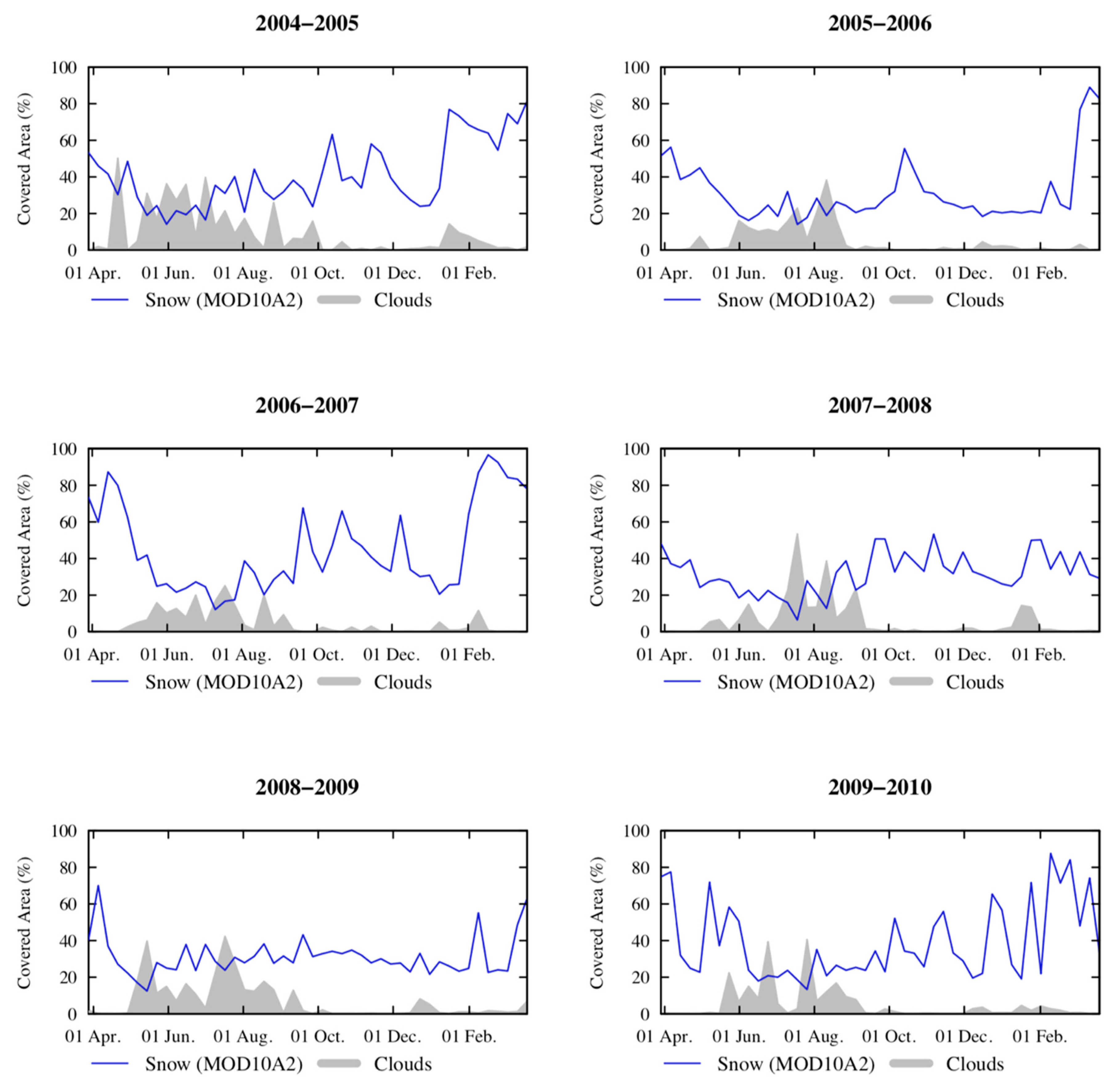
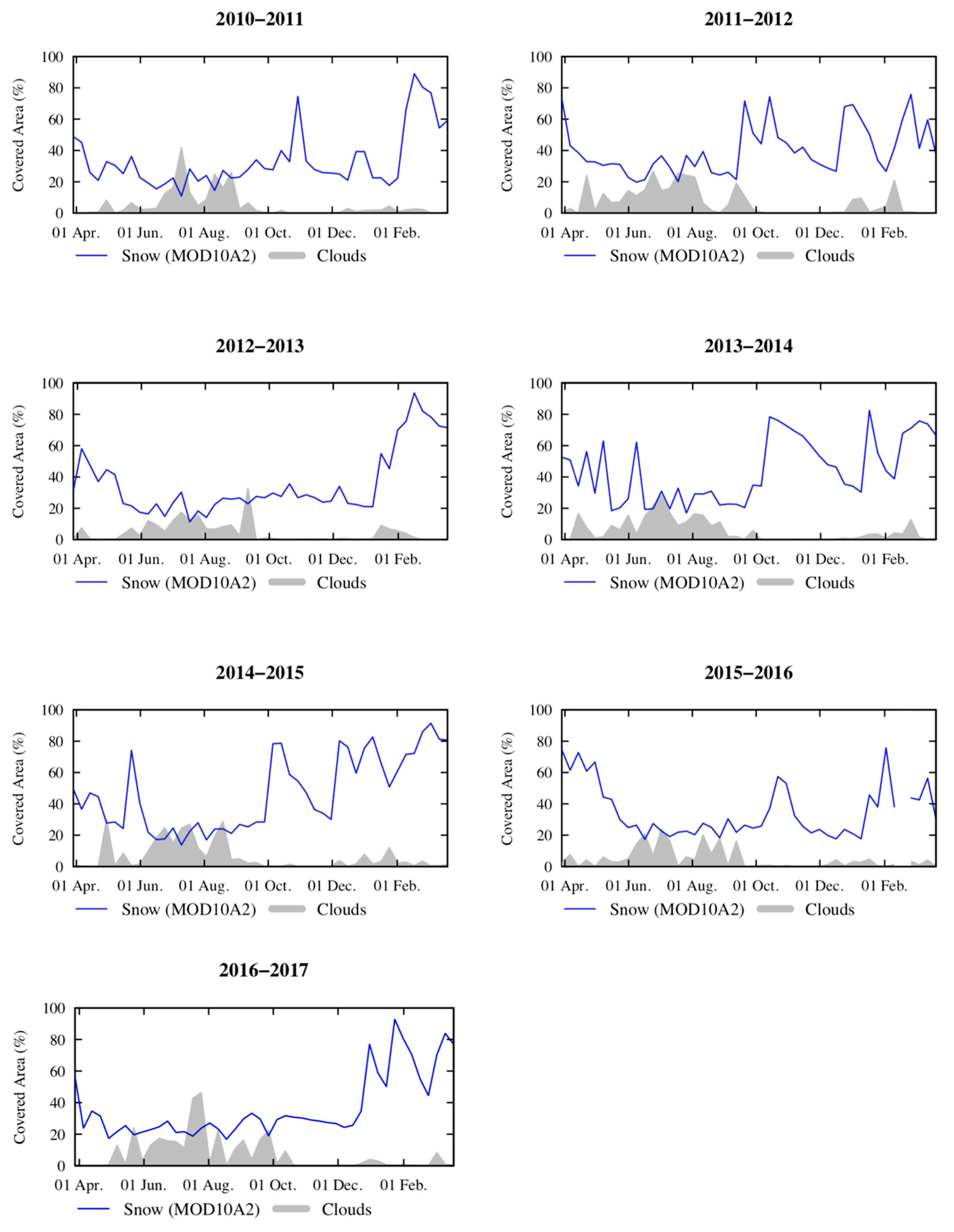
4.1.1. Temporal Evolution of SCA and Cloud Cover

Figure 6 shows the evolution of the SCA from 1998 to 2017 in the Phakding basin. During the 19 years of observation, a slight increase in the SCA for each 8-day interval was observed with Spot-VGT (1998–2000) and MODIS (2000–2017) datasets. However, a Mann–Kendall test run on the time series shows no significant trend, as the p-value largely exceeds 0.05 (p = 0.90). Additional Mann-Kendal tests were also made on the SCA time series that was partitioned in two seasons (October–March and April–September). Even by taking into consideration the seasonality of the dataset, no significant trend was found over the 19-year period for both seasons. The strong variability between winter and summer of the surface energy fluxes that drive snowpack dynamics could explain the general variability of the SCA, and thus, the absence of a significant trend. From this 19-year observation period in 8-day time intervals, it is, therefore, not possible to say that there is monotonic increase in terms of SCA. The low increase may be partly explained by more snowy years, like the year 2015 when the SCA in this area was abnormally high owing to the earthquake that induced the Langtang avalanche [61].

The coherence between snow and cloud-covered surface through the year is shown in Figure 7. The period of the year with the lowest observed SCA (May–September) corresponds to the period with the highest cloud occurrence, as interpreted by the MOD10A2 algorithm. This is also coherent with the hydrological rainy monsoon period in the Himalayas from June to September [62]. The warm monsoon air masses and liquid precipitation in the basin, together with higher longwave radiation budget and warmer night temperatures, lead to a reduction of the SCA in late September, until the beginning of the dry season, with colder temperatures [63]. During summer, the high occurrence of cloud does not naturally reduce the quantity of snow pixels but reduces the amount of snow pixels that is detected by MODIS. It highlights a higher uncertainty of SCA during monsoon period. One study [64] worked on Cloud gap-filling techniques for mapping the snow cover with MODIS and concluded that the gap-filled products have the same uncertainties as the original products. Uncertainties are also greater when there is longer and extended cloud cover period, which is the case for the Nepalese Himalayas during monsoon. Article [30] estimates the error from the 8-day product of MODIS at 8% in cloudy conditions. The error in the present research was likely to be around 8% during summer period.

The high variability of SCA observed during winter (October–March) between the years can be attributed to the high uncertainty of the occurrence of significant snowfall in a year. On the other hand, when a smaller area of the basin is covered by snow, the variation from one year to another is also much smaller. The SCA and the cloud cover area for each year, from 1998 to 2017, are presented in Figure A1.

The hydrological years of 2005–2006, 2007–2008, and 2008–2009 were the years with the lowest annual cumulative SCAs, as opposed to 2006–2007, 2013–2014, and 2014–2015, when the SCAs observed over the watershed were the highest. Both fall seasons of 2013 and 2014 correspond to cyclones Phailin and Hudhud, respectively. These cyclones hit the coast at the Bay of Bengal. The high SCAs observed over the study area in those periods could be attributed to those meteorological events. The difference between years with low SCA and high SCA is noted particularly during the winter months, when the SCA can vary from 50% to 95% between two extreme years (e.g., 2007–2008 versus 2006–2007).

4.1.2. Comparison of MOD10A2 and Ground Measurements

Figure 8 gathers on the same plot, the three sources of data for snowpack description at the location of the Khunde snow plate: (1) the MOD10A2 values for the pixel that contains the Khunde snow plate; (2) the snow depths measured at the snow plate by the observers; (3) the classification of the photos taken by the observers around the snow plate into “no snow,” “partially covered,” and “covered by snow.”

The overall observed dynamics of the snowpack were generally well reproduced by the MOD10A2 product, with maximum volumes and extents occurring between December and April. In addition, for the 2014 and 2015 winter seasons, the date for which MOD10A2 provided snow for that pixel more often corresponded to a photo classified as “covered by snow.” Although the comparison was performed between a 1 km-resolution gridded product and local ground measurements, the good agreement between the MOD10A2 SCA and both the snow depth measurement and the photos of the surrounding area ensures the local reliability of the MOD10A2 product.

4.2. Calibration Results of the Snowmelt Module at the Seasonal Timescale

In order to compare the performances of the one-set and the two-set snowmelt model versions, the SCA was computed as an 8-day output over the 2013–2016 period for both versions of the model and the performances were evaluated in regard to the MO10A2 SCA products. Three different indexes of performance were used: RMSE (km² and %), relative bias (0–1), and the correlation (0–1) with the MOD10A2 products. The simulations that performed the best according to both the RMSE and the bias were computed using the Pareto front method [65]. Figure 9 presents the performances for the ensemble of simulations based on the relative bias and the RMSE for the four sub-basins of this study. The Pareto front is also presented on the right side of Figure 9, for each sub-basin, showing the sets of optimal solutions. Finally, the solution chosen from the Pareto front is highlighted for each basin, for both versions of the snowmelt module, and its index of simulation is indicated above the point.

Table 5. Optimal values for snowmelt parameterization at the seasonal timestep.

Basin	Version	DDF-W	DDF-S	Tm-W	Tm-S	Hmin-W	Hmin-S
		(mm/°C/day)	(mm/°C/day)	(°C)	(°C)	(mm)	(mm)
Pheriche	one-set	14.0		−2.83		6.18
	two-set	13.7	8.6	−3.48	−2.92	6.97	3.99
Dingboche	one-set	3.3		−4.14		6.98
	two-set	16.8	11.1	−3.49	−2.51	6.47	6.63
Tauche	one-set	5.3		−3.31		9.01
	two-set	13.6	6.3	−3.29	−2.40	8.85	5.66
Phakding	one-set	14.0		−1.70		7.30
	two-set	12.4	17.8	−4.70	−1.33	2.57	2.79

presents the optimal solutions chosen for both the one-set and the two-set snowmelt module, as presented in Figure 9. This chosen solution represents the best trade-off between the minimization of both the RMSE and bias. It can be observed that, for the two-set version, the optimal values found for DDF (resp. T_m) are higher (i.e., colder) for the winter season than for the summer season, except for the Phakding basin. This corresponds to a faster snowmelt occurring when the air temperature is above the threshold temperature (T_m). This behavior can be physically explained by considering some of the climatic characteristics of the region: During the summer season, the air is often oversaturated, and the snowpack can contain a significant amount of liquid water, which can lead to snowmelt occurring at a warmer temperature than during winter. Although the model presented here takes little account of the physics of the processes, these considerations show that the differences between winter and summer for the parameterization of the snow process are consistent with the a priori physical knowledge of this environment.

The optimal parameter sets found for each of the four simulated basins significantly differ from one basin to another. This spatial heterogeneity can be explained by the topography of the basins. In particular, the results for the Phakding basin (which includes mid-altitude terrains) show high values for the DDF and T_m during summer, but also a low value of T_m in winter, whereas the Tauche basin (with a south-eastern aspect, particularly submitted to solar radiation) shows high values for the H_min parameter. Greater differences of the parameters DDF and H_min for Tauche can also be explained by the small size of the basin that makes it particularly sensitive and reactive to a slight change in parameters between the two seasons. These results highlight the need for using a spatially-distributed snow parameterization in such contrasted areas. The results are consistent with those from [10] as they are greatly affected by a slight change in the melting threshold temperature (T_m).

Intuitively, high DDF values would lead to a fast snowmelt, low T_m values would lead to a snowmelt at low temperatures (i.e., more frequently during winter), and low H_min values would lead to more snow being considered permanent on the ground. However, additional sensitivity analysis would be necessary to detail the impact of each parameter on the snowpack, depending on the season and on the altitude.

Indeed, this problem remains poorly constrained, with only two indexes for the optimization and six degrees of freedom for the two-set version. The robustness of the optimization method might, thus, be improved by adding additional performance indexes.

5. Discussion

5.1. Impact of the Seasonal Parameterization on SCA modeling

Table 6. Performances of the simulations over the whole year, during winter (October–March), and during summer (April–September) for the two versions of the snowmelt model in the four basins.

Basin	Surface	Obs SCA	Version	Sim SCA	RMSE (%)			Bias (%)			Correlation
	km²	Mean/Surf. Basin		Mean/Surf. Basin	Y	W	S	Y	W	S	Y	W	S
Pheriche	143.9	48.3	one-set	48.6	20.8	24.0	16.9	0.9	8.4	10.5	0.68	0.60	0.62
			two-set	48.3	19.2	23.2	14.4	0.3	6.4	−8.9	0.69	0.61	0.65
Dingboche	145.8	50.8	one-set	50.4	21.9	24.4	18.9	−0.4	3.7	−6.8	0.67	0.63	0.63
			two-set	51.1	20.4	23.6	16.5	1.0	4.6	−4.7	0.68	0.62	0.63
Tauche	4.46	17.7	one-set	17.6	21.7	31.6	18.6	−1.4	7.7	24.7	0.62	0.59	0.56
			two-set	17.6	20.4	28.9	18.8	−1.4	10.5	32.5	0.65	0.63	0.53
Phakding	1218.8	44.5	one-set	44.3	16.9	18.9	14.1	0.1	−5.2	−7.8	0.76	0.73	0.73
			two-set	44.2	15.9	16.7	15.0	−0.5	−6.5	9.3	0.77	0.79	0.59

shows the indexes of performance (RMSE, bias, and correlation) for each basin and for both versions of the snowmelt module with respect to the simulated SCA, on average per basin. The new two-set version of the model improved the RMSE by at least 4% of the total surface of the basin for every case. It is not possible, however, to say that there was a constant improvement in the bias even though the bias remained below 1.4% for each solution. The simulated SCA with the two-set version was also slightly better correlated with the MOD10A2 values compared with the one-set version.

Moreover, Table 6 shows that, according to both the bias and the RMSE criteria, the performances of the simulated SCA were slightly better during winter than during summer. Thus, in the two-set version, the calibration for the summer season can be considered less reliable than the calibration for winter due to higher uncertainty of the SCA measurements from Spot-VGT and MODIS in a prevailing patchy snow cover. However, since the volume of snowfall was less important for all the catchments studied during summer than during winter (see Table 2), the annual performances of the simulated SCA were enhanced at the annual timestep.

By selecting the best combination of sets of parameters for both winter and summer, there was a slight improvement in the simulation of the SCA for the RMSE and the correlation. For both indexes, the yearly performances were enhanced slightly. As shown in Table 6, the major improvement came from the winter period when the snow cover was greater compared with the summer season. Yet, the performances (with respect to the RMSE) may differ between the basins, according to the geographical position and the median elevation of each basin. Indeed, the improvement associated with the two-set version was more significant for the basins located at a higher altitude (i.e., Dingboche and Pheriche basins) in terms of RMSE with regard to the total area of the basin. The Phakding basin showed better results than the other basins regarding the RMSE and the correlation with the MOD10A2 images. Indeed, since the basin covers lower elevation lands (see Figure 2), with less annual snowfall (Figure 3), the total SCA of the Phakding basin is less prone to variation depending on the season.

Figure 10 shows the SCA evolution of the five basins for the years 2013–2016. This figure graphically compares the simulations from the one-set version and the two-set version with the 8-day SCA provided by the MOD10A2. The two-set adaptive threshold (green curve) reduces the offset between the one-set simulated SCA (red curve) and the SCA from the MODIS (blue curve). In particular, for the Phakding basin, the one-set version results seem to underestimate the SCA during summer and to overestimate it during the winter period compared with the MOD10A2 values. This issue is better represented by the two-set version, with a good representation of the dynamics of the simulated SCA on average over this basin. This improvement could be explained by the newly adapted seasonal sets of parameters that were adjusted in accordance with the different meteorological conditions related to the season. However, the method that was proposed reaches a limit when applied to a small basin (i.e., Tauche) and when there is a high variability between winters in terms of precipitation. Winter 2015–2016 had been particularly drier than the three previous winters, and both models (one-set and two-set) missed almost all the events on Tauche during that period. The snow-covered surface observed by MODIS on Tauche in winter 2015–2016 was almost as small as the resolution of the interpolated grid of the model. That explains why the model is likely to represent the basin as completely snow free when a small area is actually covered by snow, according to the sensor.

Both versions of the snowmelt module also show a similar representation of the transition period between winter and summer and fit the observation fairly well. Yearly melting and snow accumulation periods are indeed well depicted during the 2013–2016 period of interest. That confirms that the seasonal adapted model yields improved performances during the summer and winter season without impacting the performances of the initial model during the transition periods.

Even with the slight enhancement of the simulated SCA brought about by the two-set version of the snowmelt module, there is still a gap in the representation of strong accumulation of snow followed directly by an important melting event during the same period. In the improved version, since only two sets of parameters represent the whole study period, it still remains a coarse depiction of the actual accumulation–melt dynamics in such a high mountainous terrain. Even if the two-set snowmelt module presents better representation of MODIS SCA during winter and monsoon than the one-set version, the model still struggles to correctly represent the transition periods and strong weather changes within the seasons that are characterized extreme snow cover fluctuations. Further tests were conducted with an additional set of parameters for the transition periods (April–May and October–November), but no clear improvement of the simulated SCA was observed during transition periods. That seems to indicate that even by increasing the number of parameter sets, the simple degree day model reaches a limit in representing the snowmelt. More physically-based models of snow may, therefore, be required for a better characterization of the melting of snow at this point. Other biases that could alter the quality of the results are the error on the observations from MODIS and the undercatch of solid precipitation under windy conditions [66,67] that affects the values of interpolated precipitation maps. A validation of the degree day snowmelt model along with MOD10A2 products in a different terrain would also be required to confirm the quality of this method, its versatility, and its reproducibility.

5.2. Impact of the Seasonal Parameterization on Snowmelt Modeling

Table 7. Annual volumes of simulated snowmelt using (A) the one-set and (B) the two-set version of the snow model. The percentages are those values divided by the annual observed discharge.

Basin	2013–2014		2014–2015		2015–2016
	mm—(%)		mm—(%)		mm—(%)
	one-set	two-set	one-set	two-set	one-set	two-set
Pheriche	393—(50)	388—(49)	426—(41)	419—(40)	386—(46)	363—(44)
Dingboche	507—(65)	477—(62)	461—(37)	466—(37)	467—(51)	415—(46)
Tauche	275—(64)	278—(64)	268—(58)	296—(61)	218—(62)	188—(59)
Phakding	392—(49)	384—(48)	386—(33)	407—(35)	353—(40)	296—(33)

presents the annual volumes of simulated snowmelt using the one-set and the two-set versions of the snow model, together with the percentages of those values divided by the annual observed discharge. The introduction of the two-set version appears to reduce the contribution of snowmelt to discharge by less than 1–7%. This can be explained by the fact that the two-set version allows us to increase the simulated SCA during winter (see Section 3.3), which is the season with the highest amount of snowfall. Moreover, the values of runoff from snowmelt simulated with the two-set version are consistent with the previous works that have been conducted for these same catchments by [21,68].

This behavior was observed for all the basins and all the years, expect for the Phakding and the Tauche basin during 2014–2015, for which the two-set version provided a higher snow contribution than the one-set version. This particular behavior can be related to a particular meteorological event that occurred in March 2015 (i.e., during summer season), leading to an extreme amount of solid precipitation at mid-altitudes.

In summary, the introduction of the two-set version of the snow model parameterization allows us to enhance the simulation of the SCA with regard to the MOD10A2 SCA, with conservation of the annual snowmelt amounts in accordance with the literature values.

6. Conclusions

The aim of this study was to utilize the long time series of remote sensing datasets to enhance the parameterization of the seasonal variability of snow processes in a snow model based on the degree day method. Four watersheds located in the northern part of the northern Dudh Koshi watershed, Nepal, were studied in this work.

Both the SPOT-VGT and the MODIS datasets were combined in order to implement a database of snow cover area (SCA) maps with an 8-day timestep over the northern part of the Dudh Koshi watershed for the 1987–2016 period. Here, a simple threshold-based approach was applied to the SPOT-VGT and MODIS datasets in order to create binary snow maps, based on the NDSI index for snow detection. This processed SCA product was compared with local field measurements performed from 2012 to 2016. The overall dynamics of the snowpack observed were generally well reproduced by the MODIS product, with maximum volumes and extents occurring between December and April.

The corrected remote sensing images show the high spatial and seasonal variability of the SCA and they highlight the challenges of representing the seasonal variability of snow processes in this region. These modeling issues offered the opportunity to implement a new version of the degree day snow module of the HDSM model, in order to partition it into two parameterizations depending on the seasonality. Nevertheless, it should be noted that hydrological modeling is not discussed in the current article and will be the subject of an upcoming paper, which is in the stage of finalization. The corrected 8-day MODIS SCA maps were then used to calibrate the parameters of the snow module of the HDSM model, through a stochastic method, either with the annual or the seasonal timestep. From there, the performances of the model parameterization when using one annual parameter set (one-set version) or when introducing one parameterization for each of the two seasons (two-set version) were compared, regarding the representation of the SCA of the four watersheds, compared with the 8-day MODIS images. The results show that the two-set parameterization significantly reduces the error in the simulated SCA compared with the MODIS SCA. However, this poorly constrained problem presents a high degree of equifinality.

The impacts of the two-set parameterization on the simulation of SCA and snowmelt fluxes were analyzed. The results show that, at the annual timescale, the new two-set version of the model improves the simulation of the SCA with regard to the MODIS values, compared with the one-set version. However, owing to cloud coverage affecting the MODIS remote data during summer, in the two-set version, the calibration for the summer season can be considered less reliable than the calibration for winter.

In conclusion, this study shows that the use of remote sensing products can significantly enhance the parameterization of the seasonal dynamics of snow processes in a model based on a degree day method. Furthermore, adapting the degree day model with two sets of parameters increases the performance of the model. An extended validation of the method could be performed over a different terrain or over a different period. Finally, it may be of great interest to link this representation of the seasonal variability of the snow processes to the current estimation of climate change impacts in this region. Indeed, the expected change in the timing of the Asian monsoon could significantly influence the snowmelt timing in the Himalayan region [11].

References

1. IPCC. Climate Change 2013: The Physical Science Basis. Contribution of Working Group I to the Fifth Assessment Report of the Intergovernmental Panel on Climate Change; Stocker, T.F., Qin, D., Plattner, G.-K., Tignor, M., Allen, S.K., Boschung, J., Nauels, A., Xia, Y., Bex, V., Midgley, P.M., Eds.; Cambridge University Press: Cambridge, UK; New York, NY, USA, 2013; p. 1535. [Google Scholar]
2. Allen, M.; Babiker, M.; Chen, Y.; de Coninck, H.; Connors, S.; van Diemen, R.; Dube, O.P.; Ebi, K.L.; Engelbrecht, F.; Ferrat, M.; et al. Global warming of 1.5 C, summary for policy makers. Intergov. Panel Clim. Chang. 2018, 6, 32. [Google Scholar]
3. Lutz, A.F.; Immerzeel, W.W.; Shrestha, A.B.; Bierkens, M.F.P. Consistent increase in High Asia’s runoff due to increasing glacier melt and precipitation. Nat. Clim. Chang. 2014, 4, 587. [Google Scholar] [CrossRef]
4. Armstrong, R.L.; Rittger, K.; Brodzik, M.J.; Racoviteanu, A.; Barret, A.P.; Khalsa, S.-J.; Raup, B.; Hill, A.; Khan, A.; Wilson, A.; et al. Runoff from glacier ice and seasonal snow in High Asia: Separating melt water sources in river flow. Reg. Environ. Chang. 2019, 19, 1249–1261. [Google Scholar] [CrossRef]
5. Quincey, D.; Klaar, M.; Haines, D.; Lovett, J.; Pariyar, B.; Gurung, G.; Brown, L.; Watson, C.; England, M.; Evans, B. The changing water cycle: The need for an integrated assessment of the resilience to changes in water supply in High-Mountain Asia. WIREs Water 2018, 5, e1258. [Google Scholar] [CrossRef]
6. Kraaijenbrink, P.D.A.; Bierkens, M.F.P.; Lutz, A.F.; Immerzeel, W.W. Impact of a global temperature rise of 1.5 degrees Celsius on Asia’s glaciers. Nature 2017, 549, 257. [Google Scholar] [CrossRef]
7. Pritchard, H.D. Asia’s glaciers are a regionally important buffer against drought. Nature 2017, 545, 169. [Google Scholar] [CrossRef]
8. Bookhagen, B.; Burbank, D.W. Toward a complete Himalayan hydrological budget: Spatiotemporal distribution of snowmelt and rainfall and their impact on river discharge. J. Geophys. Res. Earth Surf. 2010, 115. [Google Scholar] [CrossRef] [Green Version]
9. Dhar, O.N.; Rakhecha, P.R. The effect of elevation on monsoon rainfall distribution in the central Himalayas. In Monsoon Dynamics, 1st ed.; Cambridge University Press: Cambridge, UK, 1981; pp. 253–260. [Google Scholar]
10. Savéan, M.; Delclaux, F.; Chevallier, P.; Wagnon, P.; Gonga-Sholiariliva, N.; Sharma, R.; Neppel, L.; Arnaud, Y. Water budget on the Duth Koshi river (Nepal): Uncertainties on precipitation. J. Hydrol. 2015, 531, 850–862. [Google Scholar] [CrossRef]
11. Bajracharya, A.R.; Bajracharya, S.R.; Shreshta, A.B.; Maharjan, S.B. Climate change impact assessment on the hydrological regime of the Kaligandaki Basin, Nepal. Sci. Total Environ. 2018, 625, 837–848. [Google Scholar] [CrossRef]
12. Immerzeel, W.W.; van Beek, L.P.; Bierkens, M.F. Climate change will affect the Asian water towers. Science 2010, 328, 1382–1385. [Google Scholar] [CrossRef]
13. Andermann, C.; Longuevergne, L.; Bonnet, S.; Crave, A.; Davy, P.; Gloaguen, R. Impact of transient groundwater storage on the discharge of Himalayan rivers. Nat. Geosci. 2012, 5, 127. [Google Scholar] [CrossRef]
14. Ragettli, S.; Pellicciotti, F. Calibration of a physically based, spatially distributed hydrological model in a glacierized basin: On the use of knowledge from glaciometeorological processes to constrain model parameters. Water Resour. Res. 2012, 48. [Google Scholar] [CrossRef]
15. Nepal, S.; Flügel, W.A.; Shrestha, A.B. Upstream-downstream linkages of hydrological processes in the Himalayan region. Ecol. Process. 2014, 3, 1–19. [Google Scholar] [CrossRef]
16. Pokhrel, B.K.; Chevallier, P.; Andréassian, V.; Tahir, A.A.; Arnaud, Y.; Neppel, L.; Bajracharya, O.R.; Budhathoki, K.P. Comparison of two snowmelt modelling approaches in the Dudh Koshi basin (eastern Himalayas, Nepal). Hydrolog. Sci. J. 2013, 59, 1507–1518. [Google Scholar] [CrossRef]
17. Bharati, L.; Gurung, P.; Maharjan, L.; Bhattarai, U. Past and future variability in the hydrological regime of the Koshi Basin, Nepal. Hydrolog. Sci. J. 2016, 61, 79–93. [Google Scholar] [CrossRef]
18. Martinec, J. Snowmelt—Runoff model for stream flow forecasts. Hydrol. Res. 1975, 6, 145–154. [Google Scholar] [CrossRef]
19. Dey, B.; Sharma, V.K.; Rango, A. A test of snowmelt-runoff model for a major river basin in western Himalayas. Nord. Hydrol. 1989, 20, 167–178. [Google Scholar] [CrossRef]
20. Savéan, M. Modélisation Hydrologique Distribuée et Perception de la Variabilité Hydro-Climatique par la Population du Bassin Versant de la Dudh Koshi (Népal). Ph.D. Thesis, Université Montpellier 2, Montpellier, France, 31 October 2014. [Google Scholar]
21. Eeckman, J.; Nepal, S.; Chevallier, P.; Camensuli, G.; Delclaux, F.; Boone, A.; De Rouw, A. Comparing the ISBA and J2000 approaches for surface flows modelling at the local scale in the Everest region. J. Hydrol. 2019, 569, 705–719. [Google Scholar] [CrossRef]
22. DeWalle, D.R.; Rango, A. Principle of Snow Hydrology; Cambridge University Press: New York, NY, USA, 2008; p. 410. [Google Scholar]
23. Parajka, J.; Blösch, G. Validation of MODIS snow cover images over Austria. Hydrol. Earth Syst. Sci. Discuss. 2006, 10, 679–689. [Google Scholar] [CrossRef] [Green Version]
24. Painter, T.H.; Rittger, K.; McKenzie, C.; Slaughter, P.; Davis, R.E.; Dozier, J. Retrieval of subpixel snow covered area, grain size, and albedo from MODIS. Remote Sens. Environ. 2009, 113, 868–879. [Google Scholar] [CrossRef] [Green Version]
25. Sirguey, P.; Mathieu, R.; Arnaud, Y. Subpixel monitoring of the seasonal snow cover with MODIS at 250 m spatial resolution in the Southern Alps of New Zealand: Methodology and accuracy assessment. Remote Sens. Environ. 2009, 113, 160–181. [Google Scholar] [CrossRef]
26. Gascoin, S.; Hagolle, O.; Huc, M.; Jarlan, L.; Dejoux, J.F.; Szczypta, C.; Marti, R.; Sanchez, R. A snow cover climatology for the Pyrenees from MODIS snow products. Hydrol. Earth Syst. Sci. 2015, 19, 2337–2351. [Google Scholar] [CrossRef] [Green Version]
27. Masson, T.; Dumont, M.; Dalla-Mura, M.; Sirguey, P.; Gascoin, S.; Dedieu, J.P.; Chanussot, J. Assessment of existing methodologies to retrieve snow cover fraction from MODIS data. Remote Sens. 2018, 10, 619. [Google Scholar] [CrossRef]
28. McCabe, M.F.; Rodell, M.; Alsdorf, D.E.; Miralles, D.G.; Uijlenhoet, R.; Wagner, W.; Lucieer, A.; Houborg, R.; Verhoest, N.E.C.; Franz, T.E.; et al. The future of Earth observation in hydrology. Hydrol. Earth Syst. Sci. 2017, 21, 3879–3914. [Google Scholar] [CrossRef] [PubMed] [Green Version]
29. Dozier, J.; Painter, T. Multispectral and hyperspectral remote sensing of alpine snow properties. Annu. Rev. Earth Planet Sci. 2004, 32, 465–494. [Google Scholar] [CrossRef]
30. Parajka, J.; Blöschl, G. Spatio-temporal combination of MODIS images–potential for snow cover mapping. Water Resour. Res. 2008, 44. [Google Scholar] [CrossRef]
31. Notarnicola, C.; Duguay, M.; Moelg, N.; Schellenberger, T.; Tetzlaff, A.; Monsoro, R.; Costa, A.; Steurer, C.; Zebisch, M. Snow cover maps from MODIS images at 250 m resolution, Part 1: Algorithm description. Remote Sens. 2013, 5, 110–126. [Google Scholar] [CrossRef]
32. Dedieu, J.P.; Lessard-Fontaine, A.; Ravazzani, G.; Cremonese, E.; Shalpykova, G.; Beniston, M. Shifting mountain snow patterns in a changing climate from remote sensing retrieval. Sci. Total Environ. 2014, 493, 1267–1279. [Google Scholar] [CrossRef] [Green Version]
33. Hüsler, F.; Jonas, T.; Riffler, M.; Musial, J.P.; Wunderle, S. A satellite-based snow cover climatology (1985–2011) for the European Alps derived from AVHRR data. Cryosphere 2014, 8, 73–90. [Google Scholar] [CrossRef]
34. Notarnicola, C.; Mölg, N.; Rastner, P.; Irsara, L.; Zebnisch, M. Monitoring snow cover changes in the Alpine Regions through MODIS and LANDSAT time series. In Proceedings of the International Mountain Conference, Perth, UK, 26–30 September 2010; pp. 786–787. [Google Scholar]
35. Racoviteanu, A.E.; Armstrong, R.; Williams, M.W. Evaluation of an ice ablation model to estimate the contribution of melting glacier ice to annual discharge in the Nepal Himalaya. Water Resour. Res. 2013, 49, 5117–5133. [Google Scholar] [CrossRef]
36. Rabus, B.; Eineder, M.; Roth, A.; Bamler, R. The shuttle radar topography mission—A new class of digital elevation models acquired by spaceborne radar. ISPRS J. Photogramm. Remote Sens. 2003, 57, 241–262. [Google Scholar] [CrossRef]
37. Eeckman, J.; Chevallier, P.; Boone, A.; Neppel, L.; De Rouw, A.; Delclaux, F.; Koirala, D. Providing a non-deterministic representation of spatial variability of precipitation in the Everest region. Hydrol. Earth Syst. Sci. 2017, 21, 4879–4893. [Google Scholar] [CrossRef] [Green Version]
38. Barry, R.G. Mountain Weather and Climate, 3rd ed.; Cambridge University Press: Cambridge, UK, 2008; p. 506. [Google Scholar]
39. Valery, A.; Andreassian, V.; Perrin, C. Regionalization of precipitation and air temperature over high-altitude catchments learning from outliers. Hydrol. Sci. J. 2010, 55, 928–940. [Google Scholar] [CrossRef]
40. Lafaysse, M.; Hingray, B.; Etchevers, P.; Martin, E.; Obled, C. Influence of spatial discretization, underground water storage and glacier melt on a physically-based hydrological model of the Upper Durance River basin. J. Hydrol. 2011, 403, 116–129. [Google Scholar] [CrossRef]
41. Gottardi, F.; Obled, C.; Gailhard, J.; Paquet, E. Statistical reanalysis of precipitation fields based on ground network data and weather patterns: Application over french mountains. J. Hydrol. 2012, 432, 154–167. [Google Scholar] [CrossRef]
42. Burns, J.I. Small-scale topographic effects on precipitation distribution in San Dimas experimental forest. Eos Trans. Am. Geophys. Union 1953, 34, 761–768. [Google Scholar] [CrossRef]
43. Alpert, P. Mesoscale indexing of the distribution of orographic precipitation over high mountains. J. Clim. Appl. Meteorol. 1986, 25, 532–545. [Google Scholar] [CrossRef]
44. L’Hôte, Y.; Chevallier, P.; Coudrain, A.; Lejeune, Y.; Etchevers, P. Relationship between precipitation phase and air temperature: Comparison between the Bolivian Andes and the Swiss Alps. Hydrol. Sci. J. 2005, 50, 989–997. [Google Scholar]
45. Armstrong, R.L.; Brun, E. Snow and Climate: Physical Processes, Surface Energy Exchanges and Modeling; Cambridge University Press: Cambridge, UK, 2010; p. 256. [Google Scholar]
46. Wiscombe, W.J.; Warren, S.G. A model for the spectral albedo of snow. I—Pure snow. J. Atmos. Sci. 1980, 37, 2712–2733. [Google Scholar] [CrossRef]
47. Warren, S.G. Optical properties of snow. Rev. Geophys. 1982, 20, 67–89. [Google Scholar] [CrossRef]
48. Rees, W.G. Remote Sensing of Snow and Ice; Taylor & Francis: Abingdon, UK; CRC Press Book: Cambridge, UK, 2006; p. 285. [Google Scholar]
49. Dozier, J. Spectral signature of alpine snow cover from the Landsat Thematic Mapper. Remote Sens. Environ. 1989, 28, 9–22. [Google Scholar] [CrossRef]
50. Sergent, C.; Coléou, C.; David, P. Mesures Nivo-Météorologiques. Document de Formation des Pisteurs Secouristes 2eme Degré; CNRM, CEN, Météo France: Grenoble, France, 1996. [Google Scholar]
51. Gascoin, S.; Dubertret, F.; Drapeau, L.; Gonga-Saholiariliva, N.; Jarlan, L.; Duchemin, B.; Maisongrande, P. SCoTA: An open source toolbox for snow cover mapping from SPOT-VEGETATION daily syntheses. In Proceeding of the International Geoscience and Remote Sensing Symposium, Quebec City, QC, Canada, 13–18 July 2014. [Google Scholar]
52. Lissens, G.; Kempeneers, P.; Fierens, F.; Van Rensbergen, J. Development of cloud, snow, and shadow masking algorithms for VEGETATION imagery. In Proceedings of the IEEE IGARSS Taking the Pulse of the Planet: The Role of Remote Sensing in Managing the Environment, Honolulu, HI, USA, 24–28 July 2000. [Google Scholar]
53. Berthelot, B. Snow Detection on VEGETATION Data—Improvement of Cloud Screening; No. NOV-3128-NT-2295, v1.1, 54 p., VITO, Be; VITO: Mol, Belgium, 2004. [Google Scholar]
54. Irish, R.; Barker, J.; Goward, S.; Arvidson, T. Characterization of the Landsat-7 ETM+ automated Cloud-Cover Assessment (ACCA) algorithm. Photogramm. Eng. Remote Sens. 2006, 72, 1179–1188. [Google Scholar] [CrossRef]
55. Hall, D.K.; Riggs, G.A.; Salomonson, V.V. Development of methods for mapping global snow cover using moderate resolution imaging spectroradiometer data. Remote Sens. Environ. 1995, 54, 127–140. [Google Scholar] [CrossRef]
56. Hall, D.K.; Riggs, G.A.; Salomonson, V.V.; DiGirolamo, N.E.; Bayr, K.J. MODIS snow-cover products. Remote Sens. Environ. 2002, 83, 181–194. [Google Scholar] [CrossRef] [Green Version]
57. Riggs, G.A.; Hall, D.K.; Román, M.O. Overview of NASA’s MODIS and VIIRS snow-cover earth system data records. Earth Syst. Sci. 2017, 9, 765–777. [Google Scholar] [CrossRef]
58. Wang, X.; Xie, H.; Liang, T. Evaluation of MODIS snow cover and cloud mask and its application in Northern Xinjiang, China. Remote Sens. Environ. 2008, 112, 1497–1513. [Google Scholar] [CrossRef]
59. Riggs, G.A.; Hall, D.K. Modis Snow Products Collection 6 User Guide; National Snow and Ice Data Center: Boulder, CO, USA, 2015; p. 66. [Google Scholar]
60. MacKay, M.D.; Beckman, R.J.; Conover, W.J. A comparison of three methods for selecting values of input variables in the analysis of output from a computer code. Technometrics 2000, 42, 55–61. [Google Scholar] [CrossRef]
61. Fujita, K.; Inoue, H.; Izumi, T.; Yamaguchi, S.; Sadakane, A.; Sunako, S.; Nishimura, K.; Immerzeel, W.; Shea, J.M.; Kayastha, R.B.; et al. Anomalous winter-snow-amplified earthquake-induced disaster of the 2015 Langtang avalanche in Nepal. Nat. Hazards Earth Syst. 2017, 17, 749–764. [Google Scholar] [CrossRef] [Green Version]
62. Neupane, R.; White, J.; Alexander, S. Projected hydrologic changes in monsoon-dominated Himalaya mountain basins with changing climate and deforestation. J. Hydrol. 2015, 525, 216–230. [Google Scholar] [CrossRef]
63. Ménégoz, M.; Gallée, H.; Jacobi, H.W. Precipitation and snow cover in the Himalaya: From reanalysis to regional climate simulations. Hydrol. Earth Syst. Sci. 2013, 17, 3921–3936. [Google Scholar] [CrossRef]
64. Hall, D.K.; Riggs, G.A. DiGirolamo, N.E.; Roman, M.O. MODIS cloud-gap filled snow-cover products: Advantages and uncertainties. Hydrol. Earth Syst. Sci. Discuss. 2019. in review. [Google Scholar] [CrossRef]
65. Coello, C.A.C. Recent trends in evolutionary multiobjective optimization. In Evolutionary Multiobjective Optimization; Springer: London, UK, 2005; pp. 7–32. [Google Scholar]
66. Sevruk, B. International workshop on precipitation measurement I: Preface. Hydrol. Process. 1991, 5, 229–232. [Google Scholar] [CrossRef]
67. Rasmussen, R.; Baker, B.; Kochendorfer, J.; Meyers, T.; Landolt, S.; Fischer, A.P.; Black, J.; Theriault, J.; Kucera, P.; Gochis, D.; et al. How well are we measuringsnow: The NOAA/FAA/NCAR winter precipitation test bed. Bull. Am. Meteorol. Soc. 2012, 93, 811–829. [Google Scholar] [CrossRef]
68. Mimeau, L. Quantification des Contributions Aux Écoulements Dans un Bassin Englacé par Modélisation Glacio-Hydrologique: Application à un Sous-Bassin de la Dudh Koshi (Népal, Himalaya). Ph.D. Thesis, IGE—Institut des Géosciences de l’Environnement, Grenoble, France, 29 August 2018. [Google Scholar]
Figure 1. Study area. Left: the northern part (blue limits) of the Dudh Koshi River basin (red limits). Right: the sub-basins studied: Pheriche (orange limits), Dingboche (yellow limits), Tauche (green limits), and Phakding (blue limits). Source: SRTM (Shuttle Radar Topography Mission) digital elevation map [36].
Remotesensing 11 02598 g001
Figure 2. Hypsometric curve of Phakding, Pheriche, and the northern part of the Dudh Koshi River basin and the elevation of the meteorological stations. Source: SRTM (Shuttle Radar Topography Mission) digital elevation map [36].
Remotesensing 11 02598 g002
Figure 3. Maps of the average total and solid precipitation and the air temperature for the river basins studied over the period 2013–2016. Values are given for the total area of the basins, including the glaciated areas.
Remotesensing 11 02598 g003
Figure 4. Snapshot examples of snow cover extent and height measurements at the Khunde site.
Remotesensing 11 02598 g004
Figure 5. Operating diagram of the snowmelt model for the “all-year” version (A) and for the “two-season” version (B). The indexes “W” and “S” are used, respectively, to identify the parameters for the winter and the summer period for the two-season version.
Remotesensing 11 02598 g005
Figure 6. Temporal evolution of snow cover area (SCA) in the Phakding basin from the Spot-VGT and MOD10A2 dataset (1998–2017).
Remotesensing 11 02598 g006
Figure 7. Intra-annual variation of 8-day synthesis of snow cover and cloud coverage in the Phakding basin (mean values 1998–2017). The standard deviation of the snow cover area between the years is also presented.
Remotesensing 11 02598 g007
Figure 8. Three sources of data for snowpack description at the location of the Khunde snow plate between December 2012 and July 2015: (1) in black lines, the snow depths (in cm) measured at the snow plate by the observers; (2) in blue, the photos taken by the observers around the snow plate classified as “no snow” (light blue), “partially covered,” and “covered by snow” (dark blue). No blue bar means that no photo was taken for these dates. The red bars indicate the MOD10A2 dates for which the pixel that contains the Khunde snow plate was determined to be covered by snow.
Remotesensing 11 02598 g008
Figure 9. Performances of the simulated SCA. The data used as references were the processed MOD10A2 SCA. The left part of the figure shows all the simulations for the four sub-basins inside the solution area (RMSE and relative bias). The right part shows a closer view of the most performant solutions for each basin. The dots represent the Pareto front and the stars indicate the selected solution.
Remotesensing 11 02598 g009
Figure 10. Evolution of simulated SCA, with the “one-set” (red line) and the “two-set” (green line) version of the snowmelt model, along with the 8-day SCA provided by MOD10A2 (blue line), on average per basin, for the five basins during the 2013–2016 period. The summer seasons are highlighted in gray.
Remotesensing 11 02598 g010