Article

Processing of VENµS Images of High Mountains: A Case Study for Cryospheric and Hydro-Climatic Applications in the Everest Region (Nepal)

1
Geo-Ocean Laboratory (LGO), University Brest, CNRS, Ifremer, UMR 6538, 29280 Plouzané, France
2
LETG-Brest, University Brest, CNRS, UMR 6554, 29280 Plouzané, France
3
Institute for Geosciences and Environmental Research (IGE), University Grenoble-Alpes/CNRS/IRD/Grenoble-INP, 38058 Grenoble, France
4
Department of Geography and Planning, Appalachian State University, Boone, NC 28608, USA
5
Department of Geography, King’s College London, London WC2B 4BG, UK
*
Author to whom correspondence should be addressed.
These authors contributed equally to this work.
Remote Sens. 2022, 14(5), 1098; https://doi.org/10.3390/rs14051098
Submission received: 23 December 2021 / Revised: 18 February 2022 / Accepted: 19 February 2022 / Published: 23 February 2022
(This article belongs to the Special Issue VENµS Image Processing Techniques and Applications)

Abstract

:
In the Central Himalayas, glaciers and snowmelt play an important hydrological role, as they ensure the availability of surface water outside the monsoon period. To compensate for the lack of field measurements in glaciology and hydrology, high temporal and spatial resolution optical remotely sensed data are necessary. The French–Israeli VENµS Earth observation mission has been able to complement field measurements since 2017. The aim of this paper is to evaluate the performance of different reflectance products over the Everest region for constraining the energy balance of glaciers and for cloud and snow cover mapping applied to hydrology. Firstly, the results indicate that a complete radiometric correction of slope effects such as the Gamma one (direct and diffuse illumination) provides better temporal and statistical metrics (R2 = 0.73 and RMSE = 0.11) versus ground albedo datasets than a single cosine correction, even processed under a fine-resolution digital elevation model (DEM). Secondly, a mixed spectral-textural approach on the VENµS images strongly improves the cloud mapping by 15% compared with a spectral mask thresholding process. These findings will improve the accuracy of snow cover mapping over the watershed areas downstream of the Everest region.

1. Introduction

1.1. Context

Hosting the highest mountains in the world and the largest glacierized area outside of the polar regions, the Himalayas are a unique hydro-climatic system. The numerous Himalayan watersheds supply more than 800 million people downstream, providing water resources from 760,000 km2 of snow-covered areas and 40,800 km2 of glaciers (including Karakoram and the Himalayas). Therefore these high mountains are often called “water towers” for the buffering role they play in the Asian water cycle [1,2,3] with snow and ice melt maintaining streamflow during periods of meteorological drought [3,4,5]. However, this region is a challenge for high-elevation glacio-hydrologic research. Distributed hydro-meteorological information is limited by the difficulty of collecting in situ data [6], translating into limited knowledge of the hydrological regime and its evolution. Gridded meteorological data are available in mountain areas (e.g., ERA5 [7] or HAR [8] climate reanalysis) but they remain too coarse to directly resolve processes in mountain catchments. Their performance on a larger scale in mountainous regions is also often unknown, again due to the lack of sufficiently dense observational networks. These limitations create considerable uncertainty about the future evolution of the Himalayan Water Towers [9,10].
The increasing resolution of spaceborne sensors and the lengthening of available time series means that optical remote sensing is offering new opportunities to fill the data gap, by up-scaling in situ measurements at the basin scale, and/or by monitoring unsurveyed regions. This is especially true in the field of snow monitoring [11]. For example, in the Everest region, MODIS (Moderate-Resolution Imaging Spectroradiometer) imagery has been used to help constrain the contributions of snow and ice to streamflow [12,13,14] and to track seasonal migration of the snow line [15]. A new technical step was reached in terms of spatio-temporal resolution with the Copernicus Sentinel platforms from ESA (European Space Agency), and the recent VENµS (Vegetation and Environment New Micro Satellite) program.

1.2. Advantages of VENµS Reflectance Products

The VENµS micro satellite mission is jointly developed and managed by the French Space Agency (CNES) and the Israeli Space Agency (ISA). Since August 2017, VENµS sun-synchronous sensor has provided optical images every 2 days from 12 narrow spectral bands from blue visible (0.424 µm) to near-infrared (0.910 µm), with a 5 m ground resolution. For our study area, the registration time is 11:00 local time. The VENµS program aims to highlight the benefits of repetitive high-resolution image acquisitions for monitoring land surface dynamics. With its unique high spatio-temporal resolution characteristics, the VENµS sensor is well suited to snow monitoring, particularly in high mountain areas that are difficult to access. A total of 130 experimental sites worldwide were selected for the VM1 (VENµS Mission 1) step program (2017–2020), including Mount Everest and the Khumbu valley in Nepal for this study (KHUMBU tile, “Pointing” project). L1C (Level 1C, single date ortho-rectified image expressed in top-of-atmosphere reflectance) and L2A (Level 2A, single date ortho-rectified image expressed in surface reflectance) images are processed by CNES (MAJA chain [16]) providing surface reflectance (SRE) and flat reflectance (FRE) output products, distributed by the THEIA site [17]. The 90 m SRTM (Shuttle Radar Topography Mission) DEM is used by CNES to compute the FRE product with topographic and radiometric corrections using the Gamma process [18,19]. In this way, CNES offers a very high-quality reflectance product with a high revisit frequency and spatial resolution. However, the 8 m HMA (High Mountain Asia) DEM is available in the Khumbu region and could be used to apply the slope effect correction in place of the 90 m SRTM DEM. Thus, we could analyze the influence of the DEM resolution on the topographic correction.

1.3. Snow and Cloud Discrimination in Optical Remote Sensing

Concerning the question of snow cover changes at a regional scale adapted to mountainous watersheds, long-term databases offer regular snow map collection (albedo, Snow Cover Area (SCA)); i.e., the National Snow and Ice Data Center (NSIDC) [20] or the Copernicus Snow and Ice Monitoring Service [21]. For this purpose, different methods have been developed to compute changes in terms of the snow cover duration (SCD in days) and snow cover area (in km2). A complete review is given by [22]. The most efficient method to separate clouds and snow is given by the NDSI (Normalized-Difference Snow Index) [23] based on the normalized ratio between Green and SWIR (Short-Wave Infrared) spectral bands:
N D S I = R g r e e n R s w i r R g r e e n + R s w i r
where R g r e e n is the surface reflectance in the green spectral band and R s w i r is the surface reflectance in the SWIR (1.6 µm) spectral band. Indeed, snow has a very low reflectance in the SWIR band [24]. Mainly based on the NDSI method, MODIS datasets at regional scale have been widely used [25,26,27,28,29], as well as Sentinel-2 and -3 products [30,31] to compute SCD and SCA. Unlike Sentinel-2 images, the lack of 1.6 µm SWIR spectral band on the VENµS sensor prevents direct snow and ice mapping through the NDSI calculation [28]; thus, alternative methods are needed. Only a few studies have already addressed this issue in other sensors. A method has been developed on Worldview-2 sensor by Bühler et al. [32] using the visible and the highest NIR (Near Infra-Red) band in a normalized-difference band ratios index. It should be noted that no atmospheric or radiometric correction has been applied to these satellite images. In Marchane et al. [33], they apply a supervised classification using the parallelepiped approach with the green, red and NIR bands of the FORMOSAT-2 sensor to retrieve the snow cover. Recently, to overcome this constraint with VENµS, Baba & Gascoin [34] suggested an approach using VENµS database (named the NDSIµ index), based on the Red-edge and NIR spectral bands with classification method for SCA mapping in mountainous environments. However, the 15 FORMOSAT-2 images used in Marchane et al. had almost no clouds, which avoids the difficulty of differentiating snow and cloud. Baba & Gascoin [34] used the VENµS cloud mask to exclude clouds in the process. Therefore, the discrimination between snow and clouds remains unaddressed.
Cloud cover is a major constraint in optical remote sensing, impacting the retrieval of surface properties. Different masking algorithms exist, based on multi-temporal or elevation methods [35,36] but spectral similarity between cloud and snow can be challenging [37,38]. Most solutions developed recently to detect clouds in remote-sensed images involve machine learning or deep learning methods [39,40,41,42] using convolutional neural network architectures. Although these methods offer attractive results, the implementation of such a process requires considerable computing resources and is often time consuming. We intend to propose here a simple and parsimonious alternative. Generally, in “land-use” thematic applications of optical remote sensing, images with strong cloud cover are not processed or rejected because they prevent any analysis of the ground surfaces. On the contrary, we decide in this study to use all available VENµS images, including those with considerable cloud cover. Since CNES already provides a robust cloud mask for each VENµS date, the purpose is to enhance it and to discriminate between clouds and snow. This will allow us to study the seasonal and spatio-temporal evolution of clouds versus orography and monsoon/non-monsoon impacts related to local precipitation, and to complement climatological studies in the Himalayas. Moreover, such analysis at high spatial resolutions might also be of interest for surface radiative forcing.

1.4. Aims

The aims of this paper are therefore: (i) to evaluate the performances of CNES reflectance products (SRE and FRE) relative to ground-based observation and to explore the possibility of improving them by including a high resolution DEM in the processing chain; (ii) to combine spectral and textural parameters to improve cloud mapping without the help of manual intervention; and (iii) to use these improved cloud masks to provide better SCA maps at a 5 m ground resolution and at a 2-day frequency.
We anticipate that more accurate remote-sensed surface reflectance products will offer benefits across disciplines, including:
  • in glaciology: to provide spatially distributed albedo maps, ideally every 2 days, from optical remote-sensing data, as already documented by [12,13,14], and useful for cryosphere modeling at a regional scale [43,44];
  • in climatology: to analyze the occurrence of cloud cover and its spatio-temporal variability at 5 m resolution for radiative impact on surface energy as given by [45,46];
  • in hydrology: to provide snow cover area (SCA) maps at 2-day temporal and 5 m spatial resolution, useful to optimize hydrological modeling in the Everest/Khumbu basins [5,12,14].
Firstly, we describe the study area, materials and methods in Section 2. Results are detailed and discussed in Section 3 and Section 4 respectively. Finally, the conclusions of this study are presented in Section 5.

2. Study Area and Climate Settings

In this study, we work on the VENµS tile “KHUMBU” (N 86° 50′/E 27° 52′) that covers the Everest region (Figure 1). We focus most of our analysis on the southern flank of the Mount Everest area, where the Pheriche (146 km2) and Dingboche (136 km2) catchments are located [5]. The overall region is largely glacierized (30% of the tile is covered by glaciers; RGI 6.0), and spans a wide range of elevations, from 2200 m a.s.l. in the foothills of the Himalayas, to the Everest summit (8849 m a.s.l.).
In the Khumbu area, winter (DJF) is cold, dry and windy, and the pre-monsoon (MAM) sees a gradual increase in humidity and air temperature. The region’s climate is influenced by the Indian Summer Monsoon, with approximately three quarters of the annual precipitation falling in summer (JJAS) when moist air is advected from the Bay of Bengal [47,48]. The monsoon ends sharply with a cessation of precipitation associated with a drop in humidity and temperature at the beginning of the post-monsoon (ON) [49]. There is a strong south–north horizontal precipitation gradient, with the southern flank of the Himalayas being much wetter than the Tibetan Plateau [50].

3. Materials and Methods

3.1. Materials

3.1.1. VENµS Level-2A Products

The first phase of the VENµS mission has been dedicated since 2017 to scientific application and ended in late October 2020. During this period, sites were surveyed with a return frequency of two days. The French THEIA data center delivers the orthorectified SRE and FRE reflectance level 2A products retrieved from the MAJA preprocessing chain, including atmospheric correction and cloud screening [51]. Table 1 summarizes the design of the sensor and output products used for our application; detailed information concerning the multispectral camera and technical configuration is given in [52]. In our case study, the sensor swath of 27.5 × 27.5 km needed two consecutive tiles with the aim to cover the complete application area (1485 km2). From 27 November 2017 to 2 June 2020, out of 460 dates, 238 VENµS images were available and preprocessed by CNES over the Everest/Khumbu area. Furthermore, 104 dates were not acquired for technical reasons and 118 images were discarded by CNES due to high cloud cover extent (over 70%), mainly during the monsoon.

3.1.2. DEM Products

Concerning our Nepalese site, the CNES preprocessing chain in the VM1 phase used two different DEM products: (i) the geometric orthorectification using the High Mountain Asia (HMA) DEM at 8 m ground resolution, but (ii) the radiometric correction of slope effects was only applied based on the SRTM DEM at 90 m resolution. In this study, we use the HMA DEM, aiming to evaluate if a higher-resolution DEM could enhance the reflectance product relative to CNES. The HMA DEM was resampled using the bicubic method at 5 m resolution by S. Gascoin (CESBIO-CNES) to be phased with VENµS images.

3.1.3. In-Situ Measurements

The two watersheds of Pheriche and Dingboche have been instrumented with a water pressure level sensor since 2010 for runoff monitoring [5]. Data from three automatic weather stations (AWS) are included in our area: Pyramid (5035 m a.s.l.) on the edge of Khumbu glacier, West Changri Nup glacier (5387 m a.s.l.) and the Everest South Col site (7945 m a.s.l.) [6] (Figure 1). Table 2 provides the surface types for each AWS as well as the sensor types of the in 3 data used for this study: albedo values are expressed here using Equation (2). The AWSs also provide air temperature (°C), snow height (m) (only available for West Changri Nup site) and precipitation (mm water equivalent (w.e.), only for Pyramid site).
Albedo = mean   24 h S w o u t mean   24 h ( S w i n ) ,
where S w o u t and S w i n are respectively reflected and incident short-wave radiation in W.m−2.

3.1.4. VENµS Cloud Mask “CLM_XS”

The CNES cloud mask (named CLM_XS) is an 8-bit image, and each bit refers to a cloud type and a detection method (Table 3). To detect clouds on VENµS images, the MAJA chain applies three tests using: (i) the 1.3 µm band available on LANDSAT-8 and SENTINEL-2; (ii) a multi-temporal test on the blue surface reflectance increase and (iii) the correlation of the pixel neighborhood with previous images. For our study, we extracted the 7th bit containing the high clouds detected by stereoscopy (value 128).

3.2. Methods

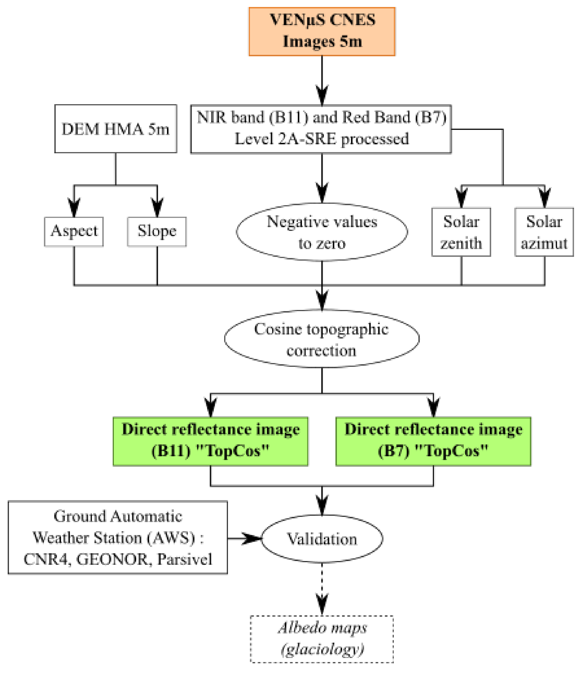
3.2.1. Slope Effect Correction

Atmospheric and radiometric slope effect corrections over mountainous areas are necessary for state-of-the-art preprocessing in optical remote sensing [53,54]. This post-processing is essential for surface albedo retrieval in rugged terrain, particularly for glaciers and snow-covered areas [55,56,57,58]. We analyze the performance of two approaches to correct the differential solar illumination effects: (1) the cosine correction taking into account only the direct illumination (lambertian case) (Figure 2) [59,60]; and (2) the Gamma correction, more complex, considering both direct and diffuse illuminations (non-Lambertian case) [18]. The Gamma process, logically more efficient for snow cover, is applied by CNES to generate the VENµS FRE product (flat reflectance) from the SRE product (surface reflectance), but is based on the coarse 90 m SRTM DEM.
Our objective here is to test whether a simple correction of direct illumination (cosine correction), if based on a higher-resolution DEM (8-m HMA DEM in this case), would be more accurate than the Gamma reflectance correction applied by CNES. In order to apply the cosine correction to the VENµS SRE product, we developed a Python script whose major steps are described below and in Figure 3.
As illustrated in Figure 2, the use of a DEM makes it possible to determine the respective illumination cos( γ ) of each specific slope applying the following formula:
cos ( γ ) = cos ( θ s ) cos ( θ n ) + sin ( θ s ) sin ( θ n ) cos ( φ s φ n ) ,
where θs and φs are the sun zenithal and azimuthal angles; θn and φn are the slope value and orientation, respectively. Equation (3) creates the illumination angle and the normalized horizontal reflectance is then calculated by Equation (4):
R h o r = R × cos θ s cos γ ,     cos γ > 0.2 No   Date   Value ,     cos γ 0.2
where R is the input pixel sloping reflectance and Rhor is the output pixel corrected as in horizontal condition. Due to the low reflectance values in shaded areas, artifacts are created. We use a threshold fixed at 0.2 as in [53], below which R h o r data are discarded, as the correlation between the ground reflectance data and the corrected reflectance of the satellite images is too low. The cosine correction can be simply applied to any reflectance band, but some low illumination angles are over-corrected [61]. The reason is that these areas receive more diffuse radiation not accounted for in the cos( γ ) direct calculation. We apply Equations (3) and (4) using the HMA DEM. Our cosine output product is then named TopCos HMA (referred to as such here-after). This model is run on the VENµS SRE product for (i) the B11 near-infrared spectral band (865 µm) concerning albedo application, because it is least impacted by atmospheric effects, and (ii) the B7 red spectral band (662 µm) for cloud and snow mapping applications (Figure 3).
Additionally, we compute a fourth reflectance product, named TopCos SRTM (Table 4), which is based on the SRE product corrected with the cosine correction using the SRTM DEM (90 m). The aim is to analyze the influence of different DEM spatial resolutions with the same radiometric correction method.

3.2.2. Reflectance Product Statistical Evaluation Strategy

A statistical comparison is conducted among the four reflectance products; thus, the contribution of the bias and STD to the RMSE is calculated for each reflectance product. Appendix A exhibit the detailed metrics results for each site. As a reminder, the root-mean-square error (RMSE) is retrieved by the bias and dispersion (STD) calculations. Their respective contribution (%) is simply given by:
Bias   contribution = 100 × Bias 2 RMSE 2 ,
and,
STD   contribution = 100 × STD 2 RMSE 2 ,
with:
RMSE 2 = Bias 2 + STD 2 ,
where RMSE is the root-mean-square error and STD is the standard deviation. The Pearson coefficient R 2 is also calculated with:
R 2 = 1 S S r e s S S t o t ,
where S S r e s is the residual sum of squares and S S t o t is the total sum of squares.
Finally, in order to highlight the best product and the best site in terms of performance, we use a normalized skill score. The transformation to a generic skill enables us to avoid the problem of having different units for the different metrics. The normalized skill score ( N S S ) for each kind of metric is calculated with:
N S S RMSE site ,   product = 1 RMSE   site ,   product max RMSE ,
where N S S RMSE represents the normalized RMSE skill score for a specific site and product, RMSE is the root-mean-square error for a specific site and product, and max RMSE is the highest RMSE among all sites and products.
N S S Bias site ,   product = 1 Bias   site ,   product max Bias ,
where N S S Bias represents the normalized bias skill score for a specific site and product, Bias is the bias absolute value for a specific site and product, and max Bias is the highest bias among all sites and products.
N S S STD site ,   product = 1 STD     site ,   product max STD ,
where N S S STD represents the normalized standard deviation skill score for a specific site and product, STD is the standard deviation for a specific site and product, and max STD is the highest STD among all sites and products.
N S S R 2 site ,   product = R 2   site ,   product max R 2 ,
where N S S R 2 represents the normalized Pearson coefficient skill score for a specific site and product, R 2 is the Pearson coefficient for a specific site and product, and max R 2 is the highest R2 among all sites and products. Once all skill scores are calculated for each value at each site, we calculate the average normalized skill score (ANSS) for each type of metric, by product and by site (ANSS by row and column). Higher values correspond to better performance.

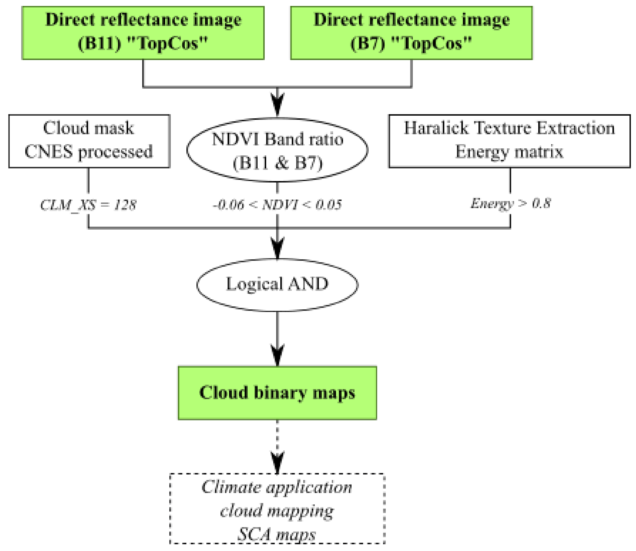
3.2.3. Cloud Mask Processing

As a reminder, in this study, our goal is not only to apply a cloud mask to the VENµS images to retrieve a satisfactory snow mapping chain, but also to use all cloudy images in the aim of mapping the cloud cover evolution over the measuring period for a climate application (monsoon regime). Based on the Hagolle algorithm [51], we observe that the CLM_XS product applied to the SRE product obscures several snow-covered areas in our study site, which are clearly visible on the Level-1C images of VENµS. This is partly due to the 2-pixel-wide dilation of the cloud mask at reduced resolution, applied to include thin clouds at the edge of thicker clouds [16]. Due to the lack of a SWIR band on the VENµS sensor, we have developed another approach dedicated to cloud mapping improvement. We aim to leverage and refine the CNES cloud masks to retrieve mor e information about the snow cover on the ground and create cloud and SCA maps databases with a 2-day frequency, at a 5 m spatial resolution. We therefore propose a complementary process based on a hybrid textural/radiometric approach in order to improve and optimize the CLM_XS product. The Python algorithm to retrieve cloud masks for VENµS is part of the VENuS_cosine_correction algorithm.
Mainly applied during the 1970s for geographical application, textural features extraction from optical data are based on mathematical morphology applied to grey-tone images. The Haralick textural decomposition is applied on co-occurrence matrices [62,63] and offers attractive results using entropy and energy as parameters. Energy indicates the angular second-moment feature (ASM), which is a measurement of local grey-level uniformity. Taking into account the textural behavior of the snow and clouds according to uniformity, the energy parameter is more appropriate for this study than entropy. Energy is defined by the following relationship:
Energy   = ASM
where:
ASM = i j p d 2 i , j
with p d i , j as (i,j)-th element of the grey-level co-occurrence matrix [63]. We also use the NDVI (Normalized-Difference Vegetation Index) between red and near-infrared bands (respectively B7 and B11) to help separate snow, ice and cloud features from other land uses. NDVI is defined as:
NDVI = R N I R R r e d R N I R + R r e d
where R N I R is the surface reflectance in the NIR (861.1 nm) spectral band and R r e d (666.2 nm) is the surface reflectance in the red spectral band.
Our cloud mask product, named CloudCov, is the intersection of masks based on the NDVI and Energy values (Table 5), and the CLM_XS product. Thresholds were determined by radiometric tests on several VENµS dates in winter, with lots of snow. The CLM_XS product is a conservative mask, which overestimates the cloud cover. This is why we intersect it ( denotes the intersection function) with the combination of NDVI and Energy, which tends to miss some cloud-covered areas. The CloudCov product is defined according to Equation (16):
CloudCov = NDVI 0.06 NDVI 0.05 CLM _ XS = 128 Energy > 0.8
Clouds over a snow-covered area that are not detected in CLM_XS are also not detected as clouds in our cloud mask.
Once the CloudCov mask has been computed for each VENµS date using TopCos HMA products (NDVI from B7 and B11), all TopCos HMA (B11 only) products (138 dates) are re-computed, this time considering the CloudCov mask. This second process enables the provision of TopCos HMA reflectance products where cloud pixels have the value 128, and thus can be easily discriminated for further applications (Figure 4 describes the complete workflow).

3.2.4. Cloud Mask Statistical Evaluation Strategy
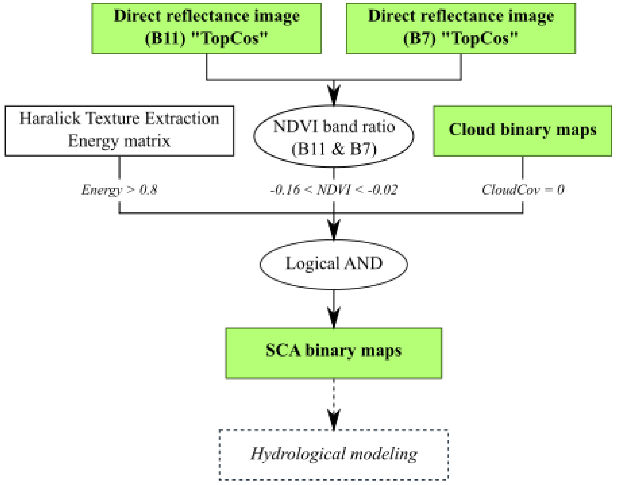
In order to assess the concordance between a control sample and the cloud mask product, we use the Kappa coefficient [64,65], equivalent to the Heidke Skill Score (HSS) [27,34,66]. By calculating the improvement in the algorithm’s behavior relative to a reference behavior such as chance, the HSS measures relative skill. This is expressed as the proportion of pixels correctly classified relative to the number of pixels correct by chance in the complete lack of skill [66]. It allows us to evaluate the classification performances of the CloudCov mask at the pixel scale. The CloudCov mask, manually corrected and improved, is considered to be the actual situation. Table 6, based on Equations (17) and (18), summarizes the metrics used to assess the CloudCov mask.
The Kappa coefficient is retrieved using:
p 0 = T P + T N T P + F P + F N + T N
and:
p e = T N + F P × T N + F N + F N + T P × T P + F P ( T P + F P + F N + T N ) 4
where p 0 is the observed proportionate agreement, p e is the overall random agreement probability, TN is the true negative pixels; TP is the true positive pixels; FN is the false negative pixels and FP is the false positive pixels. TN means the algorithm correctly predicted that the pixel has no cloud. TP means the algorithm correctly predicted that the pixel has clouds.

3.2.5. SCA Outputs

The SCA product is generated using the TopCos and CloudCov chains. Following a similar reasoning to the CloudCov mask, snow pixels are extracted by calculating the following intersection (Equation (19)). Note that a CloudCov value of 0 means no cloud.
Snow   pixels = NDVI 0.16 NDVI 0.02 CloudCov = 0 Energy > 0.8
If these conditions are fulfilled, a snow pixel will get the value 1. Then we code cloud pixels with the value 128 (using the CloudCov mask computed formerly) and other land uses with a value of 0. Figure 5 describes the SCA product workflow and example of maps are given in Figure A1. Under cloudy conditions, our classification algorithm clearly distinguishes snow from clouds. Note that bare ice areas of glaciers are not classified as “snow”, while accumulation areas are. Snow-covered lakes are included, and if not snow-covered, are classified as 0 (other land use).

4. Results

4.1. Producing Reflectance Maps from VENµS Images as a Proxy of Albedo Maps

4.1.1. Comparison of TopCos Products (HMA, SRTM) and CNES Products (SRE, FRE)

To compare those four products, we select a subset (Figure 1) in the NE part of the VENµS tile, representative of fully snow-covered areas without cloud coverage (Figure A2). Figure 6 presents the frequency of reflectance occurrences for SRE, FRE and the two TopCos products, HMA and SRTM. Note that for Figure 6, normalization of all data was performed using Equation (20):
z i = x i min x max x min x ,
where z i is the ith normalized data and x = x 1 ,   ,   x n is the reflectance for each pixel.
The plots in Figure 6 are representative of the general pattern observed in the complete database. On the one hand, for SRE and FRE products, over the entire range of values, the frequency of occurrence of each reflectance value is homogeneous. On the other hand, TopCos products (HMA and SRTM) indicate reflectance values with a peak around 0.25 (Figure 6). As a reminder, when charting the normalized reflectance occurrence frequency, peak values are left-shifted, to fit the 0–1 interval. Low reflectance values with limited dispersion mean that the image has limited radiometric contrast. The TopCos products have less contrasts than the SRE and FRE. In TopCos, there is indeed a reduction in the difference between illuminated and shaded areas induced by the cosine correction [67].
Figure 7 shows the probability density of the reflectances for the four reflectance products on the same subset as Figure 6. All products have their mode close to 1, characteristic of the snow response. On the one hand, SRE and FRE reflectances are constrained to 1.3 due to a LUTs (Look Up Tables) limit in the atmospheric correction process of VENµS images. On the other hand, the cosine method is known for its overcorrection effect, especially on less illuminated regions: the lower the value of cos( γ ), the higher the overcorrection [53]. This phenomenon may be accentuated by the darker pixels in neighboring shadow areas (no correction applies since cos( γ ) is negative or zero) [59]. Here, the cosine method is applied only for cos γ > 0.2 ( γ < 78 ° ) to avoid artifacts. The larger reflectance amplitude observed for TopCos products is logically induced by the cosine correction, whereas FRE computed via the Gamma method (direct and diffuse illumination) is closer to broad band albedo from ground data. It should be noted that the fine HMA DEM (5 m) reduces this overcorrection in regard to the larger SRTM one (90 m), suggesting that a finer DEM enables better consideration of local topography, and thus more realistic reflectances.

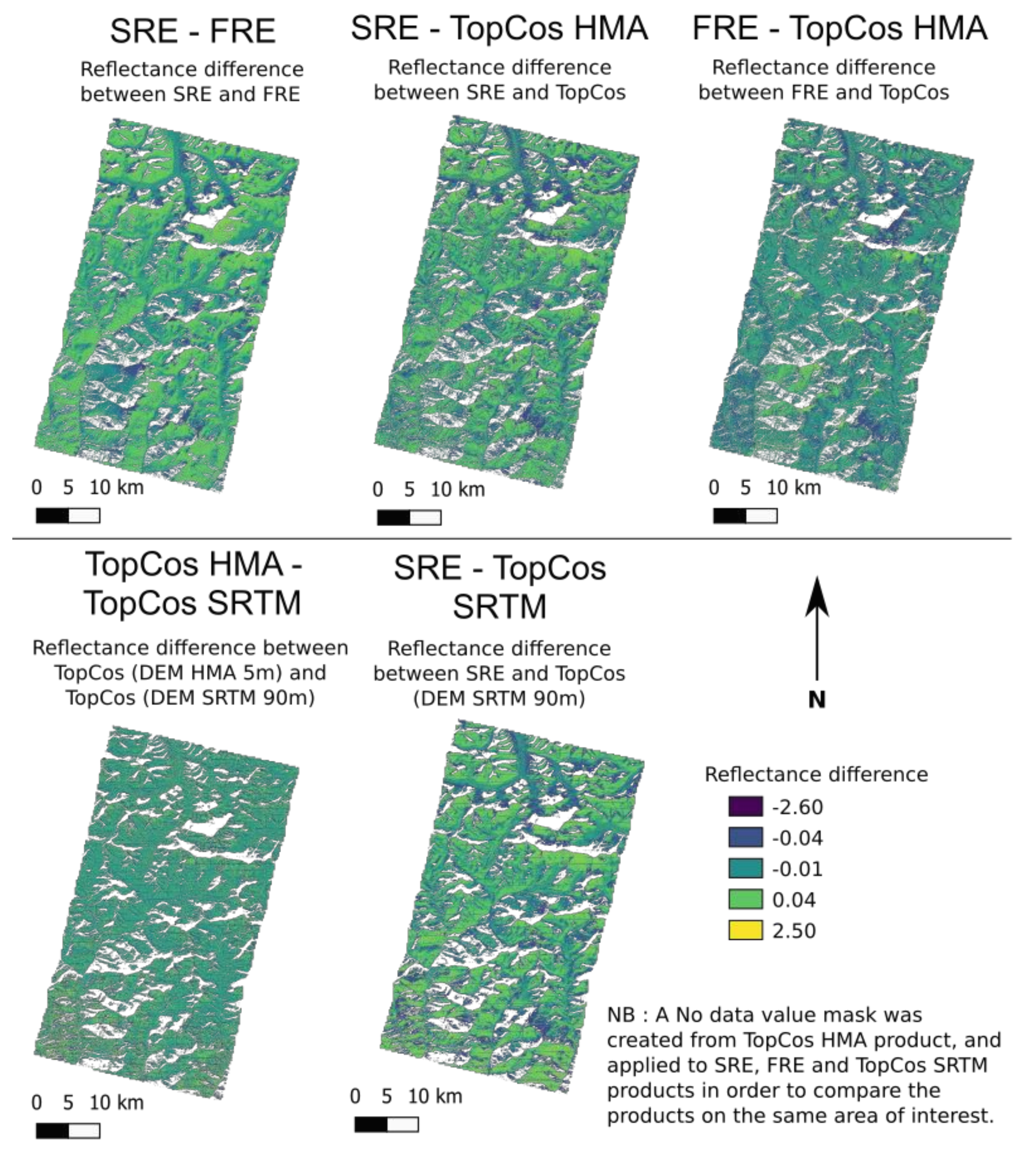
4.1.2. Difference between the Four Reflectance Products

In order to understand the high-resolution DEM influence on the radiometric correction, we analyzed the differences between the various reflectance products (Figure A3). The analysis is carried out here on the 7 December 2017 VENµS image, with no cloud and average snow cover extent. As a reminder, a summary of all the products computed is available in Table 4. Comparison between the two CNES products (SRE and FRE) shows that surfaces with steep slopes exposed to the sun are corrected negatively, with the reflectance of these areas decreasing when the gamma correction is applied. In contrast, flat areas less exposed to the sun are corrected positively (i.e., reflectance increases in the FRE product). The difference between the SRE and TopCos HMA indicates that the DEM resolution increases the level of detail and thus the TopCos HMA product should be preferred. Comparison between the two corrected products FRE and TopCos HMA reveals that the TopCos HMA product further reduces the high reflectance values in sun-exposed areas.
Finally, to analyze only the influence of DEM resolution, we compare the two TopCos products (HMA and SRTM); the difference between them shows the same mean bias correction all over the tile (around 0.01 difference in their mean values). Use of an initial DEM with an 8 m resolution, close to the VENµS spatial resolution (5-m) offers a sharp relief description and more variation in the reflectance within a neighborhood which is a benefit in snow detection.

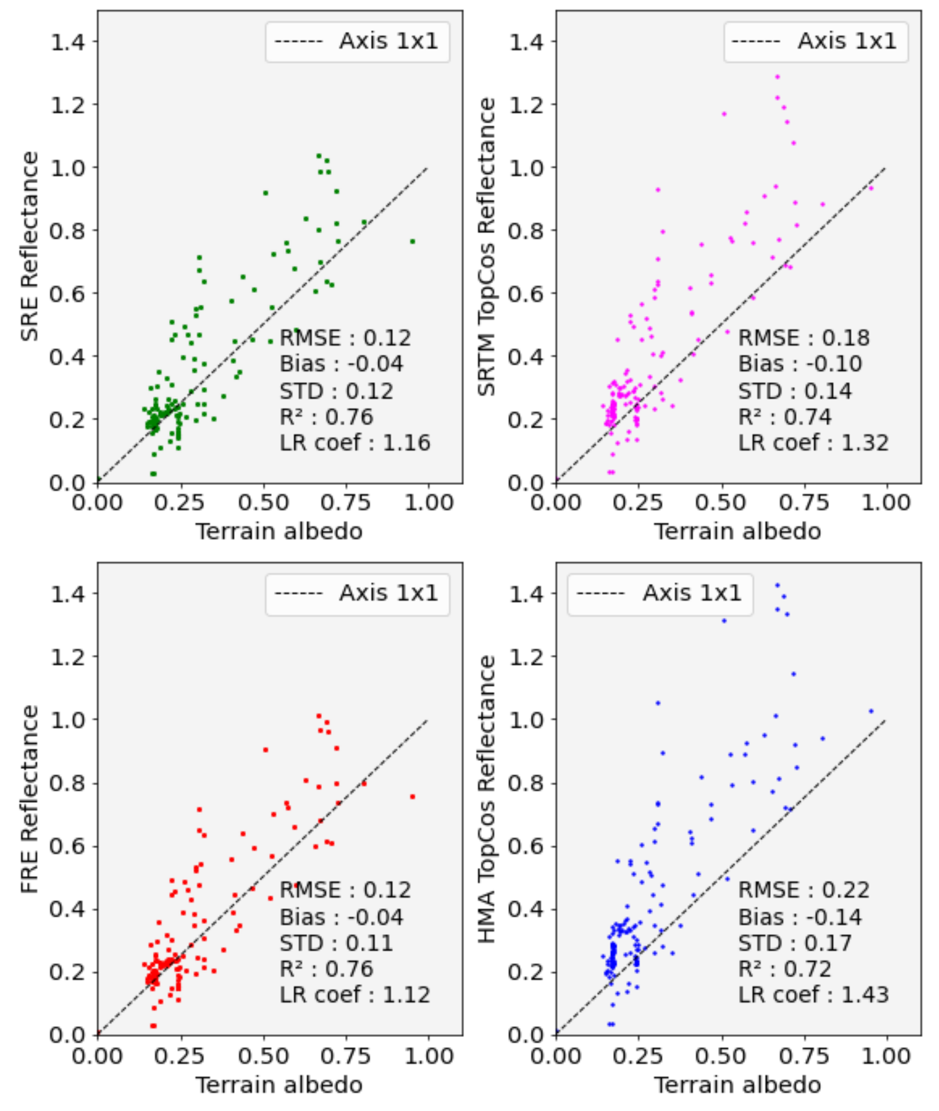
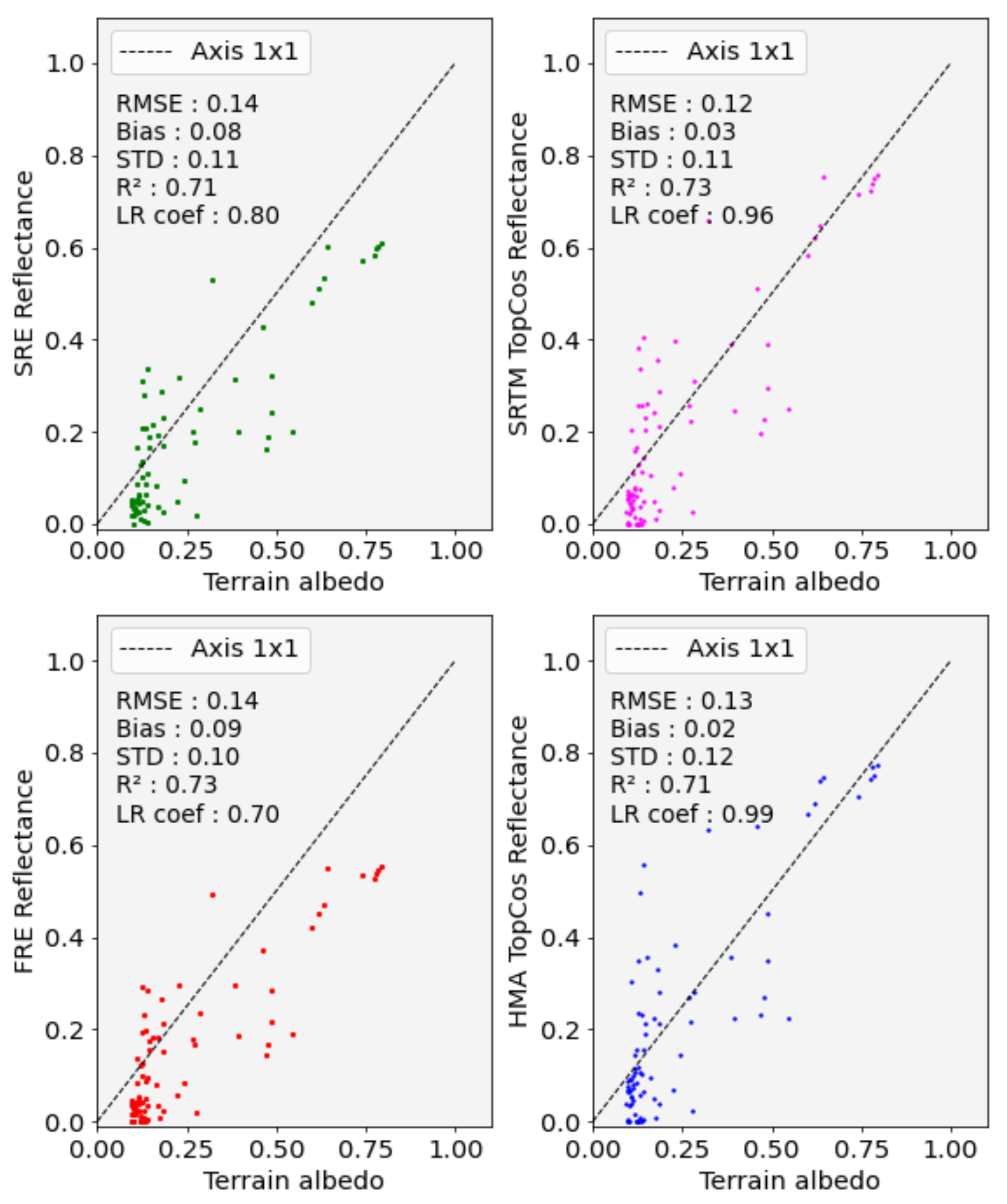
4.1.3. Comparison of TopCos and CNES Products with Shortwave Albedo Measurements

  • Temporal evolution
Here we compare satellite data registered in a spectral band of near-infrared (B11, 865 µm), with a narrow bandwidth of 40 µm, with broadband albedo sensors on the ground (0.305 < λ < 2.8 µm) for incident and reflected short-wave radiation. Although not a like-for-like comparison, we pursue this comparison to explore the possibility of using the remotely sensed data to infer broadband albedo relevant for the surface energy balance. Figure 8 illustrates the results for the three ground measurement sites. It is important to note that during the monsoon (JJAS), Pyramid site is not covered with snow due to its lower elevation (5 035 m a.s.l.), leading to low reflectance values. Apart from the monsoon, the four reflectance products follow the ground albedo pattern with each instance of snowfall characterized by a sharp albedo increase, followed by a decay. At Pyramid (Figure 8a), when there is snow on the ground, TopCos HMA and FRE products are both closer to the terrain albedo values, whereas the SRE and TopCos SRTM products are respectively impacted by (i) the lack of slope radiometric correction, and (ii) the low DEM resolution effect. Changri Nup site (Figure 8b) is regularly covered by snow in winter (DJF), and unlike Pyramid site, is consistent with more frequent high reflectance values. During the monsoon, there is no snow on the ground, the reflectance values are low and similar to the ground albedo values as for the Pyramid site. When snowfall occurs in the winter period, the four reflectance images follow the temporal variability of the in situ albedo values; the reflectance increases, then slowly decreases (gradual melting of the snow), and the four products offer a similar response considering alternatively each pair of products as for Pyramid site. At South Col site (Figure 8c) we can observe several high reflectance values during the monsoon, suggesting significant snow cover, induced by solid precipitation at such elevation (7945 m a.s.l.).
The three sites of this study have distinct seasonal behavior due to their specific locations and surface states (Table 2), but similar temporal variabilities occur between the four reflectance products and ground measurements: (i) when there is little or no snow on the ground, all four reflectance products exhibit low reflectances close to the in situ albedo measurements. The three corrected products (FRE, TopCos HMA and TopCos SRTM) are close to each other; (ii) during snowfalls the four products follow the ground albedo rise. More precisely, TopCos products (HMA and SRTM) are closer to the terrain albedo when the site is snow-covered while CNES products (SRE and FRE) tend to underestimate the in situ albedo values. The raw SRE products are the furthest from the observations.
  • Statistical comparison
Table 7 offers a synthesis of all metrics for the four reflectance products compared to albedo measured in situ. The details of the normalized skill scores used to calculate the ANSS are described in Table A1. We can observe that, globally, all metrics offer satisfactory results. In particular, we can see that (i) for the FRE product, RMSE values are low on the three sites, and (ii) from the three corrected products (FRE, TopCos HMA and TopCos SRTM), the FRE product has the best mean RMSE on the three sites. The dispersion is always the most impactful on the RMSE. Using the average normalized skill score (ANSS) reveals that the best product according to statistical performances is the FRE from CNES, and the site for which this is most effective is Pyramid (Figure A4). However, since Pyramid site is rarely snow-covered, observing the correlation between reflectance products and in situ albedo is more difficult than the two other sites. Changri Nup (Figure A5) is the site with the lowest performance but it has more temporal variability. On the one hand, the CNES FRE and SRE products are similar and FRE introduces great metrics (STD contributing to the RMSE for 84% while the bias contributes only for 11%). On the other hand, the TopCos HMA has a dispersion and bias that similarly impact the RMSE (60% and 40% respectively) and TopCos products present significant biases (around 0.1). South Col site (Figure A6) is the second-best site of application according to Table 7. The two CNES products are similar, likewise at the Changri Nup site. The FRE product offers great metrics; however, its RMSE is larger than TopCos products (dispersion and bias contribute equally to the RMSE of the FRE product, respectively 51% and 41%). TopCos HMA product shows a low RMSE and the lowest bias, so it would therefore be less affected by overcorrection effects (dispersion and bias contributions to RMSE are 100% and 2% respectively). We can observe that Pyramid and South Col sites have limited temporal variability, with respectively little or much snow cover throughout the year, which impacts the statistical results.

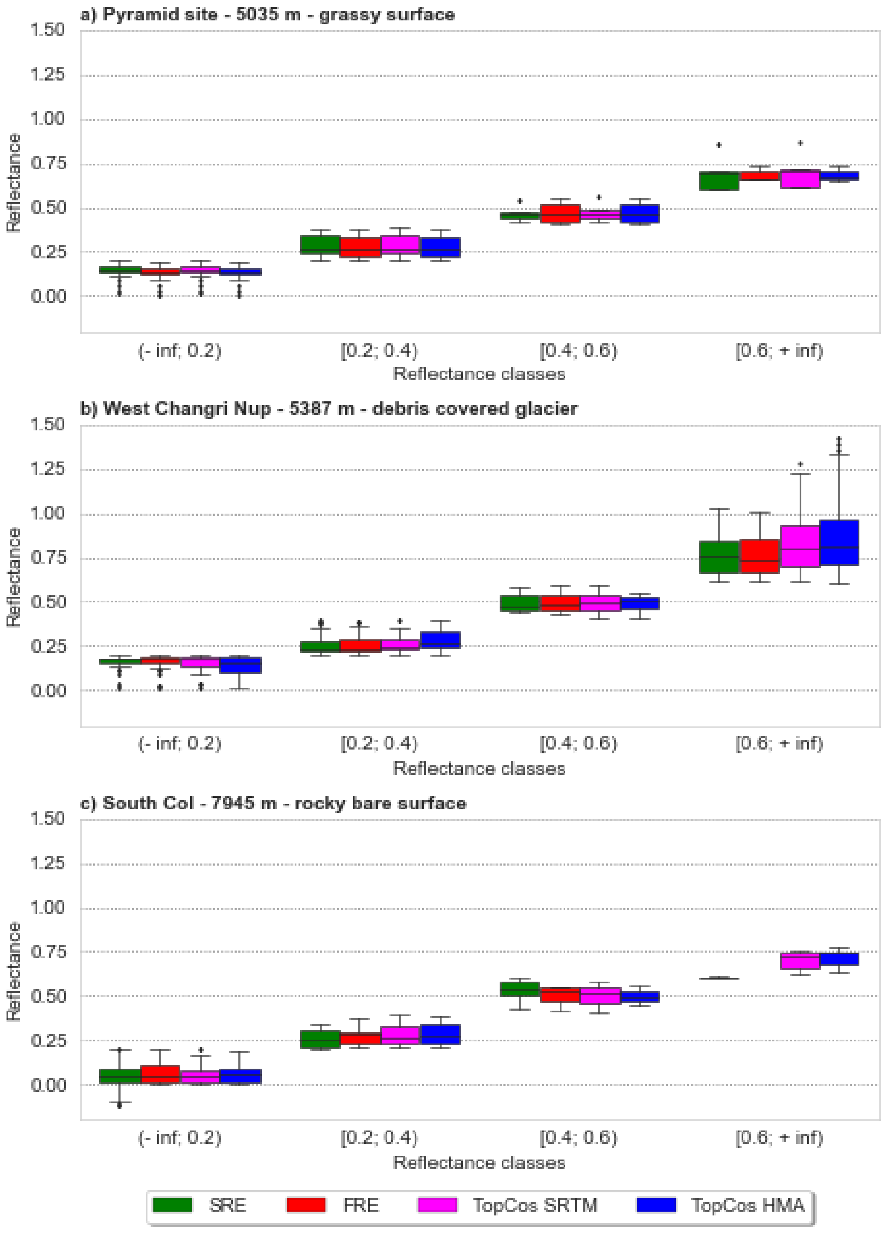
4.1.4. Distribution of Reflectance Values according to the Correction Used

By presenting the reflectance values under classes, an analysis of the reflectance distribution according to each reflectance product, and thus according to the correction method, can be performed (Figure 9). Pyramid site (low snow cover) (Figure 9a) reveals a similar behavior for the four reflectance products in low reflectances (<0.4). Above 0.4, SRE and TopCos SRTM products follow the same trend, as does the FRE-TopCos HMA pair. For reflectance higher than 0.6, Figure 9a suggests that the cosine correction algorithm used to compute TopCos HMA has the same effect as the MAJA Gamma algorithm (CNES). However, most reflectance values are below 0.7, which means Pyramid site is rarely covered by snow. Results on the Changri Nup site (more often snow-covered) (Figure 9b) indicate that for reflectances below 0.6, all the studied products are very similar to each other. However, for higher reflectances, two product pairs can be distinguished: the TopCos products show analogous behavior between each other, as do CNES products. At South Col site (Figure 9c) the behavior of all the products remains the same for low reflectances (<0.6). Above this threshold, the same two pairings as in the Changri Nup site are observed.

4.2. Cloud Mapping

4.2.1. Statistical Analysis of the CloudCov Product

Our algorithm developed to retrieve cloud cover is presented in Section 3.2.3. (Table 5 and Figure 4) and an example is presented in Figure 10. The cloud mask produced is named CloudCov. Our approach enables significant optimization of the CNES cloud mask CLM_XS (Figure 10b). A representative example (8 August 2018), describing more precisely the cloud outlines versus snow-covered and non-snow-covered areas on the ground, is presented in Figure 10c. On average, the CLM_XS mask classifies 27% of the pixel as clouds, while CloudCov classifies only 12% as clouds on the same images. This is a significant gain in usable imagery. However, as the CloudCov product extends near the edge of the clouds, it also contains fewer cloud-cast shadows (Figure 10). Depending on the objective, one can still favor the CLM_XS mask as it is more conservative.
The CloudCov product estimated from our algorithm is then manually corrected (manual delineation) and used as a reference in the confusion matrix (Figure 11), computed on the 238 VENµS dates, to quantify the gain obtained with the CloudCov mask. Our cloud mask contains 96% well-classified pixels, while CLM_XS cloud mask only has 81% (Figure 11 and Table 8). Thus, the CloudCov mask is 15% more accurate than CLM_XS mask, but the precision improvement is even more significant, with a 35% gain compared to the CLM_XS mask.
We compare both the CNES CLM mask and the CloudCov mask retrieved from our algorithm to the actual situation. Table 8 summarizes the results for the CNES CLM_XS mask and the CloudCov mask pixel study. While the CLM_XS mask has an HSS score under 50%, the CloudCov mask computed by our algorithm seems to perform very well with a Kappa score above 80%.

4.2.2. Temporal Analysis

Figure 12 shows the synthesis of the CloudCov masks computed over the complete VENµS acquisition period and seasonally aggregated. This figure enables the monitoring of cloud behavior through the different seasons of the year. Post-monsoon and winter are the least cloudy seasons, with a mean cloud occurrence of 10%, while monsoon is the cloudiest one with a mean occurrence of 40% (note that the monsoon cloud occurrence is likely underestimated, as fully cloud covered images are not available—118 VENµS images were discarded).

4.3. Snow Cover Area Mapping

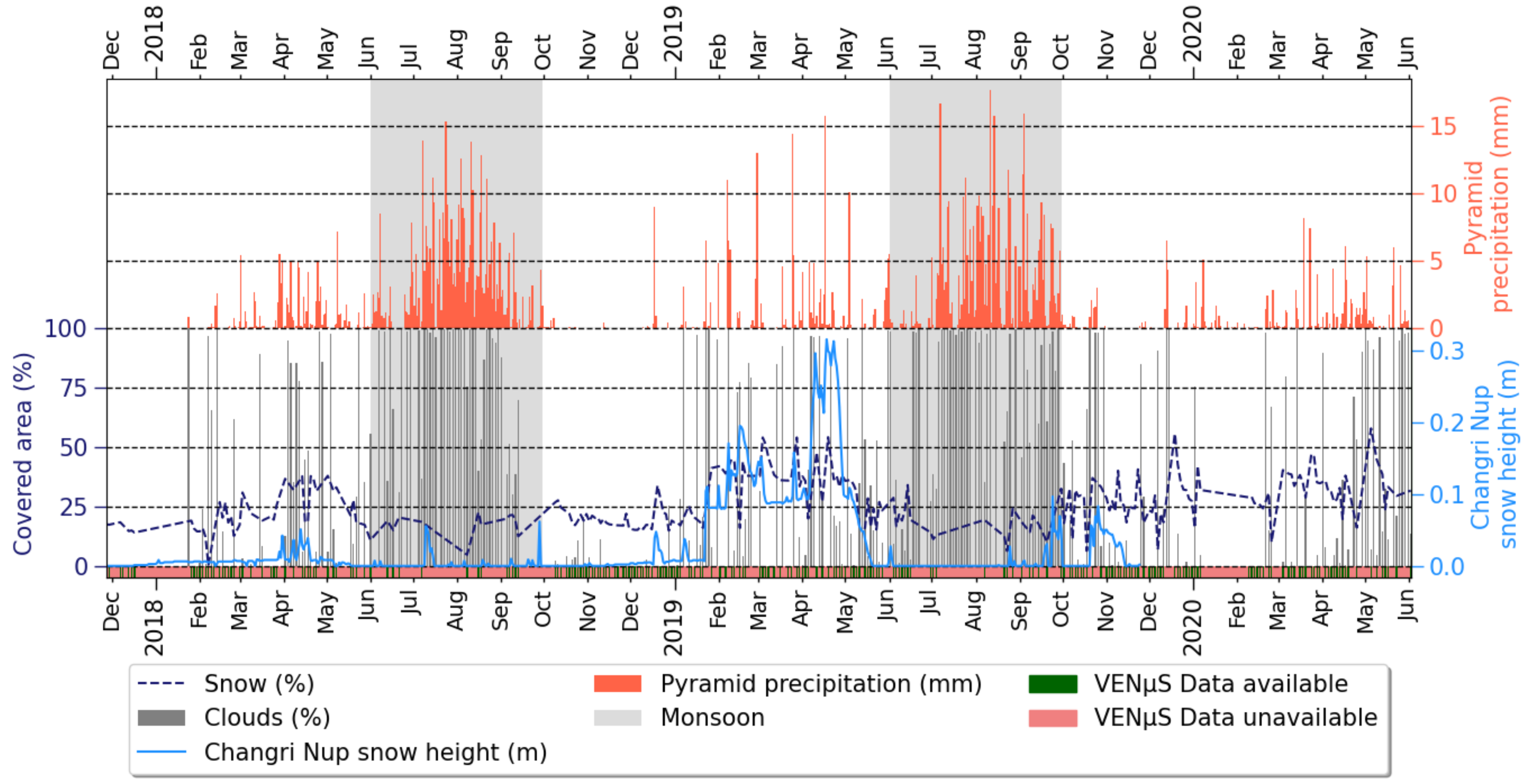
4.3.1. Comparison of Snow Cover with Meteorological Data

For unavailable VENµS data due to high cloud cover, we selected the MAJA chain cloud percentage and filled the cloud cover percentage database retrieved from available images. We compared ground data versus estimations of the extent of snow and cloud covers in Pheriche basin from VENµS images, in order to verify their consistency (Figure 13). We consider here the complete VENµS time period database (November 2018 to June 2020). Figure 13 (top) shows the precipitation at Pyramid site. Outside the rainy season, high cloud cover events are observed intermittently. During the monsoon, periods of high cloud cover persist for several days, whereas outside the rainy season they are more short-lived (Figure 13, bottom). Looking at Pyramid site’s precipitation, two phenomena are apparent: (i) the high frequency of pre-monsoon precipitation coincides with the snow height in this period (and so with the cloud cover percentage increase), and (ii) the even greater precipitation frequency during the monsoon. However, the link between cloud cover and precipitation is not obvious and heavy cloud cover does not mean heavy precipitation, or precipitation at all. In addition, the analysis is partial, due to the unavailability of images during the monsoon (high cloud cover percentage), which induce a lack of information on the extent of snow cover. The comparison between cloud cover, snow cover and snow height does not show an obvious link (Figure 13, bottom). Some increases in snow height are related to high cloud cover, but not systematically. Surface snow cover is more persistent in the winter months, with coverage then increasing in the Feb–May pre-monsoon period, before accelerating and then declining during the monsoon. Note that this decline may be an artefact from the strong cloudiness in the monsoon, which prevents detection of the snow cover on the ground. As expected, at Changri Nup site, the snow is higher in the winter season and before the monsoon; the Pheriche basin snow cover percentage follows the same pattern. By joining those data, it seems that for the Pheriche watershed, there is a decrease in the extent of snow cover at the beginning of the monsoon, but likely an increase in the thickness of the snow cover at elevations higher than the glacier equilibrium line, i.e., approx. 5500 m a.s.l.

4.3.2. Seasonal Evolution of SCA versus Cloud Cover at the Watershed Scale

With snow cover area maps (SCA) retrieval, a comparison between the two watersheds of Dingboche and Pheriche is conducted. An example of VENµS SCA maps is presented in Figure A1. For each basin, Figure 14 presents the percentage of the surface area covered by snow or clouds. Although VENµS images with high cloud cover are not available online, the cloud cover percentage has been set to 100% for dates where the CNES’ MAJA chain detects 100% cloudiness. The two watersheds offer a similar pattern, coherent with the season. In post monsoon and winter from October to February, there are few clouds and snow coverage is quite constant. In 2018 and 2019, during the pre-monsoon, from April to May, the snow cover progressively decreases and the cloud cover increases. Then, in the monsoon, from June to September, there is little snow cover detected because of the high cloud cover and of the lack of available VENµS images during massive cloud cover episodes.

5. Discussion

5.1. TopCos HMA Product

As a reminder, we compare in situ albedo measurements (broad band albedo, 0.305-2.8 µm) to narrow reflectance observations (0.865 µm). Overall, none of the reflectance products stands out as an ideal proxy for albedo when compared with field measurements. While all the reflectance products follow the right temporal evolution of albedo, they appear to have biases and performances that are site dependent. This means that empirical calibration is required before using FRE or TopCos HMA reflectances as albedo proxies for applications, such as snow and ice surface energy balance computation. The FRE product seems to be the best product among all sites (Table 7); however, the TopCos HMA product has a better NSS for the Pyramid and South Col sites than for the Changri Nup site (Table A1). Additional reflectance bands in long-wave infrared are required to calculate albedo [68]. The lack of such measurements from the VENµS plateform is a limitation in snow and glaciological applications for energy balance. However, both FRE and TopCos HMA products have satisfactory results with a low RMSE, especially at South Col site: 0.14 for the FRE product and 0.13 for the TopCos HMA product. They show great potential in differentiating snow from rock or bare ice.
Figure 9 highlights the overcorrection in the TopCos HMA reflectance image. A threshold of 0.2 is set on the cos( γ ), equivalent to a maximum illumination angle of 78.5°, whereas in Teillet et al. [59], a threshold of 55° is recommended. We made this choice to retain sufficient data, knowing some artifacts and overcorrection could appear. Indeed, an illumination angle close to 90° leads to a high dividing factor and thus to an overcorrection.
Looking at the statistical analysis, the high-resolution HMA DEM does not yield better results than the FRE product corrected with SRTM. In [67], radiometric slope correction using coarse spatial resolution of SRTM offers slightly better results than using fine spatial-resolution DEM from an optical sensor, due to the better vertical accuracy in SRTM retrieved from the active radar (SAR) mode. This means that the cosine correction is likely not the most efficient correction in the rough terrain of the study area. The MAJA processing chains that calculate indirect and ambient reflection (Gamma correction) seem to be better suited (FRE), despite being applied on a lower resolution DEM. It would be worthwhile to test the MAJA chain using HMA DEM as input DEM.

5.2. CloudCov Product

Different methods exist in the literature for cloud detection processes and a recent and complete review is given by Nepal et al. [69]. Cloud detection in remote sensing, based on deep learning and machine learning using dense neural networks, actually represents a way of interest to detect clouds (clustering) with better accuracy than existing mask generation methods, i.e., threshold-based methods [70,71]. However, these algorithms need strong calculation architecture that we could not apply for this brief project. This is the reason why we proposed a simple scheme based on a hybrid method which combines co-occurrence textural matrices and radiometric parameters to improve the CLM_XS mask. Another advantage of the CloudCov product is that it enables working at the VENµS ground resolution, since we used a pixel-wise study. Moreover, to our current knowledge, no other study has used VENµS or any other satellite sensor with high spatial and temporal resolution to monitor the spatio-temporal evolution of cloud cover.
In Figure 12, a striking topographic effect is observed in post-monsoon, winter and pre-monsoon at the level of the Mount Everest (Figure 12a,b). Westerly winds blow the snow, creating a snow plume and an orographic banner cloud on the leeward eastern side of Everest’s summit, above the Kangshung glacier [72]. During the pre-monsoon, the early stages of the monsoon can be observed with clouds coming from South to North in the low-elevation valleys, and the Everest plume emphasizes this. Cloud intrusions from the South, in the pre-monsoon and monsoon, are constrained to elevation below 5000 m a.s.l. In the pre-monsoon and monsoon, the Tibetan plateau on the leeward side is less impacted by clouds. As a reminder, the quality and reliability of those maps is related to the amount of VENµS images available through the seasons. Note, however, that most of the monsoon images are not available for analysis here because of the impact of cloud cover (24 images not acquired for technical reason and 65 images discarded in 2018 and 2019 monsoons). To enhance the CloudCov product, an altitudinal threshold could be added in the process for the mapping of low clouds. The step of combining with solar angle could give us the cloud shadow projection on the ground. Thus, cloud shadows would be integrated into the CloudCov product. In addition, we could experiment with this method on the 6th bit of the CLM_XS mask to try to detect thin clouds.

5.3. SCA Maps

Many applications using optical remote sensing to retrieve SCA maps in Himalayas are proposed in the literature [73,74,75], particularly for this Nepalese region using MODIS images [5,14]. The GR4J [73] or the J2000 [75] hydrological models could be improved by using the SCA 5 m maps retrieved from the VENµS dataset thanks to their high spatial resolution. Indeed, the great asset of this SCA database retrieved from VENµS images relies on the high spatial (5 m) and temporal (2-day) resolution of this sensor. These SCA maps will be dedicated to the validation of the snow module from a distributed hydrological model DHSVM-GDM currently applied at IGE [5,13], and actually only based on a daily MODIS 500 m images dataset. The very high temporal resolution of the VENµS satellite is an asset, especially in monsoon conditions, even if there are clouds. Furthermore, such a database is of interest to the community studying the hydro-glaciological context of the region.
In the recent study from Baba & Gascoin [34], an unsupervised classification method has been performed and compared to a supervised classification method to detect snow in VENµS images, showing that a supervised classification gives better results. Since one of the main limitations of this approach is the cloud detection (due to the absence of SWIR band on VENµS sensor) our CloudCov mask, with a 5 m resolution, could be applied ahead of the classification. Then, their method could be tested on this new product, to better discriminate clouds from snow and improve the computed SCA maps.

6. Conclusions

The aim of this study was to evaluate and quantify the performance of different products retrieved by the CNES processing of the VENµS database over the Everest region in Nepal for glaciological and hydro-climatic applications. In such a high-mountain context, the focus was set on the interest in adding a fine DEM to the processing chain to enhance the pre-existing quality of the high temporal and spatial resolution from remote data provided by the VENµS sensor. The major findings are the following:
(i)
No consistent benefits for assessing the spatio-temporal evolution of surface albedo are retrieved using a cosine radiometric correction enhanced by a fine 5 m DEM regarding the Gamma one carried out with 90 m SRTM by CNES. The CNES FRE product offers efficient results versus in situ measurements for albedo retrieval, because Gamma correction takes into account both direct and diffuse illumination contributions. The cosine correction based only on the direct illumination can induce higher values versus broad band albedo from ground data, even using a precise DEM intended to better reduce the radiometric slope effects.
(ii)
We obtained a significant improvement with the TopCos product as an enhancement for cloud cover mapping and satisfactory results for seasonal snow mapping. Our novelty is to compute a hybrid product by merging a radiometric index (NDVI) and a textural approach (Haralick energy matrix) to overtake the CNES initial cloud mask performance.
(iii)
Furthermore, SCA maps are also improved since they are obtained using the CloudCov mask.
It appears that no other study using VENµS or any Very High Resolution (VHR) sensor dedicated to monitoring the spatio-temporal evolution of cloud cover has been conducted. Using images usually discarded because of cloudiness to study the spatio-temporal evolution of clouds in this region could be of interest, in particular to track cloud cover over the year. In conclusion, the recommendation (for users of future VENµS missions) is to apply a Gamma pre-processing chain with fine DEM at the same sensor resolution (i.e., 5 m for VENµS) and a mixed spectral-textural approach on the CNES cloud mask to improve the cloud masking/tracking in high mountain environments, including snow and glacial areas.

Author Contributions

Conceptualization, J.-P.D. and Y.A.; Methodology, Z.B., J.-P.D. and Y.A.; Software, Z.B.; Validation and Formal Analysis; Z.B., J.-P.D., P.W., Y.A., F.B. and M.E.; Data Curation, Z.B., P.W., M.E., B.P. and T.M.; Writing-Original Draft preparation, Z.B. and J.-P.D.; Writing-Review & Editing, P.W., F.B., Y.A., M.E., B.P. and T.M.; Supervision, J.-P.D.; Project administration P. W. All authors have read and agreed to the published version of the manuscript.

Funding

This work has been funded and supported by the French Service of Observation GLACIOCLIM, now called CRYOBS-CLIM, part of IR OZCAR, and by the French National Research Agency (ANR) through the PRESHINE project, Grant Number ANR-13-SENV-0005.

Institutional Review Board Statement

Not applicable.

Informed Consent Statement

Not applicable.

Data Availability Statement

All data collected, pre-processed, processed, or analyzed during this study are included in this work and algorithm codes are available on GitHub at [76].

Acknowledgments

This research was part of the selected “Pointing” project from the CNES-ISA VENµS Program, thanks to CNES for the VENµS images collection (KHUMBU site). The authors are grateful to G. Dedieu and O. Hagolle from CESBIO-CNES for their support and advice, S. Pelou from CNES for technical imaging help. Thanks to L. Davaze (IGE) for his help concerning the cosine correction processing and to S. Gascoin (CESBIO-CNES) for the HMA DEM providing. The in situ measurements at Changri Nup and Pyramid sites have been supported by the JEAI HIMALICE Program (PIs: D. Shrestha, and Y. Arnaud), within the framework of the Ev-K2-CNR Project in collaboration with the Nepal Academy of Science and Technology and Tribhuvan University. We are deeply grateful to the National Geographic Society concerning fieldwork measurements at the South Col site: the albedo data collection was conducted in partnership with the National Geographic Society, Rolex, and Tribhuvan University, with approval from all relevant agencies of the Government of Nepal. Special thanks to Aurora Elmore from the National Geographic Society for her review and advice.

Conflicts of Interest

The authors declare no conflict of interest.

Appendix A

Figure A1. Snow-covered area (SCA) mapping for Pheriche and Dingboche watersheds. Example of VENµS image of 2 March 2019.
Remotesensing 14 01098 g0a1
Figure A2. Subset of the SRE product on which the TopCos no data mask is applied. Blue pixels signify no data due to the cos γ threshold. VENµS image of 27 March 2018.
Remotesensing 14 01098 g0a2
Figure A3. Mapping comparison of radiometric differences between the four reflectance products. No data values are in white.
Remotesensing 14 01098 g0a3
Table A1. Normalized skill scores (NSS) between SRE, FRE, TopCos HMA, and TopCos SRTM products and in situ albedo AWS data for the three studied sites.
SiteMetricsSREFRETopCos HMATopCos SRTM
PyramidNSS RMSE0.550.640.640.50
NSS Bias0.640.790.790.64
NSS STD0.470.530.530.47
NSS R²0.950.930.930.95
Changri NupNSS RMSE0.450.450.000.18
NSS Bias0.710.710.000.29
NSS STD0.290.350.000.18
NSS R²1.001.000.960.97
South ColNSS RMSE0.360.360.410.45
NSS Bias0.430.360.860.71
NSS STD0.350.410.240.35
NSS R²0.930.960.930.96
Figure A4. Comparison between daily field-measured albedo at Pyramid site and four reflectance products (85 days). Top: SRE vs. TopCos SRTM. Bottom: FRE vs. TopCos HMA.
Remotesensing 14 01098 g0a4
Figure A5. Comparison between daily field-measured albedo at Changri Nup site and four reflectance products (155 days). Top: SRE vs. TopCos SRTM. Bottom: FRE vs. TopCos HMA.
Remotesensing 14 01098 g0a5
Figure A6. Comparison between daily field-measured albedo at South Col site and four reflectance products (84 days). Top: SRE vs. TopCos SRTM. Bottom: FRE vs. TopCos HMA.
Remotesensing 14 01098 g0a6

References

  1. Immerzeel, W.W.; Lutz, A.F.; Andrade, M.; Bahl, A.; Biemans, H.; Bolch, T.; Hyde, S.; Brumby, S.; Davies, B.J.; Elmore, A.C.; et al. Importance and vulnerability of the world’s water towers. Nature 2020, 577, 364–369. [Google Scholar] [CrossRef] [PubMed]
  2. Azam, M.F.; Kargel, J.S.; Shea, J.M.; Nepal, S.; Haritashya, U.K.; Srivastava, S.; Maussion, F.; Qazi, N.; Chevallier, P.; Dimri, A.P.; et al. Glaciohydrology of the Himalaya-Karakoram. Science 2021, 373, eabf3668. [Google Scholar] [CrossRef] [PubMed]
  3. Pritchard, H.D. Asia’s shrinking glaciers protect large populations from drought stress. Nature 2019, 569, 649–654. [Google Scholar] [CrossRef]
  4. Savéan, M.; Delclaux, F.; Chevallier, P.; Wagnon, P.; Gonga-Saholiariliva, N.; Sharma, R.; Neppel, L.; Arnaud, Y. Water budget on the Dudh Koshi River (Nepal): Uncertainties on precipitation. J. Hydrol. 2015, 531, 850–862. [Google Scholar] [CrossRef]
  5. Mimeau, L.; Esteves, M.; Zin, I.; Jacobi, H.W.; Brun, F.; Wagnon, P.; Koirala, D.; Arnaud, Y. Quantification of different flow components in a high-altitude glacierized catchment (Dudh Koshi, Himalaya): Some cryospheric-related issues. Hydrol. Earth Syst. Sci. 2019, 23, 3969–3996. [Google Scholar] [CrossRef] [Green Version]
  6. Matthews, T.; Perry, L.B.; Koch, I.; Aryal, D.; Khadka, A.; Shrestha, D.; Abernathy, K.; Elmore, A.C.; Seimon, A.; Tait, A.; et al. Going to Extremes: Installing the World’s Highest Weather Stations on Mount Everest. Bull. Am. Meteorol. Soc. 2020, 101, E1870–E1890. [Google Scholar] [CrossRef]
  7. Hersbach, H.; Bell, B.; Berrisford, P.; Hirahara, S.; Horányi, A.; Muñoz-Sabater, J.; Nicolas, J.; Peubey, C.; Radu, R.; Schepers, D.; et al. The ERA5 global reanalysis. Q. J. R. Meteorol. Soc. 2020, 146, 1999–2049. [Google Scholar] [CrossRef]
  8. Maussion, F.; Scherer, D.; Mölg, T.; Collier, E.; Curio, J.; Finkelnburg, R. Precipitation seasonality and variability over the Tibetan Plateau as resolved by the high Asia reanalysis. J. Clim. 2014, 27, 1910–1927. [Google Scholar] [CrossRef] [Green Version]
  9. Bolch, T.; Shea, J.M.; Liu, S.; Azam, F.M.; Gao, Y.; Gruber, S.; Immerzeel, W.W.; Kulkarni, A.; Li, H.; Tahir, A.A.; et al. Status and Change of the Cryosphere in the Extended Hindu Kush Himalaya Region. In The Hindu Kush Himalaya Assessment; Wester, P., Mishra, A., Mukherji, A., Shrestha, A., Eds.; Springer International Publishing: Cham, Switzerland, 2019; pp. 209–255. [Google Scholar]
  10. Viviroli, D.; Archer, D.R.; Buytaert, W.; Fowler, H.J.; Greenwood, G.B.; Hamlet, A.F.; Huang, Y.; Koboltschnig, G.; Litaor, M.I.; López-Moreno, J.I.; et al. Climate change and mountain water resources: Overview and recommendations for research, management and policy. Hydrol. Earth Syst. Sci. 2011, 15, 471–504. [Google Scholar] [CrossRef] [Green Version]
  11. Gascoin, S.; Grizonnet, M.; Bouchet, M.; Salgues, G.; Hagolle, O. Theia Snow collection: High-resolution operational snow cover maps from Sentinel-2 and Landsat-8 data. Earth Syst. Sci. Data 2019, 11, 493–514. [Google Scholar] [CrossRef] [Green Version]
  12. Eeckman, J.; Chevallier, P.; Boone, A.; Neppel, L.; De Rouw, A.; Delclaux, F.; Koirala, D. Providing a non-deterministic representation of spatial variability of precipitation in the Everest region. Hydrol. Earth Syst. Sci. Discuss. 2017, 21, 4879–4893. [Google Scholar] [CrossRef] [Green Version]
  13. Mimeau, L.; Esteves, M.; Jacobi, H.W.; Zin, I. Evaluation of gridded and in situ precipitation datasets on modeled glacio-hydrologic response of a small glacierized himalayan catchment. J. Hydrometeorol. 2019, 20, 1103–1121. [Google Scholar] [CrossRef]
  14. Bouchard, B.; Eeckman, J.; Dedieu, J.P.; Delclaux, F.; Chevallier, P.; Gascoin, S.; Arnaud, Y. On the interest of optical remote sensing for seasonal snowmelt parameterization, applied to the Everest Region (Nepal). Remote Sens. 2019, 11, 2598. [Google Scholar] [CrossRef] [Green Version]
  15. Pelto, M.; Panday, P.; Matthews, T.; Maurer, J.; Perry, L.B. Observations of Winter Ablation on Glaciers in the Mount Everest Region in 2020–2021. Remote Sens. 2021, 13, 2692. [Google Scholar] [CrossRef]
  16. Hagolle, O.; Huc, M.; Desjardins, C.; Auer, S.; Richter, R. MAJA Algorithm Theoretical Basis Document. Available online: https://zenodo.org/record/1209633 (accessed on 14 March 2020).
  17. Réflectance de surface Venus–THEIA-LAND. Available online: https://www.theia-land.fr/product/venus-2/ (accessed on 9 June 2021).
  18. Sirguey, P.; Mathieu, R.; Arnaud, Y. Subpixel monitoring of the seasonal snow cover with MODIS at 250 m spatial resolution in the Southern Alps of New Zealand: Methodology and accuracy assessment. Remote Sens. Environ. 2009, 113, 160–181. [Google Scholar] [CrossRef]
  19. Sirguey, P.; Still, H.; Cullen, N.J.; Dumont, M.; Arnaud, Y.; Conway, J.P. Reconstructing the mass balance of Brewster Glacier, New Zealand, using MODIS-derived glacier-wide albedo. Cryosphere 2016, 10, 2465–2484. [Google Scholar] [CrossRef] [Green Version]
  20. Hall, D.K.; Riggs, G.A.; Salomonson, V.V.; DiGirolamo, N.E.; Bayr, K.J. MODIS snow-cover products. Remote Sens. Environ. 2002, 83, 181–194. [Google Scholar] [CrossRef] [Green Version]
  21. Barrou Dumont, Z.; Gascoin, S.; Hagolle, O.; Ablain, M.; Jugier, R.; Salgues, G.; Marti, F.; Dupuis, A.; Dumont, M.; Morin, S. Brief communication: Evaluation of the snow cover detection in the Copernicus High Resolution Snow & Ice Monitoring Service. Cryosphere 2021, 15, 4975–4980. [Google Scholar] [CrossRef]
  22. Dumont, M.; Gascoin, S. Optical Remote Sensing of Snow Cover. In Land Surface Remote Sensing in Continental Hydrology; Baghdadi, N., Zribi, M., Eds.; Elsevier: Amsterdam, The Netherlands, 2016; pp. 115–137. ISBN 9781785481048. [Google Scholar]
  23. Dozier, J. Spectral signature of alpine snow cover from the landsat thematic mapper. Remote Sens. Environ. 1989, 28, 9–22. [Google Scholar] [CrossRef]
  24. Warren, S.G. Optical properties of snow. Rev. Geophys. 1982, 20, 67. [Google Scholar] [CrossRef]
  25. Parajka, J.; Blöschl, G. Validation of MODIS snow cover images over Austria. Hydrol. Earth Syst. Sci. 2006, 10, 679–689. [Google Scholar] [CrossRef] [Green Version]
  26. Painter, T.H.; Rittger, K.; McKenzie, C.; Slaughter, P.; Davis, R.E.; Dozier, J. Retrieval of subpixel snow covered area, grain size, and albedo from MODIS. Remote Sens. Environ. 2009, 113, 868–879. [Google Scholar] [CrossRef] [Green Version]
  27. Notarnicola, C.; Duguay, M.; Moelg, N.; Schellenberger, T.; Tetzlaff, A.; Monsorno, R.; Costa, A.; Steurer, C.; Zebisch, M. Snow cover maps from MODIS images at 250 m resolution, part 1: Algorithm description. Remote Sens. 2013, 5, 110–126. [Google Scholar] [CrossRef] [Green Version]
  28. Dedieu, J.P.; Lessard-Fontaine, A.; Ravazzani, G.; Cremonese, E.; Shalpykova, G.; Beniston, M. Shifting mountain snow patterns in a changing climate from remote sensing retrieval. Sci. Total Environ. 2014, 493, 1267–1279. [Google Scholar] [CrossRef] [Green Version]
  29. Dozier, J.; Painter, T.H. Multispectral and hyperspectral remote sensing of alpine snow properties. Annu. Rev. Earth Planet. Sci. 2004, 32, 465–494. [Google Scholar] [CrossRef] [Green Version]
  30. Gascoin, S.; Dumont, Z.B.; Deschamps-Berger, C.; Marti, F.; Salgues, G.; López-Moreno, J.I.; Revuelto, J.; Michon, T.; Schattan, P.; Hagolle, O. Estimating fractional snow cover in open terrain from Sentinel-2 using the normalized difference snow index. Remote Sens. 2020, 12, 2904. [Google Scholar] [CrossRef]
  31. Kokhanovsky, A.; Lamare, M.; Danne, O.; Brockmann, C.; Dumont, M.; Picard, G.; Arnaud, L.; Favier, V.; Jourdain, B.; Le Meur, E.; et al. Retrieval of Snow Properties from the Sentinel-3 Ocean and Land Colour Instrument. Remote Sens. 2019, 11, 2280. [Google Scholar] [CrossRef] [Green Version]
  32. Buhler, Y.; Meier, L.; Meister, R. Continuous, High Resolution Snow Surface Type Mapping in High Alpine Terrain Using WorldView-2 Data. Available online: https://www.researchgate.net/publication/267859153_Continuous_high_resolution_snow_surface_type_mapping_in_high_alpine_terrain_using_WorldView-2_data (accessed on 10 November 2021).
  33. Marchane, A.; Jarlan, L.; Hanich, L.; Boudhar, A.; Gascoin, S.; Tavernier, A.; Filali, N.; Le Page, M.; Hagolle, O.; Berjamy, B. Assessment of daily MODIS snow cover products to monitor snow cover dynamics over the Moroccan Atlas mountain range. Remote Sens. Environ. 2015, 160, 72–86. [Google Scholar] [CrossRef]
  34. Baba, M.W.; Gascoin, S.; Hagolle, O.; Bourgeois, E.; Desjardins, C.; Dedieu, G. Evaluation of Methods for Mapping the Snow Cover Area at High Spatio-Temporal Resolution with VEN µ S. Remote Sens. 2020, 12, 3058. [Google Scholar] [CrossRef]
  35. Zhu, Z.; Wang, S.; Woodcock, C.E. Improvement and expansion of the Fmask algorithm: Cloud, cloud shadow, and snow detection for Landsats 4–7, 8, and Sentinel 2 images. Remote Sens. Environ. 2015, 159, 269–277. [Google Scholar] [CrossRef]
  36. Melchiorre, A.; Boschetti, L.; Roy, D.P. Global evaluation of the suitability of MODIS-Terra detected cloud cover as a proxy for Landsat 7 cloud conditions. Remote Sens. 2020, 12, 202. [Google Scholar] [CrossRef] [Green Version]
  37. Stillinger, T.; Roberts, D.A.; Collar, N.M.; Dozier, J. Cloud Masking for Landsat 8 and MODIS Terra Over Snow-Covered Terrain: Error Analysis and Spectral Similarity Between Snow and Cloud. Water Resour. Res. 2019, 55, 6169–6184. [Google Scholar] [CrossRef] [Green Version]
  38. Hall, D.K.; Hall, D.K.; Riggs, G.A.; Digirolamo, N.E.; Román, M.O. Evaluation of MODIS and VIIRS cloud-gap-filled snow-cover products for production of an Earth science data record. Hydrol. Earth Syst. Sci. 2019, 23, 5227–5241. [Google Scholar] [CrossRef] [Green Version]
  39. Zhan, Y.; Wang, J.; Shi, J.; Cheng, G.; Yao, L.; Sun, W. Distinguishing Cloud and Snow in Satellite Images via Deep Convolutional Network. IEEE Geosci. Remote Sens. Lett. 2017, 14, 1785–1789. [Google Scholar] [CrossRef]
  40. Marais, W.J.; Holz, R.E.; Reid, J.S.; Willett, R.M. Leveraging spatial textures, through machine learning, to identify aerosols and distinct cloud types from multispectral observations. Atmos. Meas. Tech. 2020, 13, 5459–5480. [Google Scholar] [CrossRef]
  41. Xia, M.; Li, Y.; Zhang, Y.; Weng, L.; Liu, J. Cloud/snow recognition of satellite cloud images based on multiscale fusion attention network. J. Appl. Remote Sens. 2020, 14, 32609. [Google Scholar] [CrossRef]
  42. Fang, Z.; Ji, W.; Wang, X.; Li, L.; Li, Y. Automatic cloud and snow detection for GF-1 and PRSS-1 remote sensing images. J. Appl. Remote Sens. 2021, 15, 24516. [Google Scholar] [CrossRef]
  43. Huss, M.; Hock, R. Global-scale hydrological response to future glacier mass loss. Nat. Clim. Chang. 2018, 8, 135–140. [Google Scholar] [CrossRef] [Green Version]
  44. Maussion, F.; Butenko, A.; Champollion, N.; Dusch, M.; Eis, J.; Fourteau, K.; Gregor, P.; Jarosch, A.H.; Landmann, J.; Oesterle, F.; et al. The Open Global Glacier Model (OGGM) v1.1. Geosci. Model Dev. 2019, 12, 909–931. [Google Scholar] [CrossRef] [Green Version]
  45. Gardner, A.S.; Sharp, M.J. A review of snow and ice albedo and the development of a new physically based broadband albedo parameterization. J. Geophys. Res. 2010, 115, F01009. [Google Scholar] [CrossRef]
  46. Izeboud, M.; Lhermitte, S.; Van Tricht, K.; Lenaerts, J.T.M.; Van Lipzig, N.P.M.; Wever, N. The Spatiotemporal Variability of Cloud Radiative Effects on the Greenland Ice Sheet Surface Mass Balance. Geophys. Res. Lett. 2020, 47. [Google Scholar] [CrossRef]
  47. Wagnon, P.; Vincent, C.; Arnaud, Y.; Berthier, E.; Vuillermoz, E.; Gruber, S.; Ménégoz, M.; Gilbert, A.; Dumont, M.; Shea, J.M.; et al. Seasonal and annual mass balances of Mera and Pokalde glaciers (Nepal Himalaya) since 2007. Cryosphere 2013, 7, 1769–1786. [Google Scholar] [CrossRef] [Green Version]
  48. Perry, L.B.; Matthews, T.; Guy, H.; Koch, I.; Khadka, A.; Elmore, A.C.; Shrestha, D.; Tuladhar, S.; Baidya, S.K.; Maharjan, S.; et al. Precipitation Characteristics and Moisture Source Regions on Mt. Everest in the Khumbu, Nepal. One Earth 2020, 3, 594–607. [Google Scholar] [CrossRef]
  49. Khadka, A.; Matthews, T.; Perry, L.B.; Koch, I.; Wagnon, P.; Shrestha, D.; Sherpa, T.C.; Aryal, D.; Tait, A.; Sherpa, T.G.; et al. Weather on Mount Everest during the 2019 summer monsoon. Weather 2021, 76, 205–207. [Google Scholar] [CrossRef]
  50. Bookhagen, B.; Burbank, D.W. Topography, relief, and TRMM-derived rainfall variations along the Himalaya. Geophys. Res. Lett. 2006, 33, L08405. [Google Scholar] [CrossRef] [Green Version]
  51. Hagolle, O.; Huc, M.; Pascual, D.V.; Dedieu, G. A multi-temporal method for cloud detection, applied to FORMOSAT-2, VENµS, LANDSAT and SENTINEL-2 images. Remote Sens. Environ. 2010, 114, 1747–1755. [Google Scholar] [CrossRef] [Green Version]
  52. Ferrier, P.; Crebassol, P.; Dedieu, G.; Hagolle, O.; Meygret, A.; Tinto, F.; Yaniv, Y.; Herscovitz, J. VENµS (Vegetation and environment monitoring on a new micro satellite). In Proceedings of the 2010 IEEE International Geoscience and Remote Sensing Symposium, Honolulu, HI, USA, 25–30 July 2010; IEEE: Piscataway, NJ, USA, 2010; pp. 3736–3739. [Google Scholar]
  53. Meyer, P.; Itten, K.I.; Kellenberger, T.; Sandmeier, S.; Sandmeier, R. Radiometric corrections of topographically induced effects on Landsat TM data in an alpine environment. ISPRS J. Photogramm. Remote Sens. 1993, 48, 17–28. [Google Scholar] [CrossRef]
  54. Chavez, P.S. Image-based atmospheric corrections–Revisited and improved. Photogramm. Eng. Remote Sens. 1996, 62, 1025–1036. [Google Scholar]
  55. Naegeli, K.; Damm, A.; Huss, M.; Wulf, H.; Schaepman, M.; Hoelzle, M. Cross-Comparison of Albedo Products for Glacier Surfaces Derived from Airborne and Satellite (Sentinel-2 and Landsat 8) Optical Data. Remote Sens. 2017, 9, 110. [Google Scholar] [CrossRef] [Green Version]
  56. Lamare, M.; Dumont, M.; Picard, G.; Larue, F.; Tuzet, F.; Delcourt, C.; Arnaud, L. Simulating optical top-of-atmosphere radiance satellite images over snow-covered rugged terrain. Cryosphere 2020, 14, 3995–4020. [Google Scholar] [CrossRef]
  57. Picard, G.; Dumont, M.; Lamare, M.; Tuzet, F.; Larue, F.; Pirazzini, R.; Arnaud, L. Spectral albedo measurements over snow-covered slopes: Theory and slope effect corrections. Cryosphere 2020, 14, 1497–1517. [Google Scholar] [CrossRef]
  58. Robledano, A.; Picard, G.; Arnaud, L.; Larue, F.; Ollivier, I. Modelling surface temperature and radiation budget of snow-covered complex terrain. Cryosph. 2022, 16, 559–579. [Google Scholar] [CrossRef]
  59. Teillet, P.M.; Guindon, B.; Goodenough, D.G. On the Slope-Aspect Correction of Multispectral Scanner Data. Can. J. Remote Sens. 1982, 8, 84–106. [Google Scholar] [CrossRef] [Green Version]
  60. Riano, D.; Chuvieco, E.; Salas, J.; Aguado, I. Assessment of different topographic corrections in landsat-TM data for mapping vegetation types. IEEE Trans. Geosci. Remote Sens. 2003, 41, 1056–1061. [Google Scholar] [CrossRef] [Green Version]
  61. Davaze, L.; Rabatel, A.; Arnaud, Y.; Sirguey, P.; Six, D.; Letreguilly, A.; Dumont, M. Monitoring glacier albedo as a proxy to derive summer and annual surface mass balances from optical remote-sensing data. Cryosph. 2018, 12, 271–286. [Google Scholar] [CrossRef] [Green Version]
  62. Haralick, R.M.; Shanmugam, K.; Dinstein, I. Textural Features for Image Classification. IEEE Trans. Syst. Man. Cybern. 1973, SMC-3, 610–621. [Google Scholar] [CrossRef] [Green Version]
  63. Haralick, R.M. Statistical and structural approaches to texture. Proc. IEEE 1979, 67, 786–804. [Google Scholar] [CrossRef]
  64. Cohen, J. A Coefficient of Agreement for Nominal Scales. Educ. Psychol. Meas. 1960, 20, 37–46. [Google Scholar] [CrossRef]
  65. Rosenfield, G.H.; Fitzpatrick-Lins, K. A coefficient of agreement as a measure of thematic classification accuracy. Photogramm. Eng. Remote Sens. 1986, 52, 223–227. [Google Scholar]
  66. Hüsler, F.; Jonas, T.; Wunderle, S.; Albrecht, S. Validation of a modified snow cover retrieval algorithm from historical 1-km AVHRR data over the European Alps. Remote Sens. Environ. 2012, 121, 497–515. [Google Scholar] [CrossRef]
  67. Wu, Q.; Jin, Y.; Fan, H. Evaluating and comparing performances of topographic correction methods based on multi-source DEMs and Landsat-8 OLI data. Int. J. Remote Sens. 2016, 37, 4712–4730. [Google Scholar] [CrossRef]
  68. Dumont, M.; Gardelle, J.; Sirguey, P.; Guillot, A.; Six, D.; Rabatel, A.; Arnaud, Y. Linking glacier annual mass balance and glacier albedo retrieved from MODIS data. Cryosphere 2012, 6, 1527–1539. [Google Scholar] [CrossRef] [Green Version]
  69. Mahajan, S.; Fataniya, B. Cloud detection methodologies: Variants and development—A review. Complex Intell. Syst. 2020, 6, 251–261. [Google Scholar] [CrossRef] [Green Version]
  70. Shi, M.; Xie, F.; Zi, Y.; Yin, J. Cloud detection of remote sensing images by deep learning. In Proceedings of the 2016 IEEE International Geoscience and Remote Sensing Symposium (IGARSS), Beijing, China, 10–15 July 2016; IEEE: Piscataway, NJ, USA, 2016; pp. 701–704. [Google Scholar]
  71. Li, Z.; Shen, H.; Cheng, Q.; Liu, Y.; You, S.; He, Z. Deep learning based cloud detection for medium and high resolution remote sensing images of different sensors. ISPRS J. Photogramm. Remote Sens. 2019, 150, 197–212. [Google Scholar] [CrossRef] [Green Version]
  72. Moore, G.W.K. Mount Everest snow plume: A case study. Geophys. Res. Lett. 2004, 31, 1–4. [Google Scholar] [CrossRef]
  73. Nepal, S.; Chen, J.; Penton, D.J.; Neumann, L.E.; Zheng, H.; Wahid, S. Spatial GR4J conceptualization of the Tamor glaciated alpine catchment in Eastern Nepal: Evaluation of GR4JSG against streamflow and MODIS snow extent. Hydrol. Process. 2017, 31, 51–68. [Google Scholar] [CrossRef]
  74. Shukla, S.; Kansal, M.L.; Jain, S.K. Snow cover area variability assessment in the upper part of the Satluj River Basin in India. Geocarto Int. 2017, 32, 1285–1306. [Google Scholar] [CrossRef]
  75. Nepal, S. Impacts of climate change on the hydrological regime of the Koshi river basin in the Himalayan region. J. Hydro-Environment Res. 2016, 10, 76–89. [Google Scholar] [CrossRef] [Green Version]
  76. GitHub-Bessinz/VENuS_Cosine_Correction. Available online: https://github.com/bessinz/VENuS_cosine_correction (accessed on 21 February 2022).
Figure 1. The map on the left shows the location of the study area. The VENµS tile “KHUMBU” includes the Pheriche and Dingboche watersheds (dark blue outline), with the three measurement sites of Pyramide, Changri Nup and South Col used in this study (red points). Light blue indicates glacierized areas, and the brown area corresponds to the hillshade of the non-glacierized terrain within the VENµS tile (indicated by the red rectangle). The map on the right shows the location of the VENµS tile within Asia.
Remotesensing 14 01098 g001
Figure 2. Principles of relative geometry of sun, sensor and target. θs and φs are (respectively) the sun zenithal and azimuthal angles (yellow); θn and φn are the slope value and orientation (green), respectively. θv is the sensor zenith and φv is the sensor azimuth (blue). The illumination angle γ (magenta) is the relative angle between the normal to the surface (slope) and the solar ray. All these angles are linked by Equations (3) and (4) using Euler’s rotation theorem.
Remotesensing 14 01098 g002
Figure 3. TopCos HMA products (B11 and B7) processing flow chart. This workflow describes the method used to correct VENµS surface reflectance (SRE) product with the cosine algorithm and the HMA DEM.
Remotesensing 14 01098 g003
Figure 4. CloudCov product processing flow chart. This workflow describes the method used to enhance the CNES cloud mask (CLM_XS) with NDVI and Energy thresholds.
Remotesensing 14 01098 g004
Figure 5. SCA product processing flow chart. This workflow presents the method used to retrieve snow cover area maps using the CloudCov mask and thresholds on the NDVI and Energy.
Remotesensing 14 01098 g005
Figure 6. Histograms for SRE, FRE and TopCos (HMA and SRTM) normalized products for a subset of the 2018-03-27 VENµS image.
Remotesensing 14 01098 g006
Figure 7. Statistical probability for SRE, FRE and TopCos products (HMA and SRTM) for a subset of the 27 March 2018 VENµS image.
Remotesensing 14 01098 g007
Figure 8. Temporal comparison between four reflectance products and terrain albedo measurements; (a) Pyramid site (May 2019 to June 2020); (b) Changri Nup site (Dec 2017 to Nov 2019); (c) South Col site (May 2019 to June 2020).
Remotesensing 14 01098 g008
Figure 9. Boxplot comparison between the four reflectance products; (a) Pyramid site; (b) Changri Nup site; (c) South Col site.
Remotesensing 14 01098 g009
Figure 10. Cloud products and masks footprint comparison. (a) VENµS image of 8 August 2018, (b) CNES Cloud mask (CLM_XS), (c) CloudCov mask.
Remotesensing 14 01098 g010
Figure 11. Mean confusion matrix. Left: on the CLM_XS (CNES) cloud mask, right: on the CloudCov mask.
Remotesensing 14 01098 g011
Figure 12. Cloud cover statistical and temporal occurrence comparison according to seasonal time periods. (a) post-monsoon and winter, (b) pre-monsoon, (c) monsoon, (d) location map. Since we ceased adding to our database on 2 June 2020, only one date of the 2020 monsoon is available; thus, it has been discarded from Figure 12 and only 237 VENµS images are considered here.
Remotesensing 14 01098 g012
Figure 13. VENµS clouds estimation in Pheriche watershed compared to Pyramid daily cumulative precipitation (top), Changri Nup snow height and Pheriche basin interpolated snow coverage. Time period is Nov 2018 to June 2020 (bottom). VENµS data availability online is also presented. Snow-covered area has been interpolated in between available Venus images.
Remotesensing 14 01098 g013
Figure 14. Time evolution 2018–2020 of snow and cloud covers for (a) Dingboche and (b) Pheriche watersheds. Dashed lines express a linear interpolation.
Remotesensing 14 01098 g014
Table 1. Summary of VENµS characteristics and CNES products (SRE: surface reflectance; FRE: flat reflectance).
SensorWavelengths
(µm)
Temporal
Resolution
Spatial
Resolution
Tile Size (km2)Number of SRE and FRE
Processed Images
VENµS12 bands: 0.420 to 0.9102-day5-m27.5 × 54238 × 2
Table 2. Specifications (location, elevation, sensor types, surface types) of each AWS used for the VENµS application.
SiteLat/longElevation (m a.s.l.)AlbedoAir Temp.Snow HeightPrecip.Surface Type
PyramidN 86°48′47″/E 27°57′32″5035Kipp and Zonen CNR4Vaisaila HMP45CNAGeonor T-200grassy surface
Changri NupN 86°46′40″/E 27°58′57″5387Kipp and Zonen CNR4Vaisaila HMP155Campbell SR50ANADebris-covered glacier
South ColN 27°58′18″/E 86° 55′46″7945Hukseflux NR01Vaisala HMP155NANArocky bare surface
Table 3. CLM_XS product description.
BitValueDescription
01All clouds except the thinnest and all shadows
12All clouds (except the thinnest)
24Cloud shadows cast by a detected cloud
38Cloud shadows cast by a cloud outside image
416Clouds detected via mono-temporal thresholds
532Clouds detected via multi-temporal thresholds
664Thinnest clouds
7128High clouds detected by stereoscopy
Table 4. Summary of the DEM and corrections used for each reflectance product in this study.
Product NameDEMCorrection
SRENoneNone
FRESRTM 90-mGamma
TopCos HMAHMA 8-mCosine
TopCos SRTMSRTM 90-mCosine
Table 5. NDVI and Energy thresholding window values.
NDVIENERGY
LowHigh
Clouds−0.060.05>0.8
Snow−0.16−0.02>0.8
Table 6. Confusion matrix statistics used to assess CLM and CloudCov products.
RecallAccuracyPrecisionKappa (HSS)
T P T P + F N T P + T N T o t a l T P T P + F P p 0 p e 1 p e
Table 7. Average normalized skill score derived from metrics comparison between SRE, FRE, TopCos HMA, and TopCos SRTM products and in situ albedo AWS data for the three studied sites.
SiteMetricsSREFRETopCos HMATopCos SRTMAverage Normalized Skill Score (ANSS) by Site
PyramidRMSE0.100.080.080.110.58
Bias−0.05−0.03-0.03−0.050.71
STD0.090.080.080.090.50
R20.720.710.710.720.94
Changri NupRMSE0.120.120.220.180.27
Bias−0.04−0.04−0.14−0.100.43
STD0.120.110.170.140.21
R20.760.760.730.740.98
South ColRMSE0.140.140.130.120.40
Bias0.080.090.020.040.59
STD0.110.100.130.110.34
R20.710.730.710.730.95
Average Normalized Skill Score (ANSS) by productANSS RMSE0.450.480.350.38
ANSS Bias0.600.620.550.55
ANSS STD0.370.430.250.33
ANSS R²0.960.960.940.96
Table 8. Confusion matrix statistics between CLM and CloudCov products.
RecallAccuracyPrecisionKappa (HSS)
CLM_XS99.9%80.9%37.6%45.6%
CloudCov99.7%95.5%72.1%81.2%
Publisher’s Note: MDPI stays neutral with regard to jurisdictional claims in published maps and institutional affiliations.

