Reconstructing Paleoflood Occurrence and Magnitude from Lake Sediments

Abstract

Lake sediments are a valuable archive to document past flood occurrence and magnitude, and their evolution over centuries to millennia. This information has the potential to greatly improve current flood design and risk assessment approaches, which are hampered by the shortness and scarcity of gauge records. For this reason, paleoflood hydrology from lake sediments received fast-growing attention over the last decade. This allowed an extensive development of experience and methodologies and, thereby, the reconstruction of paleoflood series with increasingly higher accuracy. In this review, we provide up-to-date knowledge on flood sedimentary processes and systems, as well as on state-of-the-art methods for reconstructing and interpreting paleoflood records. We also discuss possible perspectives in the field of paleoflood hydrology from lake sediments by highlighting the remaining challenges. This review intends to guide the research interest in documenting past floods from lake sediments. In particular, we offer here guidance supported by the literature in how: to choose the most appropriate lake in a given region, to find the best suited sedimentary environments to take the cores, to identify flood deposits in the sedimentary sequence, to distinguish them from other instantaneous deposits, and finally, to rigorously interpret the flood chronicle thus produced.

1. Introduction

River floods are one of the most common natural hazards, frequently causing disasters worldwide, such as the catastrophic floods that occurred in southern France in October 2020 associated with the storm Alex or more recently in a large part of Western Europe in July 2021 [1]. A key societal issue is thereby to know how flood occurrence and magnitude evolve with climate changes. The knowledge of the climate-flood linkages is, however, hampered by the scarcity in space and time of gauge data [2]. Reconstructing long time series of flood events from historical and natural archives, especially regarding events with a high-impact potential (>10-year floods), offers a great perspective to overcome this limitation [3]. Hence, paleoflood data can be used to better understand the processes causing extreme flood events [4,5], to inform flood design and risk assessment [6] and to unravel how climatic changes and other drivers of change affect flood characteristics [7]. Among the available natural flood archives, lake sediments are particularly valuable since they are the only continuous archive that can document past floods over centuries to tens of thousands of years [8], with a dating resolution up to the season in the case of varves, i.e., of annually-laminated sediments. In addition, lakes are present in most regions worldwide, especially in small and/or mountainous catchments where gauge stations are particularly rare. Nevertheless, the reliability of flood reconstructions strictly depends on the sustainability of the climate-flood linkages further back in time, which can be altered by long-term changes in erosion processes at the catchment scale. As land-cover changes can be of anthropogenic and/or natural origin, particular attention should then be paid before interpreting a flood record from a climate perspective. Similarly, documenting past flood magnitude using lake sediments remains a challenge.

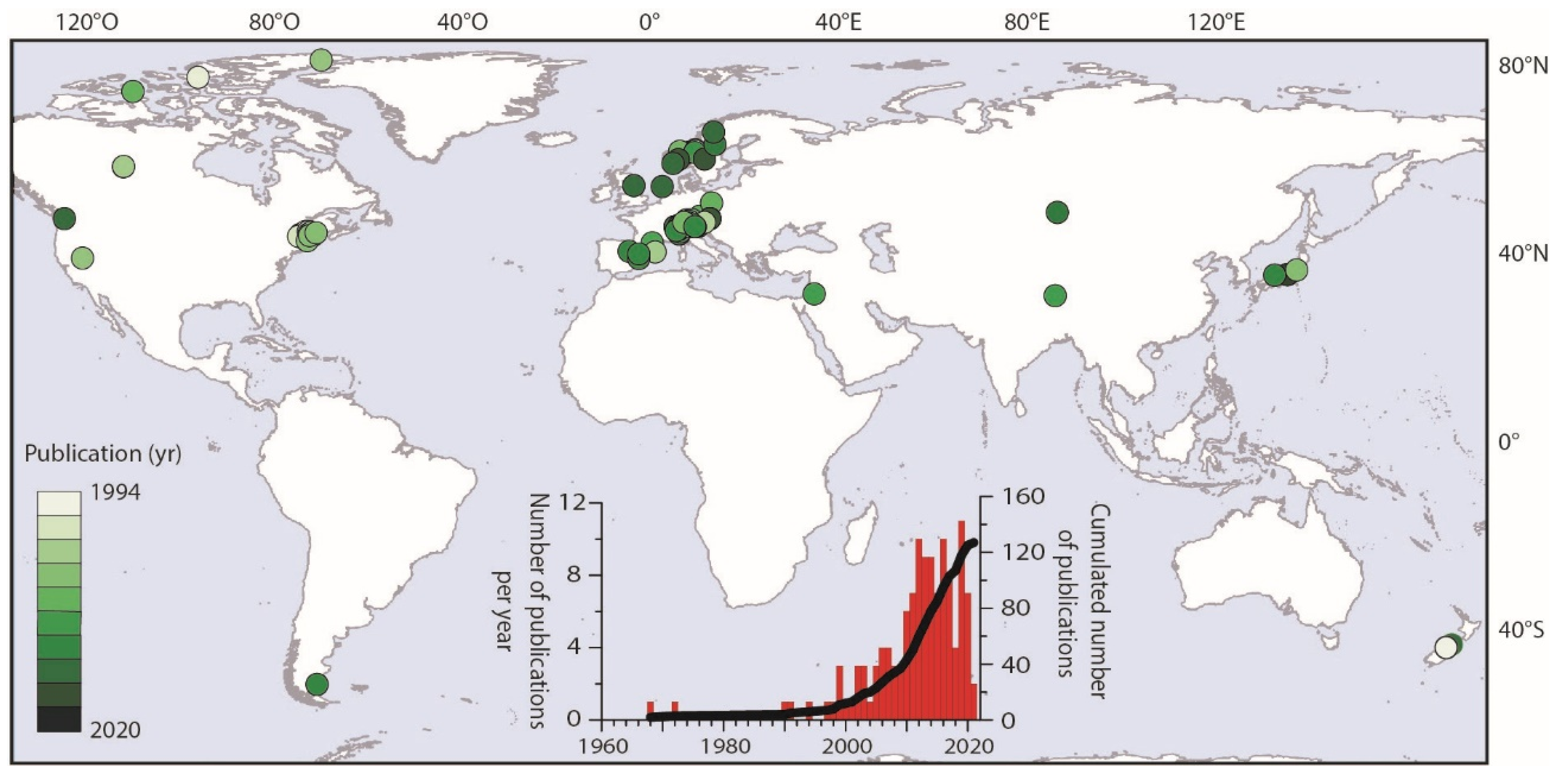
The imprint of flood events in lake sediments and the related sedimentary processes have been first described at the end of the 19th century in Lake Geneva [9] and further documented only a century later in both lakes Geneva [10,11] and Thun [12]. At the turn of the 21st century, scientific efforts were mobilized to reconstruct the first flood series aiming to explore the climate-flood linkages over millennia in New Zealand [13,14], Norway [15], and America [16,17,18] (Figure 1). This inspired the first phase of development in paleoflood hydrology using lake sediments, with studies mostly concentrated in Europe as reviewed by Gilli et al. [19] and Schillereff et al. [20]. During the following decade, paleoflood hydrology received fast-growing attention as illustrated by the three-fold publication increase (Figure 1), which resulted in the acquisition of extensive datasets, in the significant development of methodologies, and of hydrometeorological and statistical analyses aiming to better link changes in flood occurrence and magnitude with climate changes [21]. The present paper provides up-to-date and state-of-the-art knowledge on flood sedimentary processes and systems (Section 2 and Section 3), as well as on reconstructing (Section 4, Section 5, Section 6 and Section 7) and interpreting (Section 8) paleoflood records. Furthermore, we discuss possible perspectives in the field of paleoflood hydrology by highlighting the remaining challenges (Section 9).

2. Generation of a Flood Deposit

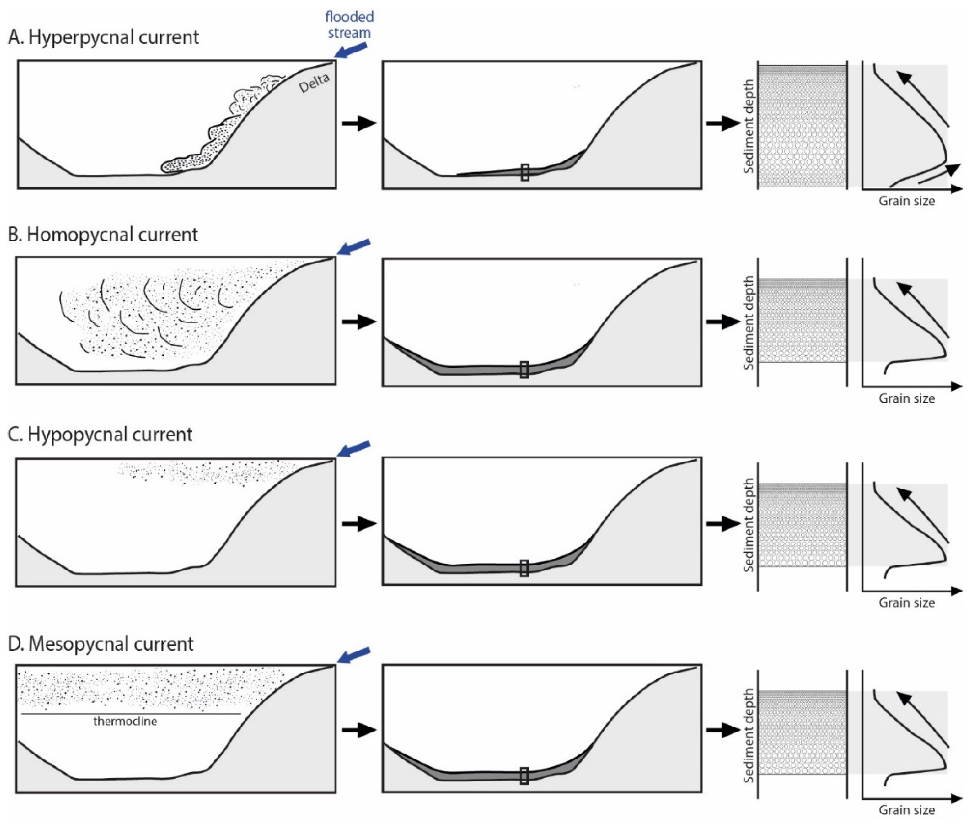
A flooding event usually implies overland flows and larger river discharge than usual, which have the potential to erode soil and riverbed particles. During these energetic events, the eroded particles are transferred from the source area (lake’s watershed) to the natural sink (lake floor) mostly via the river or other run-off processes. When the river enters the lake, the sediment particles are spread within the lake waters being mostly deposited on the lake floor (Figure 2). The pathways of this sediment-laden current strongly depend on the contrast between river and lake water densities, which are themselves mainly controlled by water temperature and suspended load. When the density of the sediment-water mixture from the riverine inlet exceeds that of the lake water, the mixture plunges and flows along the delta slopes as a land-derived hyperpycnal current [12,22,23,24] (Figure 2A). When the river and the lake waters are of similar densities, a rapid mixing of particles occurs throughout the lake water column, resulting in a homopycnal current (Figure 2B). On the other hand, when the river water density is lower than the standing lake water, the sediment plume is spread over the lake surface resulting in a hypopycnal flow [25] (see Figure 2 in Mulder and Chapron [22]). The lake water density also depends on its stratification conditions. Indeed, lakes can be thermally-stratified with warm, less dense waters in the upper part of the water column and both colder and denser waters in the lower part. Under these conditions, the river may not be dense enough to break through the lake stratification and through the sediment plume that is spread over the thermocline, thus resulting in a mesopycnal current [22,25,26,27,28] (see Figure 2 in Mulder and Chapron [22]). Homo- and hyperpycnal currents seem to be the most classical flood-induced sediment-laden currents (Figure 2), while hypo- and mesopycnal currents are less frequently observed.

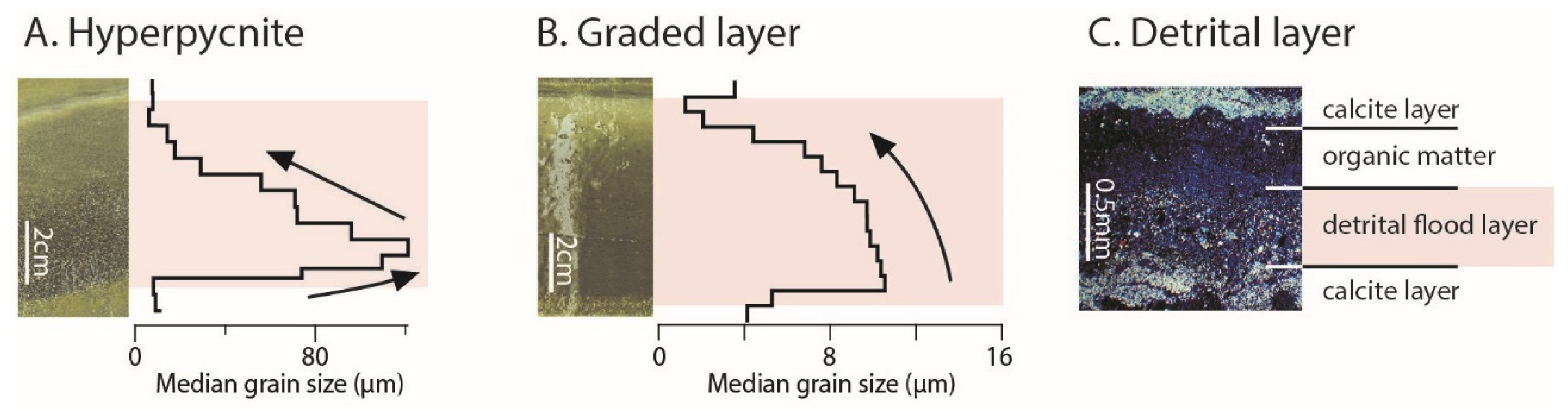
Flood-induced hyperpycnal currents are expected to be reflected in the lake deposits by a coarsening-upward basal sequence followed by a fining-upward upper sequence resulting from the waxing and waning phases of the river flow, respectively [22] (Figure 2A and Figure 3A). However, such a flood deposit is not really common in lacustrine environments [11,23,24,29,30,31,32,33,34,35,36,37]. Most of the time, only the upper, fining-upward sequence is observed and the deposits are thus commonly called graded deposits (Figure 2B and Figure 3B). The absence of the basal sequence may result from the high-energy currents during the flood peak, eroding the basal sequence as suggested by the erosional base of some graded deposits. Alternatively, Saitoh et al. [35] suggested that graded beds are the distal evolution of deposits resulting from flood-induced hyperpycnal currents. Lastly, thin flood-induced deposits can preclude the coarsening-upward sequence to be observed.

Following a meso-, hypo- or homopycnal current, a differential settling of suspended particles develops with respect to the different sizes of grains, which results in a fining-upward sequence resembling the upper sequence of a hyperpycnite, i.e., a graded bed (Figure 2B). These graded beds are all terminated by a fine light cap at the top that consists of clay particles that slowly settle when energy dissipates at the end of the flooding event. These graded beds differ from those resulting from hyperpycnal currents by the sharp but non-erosive base. Occasionally, these graded layers show a “patchy” lateral layer distribution that may be explained by internal lake currents during the particles settling, leading to a heterogeneous spatial layer distribution [38]. Homopycnal currents are frequent when the material available in the catchment is made of fine particles [24,39,40], such as for proglacial environments where clay-size glacial sediment is abundant [12,41,42,43]. Those layers induced by homopycnal currents are usually characterized by well-sorted particles and a deposit that is more largely spread out over the lake [24,25,44] (Figure 2B). A later type of flood deposit has often been described as thin, homogeneous silty, sandy, or silty-sandy detrital layers intercalated into a sediment matrix [15,17,18,38] (Figure 3C). This type of flood deposit has mainly been described for sites whose sedimentation is dominated by autochthonous inputs. That is, sites that are usually not or only slightly influenced by hydrology and/or erosive processes in the watershed. The depositional processes remain unclear. Whether meso-, hypo-, homo- or hyperpycnal currents, the specific generation of a flood deposit should thus make it possible to distinguish it from the background sedimentation in a lake sediment sequence.

3. Flood-Recording Systems

The record of flood deposits in a lake requires the availability of easily-erodible material in the catchment and a good transfer of this material through the catchment-lake system. This material can be the soils [45,46,47], fragile or weathered rocks [48] and deposits resulting for example from terrestrial landslide, alluvial or glacial activity [41,49,50]. The level of erodibility of this material may change the sensitivity of the catchment-lake system to record a flood event. The easier the material can be eroded, the more sensitive the catchment-lake system will be to record floods. This results in a highly different number of recorded floods, from a pluriannual [40,47,51,52,53] to a centennial [4,51] mean recurrence. Once eroded, the transfer of the flood material then depends on the river connectivity, e.g., an intermediate lake may act as a natural sediment trap [31,37]. Thereby, the presence of easily-erodible material along the stream and a well-developed delta are relevant indicators of good flood-recording systems, but they are not sufficient. Indeed, a rounded-shape delta suggests a highly changing river pathway that probably results in different underwater current pathways and thereby, in different flood deposit extends through time through time. This is clearly observed in the Rhone delta in Lake Geneva where a major (centennial) flood in the Swiss Rhone Valley completely modified the shape of the delta and its subaquatic channels, shifting northwards the pathways of the subsequent flood-related underwater currents for two centuries, until a more recent centennial flood shifted again the delta system [53]. These modifications in the delta sedimentary dynamics related to extreme floods eventually resulted in varying flood deposit geometries over time and, thereby, in a complex flood stratigraphy [11,53]. Therefore, recovering flood deposits then requires taking into account the size and morphology of the lake basin. For instance, in large lakes, only high-magnitude floods are powerful enough to disperse the sediments as far as the deep basins, which are the usual coring locations [54]. A proximal-distal transect of cores can then enable the whole variety of flood deposit positions to be covered [20,24,54,55]. Complex lake basin morphology may also result in a complex flood stratigraphy, especially if the sediment-laden currents change over time between hypo-, meso-, homo- and hyperpycnal (Section 2). Hypo-, meso- and homopycnal currents will tend to disperse the flood sediments over larger spatial extents whatever the lake basin morphology, while hyperpycnal currents follow the lake floor geometries such as channels and can be blocked by sills between sub-basins [30]. Lastly, the identification of flood deposits in a sediment sequence can be complicated by a low contrast between the flood deposits and the sedimentary background. Depending on the environmental setting of the catchment-lake systems, this sediment background can be either absent [47], detrital-rich [41,43] or authigenic-rich [54,56,57]. The absence of sediment background is the most critical since the entire sediment sequence is made of flood deposits, making the detection of flood deposit boundaries subtle. By contrast, an organic-rich sediment background is the most preferable since it will increase the contrast of nature with the flood deposits. Due to these different issues, not all lakes subject to flooding can reveal the presence of flood deposits. For instance, only 20 out of 35 cored lakes (56.5%) in the French Alps revealed flood deposits. Even sequences from neighboring lakes can record either plenty of floods or none [58]. With this in mind, the best-suited lakes for paleoflood reconstructions can exhibit well-developed deltas, but not round-shaped, and have a catchment with easily-erodible material and preferably located in a temperate setting to favor an organic-rich sediment background that would contrast with a flood signal. Furthermore, catchments with the presence of entities along the inflowing river that could act as an intermediate sediment trap (e.g., swamps, river plain or other small lakes) should be avoided.

4. Identifying Flood Layers

Flood deposits result from specific sedimentary currents, given specific features of grain size and spatial extent [59]. They also have a mineral composition that reflects the lithology of their watersheds, contrasting with the endogenic sedimentation usually more enriched in amorphous lacustrine organic matter and resulting in distinct colors and densities. The identification of flood deposits in a sediment sequence relies on these differences that can be determined using the following analyses. One should take care that, while below examples of the use of different proxies are given, they should not be directly used as a “cooking recipe”. A good knowledge of the system, i.e., of the geological substratum, in-lake processes and changes in environmental conditions, is required to identify the most appropriate proxies for flood identification. The combination of multiple proxies is also very useful and provides more robust interpretations.

4.1. Spatial Patterns (Stratigraphic Correlation from a Set of Cores)

Flood layers result from the deposition of sediments that have been transported within the lake by hypo-, homo- or hyperpycnal currents (Section 2). Each of these currents will result in different spatial extents of deposition. Deposits resulting from hyperpycnal currents generally cover areas from proximal locations up to the deep basin, while deposits resulting from hypo or homopycnal currents cover a larger area including for example the slopes opposite to the delta [22,24]. While the recognition of these processes is possible from monitoring [23,27,59], reconstructing them is only possible by sampling a set of cores from the different sedimentary environments (e.g., proximal area, deep basin, foot of lateral slopes) and performing the stratigraphical correlation of the flood layers from this set of cores [24,44]. A seismic survey, imaging the sedimentary infill, can be helpful to approach the spatial extent of flood layers and mass movements (Section 5), especially in large lakes where a very high number of cores may be needed to cover all sedimentary environments [45]. However, the acquisition of seismic data is sometimes difficult in certain sedimentary environments (e.g., gas blanking effect) and only reveals deposits thicker than several centimeters. The description of the spatial patterns of the deposits will highly help to distinguish flood layers among other event layers (Section 5) and find proxies of flood magnitude (Section 7).

4.2. Visual Description

Direct visual descriptions of sediment cores allow a rapid characterization of several key parameters of flood layers such as grain size, sorting, color, macroremains, layer thickness and morphologies and/or physical structures. Eye-naked sedimentological characterization often requires cleaning and smoothing of freshwater sediment with a metal spatula. Afterward grain-size, sorting and color can be qualitatively determined by direct comparison with standardized soil and sediment charts by finding best matches [60]. Colour should be determined immediately after the opening of the sediment core to avoid color alteration by drying and oxidation processes. Macroremains that are usually transported from the watershed during floods can also be visually identified, classified and used for radiocarbon dating, however, with caution as these macroremains may derive from mobilisation of very old material [48,58,61] (Section 6.1). Visual description of sediment cores is also an excellent approach to first identify macroscopic-scale physical and sedimentological structures in two dimensions (2D) that are diagnostic of the depositional processes and triggering factors such as erosional contacts, presence of slumps and folded material and/or liquefaction structures [37,62,63]. The 3D morphology of these structures can be subsequently investigated by high-resolution imaging techniques (i.e., CT scan, Section 4.3). Core pictures are obtained immediately after splitting the sediment cores in two halves and can be used to perform/refine sedimentological descriptions of the flood layers. On the other hand, the use of smear slides and thin sections retrieved from sediment cores allows for microscopic-scale observations of flood layers such as particle size or micro-facies variability [25,41,55,64] (Figure 4) that are difficult to recognize by visual descriptions. Smear slide observation is useful to qualitatively identify the mineral content, while thin sections can be used to determine the flood layers texture such as micro-erosional features, subtle grain-size variability and/or faint internal sub-layering [38,65,66,67]. Both, naked-eye “visu” and/or optical microscopy techniques are complementary and their use will depend on the thickness and structural complexity of the investigated flood layers.

4.3. Grain Size

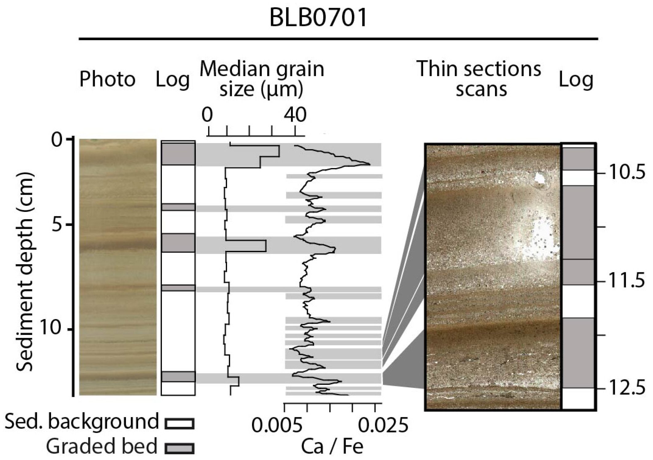
The particle size distribution (PSD) of the detrital matter that reflects the transport processes of allochthonous material towards and within the lake is a key feature of flood layers. The removal of the organic matter contained in the sediment samples is then a preliminary step of PSD analyses, usually performed with a bath of diluted hydrogen peroxide [39,68]. PSD is commonly measured using the laser diffraction method given the range of particle sizes [69]. The occurrence of flood layers is often expressed as an increase in mean grain size [33,70], caused by a higher sediment transport energy (Section 2 and Figure 4 and Figure 5). PSD can also reveal the coarsening-upward grading followed by the fining-upward grading typical of hyperpycnites or the unique fining-upward grading typical of graded layers. The sorting and PSD percentiles are other parameters helping to decipher the triggers of the graded layers [44,71], e.g., between floods or mass movements (Section 5). The recent development of core scanning techniques has permitted the acquisition of non-destructive, high-resolution proxies of grain size (Section 4.4).

4.4. Density

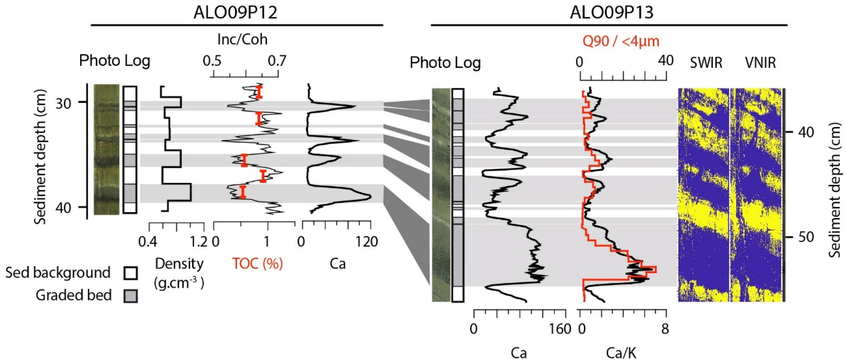
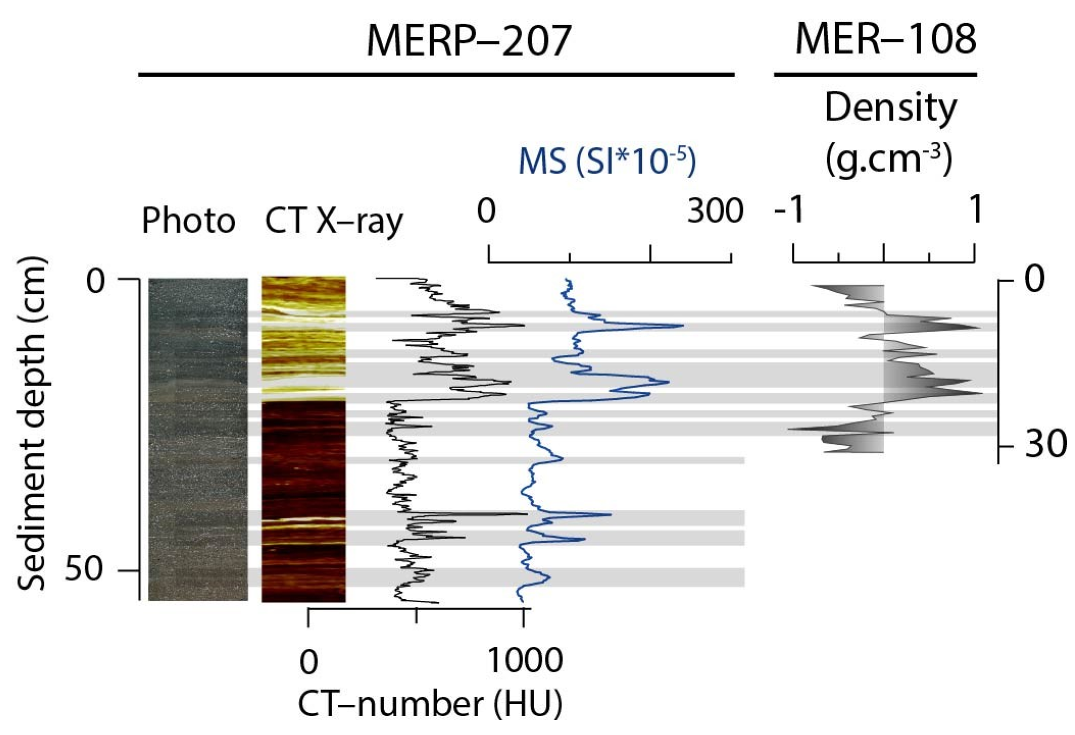
The high energy associated with river flooding often leads to the deposition of high-density material in lake sediments [13,41,72]. The density contrast in sediment core is enhanced for sediment background rich in organic matter [13,73]. Bulk density can be measured by sampling and weighting a known wet or dry volume of sediments (Figure 5). This method, however, requires a destructive sampling of the sediment cores and a minimum sediment sample size, which strongly limits both the sampling resolution (i.e., the detection of mm-scale flood layers) and the number of measured samples (i.e., the continuous measurement of long sediment sequences). These limitations have been overcome through the development of core scanning techniques that allowed for non-destructive, high-resolution measurements. Initially, multi-sensor core loggers (MSCL) were mounted with Gamma Ray Attenuation Porosity Evaluator (GRAPE) systems to provide a density estimate integrated over an irradiated cylindrical volume of sediment with a resolution between 2 and 5 mm [74]. Later, X-ray 3D computed tomography (CT) further improved the detection of flood layers on a sub-millimeter scale in a precise, fast and cost-efficient way, either by using medical [56] or industrial [73,75,76] CT scanners (Figure 6). Lastly, the use of the Coh/Inc ratio acquired by ITRAX core scanners can also be used as a non-destructive, high-resolution and continuous proxy for density [77] (Section 4.4).

4.5. Mineral and Isotopic Geochemistry

Sediments deposited during a flood event gather chemical and physical characteristics that can differ from the continuous sedimentation because of the different sediment sources and modes of deposition. Since the mineral and organic geochemical composition may then help identify flood deposits, geochemical analytical techniques were widely applied. Among these techniques, the XRF core scanning technique has been the most used, offering great advantages, such as time-efficient, continuous, and high-resolution (up to 100–200 µm) records without damaging the core (non-destructive method) [78]. It gives insight into the sediment elemental composition that can be used, depending on the sedimentary contexts, as proxy of:

(i)

Sediment origin. Flood layers are often enriched in lithogenic elements such as Ti, K, Rb, Ca and sometimes Zr (Figure 5). These elements can thus be used to distinguish mm-scale flood layers from the sediment background [79,80,81].

(ii)

Grain-size. Different geochemical composition between the finest (e.g., enriched in K and/or Fe) and the coarsest sediment fractions (e.g., enriched in Zr or Ca) were observed, allowing the robust reconstruction of mm-scale changes in grain size [43,47]. Then, these elements or rather elementary ratios such as Ca/K or Ca/Fe, Zr/Fe and Zr/K can be used as grain size proxies to identify flood deposits [38,43,47,61,82] (Figure 4 and Figure 5). The association between an elementary ratio and the grain size variability, however, needs to be tested and confirmed for each study site as it is bound to the mineralogy of the lake catchment and may also reflect changes in sediment origin or weathering processes. In addition, K might be preferred to Fe to represent fine particles in settings sensitive to redox processes.

(iii)

Organic matter (OM) content. By using the incoherence/coherence (Inc/Coh) ratio and the Br element, it is possible to distinguish the detrital-rich flood layers in organic-rich sediment sequences. The Compton (Inc) and Rayleigh (Coh) scattering are linked to the mean atomic number of the sample. Carbon-rich sediments generate high Compton and low Rayleigh scattering [83], which explains the relationship observed between the Inc/Coh ratio and the carbon content in some sediments [31] (Figure 5). Br is known to be incorporated into the biomass and is thus often correlated with the OM content [84,85,86]. Moreover, different relationships between the Br and OM were observed according to the source of organic material [86], making the Br/OM ratio potentially relevant for flood detection by distinguishing terrestrial from aquatic organic matter.

The different sources of material characterizing flood deposits from the sediment background have also been highlighted using stable isotopes. In carbonated settings, stable oxygen and carbon isotopes of bulk carbonates allow disentangling allochthonous (detrital) from autochthonous (endogenic) calcite [87]. Lastly, the combination of both scanning electron microscopy (SEM) and µ-XRF or energy dispersive spectroscopy (EDX) can further help distinguish flood layers from the continuous sedimentation, with a high 2D spatial resolution (<1 mm) [25,33,88,89]. While this combination of methods requires making a thin section or an impregnated sediment block and is thus destructive, it nevertheless allows determining the mineral composition of the deposits of interest and even the nature and size of their particles.

4.6. Magnetic Properties

Environmental magnetism, including the characterization of magnetic properties, holds the potential to differentiate between sediments with different magnetic signatures, and thus also fingerprint material mobilized by flood events. Magnetic susceptibility is a measure of a material’s ability to acquire magnetization when exposed to a weak magnetic field. Natural sediment samples are, depending on the carriers in question, composed of a mix of diamagnetic, paramagnetic and ferri/ferromagnetic particles [90]. When the sediment background is carbonated or organic, magnetic susceptibility measurements can be used to recognize flood deposits as minerogenic deposits with relatively high magnetic susceptibility or a rapid change in the sediment composition led by the minerogenic inputs during the flood [32,33,56,91,92,93] (Figure 6). Such measurements are typically done using a point sensor (Bartington MS2E) on a sediment core surface for 2 mm resolution measurements. The magnetic susceptibility can also be used to fingerprint different source materials given that they possess different magnetic carriers and that these have been stable over time [76,94,95,96]. For instance, Ekblom Johansson et al. [97] measured the mass specific magnetic susceptibility (χbulk) of sediment both at room temperature (293 K) and cooled (77 K) to differentiate between freshly-eroded glacial sediments and re-deposited flood transported sediments in a pro-glacial lake, using a Multi-Function Kappa Bridge (MFK1-FA). Given the temperature dependence of paramagnetic material, the ratio between χbulk77K and χbulk293K is used to study the influence of paramagnetic material on the bulk susceptibility. A high ratio (max 3.8) suggests that paramagnetic minerals dominate the sample, whereas a lower ratio indicates an increasing amount of ferromagnetic particles [98] and is directly related to the presence of freshly-eroded bedrock. Using this, Ekblom Johansson et al. [97] identified flood-transported material with relatively high ferromagnetic content, whereas the freshly-eroded glacial material was more paramagnetic. A similar approach was used by Støren et al. [92] to differentiate spring snowmelt floods from rainstorm floods, given that the different flood types mobilize material from different source materials.

4.7. Organic Matter

The high-energy transport of terrestrial sediments to the lake during floods may result in the presence of terrestrial plant macrofossils in the flood sediments, which is a classically used and easy-attributable feature of flood layers [32,93,99,100]. In detrital-rich lake sediment sequences, terrestrial inputs may be the main source of organic matter, resulting in high organic matter content in flood layers [32]. By contrast, in organic-rich sediment sequences, flood-induced detrital inputs often result in low organic content in flood layers [15,18,31,33,56,101]. Measurement of the organic content is commonly performed through Loss of Ignition [102] or Rock-Eval pyrolysis [103]. As introduced above, the Inc/Coh ratio or Br from XRF core scanner measurements can also supplant classical OM measurements for the benefit of time-efficient and high-resolution measurements [31] (Figure 5). Magnetic susceptibility has been used in a similar way, highlighting an increase of the mineral component at the expense of the organic one [32,33,93,101] (Figure 6). This, however, requires assuming that the magnetic mineralogy and the fraction of the magnetic particles within the detrital matter are stable over time. Further analyses of the organic matter can be carried out by quantitative organic petrography [104]. For instance, Simonneau et al. [45] revealed the presence of soils and lignocellulosic debris in flood deposits, contrasting with typical algal particles in background sediments. Rock-Eval pyrolysis [48], organic carbon isotopes δ¹³Corgb [33] and C/N atomic ratio [105,106] analyses also enable characterizing the lacustrine versus terrestrial origin of the organic matter when comparing its signature in bulk sediments and rock/soil samples from the catchment. Care is, however, required when interpreting higher δ¹³Corg values since they may also reflect higher algal productivity with eutrophication [107]. This change in quantity and nature of organic matter between flood deposits and sediment background induce color changes that can also be discriminated by visible-range [36,44,101,108] and short-wave infrared reflectance spectroscopic analyses [61].

4.8. High-Resolution Imaging and Automatic Detection of Flood Layers

The development of fast and non-destructive high-resolution acquisition techniques helps to improve flood layer detection. As for CT- and XRF-scans, high-resolution imaging techniques (HSI) can be used to highlight physical and chemical differences between the continuous sedimentation and the event layers. HSI analyzes the color of the sample surface using imaging sensors (visible near-infrared, VNIR: 400–1000 nm, and short wave infrared, SWIR: 1000–2500 nm). HSI can be combined with machine learning to characterize mineralogical fingerprints, organic matter and grain-size distribution at a very high sampling resolution, i.e., 60 to 200 µm [109,110] (Figure 5). It is thus a perfect tool to detect detrital input or coarse and graded beds from the continuous sedimentation and it can be used to identify flood layers. On the other hand, CT scanning (Section 4.3) allows exploration of complex sedimentary structures through sub-millimeter scale 3-D reconstructions based on differences in the relative densities of the observed objects [50,76,111]. From the 3-D numerical model, the image analysis can be used to obtain quantitative information about the grain-size, the organic matter content, erosional boundaries, the presence of macrofossils or the volumetry of objects [76], allowing to distinguish event layers from the continuous sedimentation [50,112,113].

The detection of flood events in a sediment sequence can be time-consuming and, depending on the methodology applied, characterized at a low resolution possibly leading to under-estimated identification and/or misidentification. The operator may need to combine several analyses to detect flood deposits. A few studies have developed semi-automatic or automatic methods to objectively detect flood deposits in a sedimentary sequence. High-resolution analytical approaches such as X-ray fluorescence spectroscopy, X-ray computed tomography, RGB images or hyperspectral imaging have been used to increase resolution and accuracy of the detection. A first attempt was made by Støren et al. [56], who used the rate of change of the magnetic susceptibility or of a CT-scan parameter. This value was calculated by dividing the variation in parameter values by variation in time. Vannière et al. [36] used an equivalent approach by extracting and normalizing the color signal from RGB images. For both studies, the methodology is rather simple, considering a flood deposit to be detected whenever the studied signal surpasses a threshold value. Recently, Rapuc et al. [109] showed that HSI, coupled with XRF data and discriminant algorithms, can also be used for high-resolution automatic identification of flood deposits.

Here, while the above examples of the use of different proxies are given, they should not be directly used as a “cooking recipe”. A good knowledge of the system, i.e., of the geological substratum, in-lake processes and changes in environmental conditions, is required to identify the most appropriate proxies for flood identification. The combination of multiple proxies is also very useful and provides more robust interpretations.

5. Flood Layers among Event Layers

The hyperpycnite is the only deposit unequivocal of the flood trigger (Section 2). Detrital, homogeneous layers and graded beds can also result from mass-movement-induced currents [31,44,58,71,114,115,116]. Disentangling the trigger of these deposits is thereby crucial but often challenging to reconstruct robust paleoflood series. The only straightforward criteria to associate them to its trigger is the case the layer is directly overlying a mass-wasting deposit (e.g., a slump) [39,43,93,117]. In most cases, the association to the trigger relies on a site-specific combination of clues based on the spatial pattern, textural features and composition of the event layers. The best case is the direct observation of in-situ mechanisms during events through the monitoring of the lake system [27,28,80] or the study of features of historically, well-documented events that can be used to decipher the trigger of older deposits [37,44].

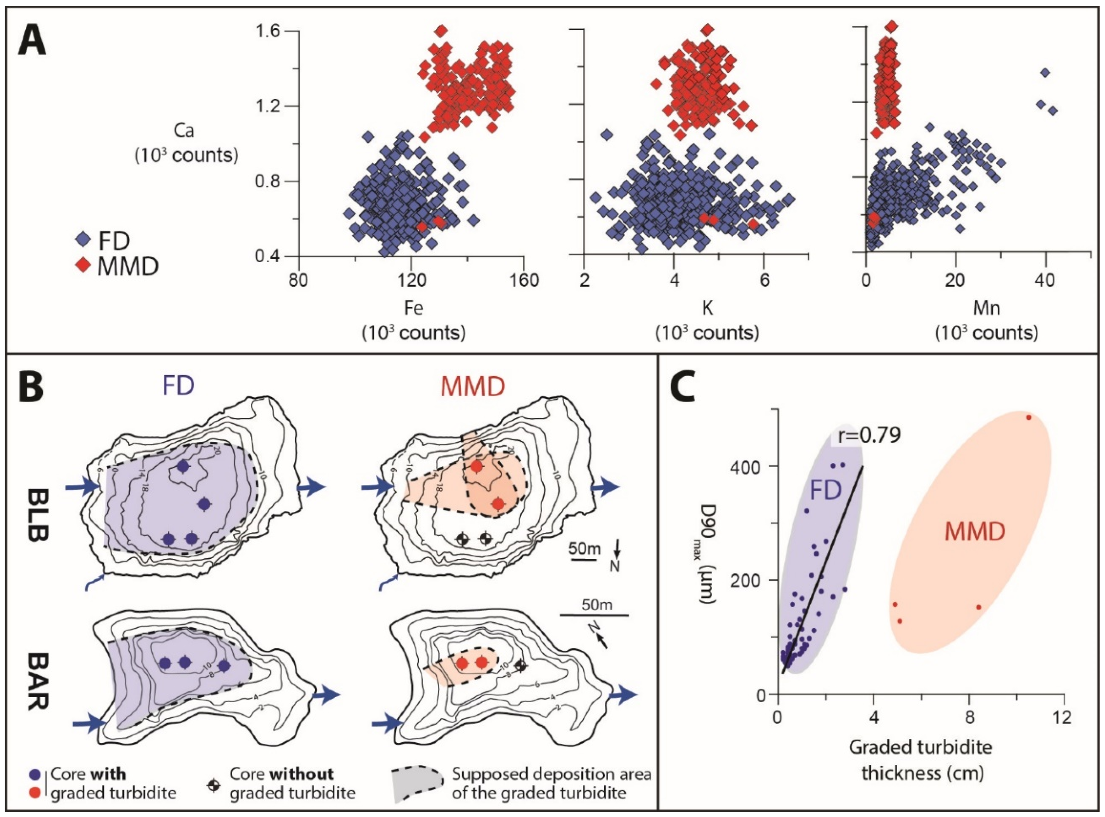
Studies often rely on the identification of distinct sediment sources since flood deposits are expected to be mainly composed of terrestrial sediments, whereas mass-movement deposits may be dominated by lacustrine sediments coming from the basin slopes (not influenced by the delta). All methods and tools used to detect flood layers in an organic-rich sediment sequence (Section 4) can thus be applied here to identify whether the event layer composition is closer either to the catchment material (i.e., flood deposits enriched in terrestrial material) or to the sedimentary background (i.e., mass-movement deposits enriched in lacustrine material). For instance, Simonneau et al. [45] showed with indicators derived from both Rock-Eval pyrolysis and quantitative organic petrography that mass-movement deposits mainly contain algal particles similar to those observed in background sediments, whereas flood deposits are made of soils and lignocellulosic debris. However, these methods and tools based on the contrast between terrestrial and lacustrine material are limited or even not applicable when (i) mass movements mobilize deltaic sediments, which are a mixture of both terrestrial and lacustrine sediments probably close to the flood deposit composition, or (ii) in detrital-rich environments, e.g., proglacial lakes, where the flood deposits and the sedimentary background are dominated by the terrestrial inputs. Complementary approaches based on source tracing can thus be implemented with analyses of the mineral geochemistry [11,39,100]. For instance, Wilhelm et al. [39] showed two clusters of deposits according to the geochemical features of the sediments; one made of material coming from the river catchment associated with flood deposits, and the other with features of lithologies located upstream from the lateral slopes associated to mass-movement deposits (Figure 7A). Beyond the classical elements analyzed to trace the sources (e.g., Ca, Ti, K, Fe), Mn has recently been shown to be a relevant, unequivocal indicator of the flood trigger. During a flood, oxygen-rich water coming from the watershed reaches the water-sediment interface. When lake-bottom waters are oxygen-depleted, the Mn present in dissolved form precipitates as Mn oxyhydroxides at the base of or within the flood deposits, where they are preserved. Thus, Mn can be interpreted as a proxy of flood-induced lake bottom oxygenation [39,61,109,118,119] (Figure 7A). Another complementary approach is to study sediment transport dynamics through the spatial pattern and grain size features of the flood deposits. The areal deposit extent reconstructed from a set of cores and seismic data can evidence the sediment source from either the deltaic or the littoral slopes, the latter being unequivocal of a mass movement trigger [41,45,115] (Figure 7B). In addition, deposits that are more evenly distributed over the entire lake basin are most likely to have been triggered by flood events, whereas mass-movement deposits tend to concentrate in the deeper parts [41,43,44,114,115]. Some grain-size parameters are also relevant indicators of the respective triggers. For instance, a higher sorting is expected in case of flood-induced currents [32,41,44,71,118,120]. A Passega-type diagram (median vs. a coarse percentile [39,121]) or sorting vs. mean grain size diagram [71]) that show how grain-size features evolve within the event layers helps to distinguish the ‘pure’ graded beds from the matrix-supported beds, especially when differences are too subtle to be detected through eye-naked observations [41,43,120]. Further scrutinizing of the ‘pure’ graded beds can be performed with plots of the basal coarsest fraction (D80 or higher) against the deposit thickness to disentangle the triggers [43,44,118,122] (Figure 7C). This analysis is based on the assumption that mass movements can transport large sediment quantities without an exceptionally high current energy, whereas sediment supplies and their grain size are both regulated by water currents during floods.

Whatever the context and the methods used, a latter clue is the synchronicity with known historical events. This requires both an age-depth model with minimal dating uncertainties and the access to an exhaustive collection of dates of modern and historical events able to trigger the flood deposits and mass movements (Section 6). The event-to-event comparison between dates of historical events and deposit ages can then support the inferred trigger [39,44,62,118].

Each catchment-lake system is characterized by its own geomorphological setting and related processes. The most suitable approach to take into account this diversity is to deploy the above-mentioned methods to get a set of potentially-relevant variables. As there is no unequivocal variable of triggers, the variables are not evidence but potential clues that should be considered altogether to see whether or not they converge towards a common trigger for each deposit. Once univocal proxies of their respective triggers are found, they can be used for an automatic identification of flood and mass-movement deposits. In this way, Vannière et al. [36] used color data reflecting distinct composition in an organic-rich sequence, while Rapuc et al. [109] used HSI and XRF-measured geochemical elements in a carbonate-rich sequence to distinguish flood from mass-movement deposits. Using a detrital-rich sequence from an Alaskan lake, Praet et al. [116] found that distinguishing event layers and their triggers could be more subtle. They used multivariate statistics with a large set of variables to show that basal grain-size and deposit thickness were the most effective proxies for this discrimination; thus confirming the previous finding from the Alps [43] (Figure 7C).

6. Reconstructing Paleoflood Occurrence

6.1. Dating the Flood Deposits

Reconstructing paleoflood occurrence from lake sediments, i.e.,, moving from identified flood layers to a paleoflood chronicle, requires the construction of a well-constrained chronology. Once the event layers are identified (Section 4), whether assigned to a flood event or a mass-movement turbidite (Section 5), they are considered instantaneous in the sediment age-depth modeling. Ultimately, their occurrence date can be extracted.

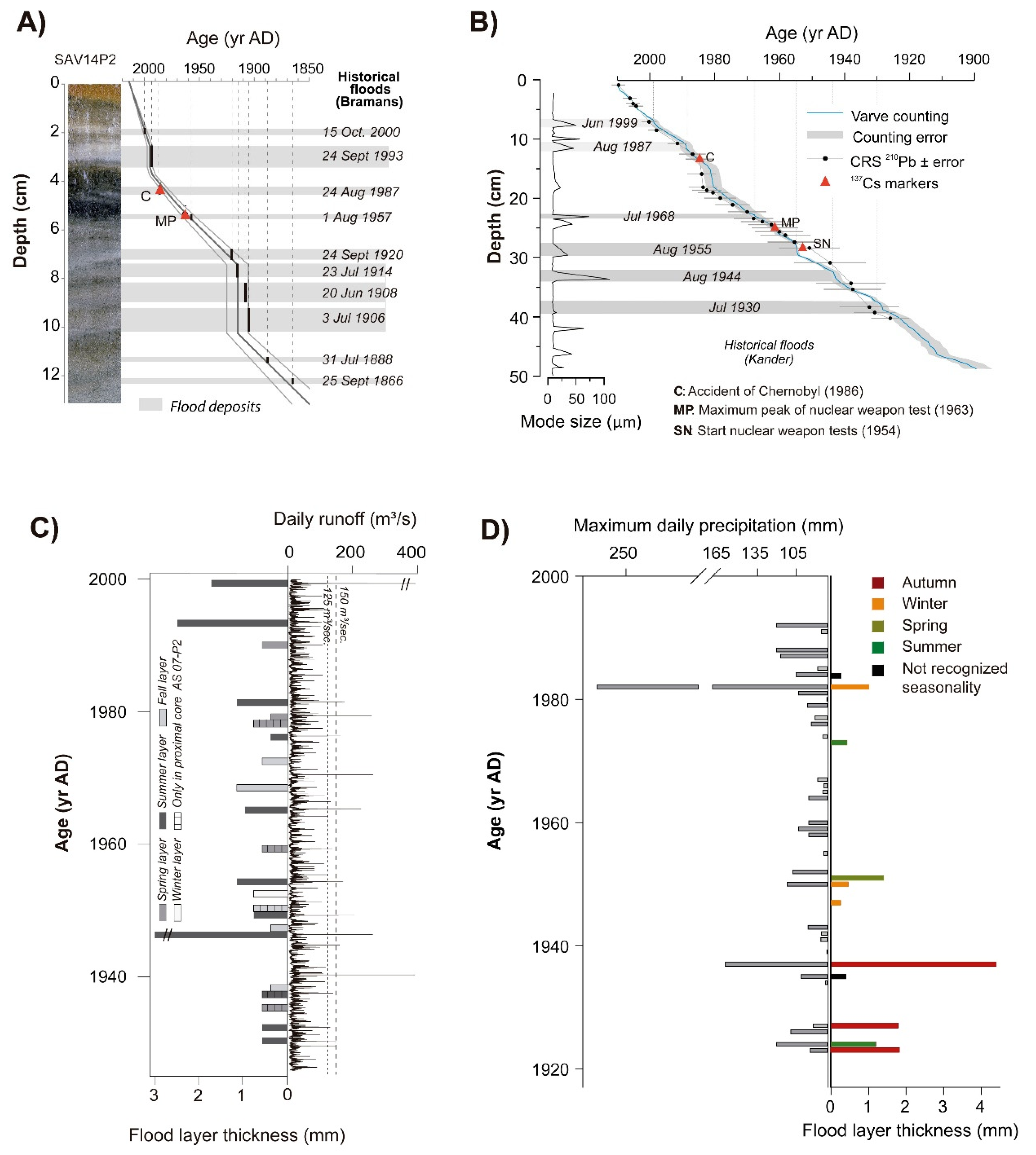
A wide range of dating methods, covering a large spectrum of time scales and uncertainties, can be used, either alone or, preferably, together in a concerted manner [19,21] (Figure 8). Over the last centuries, chronologies of lake-sediment records are usually based on short-lived radionuclides; mainly ¹³⁷Cs, and ²¹⁰Pb profiling. ¹³⁷Cs profiles allow to discriminate at most four discrete chronomarkers associated with nuclear weapon testing (initiation in AD 1954, and maximum Cs fallout in AD 1963), and to the Chernobyl and Fukushima accidents (AD 1986 and 2011). In contrast, ²¹⁰Pb dating technique requires an age-depth model, whose computation is subject to the selected assumptions with respect to ²¹⁰Pb_excess fluxes and sedimentation rates. More details about these models (such as CFCS, CIC, CRS, and CRS piecewise), their assumptions and applications have been recently reviewed by Bruel & Sabatier (2020) [123]. Chronologies of lake-sediment records covering longer time scales (i.e., millennia) are commonly based on radiocarbon (¹⁴C) dating of terrestrial plant macroremains. It is important to note that radiocarbon analyses should be preferably performed on macroremains coming from the sediment background. Indeed, macroremains in event layers may derive from mobilisation of very old material. Important progress of this method has considerably reduced the measurement uncertainties and the minimum recommended sample weights, where samples containing as little as a few micrograms of carbon can be dated using the gas-source input of the recently developed MIni CArbon DAting System (MICADAS). The usefulness of miniature samples (<150 μg C) was recently assessed for the dating of lake sediments [124]. Still marked by large uncertainties, ¹⁴C dating can be supplied by event stratigraphy to incorporate independent chronomarkers (e.g., human impact, earthquakes and volcanic eruptions). Furthermore, the matching between elementary geochemical stratigraphy and knowledge about catchment history of mineral ore production or regional/global lead pollution has been used to generate additional chronological control [22,125,126,127]. Secular variations in the paleogeomagnetic field have also been explored as a complementary tool to establish more robust age–depth relationships, allowing to reduce radiocarbon-induced dating uncertainties by up to 30% [128]. The principle behind palaeomagnetism-based chronologies consists in identifying synchronous variations of declination and inclination of the Characteristic Remanent Magnetization (ChRM) measured in the sediment records and the reference geomagnetic model. Combining different dating techniques help to reduce and constrain dating uncertainties. This is fundamental to be able to calibrate the flood chronicle to instrumental and historical series, and to accurately assess spatial changes in flood occurrence through the comparison with other regional paleoflood records. Such comparisons also require the construction of an accurate age-depth model, which considers event layers as instantaneous deposits (few hours or days) with respect to the background sedimentation (deposited at a much lower pace). In order to do so, different age-model computation techniques are offered, which include serac for the last century [123], and the widely-used CLAM, OxCal, Bacon and Bchron for longer periods, whose performance on lake sediments was recently reviewed by Trachsel and Telford (2017) [129].

Annually-laminated sediments, i.e., varved lake sediments, are considered here a particular case that offers two important advantages in paleoflood reconstruction using lake sediments: (i) the downcore counting of varves offers a direct and incremental dating technique with the highest possible chronological resolution [130], and (ii) the season of a flood can be identified in details through the relative position of the detrital layer within a varve year [52,64,89,131,132] (Figure 3C and Figure 8B). Due to the sub-mm scale of the deposits, varves and detrital layers are commonly discriminated using high-resolution microfacies sampling methodology, for which thin sections are analyzed with a petrographic analysis [68,132,133,134]. These microfacies observations can be reinforced by digital image analysis [135], high-resolution CT scan [75] or micro X-ray fluorescence analysis, which stand as powerful layer characterization and counting tools [27,64,131,136]. Once the varves and instantaneous deposits are well distinguished, a varve chronology is established through replicate varve counts and thickness measurements [130]. The uncertainty envelope can further be reduced by counts operated on multiple cores spatially distributed in the lake [64]. The chronology then needs to be validated, i.e., by confirming the annual character of the laminations all along the sequence. This is done through age consistency with other independent dating techniques, such as with ²¹⁰Pb and ¹³⁷Cs for upper sections, and with ¹⁴C dating and well-dated anchor points (historical floods, earthquakes, volcanic eruptions) for deeper sections of the sediment cores [68,131,133].

6.2. Calibrating the Record of Flood Occurrence

Improvements in flood layer detection and dating allowed producing detailed paleoflood chronicles [21], and made possible the calibration through event-to-event comparison with in-situ instrumental [26,27,28,38,54,64,122,126,127,131,135,137,138,139,140,141] (Figure 8C,D) and historical data [39,41,54,68,72,76,93,118,127] (Figure 8A,B). This calibration step first aims to validate the correspondence between flood layer deposits and observed flood events, and to quantify the degree of completeness of the flood record. Ideally, flood layer occurrence should be compared with discharge data from gauged stations close to the lake´s inlet, or at least from the same watershed. When this is not possible, rainfall data from nearby meteorological stations can be used as an indirect proxy for flood generation. Due to their low dating uncertainties, varved sediments make the event-to-event calibration possible at a seasonal resolution. This also makes it possible to assess the seasonal sensitivity of the lake to record floods [141] since flood-prone preconditioning factors may vary throughout the year [40]. For non-varved records, the event-to-event comparison may then be made difficult by the dating uncertainties. Although allocating specific flood layers to historical floods can be relatively well constrained over the last centuries as favored by the combination of dating techniques, the larger error range of millennial-long age-depth models might further challenge the comparison [126]. In this case, historical flood discharge peaks and identifiable flood deposits are often compared through periods of clustering in flood occurrence, such as through flood-rich vs. flood-poor periods [24,126,138]. Eventually, the resulting times series of paleoflood occurrence can be examined through correlation, clustering, frequency and cyclicity [132], and the comparison with local historical events and with other long-term flood or climatic records enables to investigate the general patterns of extreme hydrological events with respect to regional climate change.

7. Reconstructing Paleoflood Magnitude

7.1. Proxy of Flood Magnitude

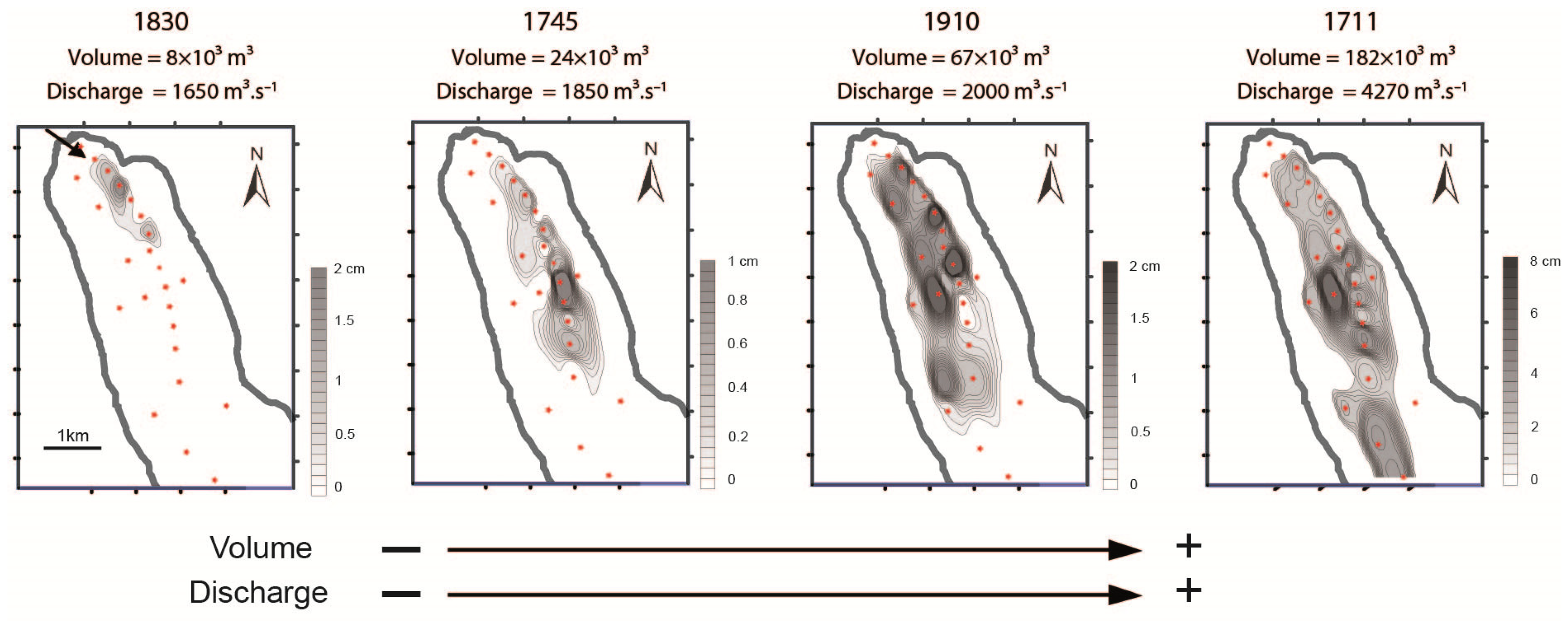
Reconstructing magnitude from lake sediments requires finding a relevant, site-dependent proxy due to the unavailability of direct evidence. A flood event is characterized by an exceptional increase in river water discharge, thus a greater energy for sediment erosion and transport. This can result in the transport of coarser particles [70,135] and larger sediment volumes [13,141,142] than under normal conditions. As such, one can expect that the higher the flood discharge, the coarser and the thicker the flood deposit [23,43]. The grain size [26,47], the deposit thickness [13,24,27,28,39,41,54] or both [43,118] can then be used as proxies of flood magnitude. Using grain size to quantify flood magnitude requires that the source of material in the catchment covers a wide range of grain sizes to reflect that of the flood discharge [24]. For instance, grain-size may be inappropriate to track changes in flood magnitude in the case of a clay-rich sediment source since all flood deposits are likely to be composed of similar fine particles [39]. This also requires measuring the coarsest fraction of each flood deposit since it is expected to reflect the flood peak. However, these measurements are time-consuming in flood-rich sediment sequence and limited to deposits thicker than a few millimeters due to the relatively low resolution of the analysis. To overcome these limitations, high-resolution geochemical data obtained through scanning techniques can be used as a proxy for grain size (Section 4), and/or for deposit thickness when the thickness is correlated to the grain size [24,43,72,118]. The deposit thickness can also be used to reconstruct flood-induced sediment volumes. For instance, Page et al. (1994) [13] observed a strong and significant correlation between total rainfall accumulated during storm events and deposit thickness in cores of lakes Tutira and Waikopiro, in New Zealand. However, the link between the deposit thickness in a given core and the total flood-sediment volume strongly depends on each site’s characteristics and, thereby, requires to be validated for each site. Indeed, the pathway of sediment-laden currents within the lake can vary between floods [23,50,54,59], thus resulting in various deposit geometries, even in case of similar flood discharges [24,27,54] (Figure 9). A multi-coring approach is the only way to account for these changing pathways and to reliably reconstruct the total sediment volume [54] (Figure 9). This issue of changing pathways is less problematic in lakes dominated by homopycnal currents, since a more homogeneous dispersion of the flood sediments within the lake basin is expected [24,41,43] (Figure 7B).

7.2. Calibrating the Record of Flood Magnitude

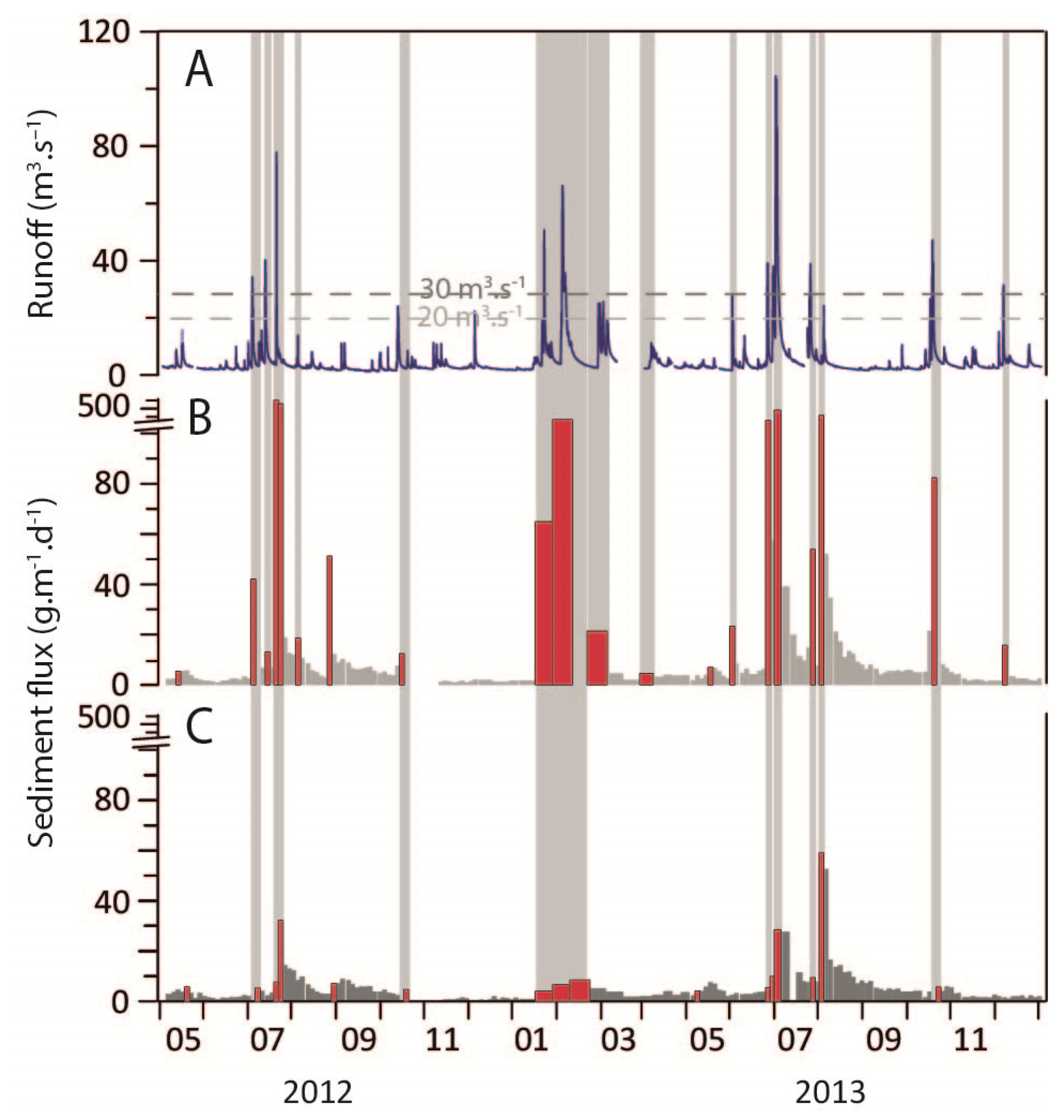
Any proxy of flood magnitude requires calibration. Similarly to flood occurrence, discharge data from gauged stations close to the lake´s inlet should be favored, or at least from the same watershed. When this is not possible, rainfall data from nearby meteorological stations are often used as an indirect proxy for flood generation. Such approaches have revealed site-specific thresholds in river and rainfall discharge, and they have provided insights into return periods of identified flood layers [6,26,38,54,64,80,141]. These calibrations and thresholds in peak discharge and/or maximum precipitation regimes are strictly dependent on the coring location, with river-proximal sites having a lower hydrological threshold than distal locations [27,28,54,64,80,127]. The hydrological thresholds within a given lake can be quantified through the deployment of a monitoring system combined with a multi-core sampling. Among the best examples is the monitoring of Lake Mondsee (Austria) by Kämpf et al., (2015, 2019) [28,87]. In this study, moorings were equipped with sediment traps and deployed in the lake at river proximal and distal locations, also integrating the upper and lower water column. This approach allowed characterizing the 3D spatial distribution of sediment fluxes in the lake water body through time to understand the flood layer formation in detail and to fix the hydrological threshold according to the coring locations (Figure 10). Thus, a careful selection of coring sites has been recommended, ideally integrating proximal and distal locations to obtain the most comprehensive record of flood events, i.e., documenting both small and large floods [27,28,54,64,72,141]. Jenny et al., (2014) [54] provide one of the best examples of flood magnitude reconstruction based on sediment volumes. They took advantage of a 150-year-long discharge series to transform flood-sediment volumes in maximal discharge (flood peak) back to 1650 (Figure 9). This calibration also allowed determining the discharge threshold for which a flood deposit can be observed in Lake Bourget (France) sediment sequence, i.e., to quantify the lake sensitivity to record floods. A similar discharge threshold has been quantified in Lake Gomma (Norway), and a 6000-year-long record of flood occurrence exceeding this minimal discharge value was produced [73]. In the case of lakes Bourget and Glomma, the threshold discharge is controlled by a natural sill. However, all lake systems containing flood deposits are characterized by a specific threshold. This is well illustrated by the facts that: (i) flood deposits are occasional in the sediment sequence, and (ii) the number of recorded flood deposits differs significantly between lake records (Section 3). The threshold mainly depends on the level of material erodibility in the catchment and the river capacity to the sediment transfer. In absence of monitoring and/or discharge data, historical data can help validate the proxy reliability as the coarsest and/or the thickest flood deposits are expected to correspond to the most severe documented flood events [41,72,118]. However, calibration studies of flood magnitude proxies from lake sediments remain rarely achieved because long discharge series, and historical data to a lesser extent, are rarely available directly from the studied lake catchments. That is the reason why, in most cases, flood-magnitude proxies provide information about the relative flood magnitude rather than absolute values, i.e., to document when floods were the most severe in a given catchment [24,39,73]. Another critical issue when dealing with sediment volumes as a proxy for flood-magnitude is related to changes in erosion processes over time. Long-term changes in geomorphology (e.g., landslides, glacier activity), vegetation cover and human activity in a lake catchment can change the availability of material to be eroded and, thereby, can alter the relationship between discharge and sediment volumes. Therefore, the stability of erosion processes (Section 8) and, thereby, of the flood-magnitude proxy over time should be addressed.

8. Understanding the Drivers of the Paleoflood Records

Once a paleoflood chronicle is reconstructed, the following steps consist in constraining our interpretation of the record by (i) defining what are the characteristics and the hydrometeorological drivers of the recorded floods, and (ii) estimating the persistence of these drivers over the entire record.

8.1. Hydrometeorological Drivers

Understanding the characteristics (e.g., seasonality, discharge threshold, return periods) of the recorded floods and their hydrometeorological drivers is a prerequisite for a meaningful interpretation of flood occurrence and magnitude, and for relevant comparison with other hydrological records. Indeed, floods result from a complex combination of atmospheric, catchment and river network processes [2,143]. The variability in these processes may result in very different amounts of recorded floods between catchments, even in neighboring catchments subject to similar hydrometeorological conditions but that are characterized by different geophysical settings [143]. Ideally, this knowledge can be gained by analyzing the hydrometeorology of recently observed floods that occurred on the studied river [118,144]. Only a comprehensive instrumental dataset allows explaining the respective role of the atmospheric, catchment and river network processes. Regional flood typology [143] and climatology [145] can also help define the recorded floods and their drivers at first order. For instance, the flood seasonality is an important hydroclimate flood characteristic linked to the seasonality of the drivers [146]. This is easily accessible through the comparison with instrumental and/or historical data (Section 6), and can further be facilitated by the presence of varved sediments (Section 4). Beyond the seasonality, the comparison with long instrumental series or historical data from the same river can be used to date the occurrence of recently recorded floods with a daily resolution. Such information may be combined with long reanalysis datasets such as NCEP-NCAR Reanalysis [147] and 20th Century Reanalysis [148] to determine the hydrometeorological processes triggering the recorded floods [5,120,149]. Reanalysis datasets are also used to explore the relationship between large-scale atmospheric patterns and flood occurrence by studying changes in flood frequency and the variability of atmospheric circulation [5,52,118,150,151]. This comprises atmospheric blocking through high-pressure fields [5,151], shifts in atmospheric circulation and pressure variations [150], and the importance of cyclonic weather types and advective flows in initiating hydrological extremes [52,152]. Thus, improving our knowledge about flood-relevant atmospheric circulation changes, and the respective contribution of convection and advection in the generation of a flood [118] is key to discuss the reliability of regional paleoflood compilations. Furthermore, stacking paleoflood records of various flood types can bring insights into regional flood patterns and potential large-scale drivers [4,18,51]. Such an approach can also help detect similarities (differences) in the hydrometeorological processes due to synchronous (asynchronous) changes in past flood frequency and magnitude [150,153]. However, before extrapolating the hydrometeorological features to the past and using modern floods as analogues of past ones, the stability of the sedimentary processes within the catchment lake system needs to be evaluated beyond the instrumental period. Assessing the relative impact of the different drivers on past erosion conditions can address this challenge [153].

8.2. Long-Term Effect of Catchment Modification

When the sedimentary processes change over time, this may result in a different link between the hydrometeorological drivers and the recorded floods. For instance, a temporary increase in easily-erodible sediment availability in the catchment area can result in more frequent and thicker flood deposits since floods smaller than usual can erode and transport sediments toward the lake [50]. Any change in the catchment geomorphology, the vegetation cover and/or the land use may modify the sediment availability in the catchment area and disturb the relationships to the hydrometeorological drivers.

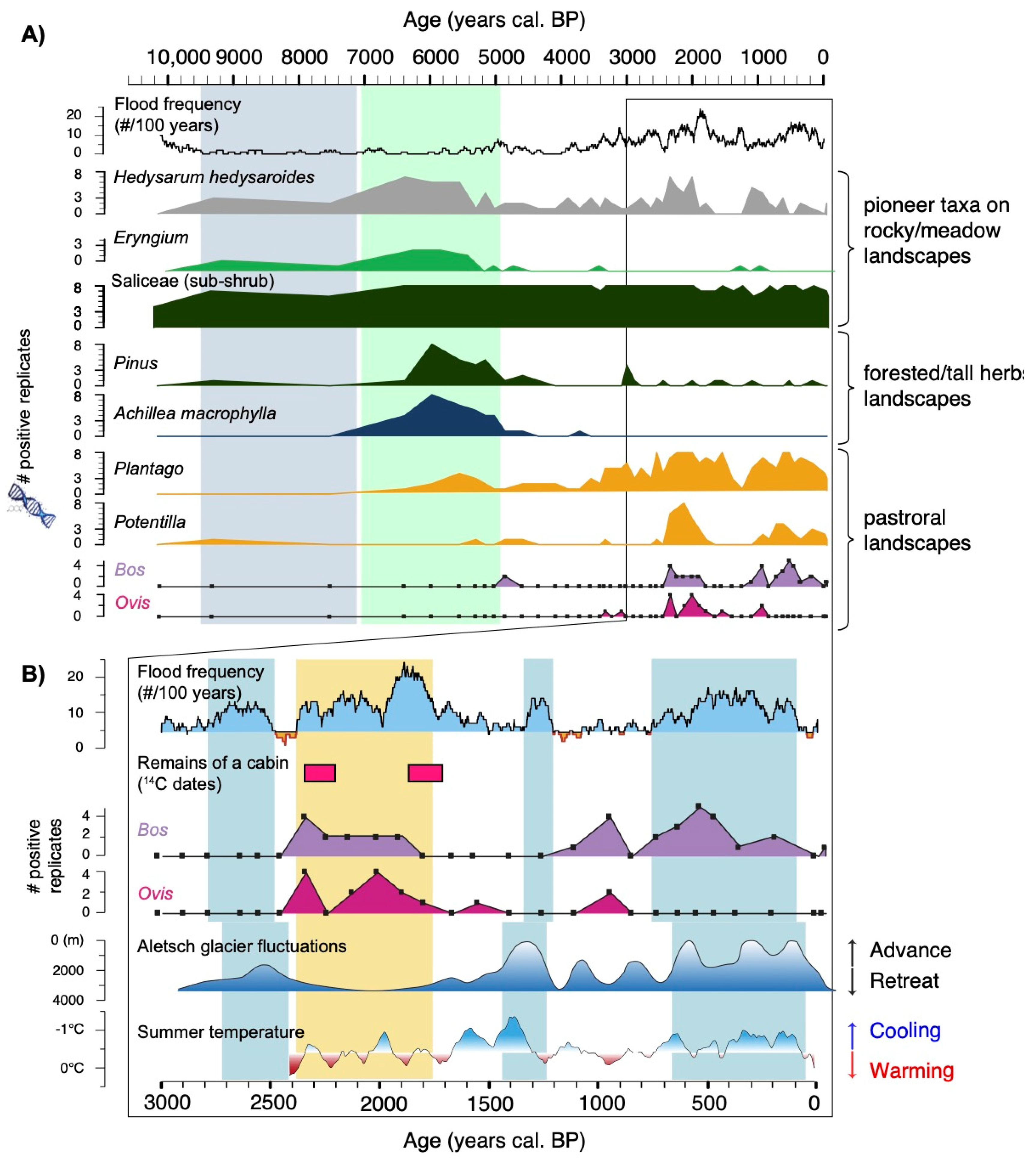
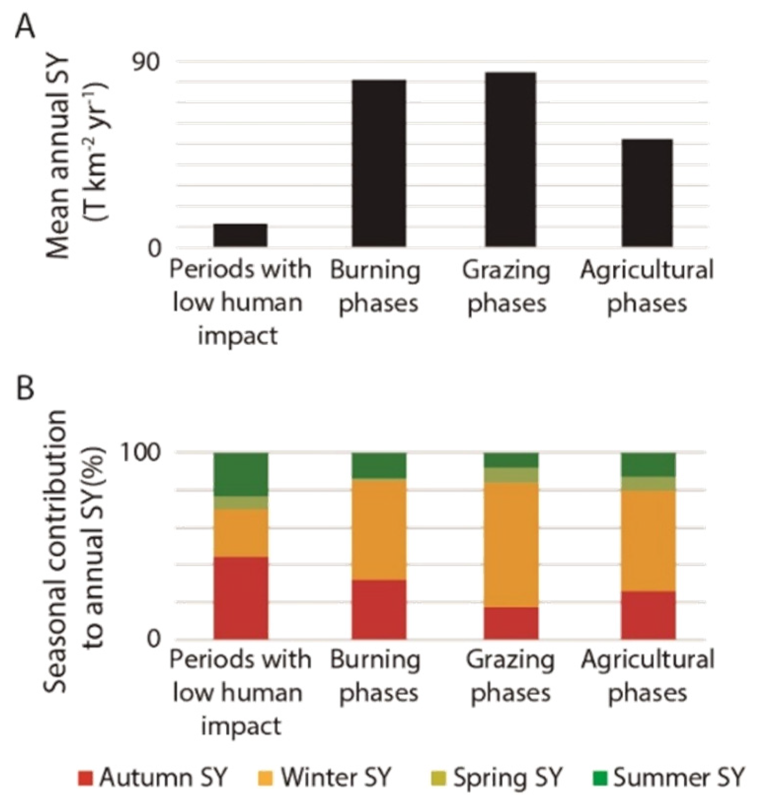
The geological and geomorphological map of the catchment area helps identify current and past sources of sediments, while historical and/or paleo-information can help document their possible changes in time. For instance, a threefold increase in flood-sediment flux has been observed in Lake Paringa (New Zealand) at the time of large seismically-induced landslides [49]. Similarly, glacial activity has been identified as a factor of changing sediment availability, constantly changing the relationships between climate and recorded floods [50]. However, the glacial activity seems to play a minor role as soon as there is a pre-existing, large stock of glacial material in the catchment [41,43,68]. The vegetation cover may change over time following natural environmental and climatic changes. For instance, following the glacial retreat at the beginning of the Holocene, the restoration of the vegetation cover (from rocky environments to forested areas) and the soil formation leading to slope stabilization occurred during about a millennium [48,153]. Such natural processes reduced the sediment availability in the catchment and, thereby, the sensitivity of the catchment-lake system to record floods [48] (Figure 11A). The vegetation cover can also be impacted by changes in land use through different mechanisms depending on human activities. Deforestation destabilizes the soil structure and exposes these disturbed soils directly to rainfall events. Pastoral activities reduce the vegetation cover and increase the soil compaction through trampling. This leads to more particles being exposed to rainfall events, accelerates the surface runoff and thus increases the capacity of particle mobilization (Figure 11B). Agricultural practices (e.g., ploughing, use of pesticides) also favor the sediment mobilization. These effects have been well highlighted in the Lake Montcortès sequence, where the flood-sediment yield has been multiplied by 5 to 9 depending on the different practices in the catchment area [140] (Figure 12A). In addition, they also modify the seasonal distribution of the sediment inputs (Figure 12B). More generally, such human-induced modifications of the catchment-lake system have been observed to trigger either no impact on the flood record [25,55,72,101,118] or increases in both frequency and thickness of flood deposits [36,46,47,154] (Figure 12). Lastly, the establishment of agricultural terraces, of hedges to delimit plots or the way of planting (parallel instead of perpendicular to the slope) are expected to reduce the energy of the surface runoff and thus the capacity to mobilize particles during a rainfall event [155]. Humans can also act on the river course, modifying the sediment transfers during floods by for example building embankments or dams. For instance, in Lake Iseo catchment high and low flood frequencies were recorded during the Medieval Climate Anomaly (MCA) and the Little Ice Age (LIA), respectively [61]. Since flood frequency is known to regionally decrease (increase) during the MCA (LIA), the pattern recorded in Lake Iseo does not seem to be driven by climate changes. Instead, human activities may explain it with the abandonment of a village built on the delta at the beginning of the MCA, allowing the river to freely avulse. Then, during the LIA, a new village was built with flood protection infrastructures that divert the river course in a direction different from the coring site. However, the effects of such infrastructures are site-dependent, i.e., dependent on the initial, natural hydrological functioning, the modification carried out and its location as well as on the position of the studied sediment core. For instance, the building of dams and embankments upstream of Lake Bourget does not seem to have impacted the record of floods in its sedimentary sequence. Indeed, these infrastructures do not trap fine particles during large floods that were the only ones to reach the lake under both natural and man-made conditions [6,54]. Another remarkable example of river corrections affecting the sediment dynamics and flood record is very well seen in Lake Geneva where several engineering works during the last two centuries have strongly affected the Rhone river’s natural course upstream of the lake [156]. These river corrections have resulted in (i) the migration and deactivation of subaquatic channels that previously funneled flood-related hyperpycnal currents to the distal basin [53,117] and (ii) the impact on the erosion/sedimentation interplay in the active channel modifying the conduit morphology [157,158], eventually affected the completeness of the flood record in the distal basin [11].

Overall, changes in sedimentary processes due to human activities and settlements can thus have a significant impact on the flood record. Such processes should then be systematically taken into account to correctly interpret changes in flood frequency and magnitude. The most common analyses applied to obtain information on land use, and more generally on land cover, are palynological analyses (e.g., pollen, spores of coprophilous fungi) [36,140,162]. Pollen provides insights into the evolution of the forest cover (e.g., deforestation) and the development of crops based on the identification of taxa from cultivated fields (e.g., cereals, rye, buckwheat, hemp) or orchards (e.g., vine, walnuts, chestnuts). Palynological records also include nitrophilous and ruderal taxa associated with pastoral activities like Plantago sp., Rumex sp., Urtica sp. or Chenopodiaceae. These indirect proxies are also often complemented by the analyses of Sporormiella sp. spores growing on dejections from herbivores to validate the reconstruction of pastoral history [162,163]. However, vegetation reconstructions can reflect landscape changes over larger areas than those of the studied catchments because pollen can be transported by the wind over a great distance. To overcome this limit, plant DNA analysis from lake sediments (lake sedDNA) represents an interesting proxy. Indeed, it has been shown that runoff and erosion are the main transfer processes of plant DNA, thereby mainly coming from the watershed [164]. Lake sedDNA analyses also provide the opportunity to directly reconstruct the presence of livestock [46,164] (Figure 11B). However, while DNA analyses are powerful for examining the impact of different animal species on the dynamics of erosion and flood deposits, analyses of Sporormiella sp. spores are more sensitive for detecting weaker pastoral pressure and therefore potentially more subtle impacts on flood sedimentary dynamics [164]. The analysis of other biomolecules well preserved in the sediments, such as fecal molecules (stanols, bile acid), miliacin or cannabinol [165], may also provide key information on past human activities. Integration of such multi-proxy approaches on the same core is particularly relevant to assess the synchronicity between the phases of human activities and those of floods, without being affected by dating uncertainties (Figure 11 and Figure 12). However, multi-disciplinary approaches, including archaeology and history are also very useful to detect potential human impacts. For instance, in the case of the study of Lake Iseo, the unexpected pattern of high and low flood frequencies could only be explained thanks to the existence of archaeological data demonstrating the abandonment and building of the village on the delta during the MCA and LIA, respectively [61]. In another study on a small mountain lake (Lake Anterne in the northern French Alps), a phase of high flood frequency could be associated, not with a phase of high hydrological activity, but instead to a phase of high pastoral pressure based on a body of evidence including archaeological remains of a pastoral cabin containing sheep bones [161] (Figure 11).

9. Open Challenges for Improving Paleoflood Reconstructions and Their Uses

Providing long-term records of flood occurrence and magnitude, paleoflood data can inform flood design and flood risk assessment [2,3]. This is expected to (i) improve the estimation of the upper tail of the flood peak distribution [166], (ii) reduce the uncertainty of flood design [6], and (iii) provide scenarios of extraordinary floods [54]. In addition, integrating paleofloods can serve as an alternative path for estimating worst-case floods, such as the Probable Maximum Flood (PMF), which is required for safety considerations of high-hazard infrastructure in many countries. On the other hand, reconstructing paleofloods also offers the potential to better understand the processes that are associated with extreme events, and rarely documented by the short systematic gauge records. There is evidence that extreme floods can be generated by different processes than small floods [167]. The differences can reside in the atmospheric, catchment or river network processes [168,169,170]. Such applications are numerous in the literature using paleodata mostly based on riverine sediments [3] and much less on lake sediments because flood magnitude is rarely obtained from lake sediments. The main reasons are likely: (i) the absence of direct evidence for flood magnitude that requires complementary research to develop site-specific proxies, (ii) the significant effort needed for the acquisition of complementary data (continuous, high-resolution grain-size measurements or sediment volumes), and (iii) the lack of gauge records in the catchment of the studied lake for the proxy calibration (Section 7). On the other hand, even when paleoflood series document flood magnitude, there is some hesitation from the hydrology community and engineering practice to consider paleoflood information. This is in contrast to the recommendations made by some countries (e.g., USA, Australia and Spain) to incorporate paleoflood information in flood hazard assessments [171]. To tap into the full potential that paleoflood records can deliver for understanding, quantifying and managing flood risk, some challenges need to be addressed:

Given the stakes enumerated above, developing methods and applications to systematically document flood magnitude appears as a priority for the community. Therefore, we encourage to: (i) systematize case studies in gauged catchments to develop methods and identify their strengths, limits and conditions for replications, and (ii) acquire data for developing flood-magnitude proxies as often as possible. Ideally, these studies should be combined with monitoring and modeling endeavors to understand and quantify the complete path from the flood-triggering rainfall event through the catchment and river system to the lake sediments. This requires collaborations between sedimentologists, hydrologists and modelers.

The benefit of paleoflood data for flood design and risk assessment depends on the type (e.g., discharge magnitude or time interval during which a given discharge has not been exceeded), but also on the uncertainty of the paleodata. To decide whether the integration of a given paleo-dataset improves flood frequency estimation requires understanding its uncertainty. Therefore, particular care should be taken to identify, quantify and communicate uncertainties associated with the reconstructions (e.g., detection threshold, calibration, chronology, etc.).

A major obstacle for including paleoflood data into flood design and risk assessment is the argument of non-stationarity. Paleofloods may have occurred under climatic and land surface conditions which were so different from today (and from those in the near future) so that their transfer is questionable. Besides the counterview that paleofloods are important pieces of information despite potential non-stationarity, one should aim to understand the major drivers of change and the associated sensitivity of flood characteristics. For instance, flood timing, i.e., the occurrence of floods within the year, typically depends on climatic drivers and is not sensitive to land use. In contrast, flood magnitude can be sensitive to changes in atmospheric, catchment and river network processes. Reconstructions of climate and land surface characteristics (e.g., vegetation, geomorphology, soils) are important inputs to such analyses, which should be systematically considered. Developing relevant methods to analyze the interactions between climate, land surface and flood variability, taking into account the respective characteristics (e.g., time and space scales) and uncertainties, is another challenge.

The hypothesis that extreme floods are dominated by different (atmospheric, catchment, river channel) processes than the bulk of the flood events is a strong argument for using information about past extreme events in flood design and risk assessment. However, the strength of this argument hinges on the capacity to understand these processes and explain them mechanistically. Hence, future research should aim at understanding the hydrometeorological processes underlying paleoflood events and investigating whether extreme floods are dominated by different processes than small floods. Since this research question requires covering a broad panel of scientific knowledge and tools, interdisciplinary approaches including for example statisticians, climate and hydrological modelers should be developed.

References

- UNISDR; CRED. The Human Cost of Natural Disasters: A Global Perspective; Centre for Research on the Epidemiology of Disaster: Brussels, Belgium, 2015. [Google Scholar]
- Merz, B.; Aerts, J.; Arnbjerg-Nielsen, K.; Baldi, M.; Becker, A.; Bichet, A.; Blöschl, G.; Bouwer, L.M.; Brauer, A.; Cioffi, F.; et al. Floods and climate: Emerging perspectives for flood risk assessment and management. Nat. Hazards Earth Syst. Sci. 2014, 14, 1921–1942. [Google Scholar] [CrossRef] [Green Version]
- Wilhelm, B.; Cánovas, J.A.B.; Macdonald, N.; Toonen, W.H.; Baker, V.; Barriendos, M.; Benito, G.; Brauer, A.; Corella, J.P.; Denniston, R.; et al. Interpreting historical, botanical, and geological evidence to aid preparations for future floods. Wiley Interdiscip. Rev. Water 2019, 6, e1318. [Google Scholar] [CrossRef] [Green Version]
- Glur, L.; Wirth, S.B.; Büntgen, U.; Gilli, A.; Haug, G.H.; Schär, C.; Beer, J.; Anselmetti, F.S. Frequent floods in the European Alps coincide with cooler periods of the past 2500 years. Sci. Rep. 2013, 3, 2770. [Google Scholar] [CrossRef] [PubMed] [Green Version]
- Rimbu, N.; Czymzik, M.; Ionita, M.; Lohmann, G.; Brauer, A. Atmospheric circulation patterns associated with the variability of River Ammer floods: Evidence from observed and proxy data. Clim. Past 2016, 12, 377–385. [Google Scholar] [CrossRef] [Green Version]
- Evin, G.; Wilhelm, B.; Jenny, J.-P. Flood hazard assessment of the Rhône River revisited with reconstructed discharges from lake sediments. Glob. Planet. Chang. 2019, 172, 114–123. [Google Scholar] [CrossRef]
- Munoz, S.E.; Giosan, L.; Therrell, M.D.; Remo, J.W.F.; Shen, Z.; Sullivan, R.; Wiman, C.; O’Donnell, M.; Donnelly, J.P. Climatic control of Mississippi River flood hazard amplified by river engineering. Nature 2018, 556, 95–98. [Google Scholar] [CrossRef] [PubMed]
- Brunck, H.; Sirocko, F.; Albert, J. The ELSA-Flood-Stack: A reconstruction from the laminated sediments of Eifel maar structures during the last 60,000 years. Glob. Planet. Chang. 2016, 142, 136–146. [Google Scholar] [CrossRef]
- Forel, F.A. Les ravins sous-lacustres des fleuves glaciaires. C. R. Acad. Sci. Paris 1885, 1–3. [Google Scholar]
- Houbolt, J.J.H.C.; Jonker, J.B.M. Recent sediments in the eastern part of the Lake of Geneva (Lac Leman). Geol. Mijnbouw 1968, 47, 131–148. [Google Scholar]
- Kremer, K.; Corella, J.P.; Adatte, T.; Garnier, E.; Zenhäusern, G.; Girardclos, S. Origin of turbidites in deep Lake Geneva (France–Switzerland) in the last 1500 years. J. Sediment. Res. 2015, 85, 1455–1465. [Google Scholar] [CrossRef]
- Sturm, M.; Matter, A. Turbidites and varves in Lake Brienz (Switzerland): Deposition of clastic detritus by density currents. Spec. Publ. Int. Assoc. Sedimentol. 1978, 2, 147–168. [Google Scholar]
- Page, M.J.; Trustrum, N.A.; DeRose, R.C. A high resolution record of storm-induced erosion from lake sediments, New Zealand. J. Paleolimnol. 1994, 11, 333–348. [Google Scholar] [CrossRef]
- Eden, D.N.; Page, M.J. Palaeoclimatic implications of a storm erosion record from late Holocene lake sediments, North Island, New Zealand. Palaeogeogr. Palaeoclim. Palaeoecol. 1998, 139, 37–58. [Google Scholar] [CrossRef]
- Nesje, A.; Dahl, S.O.; Matthews, J.A.; Berrisford, M.S. A 4500-yr record of river floods obtained from a sediment core in Lake Atnsjoen, Eastern Norway. J. Paleolimnol. 2001, 25, 329–342. [Google Scholar] [CrossRef]
- Rodbell, D.T.; Seltzer, G.O.; Anderson, D.M.; Abbott, M.B.; Enfield, D.B.; Newman, J.H. An~15,000-year record of El Niño-driven alluviation in southwestern Ecuador. Science 1999, 283, 516–520. [Google Scholar] [CrossRef] [Green Version]
- Brown, S.L.; Bierman, P.R.; Lini, A.; Southon, J. 10,000 yr record of extreme hydrologic events. Geology 2000, 28, 335–338. [Google Scholar] [CrossRef]
- Noren, A.; Bierman, P.; Steig, E.J.; Lini, A.; Southon, J. Millennial-scale storminess variability in the northeastern United States during the Holocene epoch. Nature 2002, 419, 821–824. [Google Scholar] [CrossRef]
- Gilli, A.; Anselmetti, F.S.; Glur, L.; Wirth, S.B. Lake sediments as archives of recurrence rates and intensities of past flood events. In Dating Torrential Processes on Fans and Cones; Schneuwly-Bollschweiler, M., Stoffel, M., Rudolf-Miklau, F., Eds.; Springer: Dordrecht, The Netherlands, 2013; pp. 225–242. [Google Scholar]
- Schillereff, D.; Chiverrell, R.; Macdonald, N.; Hooke, J.M. Flood stratigraphies in lake sediments: A review. Earth-Sci. Rev. 2014, 135, 17–37. [Google Scholar] [CrossRef] [Green Version]
- Wilhelm, B.; Canovas, J.A.B.; Aznar, J.P.C.; Kämpf, L.; Swierczynski, T.; Stoffel, M.; Støren, E.; Toonen, W. Recent advances in paleoflood hydrology: From new archives to data compilation and analysis. Water Secur. 2018, 3, 1–8. [Google Scholar] [CrossRef]
- Mulder, T.; Chapron, E. Flood deposits in continental and marine environments: Character and significance. In Sediment Transfer from Shelf to Deep Water—Revisiting the Delivery System: Aapg Studies in Geology; The American Association of Petroleum Geologists and SEPM: Tulsa, OK, USA, 2011; pp. 1–30. [Google Scholar]
- Crookshanks, S.; Gilbert, R. Continuous, diurnally fluctuating turbidity currents in Kluane Lake, Yukon Territory. Can. J. Earth Sci. 2008, 45, 1123–1138. [Google Scholar] [CrossRef]
- Wilhelm, B.; Sabatier, P.; Arnaud, F. Is a regional flood signal reproducible from lake sediments? Sedimentology 2015, 62, 1103–1117. [Google Scholar] [CrossRef]
- Swierczynski, T.; Lauterbach, S.; Dulski, P.; Delgado, J.; Merz, B.; Brauer, A. Mid- to late Holocene flood frequency changes in the northeastern Alps as recorded in varved sediments of Lake Mondsee (Upper Austria). Quat. Sci. Rev. 2013, 80, 78–90. [Google Scholar] [CrossRef]
- Schillereff, D.N. A review of in situ measurement techniques for investigating suspended sediment dynamics in lakes. In Geomorphological Techniques; British Society for Geomorphology: London, UK, 2015. [Google Scholar]
- Kämpf, L.; Brauer, A.; Swierczynski, T.; Czymzik, M.; Mueller, P.; Dulski, P. Processes of flood-triggered detrital layer deposition in the varved Lake Mondsee sediment record revealed by a dual calibration approach. J. Quat. Sci. 2014, 29, 475–486. [Google Scholar] [CrossRef] [Green Version]
- Kämpf, L.; Mueller, P.; Höllerer, H.; Plessen, B.; Naumann, R.; Thoss, H.; Güntner, A.; Merz, B.; Brauer, A. Hydrological and sedimentological processes of flood layer formation in Lake Mondsee. Depos. Rec. 2015, 1, 18–37. [Google Scholar] [CrossRef]
- Schneider, J.-L.; Pollet, N.; Chapron, E.; Wessels, M.; Wassmer, P. Signature of Rhine Valley sturzstrom dam failures in Holocene sediments of Lake Constance, Germany. Sediment. Geol. 2004, 169, 75–91. [Google Scholar] [CrossRef]
- Chapron, E.; Juvigné, E.; Mulsow, S.; Ariztegui, D.; Magand, O.; Bertrand, S.; Pino, M.; Chapron, O. Recent clastic sedimentation processes in Lake Puyehue (Chilean Lake District, 40.5° S). Sediment. Geol. 2007, 201, 365–385. [Google Scholar] [CrossRef]
- Guyard, H.; Chapron, E.; St-Onge, G.; Anselmetti, F.; Arnaud, F.; Magand, O.; Francus, P.; Mélières, M.-A. High-altitude varve records of abrupt environmental changes and mining activity over the last 4000 years in the Western French Alps (Lake Bramant, Grandes Rousses Massif). Quat. Sci. Rev. 2007, 26, 2644–2660. [Google Scholar] [CrossRef]
- Støren, E.N.; Dahl, S.O.; Lie, Ø. Separation of late-Holocene episodic paraglacial events and glacier fluctuations in eastern Jotunheimen, central southern Norway. Holocene 2008, 18, 1179–1191. [Google Scholar] [CrossRef] [Green Version]
- Osleger, D.A.; Heyvaert, A.C.; Stoner, J.S.; Verosub, K.L. Lacustrine turbidites as indicators of Holocene storminess and climate: Lake Tahoe, California and Nevada. J. Paleolimnol. 2009, 42, 103–122. [Google Scholar] [CrossRef]
- Ito, T.; Iwamoto, H.; Kamiya, K.; Fukushima, T.; Kumon, F. Use of flood chronology for detailed environmental analysis: A case study of Lake Kizaki in the northern Japanese Alps, central Japan. Environ. Earth Sci. 2010, 60, 1607–1618. [Google Scholar] [CrossRef]
- Saitoh, Y.; Masuda, F. Spatial change of grading pattern of subaqueous flood deposits in Lake Shinji, Japan. J. Sediment. Res. 2013, 83, 221–233. [Google Scholar] [CrossRef]
- Vannière, B.; Magny, M.; Joannin, S.; Simonneau, A.; Wirth, S.B.; Hamann, Y.; Chapron, E.; Gilli, A.; Desmet, M.; Anselmetti, F.S. Orbital changes, variation in solar activity and increased anthropogenic activities: Controls on the Holocene flood frequency in the Lake Ledro Area, northern Italy. Clim. Past 2013, 9, 1193–1209. [Google Scholar] [CrossRef] [Green Version]
- Santos-González, J.; Gómez-Villar, A.; González-Gutiérrez, R.B.; Corella, J.P.; Benito, G.; Redondo-Vega, J.M.; Melón-Nava, A.; Valero-Garcés, B. Geomorphological impact, hydraulics and watershed-lake connectivity during extreme floods in mountain areas: The 1959 Vega De Tera dam failure, NW Spain. Geomorphology 2021, 375, 107531. [Google Scholar] [CrossRef]
- Corella, J.; Benito, G.; Rodriguez-Lloveras, X.; Brauer, A.; Garcés, B.V. Annually-resolved lake record of extreme hydro-meteorological events since AD 1347 in NE Iberian Peninsula. Quat. Sci. Rev. 2014, 93, 77–90. [Google Scholar] [CrossRef] [Green Version]
- Wilhelm, B.; Vogel, H.; Crouzet, C.; Etienne, D.; Anselmetti, F.S. Frequency and intensity of palaeofloods at the interface of Atlantic and Mediterranean climate domains. Clim. Past 2016, 12, 299–316. [Google Scholar] [CrossRef] [Green Version]
- Corella, J.P.; Benito, G.; Monteoliva, A.P.; Sigro, J.; Calle, M.; Valero-Garcés, B.L.; Stefanova, V.; Rico, E.; Favre, A.-C.; Wilhelm, B. A 1400-years flood frequency reconstruction for the Basque country (N Spain): Integrating geological, historical and instrumental datasets. Quat. Sci. Rev. 2021, 262, 106963. [Google Scholar] [CrossRef]
- Wilhelm, B.; Malet, E.; Allignol, F.; Legaz, A.; Giguet-Covex, C.; Magand, O.; Enters, D.; Arnaud, F.; Revillon, S. Does global warming favour the occurrence of extreme floods in European Alps? First evidences from a NW Alps proglacial lake sediment record. Clim. Chang. 2012, 113, 563–581. [Google Scholar] [CrossRef]
- Brodzikowski, K.; van Loon, A.J. Glacigenic Sediments; Elsevier: Amsterdam, The Netherlands, 1990. [Google Scholar]
- Wilhelm, B.; Arnaud, F.; Sabatier, P.; Magand, O.; Chapron, E.; Courp, T.; Tachikawa, K.; Fanget, B.; Malet, E.; Pignol, C. Palaeoflood activity and climate change over the last 1400 years recorded by lake sediments in the north-west European Alps. J. Quat. Sci. 2013, 28, 189–199. [Google Scholar] [CrossRef] [Green Version]
- Vandekerkhove, E.; Bertrand, S.; Mauquoy, D.; McWethy, D.; Reid, B.; Stammen, S.; Saunders, K.M.; Torrejón, F. Neoglacial increase in high-magnitude glacial lake outburst flood frequency, upper Baker River, Chilean Patagonia (47° S). Quat. Sci. Rev. 2020, 248, 106572. [Google Scholar] [CrossRef]
- Simonneau, A.; Doyen, E.; Chapron, E.; Millet, L.; Vannière, B.; Di Giovanni, C.; Bossard, N.; Tachikawa, K.; Bard, E.; Albéric, P.; et al. Holocene land-use evolution and associated soil erosion in the French Prealps inferred from Lake Paladru sediments and archaeological evidences. J. Archaeol. Sci. 2013, 40, 1636–1645. [Google Scholar] [CrossRef] [Green Version]
- Bajard, M.; Poulenard, J.; Sabatier, P.; Bertrand, Y.; Crouzet, C.; Ficetola, G.F.; Blanchet, C.; Messager, E.; Giguet-Covex, C.; Gielly, L.; et al. Pastoralism increased vulnerability of a subalpine catchment to flood hazard through changing soil properties. Palaeogeogr. Palaeoclim. Palaeoecol. 2020, 538, 109462. [Google Scholar] [CrossRef]
- Giguet-Covex, C.; Arnaud, F.; Enters, D.; Poulenard, J.; Millet, L.; Francus, P.; David, F.; Rey, P.; Wilhelm, B.; Delannoy, J.J. Frequency and intensity of high-altitude floods over the last 3.5 ka in northwestern French Alps (Lake Anterne). Quat. Res. 2012, 77, 12–22. [Google Scholar] [CrossRef] [Green Version]
- Giguet-Covex, C.; Arnaud, F.; Poulenard, J.; Disnar, J.; Delhon, C.; Francus, P.; David, F.; Enters, D.; Rey, P.-J.; Delannoy, J.J. Changes in erosion patterns during the Holocene in a currently treeless subalpine catchment inferred from lake sediment geochemistry (Lake Anterne, 2063 M Asl, NW French Alps): The role of climate and human activities. Holocene 2011, 21, 651–665. [Google Scholar] [CrossRef]
- Howarth, J.; Fitzsimons, S.J.; Norris, R.J.; Jacobsen, G.E. Lake sediments record cycles of sediment flux driven by large earthquakes on the Alpine fault, New Zealand. Geology 2012, 40, 1091–1094. [Google Scholar] [CrossRef]
- Fouinat, L.; Sabatier, P.; Poulenard, J.; Etienne, D.; Crouzet, C.; Develle, A.-L.; Doyen, E.; Malet, E.; Reyss, J.-L.; Sagot, C.; et al. One thousand seven hundred years of interaction between glacial activity and flood frequency in proglacial Lake Muzelle (western French Alps). Quat. Res. 2017, 87, 407–422. [Google Scholar] [CrossRef]
- Wirth, S.B.; Glur, L.; Gilli, A.; Anselmetti, F.S. Holocene flood frequency across the Central Alps—Solar forcing and evidence for variations in North Atlantic atmospheric circulation. Quat. Sci. Rev. 2013, 80, 112–128. [Google Scholar] [CrossRef]
- Corella, J.P.; Valero-Garcés, B.; Vicente-Serrano, S.; Brauer, A.; Benito, G. On the frequency, seasonality and atmospheric drivers of late Holocene heavy rainfall in western Mediterranean. Sci. Rep. 2016, 6, 1–11. [Google Scholar] [CrossRef] [Green Version]
- Kremer, K.; Corella, J.P.; Hilbe, M.; Marillier, F.; Dupuy, D.; Zenhäusern, G.; Girardclos, S. Changes in distal sedimentation regime of the Rhone delta system controlled by subaquatic channels (Lake Geneva, Switzerland/France). Mar. Geol. 2015, 370, 125–135. [Google Scholar] [CrossRef]
- Jenny, J.-P.; Wilhelm, B.; Arnaud, F.; Sabatier, P.; Covex, C.G.; Melo, A.; Fanget, B.; Malet, E.; Ployon, E.; Perga, M.E. A 4d sedimentological approach to reconstructing the flood frequency and intensity of the Rhône River (Lake Bourget, NW European Alps). J. Paleolimnol. 2014, 51, 469–483. [Google Scholar] [CrossRef]
- Czymzik, M.; Brauer, A.; Dulski, P.; Plessen, B.; Naumann, R.; von Grafenstein, U.; Scheffler, R. Orbital and solar forcing of shifts in Mid- to Late Holocene flood intensity from varved sediments of pre-alpine Lake Ammersee (southern Germany). Quat. Sci. Rev. 2013, 61, 96–110. [Google Scholar] [CrossRef]
- Støren, E.N.; Dahl, S.O.; Nesje, A.; Paasche, Ø. Identifying the sedimentary imprint of high-frequency Holocene river floods in lake sediments: Development and application of a new method. Quat. Sci. Rev. 2010, 29, 3021–3033. [Google Scholar] [CrossRef]
- Schillereff, D.; Chiverrell, R.; Macdonald, N.; Hooke, J.M. Hydrological thresholds and basin control over paleoflood records in lakes. Geology 2016, 44, 43–46. [Google Scholar] [CrossRef] [Green Version]
- Wilhelm, B.; Nomade, J.; Crouzet, C.; Litty, C.; Sabatier, P.; Belle, S.; Rolland, Y.; Revel, M.; Courboulex, F.; Arnaud, F.; et al. Quantified sensitivity of small lake sediments to record historic earthquakes: Implications for paleoseismology. J. Geophys. Res. Earth Surf. 2016, 121, 2–16. [Google Scholar] [CrossRef] [Green Version]
- Gilbert, R.; Crookshanks, S.; Hodder, K.R.; Spagnol, J.; Stull, R.B. The record of an extreme flood in the sediments of Montane Lillooet Lake, British Columbia: Implications for paleoenvironmental assessment. J. Paleolimnol. 2006, 35, 737–745. [Google Scholar] [CrossRef]
- Schnurrenberger, D.; Russell, J.; Kelts, K. Classification of lacustrine sediments based on sedimentary components. J. Paleolimnol. 2003, 29, 141–154. [Google Scholar] [CrossRef]
- Rapuc, W.; Sabatier, P.; Arnaud, F.; Palumbo, A.; Develle, A.; Reyss, J.; Augustin, L.; Régnier, E.; Piccin, A.; Chapron, E. Holocene-long record of flood frequency in the southern Alps (Lake Iseo, Italy) under human and climate forcing. Glob. Planet. Chang. 2019, 175, 160–172. [Google Scholar] [CrossRef]
- Monecke, K.; Anselmetti, F.S.; Becker, A.; Sturm, M.; Giardini, D. The record of historic earthquakes in lake sediments of Central Switzerland. Tectonophysics 2004, 394, 21–40. [Google Scholar] [CrossRef]
- Corella, J.P.; Moreno, A.; Morellón, M.; Rull, V.; Giralt, S.; Rico, M.T.; Pérez-Sanz, A.; Valero-Garcés, B.L. Climate and human impact on a meromictic lake during the last 6000 years (Montcortès Lake, central Pyrenees, Spain). J. Paleolimnol. 2011, 46, 351–367. [Google Scholar] [CrossRef] [Green Version]
- Czymzik, M.; Dulski, P.; Plessen, B.; Von Grafenstein, U.; Naumann, R.; Brauer, A. A 450 year record of spring-summer flood layers in annually laminated sediments from Lake Ammersee (southern Germany). Water Resour. Res. 2010, 46, W11528. [Google Scholar] [CrossRef] [Green Version]
- Corella, J.P.; Brauer, A.; Mangili, C.; Rull, V.; Vegas-Vilarrúbia, T.; Morellón, M.; Valero-Garcés, B.L. The 1.5-ka varved record of Lake Montcortès (Southern Pyrenees, NE Spain). Quat. Res. 2012, 78, 323–332. [Google Scholar] [CrossRef]
- Cockburn, J.; Lamoureux, S. Century-scale variability in late-summer rainfall events recorded over seven centuries in subannually laminated lacustrine sediments, White Pass, British Columbia. Quat. Res. 2007, 67, 193–203. [Google Scholar] [CrossRef]
- Mangili, C.; Brauer, A.; Moscariello, A.; Naumann, R. Microfacies of detrital event layers deposited in Quaternary varved lake sediments of the Pianico-Sellere Basin (northern Italy). Sedimentology 2005, 52, 927–943. [Google Scholar] [CrossRef]
- Amann, B.; Szidat, S.; Grosjean, M. A millennial-long record of warm season precipitation and flood frequency for the North-western Alps inferred from varved lake sediments: Implications for the future. Quat. Sci. Rev. 2015, 115, 89–100. [Google Scholar] [CrossRef]
- Loizeau, J.-L.; Arbouille, D.; Santiago, S.; Vernet, J.P. Evaluation of a wide range laser diffraction grain size analyser for use with sediments. Sedimentology 1994, 41, 353–361. [Google Scholar] [CrossRef]
- Parris, A.S.; Bierman, P.R.; Noren, A.J.; Prins, M.A.; Lini, A. Holocene paleostorms identified by particle size signatures in lake sediments from the northeastern United States. J. Paleolimnol. 2010, 43, 29–49. [Google Scholar] [CrossRef]
- Arnaud, F.; Lignier, V.; Revel, M.; Desmet, M.; Beck, C.; Pourchet, M.; Charlet, F.; Trentesaux, A.; Tribovillard, N. Flood and earthquake disturbance of 210Pb geochronology (Lake Anterne, NW Alps). Terra Nova 2002, 14, 225–232. [Google Scholar] [CrossRef]
- Wilhelm, B.; Arnaud, F.; Sabatier, P.; Crouzet, C.; Brisset, E.; Chaumillon, E.; Disnar, J.; Guiter, F.; Malet, E.; Reyss, J. 1400 years of extreme precipitation patterns over the Mediterranean French Alps and possible forcing mechanisms. Quat. Res. 2012, 78, 1–12. [Google Scholar] [CrossRef] [Green Version]
- Engeland, K.; Aano, A.; Steffensen, I.; Støren, E.; Paasche, Ø. New flood frequency estimates for the largest river in Norway based on the combination of short and long time series. Hydrol. Earth Syst. Sci. 2020, 24, 5595–5619. [Google Scholar] [CrossRef]
- Boyce, R.E. Definitions and laboratory techniques of compressional sound velocity parameters and wet water content, bulk density, and porosity parameters by gravimetric and gamma-ray attenuation techniques. Initial Rep. Deep Sea Drill. Proj. 1976, 33, 931–958. [Google Scholar]
- Boes, E.; Van Daele, M.; Moernaut, J.; Schmidt, S.; Jensen, B.J.; Praet, N.; Kaufman, D.; Haeussler, P.; Loso, M.G.; De Batist, M. Varve formation during the past three centuries in three large proglacial lakes in south-central Alaska. GSA Bull. 2018, 130, 757–774. [Google Scholar] [CrossRef]
- Røthe, T.O.; Bakke, J.; Støren, E.W.N. Glacier outburst floods reconstructed from lake sediments and their implications for Holocene variations of the plateau glacier Folgefonna in western Norway. Boreas 2019, 48, 616–634. [Google Scholar] [CrossRef]
- Fortin, D.; Francus, P.; Gebhardt, A.C.; Hahn, A.; Kliem, P.; Lisé-Pronovost, A.; The PASADO Science Team. Destructive and non-destructive density determination: Method comparison and evaluation from the Laguna Potrok Aike sedimentary record. Quat. Sci. Rev. 2013, 71, 147–153. [Google Scholar] [CrossRef]
- Croudace, I.W.; Rothwell, R.G. Micro-XRF Studies of Sediment Cores: Applications of a Non-Destructive Tool for the Environmental Sciences; Springer: New York, NY, USA, 2015; Volume 17. [Google Scholar]
- Moreno, A.; López-Merino, L.; Leira, M.; Marco-Barba, J.; González-Sampériz, P.; Valero-Garcés, B.L.; López-Sáez, J.A.; Santos, L.; Mata, P.; Ito, E.; et al. Revealing the last 13,500 years of environmental history from the multiproxy record of a mountain lake (Lago Enol, northern Iberian Peninsula). J. Paleolimnol. 2011, 46, 327–349. [Google Scholar] [CrossRef] [Green Version]
- Kampf, L.; Brauer, A.; Dulski, P.; Lami, A.; Marchetto, A.; Gerli, S.; Ambrosetti, W.; Guilizzoni, P. Detrital layers marking flood events in recent sediments of Lago Maggiore (N. Italy) and their comparison with instrumental data. Freshw. Biol. 2012, 57, 2076–2090. [Google Scholar] [CrossRef]
- Marshall, M.H.; Lamb, H.F.; Huws, D.; Davies, S.J.; Bates, R.; Bloemendal, J.; Boyle, J.; Leng, M.J.; Umer, M.; Bryant, C. Late Pleistocene and Holocene drought events at Lake Tana, the source of the Blue Nile. Glob. Planet. Chang. 2011, 78, 147–161. [Google Scholar] [CrossRef]
- Wang, X.; Jin, Z.; He, Z.; Zhou, L.; Xu, J. New insights into dating the sediment sequence within a landslide-dammed reservoir on the Chinese Loess Plateau. Holocene 2019, 29, 1020–1029. [Google Scholar] [CrossRef]
- Croudace, I.; Rindby, A.; Rothwell, R.G. ITRAX: Description and evaluation of a new multi-function X-ray core scanner. In New Techniques in Sediment Core Analysis; Rothwell, R.G., Ed.; The Geological Society of London: London, UK, 2006; pp. 51–63. [Google Scholar]
- Gilfedder, B.S.; Petri, M.; Wessels, M.; Biester, H. Bromine species fluxes from Lake Constance’s catchment, and a preliminary lake mass balance. Geochim. Cosmochim. Acta 2011, 75, 3385–3401. [Google Scholar] [CrossRef]
- Bajard, M.; Sabatier, P.; David, F.; Develle, A.-L.; Reyss, J.-L.; Fanget, B.; Malet, E.; Arnaud, D.; Augustin, L.; Crouzet, C.; et al. Erosion record in Lake La Thuile sediments (Prealps, France): Evidence of montane landscape dynamics throughout the Holocene. Holocene 2016, 26, 350–364. [Google Scholar] [CrossRef]
- Guevara, S.R.; Rizzo, A.; Daga, R.; Williams, N.; Villa, S. Bromine as indicator of source of lacustrine sedimentary organic matter in paleolimnological studies. Quat. Res. 2019, 92, 257–271. [Google Scholar] [CrossRef]
- Kämpf, L.; Plessen, B.; Lauterbach, S.; Nantke, C.; Meyer, H.; Chapligin, B.; Brauer, A.; Kämp, L. Stable oxygen and carbon isotopes of carbonates in lake sediments as a paleoflood proxy. Geology 2020, 48, 3–7. [Google Scholar] [CrossRef]
- Jouve, G.; Lisé-Pronovost, A.; Francus, P.; De Coninck, A.S.; The PASADO Science Team. Climatic influence of the latest Antarctic isotope maximum of the last glacial period (AIM4) on Southern Patagonia. Palaeogeogr. Palaeoclim. Palaeoecol. 2017, 472, 33–50. [Google Scholar] [CrossRef] [Green Version]
- Wirth, S.B.; Gilli, A.; Simonneau, A.; Ariztegui, D.; Vannière, B.; Glur, L.; Chapron, E.; Magny, M.; Anselmetti, F.S. A 2000 year long seasonal record of floods in the southern European Alps. Geophys. Res. Lett. 2013, 40, 4025–4029. [Google Scholar] [CrossRef] [Green Version]
- Thompson, R.; Oldfield, F. The Rhode River, Chesapeake Bay, an integrated catchment study. In Environmental Magnetism; Springer: Dordrecht, The Netherlands, 1986; pp. 185–197. [Google Scholar] [CrossRef]
- Bøe, A.-G.; Dahl, S.O.; Lie, Ø.; Nesje, A. Holocene river floods in the upper Glomma catchment, southern Norway: A high-resolution multiproxy record from lacustrine sediments. Holocene 2006, 16, 445–455. [Google Scholar] [CrossRef]
- Støren, E.W.N.; Paasche, Ø.; Hirt, A.M.; Kumari, M. Magnetic and geochemical signatures of flood layers in a lake system. Geochem. Geophys. Geosystems 2016, 17, 4236–4253. [Google Scholar] [CrossRef]
- Lauterbach, S.; Chapron, E.; Brauer, A.; Hülsbusch, M.; Gilli, A.; Arnaud, F.; Piccin, A.; Nomade, J.; Desmet, M.; von Grafenstein, U.; et al. A sedimentary record of Holocene surface runoff events and earthquake activity from Lake Iseo (Southern Alps, Italy). Holocene 2012, 22, 749–760. [Google Scholar] [CrossRef]
- Vasskog, K.; Nesje, A.; Støren, E.N.; Waldmann, N.; Chapron, E.; Ariztegui, D. A Holocene record of snow-avalanche and flood activity reconstructed from a lacustrine sedimentary sequence in Oldevatnet, western Norway. Holocene 2011, 21, 597–614. [Google Scholar] [CrossRef]
- Kvisvik, B.C.; Paasche, Ø.; Dahl, S.O. Holocene cirque glacier activity in Rondane, Southern Norway. Geomorphology 2015, 246, 433–444. [Google Scholar] [CrossRef]
- Ota, Y.; Kawahata, H.; Sato, T.; Seto, K. Flooding history of Lake Nakaumi, western Japan, inferred from sediment records spanning the past 700 years. J. Quat. Sci. 2017, 32, 1063–1074. [Google Scholar] [CrossRef]
- Johansson, F.E.; Bakke, J.; Støren, E.N.; Paasche, Ø.; Engeland, K.; Arnaud, F. Lake sediments reveal large variations in flood frequency over the last 6,500 years in south-western Norway. Front. Earth Sci. 2020, 8, 239. [Google Scholar] [CrossRef]
- Lanci, L.; Lowrie, W. Magnetostratigraphic evidence that ‘tiny wiggles’ in the oceanic magnetic anomaly record represent geomagnetic paleointensity variations. Earth Planet. Sci. Lett. 1997, 148, 581–592. [Google Scholar] [CrossRef]
- Gilli, A.; Anselmetti, F.S.; Ariztegui, D.; McKenzie, J.A. A 600-year sedimentary record of flood events from two sub-alpine lakes (Schwendiseen, Northeastern Switzerland). In Lake Systems from the Ice Age to Industrial Time; Ariztegui, D., Ed.; Birkhäuser: Basel, Switzerland, 2003; pp. 49–58. [Google Scholar]
- Schlolaut, G.; Brauer, A.; Marshall, M.H.; Nakagawa, T.; Staff, R.A.; Ramsey, C.B.; Lamb, H.F.; Bryant, C.L.; Naumann, R.; Dulski, P. Event layers in the Japanese Lake Suigetsu ‘Sg06’sediment core: Description, interpretation and climatic implications. Quat. Sci. Rev. 2014, 83, 157–170. [Google Scholar] [CrossRef]
- Moreno, A.; Valero-Garcés, B.L.; González-Sampériz, P.; Rico, M. Flood response to rainfall variability during the last 2000 years inferred from the Taravilla Lake record (Central Iberian Range, Spain). J. Paleolimnol. 2008, 40, 943–961. [Google Scholar] [CrossRef] [Green Version]
- Lemcke, G.; Heiri, O.; Lotter, A.F. Loss on ignition as a method for estimating organic and carbonate content in sediments: Reproducibility and comparability of results. J. Paleolimnol. 2001, 25, 101–110. [Google Scholar] [CrossRef]
- Behar, F.; Beaumont, V.; Penteado, H.D.B. Rock-Eval 6 technology: Performances and developments. Oil Gas Sci. Technol. 2001, 56, 111–134. [Google Scholar] [CrossRef]
- Graz, Y.; Di-Giovanni, C.; Copard, Y.; Laggoun-Défarge, F.; Boussafir, M.; Lallier-Vergès, E.; Baillif, P.; Perdereau, L.; Simonneau, A. Quantitative palynofacies analysis as a new tool to study transfers of fossil organic matter in recent terrestrial environments. Int. J. Coal Geol. 2010, 84, 49–62. [Google Scholar] [CrossRef] [Green Version]
- Meyers, P.A. Organic geochemical proxies of paleoceanographic, paleolimnologic, and paleoclimatic processes. Org. Geochem. 1997, 27, 213–250. [Google Scholar] [CrossRef]
- Bertrand, S.; Sterken, M.; Vargas-Ramirez, L.; de Batist, M.; Vyverman, W.; Lepoint, G.; Fagel, N. Bulk organic geochemistry of sediments from Puyehue Lake and its watershed (Chile, 40 S): Implications for paleoenvironmental reconstructions. Palaeogeogr. Palaeoclim. Palaeoecol. 2010, 294, 56–71. [Google Scholar] [CrossRef]
- Meyers, P.A.; Teranes, J.L. Tracking Environmental Change Using Lake Sediments; Springer: Berlin, Germany, 2001; pp. 239–270. [Google Scholar]
- Debret, M.; Sebag, D.; Desmet, M.; Balsam, W.; Copard, Y.; Mourier, B.; Susperrigui, A.S.; Arnaud, F.; Bentaleb, I.; Chapron, E.; et al. Spectrocolorimetric interpretation of sedimentary dynamics: The new “Q7/4 diagram”. Earth-Sci. Rev. 2011, 109, 1–19. [Google Scholar] [CrossRef] [Green Version]
- Rapuc, W.; Jacq, K.; Develle-Vincent, A.-L.; Sabatier, P.; Fanget, B.; Perrette, Y.; Coquin, D.; Debret, M.; Wilhelm, B.; Arnaud, F. XRF and hyperspectral analyses as an automatic way to detect flood events in sediment cores. Sediment. Geol. 2020, 409, 105776. [Google Scholar] [CrossRef]
- Jacq, K.; Ployon, E.; Rapuc, W.; Blanchet, C.; Pignol, C.; Coquin, D.; Fanget, B. Structure-from-motion, multi-view stereo photogrammetry applied to line-scan sediment core images. J. Paleolimnol. 2021, 66, 249–260. [Google Scholar] [CrossRef]
- Cnudde, V.; Boone, M.N. High-resolution X-ray computed tomography in geosciences: A review of the current technology and applications. Earth-Sci. Rev. 2013, 123, 1–17. [Google Scholar] [CrossRef] [Green Version]
- Fouinat, L.; Sabatier, P.; David, F.; Montet, X.; Schoeneich, P.; Chaumillon, E.; Poulenard, J.; Arnaud, F. Wet avalanches: Long-term evolution in the Western Alps under climate and human forcing. Clim. Past 2018, 14, 1299–1313. [Google Scholar] [CrossRef] [Green Version]
- Foucher, A.; Evrard, O.; Cerdan, O.; Chabert, C.; Lecompte, F.; Lefèvre, I.; Vandromme, R.; Salvador-Blanes, S. A quick and low-cost technique to identify layers associated with heavy rainfall in sediment archives during the anthropocene. Sedimentology 2020, 67, 486–501. [Google Scholar] [CrossRef]
- Beck, C. Late quaternary lacustrine paleo-seismic archives in north-western Alps: Examples of earthquake-origin assessment of sedimentary disturbances. Earth-Sci. Rev. 2009, 96, 327–344. [Google Scholar] [CrossRef]
- Van Daele, M.; Moernaut, J.; Doom, L.; Boes, E.; Fontijn, K.; Heirman, K.; Vandoorne, W.; Hebbeln, D.; Pino, M.; Urrutia, R.; et al. A comparison of the sedimentary records of the 1960 and 2010 great Chilean earthquakes in 17 lakes: Implications for quantitative lacustrine palaeoseismology. Sedimentology 2015, 62, 1466–1496. [Google Scholar] [CrossRef]
- Praet, N.; Van Daele, M.; Collart, T.; Moernaut, J.; Vandekerkhove, E.; Kempf, P.; Haeussler, P.J.; De Batist, M. Turbidite stratigraphy in proglacial lakes: Deciphering trigger mechanisms using a statistical approach. Sedimentology 2020, 67, 2332–2359. [Google Scholar] [CrossRef]
- Le Dantec, N.; Stark, N.; Gerard, J.; González-Quijano, M.; Loizeau, J.-L.; Hilbe, M.; Corella, J.; Girardclos, S.; Kremer, K. The role of mass-transport deposits and turbidites in shaping modern lacustrine deepwater channels. Mar. Petrol. Geol. 2016, 77, 515–525. [Google Scholar] [CrossRef]
- Sabatier, P.; Wilhelm, B.; Ficetola, G.F.; Moiroux, F.; Poulenard, J.; Develle, A.-L.; Bichet, A.; Chen, W.; Pignol, C.; Reyss, J.-L.; et al. 6-kyr record of flood frequency and intensity in the western Mediterranean Alps—Interplay of solar and temperature forcing. Quat. Sci. Rev. 2017, 170, 121–135. [Google Scholar] [CrossRef]
- Giguet-Covex, C.; Arnaud, F.; Poulenard, J.; Enters, D.; Reyss, J.; Millet, L.; Lazzaroto, J.; Vidal, O. Sedimentological and geochemical records of past trophic state and hypolimnetic anoxia in large, hard-water Lake Bourget, French Alps. J. Paleolimnol. 2010, 43, 171–190. [Google Scholar] [CrossRef]
- Wilhelm, B.; Vogel, H.; Anselmetti, F. A multi-centennial record of past floods and earthquakes in Valle D’aosta, Mediterranean Italian Alps. Nat. Hazards Earth Syst. Sci. 2017, 17, 613–625. [Google Scholar] [CrossRef] [Green Version]
- Passega, R. Grain size representation by CM patterns as a geologic tool. J. Sediment. Res. 1964, 34, 830–847. [Google Scholar] [CrossRef]
- Van Daele, M.; Haeussler, P.J.; Witter, R.C.; Praet, N.; de Batist, M. The sedimentary record of the 2018 anchorage earthquake in Eklutna Lake, Alaska: Calibrating the lacustrine seismograph. Seismol. Res. Lett. 2020, 91, 126–141. [Google Scholar] [CrossRef]
- Bruel, R.; Sabatier, P. Serac: Ar Package for shortlived radionuclide chronology of recent sediment cores. J. Environ. Radioact. 2020, 225, 106449. [Google Scholar] [CrossRef] [PubMed]
- Zander, P.D.; Szidat, S.; Kaufman, D.S.; Żarczyński, M.; Poraj-Górska, A.I.; Boltshauser-Kaltenrieder, P.; Grosjean, M. Miniature radiocarbon measurements (<150 μg C) from sediments of Lake Żabińskie, Poland: Effect of precision and dating density on age-depth models. Geochronology 2020, 2, 63–79. [Google Scholar] [CrossRef] [Green Version]
- Labuhn, I.; Hammarlund, D.; Chapron, E.; Czymzik, M.; Dumoulin, J.-P.; Nilsson, A.; Régnier, E.; Robygd, J.; Von Grafenstein, U. Holocene hydroclimate variability in central Scandinavia inferred from flood layers in contourite drift deposits in Lake Storsjön. Quaternary 2018, 1, 2. [Google Scholar] [CrossRef] [Green Version]
- Chiverrell, R.; Sear, D.; Warburton, J.; Macdonald, N.; Schillereff, D.; Dearing, J.; Croudace, I.; Brown, J.; Bradley, J. Using lake sediment archives to improve understanding of flood magnitude and frequency: Recent extreme flooding in northwest UK. Earth Surf. Process. Landf. 2019, 44, 2366–2376. [Google Scholar] [CrossRef]
- Schillereff, D.; Chiverrell, R.; Macdonald, N.; Hooke, J.; Welsh, K.; Piliposian, G.; Croudace, I. Convergent human and climate forcing of late-Holocene flooding in Northwest England. Glob. Planet. Chang. 2019, 182, 102998. [Google Scholar] [CrossRef]
- Crouzet, C.; Wilhelm, B.; Sabatier, P.; Demory, F.; Thouveny, N.; Pignol, C.; Reyss, J.-L.; Magand, O.; Jeltsch-Thömmes, A.; Bajard, M.; et al. Palaeomagnetism for chronologies of recent alpine lake sediments: Successes and limits. J. Paleolimnol. 2019, 62, 259–278. [Google Scholar] [CrossRef]
- Trachsel, M.; Telford, R.J. All age–depth models are wrong, but are getting better. Holocene 2017, 27, 860–869. [Google Scholar] [CrossRef]
- Zolitschka, B.; Francus, P.; Ojala, A.E.K.; Schimmelmann, A. Varves in lake sediments–A review. Quat. Sci. Rev. 2015, 117, 1–41. [Google Scholar] [CrossRef]
- Swierczynski, T.; Brauer, A.; Lauterbach, S.; Martín-Puertas, C.; Dulski, P.; von Grafenstein, U.; Rohr, C. A 1600 yr seasonally resolved record of decadal-scale flood variability from the Austrian Pre-Alps. Geology 2012, 40, 1047–1050. [Google Scholar] [CrossRef]
- Witt, A.; Malamud, B.D.; Mangili, C.; Brauer, A. Analysis and modelling of a 9.3 kyr palaeoflood record: Correlations, clustering, and cycles. Hydrol. Earth Syst. Sci. 2017, 21, 5547–5581. [Google Scholar] [CrossRef] [Green Version]
- Irmler, R.; Daut, G.; Mäusbacher, R. A debris flow calendar derived from sediments of lake Lago Di Braies (N. Italy). Geomorphology 2006, 77, 69–78. [Google Scholar] [CrossRef]
- Stewart, M.M.; Grosjean, M.; Kuglitsch, F.G.; Nussbaumer, S.U.; von Gunten, L. Reconstructions of late Holocene paleofloods and glacier length changes in the Upper Engadine, Switzerland (Ca. 1450 Bc–Ad 420). Palaeogeogr. Palaeoclim. Palaeoecol. 2011, 311, 215–223. [Google Scholar] [CrossRef]
- Lapointe, F.; Francus, P.; Lamoureux, S.F.; Saïd, M.; Cuven, S. 1750 years of large rainfall events inferred from particle size at East Lake, Cape Bounty, Melville Island, Canada. J. Paleolimnol. 2012, 48, 159–173. [Google Scholar] [CrossRef] [Green Version]
- Neugebauer, I.; Brauer, A.; Schwab, M.J.; Dulski, P.; Frank, U.; Hadzhiivanova, E.; Kitagawa, H.; Litt, T.; Schiebel, V.; Taha, N. Evidences for centennial dry periods at ~3300 and ~2800 cal. yr BP from micro-facies analyses of the Dead Sea sediments. Holocene 2015, 25, 1358–1371. [Google Scholar] [CrossRef]
- Schiefer, E.; Menounos, B.; Slaymaker, O. Extreme sediment delivery events recorded in the contemporary sediment record of a Montane Lake, Southern Coast Mountains, British Columbia. Can. J. Earth Sci. 2006, 43, 1777–1790. [Google Scholar] [CrossRef] [Green Version]
- Smith, S.G.; Wegmann, K.W.; Leithold, E.L.; Bohnenstiehl, D.R. A 4000-year record of hydrologic variability from the Olympic Mountains, Washington, DC, USA. Holocene 2019, 29, 1273–1291. [Google Scholar] [CrossRef]
- Kämpf, L.; Brauer, A.; Dulski, P.; Feger, K.; Jacob, F.; Klemt, E. Sediment imprint of the severe 2002 summer flood in the Lehnmühle Reservoir, Eastern Erzgebirge (Germany). E&G Quat. Sci. J. 2011, 61, 3–15. [Google Scholar]
- Corella, J.; Benito, G.; Wilhelm, B.; Montoya, E.; Rull, V.; Vegas-Vilarrúbia, T.; Valero-Garcés, B. A millennium-long perspective of flood-related seasonal sediment yield in Mediterranean watersheds. Glob. Planet. Chang. 2019, 177, 127–140. [Google Scholar] [CrossRef]
- Schiefer, E.; Gilbert, R.; Hassan, M.A. A lake sediment-based proxy of floods in the Rocky Mountain Front Ranges, Canada. J. Paleolimnol. 2011, 45, 137–149. [Google Scholar] [CrossRef]
- Schiefer, E.; Geck, J.; Ostman, J.S.; McKay, N.P.; Praet, N.; Loso, M.G.; Kaufman, D.S. Fluvial suspended sediment transfer and lacustrine sedimentation of recent flood turbidites in proglacial Eklutna Lake, Western Chugach Mountains, Alaska. Hydrol. Process. 2021, 35, e14375. [Google Scholar] [CrossRef]
- Tarasova, L.; Merz, R.; Kiss, A.; Basso, S.; Blöschl, G.; Merz, B.; Viglione, A.; Plötner, S.; Guse, B.; Schumann, A.; et al. Causative classification of river flood events. WIREs Water 2019, 6, e1353. [Google Scholar] [CrossRef] [PubMed] [Green Version]
- Raymond, F.; Wilhelm, B.; Anquetin, S. Is precipitation the main trigger of medium-magnitude floods in large alpine catchments? Water 2019, 11, 2507. [Google Scholar] [CrossRef] [Green Version]
- Parajka, J.; Kohnová, G.S.; Bálint, M.; Barbuc, M.; Borga, P.; Claps, S.; Cheval, A.; Dumitrescu, E.; Gaume, K.; Hlavčová, R.; et al. Seasonal characteristics of flood regimes across the Alpine–Carpathian range. J. Hydrol. 2010, 394, 78–89. [Google Scholar] [CrossRef]
- Blöschl, G.; Hall, J.; Parajka, J.; Perdigão, R.A.P.; Merz, B.; Arheimer, B.; Aronica, G.T.; Bilibashi, A.; Bonacci, O.; Borga, M.; et al. Changing climate shifts timing of European floods. Science 2017, 357, 588–590. [Google Scholar] [CrossRef] [PubMed] [Green Version]
- Kalnay, E.; Kanamitsu, M.; Kistler, R.; Collins, W.; Deaven, D.; Gandin, L.; Iredell, M.; Saha, S.; White, G.; Woollen, J.; et al. The NCEP/NCAR 40-year reanalysis project. Bull. Am. Meteorol. Soc. 1996, 77, 437–472. [Google Scholar] [CrossRef] [Green Version]
- Compo, G.P.; Whitaker, J.S.; Sardeshmukh, P.D.; Matsui, N.; Allan, R.J.; Yin, X.; Gleason, B.E.; Vose, R.S.; Rutledge, G.; Bessemoulin, P.; et al. The twentieth century reanalysis project. Q. J. R. Meteorol. Soc. 2011, 137, 1–28. [Google Scholar] [CrossRef]
- Kemter, M.; Merz, B.; Marwan, N.; Vorogushyn, S.; Blöschl, G. Joint trends in flood magnitudes and spatial extents across Europe. Geophys. Res. Lett. 2020, 47, e2020GL087464. [Google Scholar] [CrossRef] [PubMed] [Green Version]
- Støren, E.N.; Kolstad, E.W.; Paasche, Ø. Linking past flood frequencies in Norway to regional atmospheric circulation anomalies. J. Quat. Sci. 2012, 27, 71–80. [Google Scholar] [CrossRef]
- Rimbu, N.; Lohmann, G.; Ionita, M.; Czymzik, M.; Brauer, A. Interannual to millennial-scale variability of River Ammer floods and its relationship with solar forcing. Int. J. Climatol. 2021, 41, E644–E655. [Google Scholar] [CrossRef]
- Conticello, F.R.; Cioffi, F.; Lall, U.; Merz, B. Synchronization and delay between circulation patterns and high streamflow events in Germany. Water Resour. Res. 2020, 56, e2019WR025598. [Google Scholar] [CrossRef]
- Arnaud, F.; Poulenard, J.; Giguet-Covex, C.; Wilhelm, B.; Révillon, S.; Jenny, J.-P.; Revel, M.; Enters, D.; Bajard, M.; Fouinat, L.; et al. Erosion under climate and human pressures: An alpine lake sediment perspective. Quat. Sci. Rev. 2016, 152, 1–18. [Google Scholar] [CrossRef] [Green Version]
- Ahlborn, M.; Haberzettl, T.; Wang, J.; Alivernini, M.; Schlütz, F.; Schwarz, A.; Su, Y.; Frenzel, P.; Daut, G.; Zhu, L. Sediment dynamics and hydrologic events affecting small lacustrine systems on the southern-central Tibetan plateau—The example of TT Lake. Holocene 2015, 25, 508–522. [Google Scholar] [CrossRef]
- Rogger, M.; Agnoletti, M.; Alaoui, A.; Bathurst, J.C.; Bodner, G.; Borga, M.; Chaplot, V.; Gallart, F.; Glatzel, G.; Hall, J.; et al. Land use change impacts on floods at the catchment scale: Challenges and opportunities for future research. Water Resour. Res. 2017, 53, 5209–5219. [Google Scholar] [CrossRef] [PubMed] [Green Version]
- Sastre, V.; Loizeau, J.-L.; Greinert, J.; Naudts, L.; Arpagaus, P.; Anselmetti, F.; Wildi, W. Morphology and recent history of the Rhone river delta in Lake Geneva (Switzerland). Swiss J. Geosci. 2010, 103, 33–42. [Google Scholar] [CrossRef] [Green Version]
- Girardclos, S.; Hilbe, M.; Corella, J.P.; Loizeau, J.L.; Kremer, K.; Delsontro, T.; Arantegui, A.; Moscariello, A.; Arlaud, F.; Akhtman, Y.; et al. Searching the Rhone delta channel in Lake Geneva since François Alphonse Forel. Arch. Sci. 2012, 65, 103–118. [Google Scholar]
- Corella, J.P.; Arantegui, A.; Loizeau, J.L.; DelSontro, T.; le Dantec, N.; Stark, N.; Anselmetti, F.S.; Girardclos, S. Sediment dynamics in the subaquatic channel of the Rhone delta (Lake Geneva, France/Switzerland). Aquat. Sci. 2014, 76, 73–87. [Google Scholar] [CrossRef] [Green Version]
- Pansu, J.; Giguet-Covex, C.; Ficetola, G.F.; Gielly, L.; Boyer, F.; Zinger, L.; Arnaud, F.; Poulenard, J.; Taberlet, P.; Choler, P. Reconstructing long-term human impacts on plant communities: An ecological approach based on lake sediment DNA. Mol. Ecol. 2015, 24, 1485–1498. [Google Scholar] [CrossRef]
- Holzhauser, H.; Magny, M.J.; Zumbuühl, H.J. Glacier and lake-level variations in west-central Europe over the last 3500 years. Holocene 2005, 15, 789–801. [Google Scholar] [CrossRef]
- Giguet-Covex, C.; Pansu, J.; Arnaud, F.F.; Rey, P.-J.; Griggo, C.; Gielly, L.; Domaizon, I.; Coissac, E.; David, F.; Choler, P.; et al. Long livestock farming history and human landscape shaping revealed by lake sediment DNA. Nat. Commun. 2014, 5, 3211. [Google Scholar] [CrossRef] [PubMed] [Green Version]
- Etienne, D.; Wilhelm, B.; Sabatier, P. Influences of sampled environments and livestock number on Sporormiella abundances in modern samples sediments in French Alps. J. Paleolimnol. 2013, 49, 117–127. [Google Scholar] [CrossRef]
- Ejarque, A.; Miras, Y.; Riera, S. Pollen and non-pollen palynomorph indicators of vegetation and highland grazing activities obtained from modern surface and dung datasets in the eastern Pyrenees. Rev. Palaeobot. Palynol. 2011, 167, 123–139. [Google Scholar] [CrossRef]
- Capo, E.; Giguet-Covex, C.; Rouillard, A.; Nota, K.; Heintzman, P.D.; Vuillemin, A.; Ariztegui, D.; Arnaud, F.; Belle, S.; Bertilsson, S.; et al. Lake sedimentary DNA research on past terrestrial and aquatic biodiversity: Overview and recommendations. Quaternary 2021, 4, 6. [Google Scholar] [CrossRef]
- Dubois, N.; Jacob, J. Molecular biomarkers of anthropic impacts in natural archives: A review. Front. Ecol. Evol. 2016, 4, 92. [Google Scholar] [CrossRef] [Green Version]
- England, J.F., Jr.; Julien, P.Y.; Velleux, M.L. Physically-based extreme flood frequency with stochastic storm transposition and paleoflood data on large watersheds. J. Hydrol. 2014, 510, 228–245. [Google Scholar] [CrossRef]
- Smith, J.A.; Cox, A.A.; Baeck, M.L.; Yang, L.; Bates, P. Strange floods: The upper tail of flood peaks in the United States. Water Resour. Res. 2018, 54, 6510–6542. [Google Scholar] [CrossRef]
- Ward, P.J.; Renssen, H.; Aerts, J.C.J.H.; van Balen, R.T.; Vandenberghe, J. Strong increases in flood frequency and discharge of the River Meuse over the late Holocene: Impacts of long-term anthropogenic land use change and climate variability. Hydrol. Earth Syst. Sci. 2008, 12, 159–175. [Google Scholar] [CrossRef] [Green Version]
- Rogger, M.; Pirkl, H.; Viglione, A.; Komma, J.; Kohl, B.; Kirnbauer, R.; Merz, R.; Blöschl, G. Step changes in the flood frequency curve: Process controls. Water Resour. Res. 2012, 48, 15. [Google Scholar] [CrossRef] [Green Version]
- Nakamura, J.; Lall, U.; Kushnir, Y.; Robertson, A.W.; Seager, R. Dynamical structure of extreme floods in the U.S. Midwest and the United Kingdom. J. Hydrometeorol. 2013, 14, 485–504. [Google Scholar] [CrossRef]
- George, S.S.; Hefner, A.M.; Avila, J. Paleofloods stage a comeback. Nat. Geosci. 2020, 13, 766–768. [Google Scholar] [CrossRef]
Figure 1.
Map of the published paleoflood records from lake sediments and chronology of publications covering all aspects of paleoflood hydrology from lake sediments (a publication in 1885 has been omitted for graphic reasons). A complete list of the published paleoflood records is available in Supplementary Material.
Figure 2.
Illustration of the different sediment-laden currents during floods as well as the resulting deposits. The sketches on the left illustrate how the particles are spread in a lake basin according to the currents. The middle sketches highlight the different spatial extents of the flood deposits in a conceptual way. The sketches on the right show what the resulting deposits are expected to look like: (A) hyperpycnite and (B–D) graded beds. Black arrows highlight the coarsening and/or the fining-upward trends typical of these deposits.
Figure 3.
Examples of the most classical types of flood layers with a photo and the evolution of grain size: (A) hyperpycnite, (B) graded layer and (C) detrital layer. The hyperpycnite and the graded layer were observed in the sediment sequences of the northern and southern basins of Lake Allos (France), where they result from hyperpycnal and homopycnal currents respectively [24]. Black arrows highlight the coarsening and/or the fining-upward trends typical of these deposits. The detrital layer has been observed in the sediment sequence of Lake Montcortès (Spain) with a thin section under microscope. This reveals that the detrital flood layer is intercalated within a seasonal cycle of calcite (summer/early autumn) and organic (winter/spring) layers [38].
Figure 4.
Flood deposits in the detrital-rich Lake Blanc (BLB) sedimentary sequence. Given the strong dominance of detrital matter, the contrast of composition between the sedimentary background and graded layers resulting from for example flood events is low and the grain size is the best parameter to distinguish the two types of deposits. The high-resolution geochemical proxy (Ca/Fe) of grain size allows the identification of mm-scale graded layers, also found from thin section observations, but not from classical grain-size measurements (modified after Wilhelm et al. [41]).
Figure 5.
Flood deposits in the Lake Allos (ALO) sedimentary sequence made of both organic and detrital matters. Given the high contrast of nature between the sedimentary background and graded beds resulting from flood events, classical indicators can be used like (dry) bulk density, organic matter content (TOC) or grain size (ratio Q90 vs. fraction smaller than 4 µm). The geochemical signals highlight an enrichment in detrital carbonates (Ca) in flood deposits as well as high-resolution changes in grain size (Ca/K) and organic matter (Inc/Coh) (modified after Wilhelm et al. [72]). Finally, the hyperspectral analyses (VNIR and SWIR) also help identify these high-resolution changes in the sedimentary matrix that may be automatically detected with machine-learning techniques. VNIR means Visible Near-Infrared and SWIR Short Wave Infrared.
Figure 6.
Flood deposits in the organic-rich Lake Meringsdalsvatnet (MER) sedimentary sequence. Detrital inputs corresponding to floods can be for example tracked with measurements of density (CT scan and bulk density) or magnetic susceptibility (MS) (modified after Støren et al. [56]).
Figure 7.
Distinction between flood and mass-movement triggers of event deposits based on (A) their geochemical features, (B) spatial extent and (C) grain size. FD means Flood Deposit and MMD Mass-Movement Deposits. (A) XRF analyses of the composition of event layers from Lake Foréant highlight two distinct clusters (one richer in Ca, Fe and slightly in K and one richer in Mn), revealing distinct sediment sources and redox processes that can be respectively associated to either mass movement or flood processes (modified after Wilhelm et al. [39]). (B) The set of cores in Lake Blanc Belledonne (BLB) and Blanc Aiguilles Rouges (BAR) allowed reconstructing deposit areas either over a larger part of the basin associated to flood events or restricted to the deepest part of the basin or at the foot of lateral slopes associated to mass movements (modified after Wilhelm et al. [41,43]). Blue arrows show lake inflows and outflows. (C) In Lake BAR, the coarsest fraction of the deposit bases (D90max) against the deposit thicknesses reveal different clusters, which, combined to other clues like the spatial pattern, can suggest the potential trigger (modified after Wilhelm et al. [43]).
Figure 8.
Examples of flood record calibration against different instrumental and historical dataset types. (A) Lake Savine (France) non-varved flood record (age-depth model from 137Cs and 210Pb radiometric dating techniques) vs. historical floods from Lake Bramans (modified from Sabatier et al., 2017 [118]); (B) Lake Oeschinen (Switzerland) varved flood record (age–depth model built by varve counting and 137Cs and 210Pb dating) with documented floods from Kander river (modified from Amann et al., 2015 [68]); (C) Lake Ammersee (Germany) flood deposit occurrence and thickness vs. daily runoff from river Ammer (modified from Czymzik et al., 2013 [55]); (D) Lake Montcortès (Spain) flood layers occurrence and thickness vs. annual maximum daily precipitation from a nearby meteorological station (modified from Corella et al., 2014 [38]).
Figure 9.
Flood-sediment volumes reconstructed from a multi-coring approach and calibrated with a long gauge series enabled reconstructing flood discharges of the upper part of the Rhône River (European Alps) over the last 350 years from the sediment sequence of Lake Bourget (modified after Jenny et al., 2014 [54]). Red points indicate core locations.
Figure 10.
Results from the river-lake monitoring campaign developed at Lake Mondsee (Austria) combining gauge data (A), proximal (B) and distal (C) sediment traps. The red colored samples highlight sediment flux peaks exceeding the median sediment flux (4 g·m−2·d−1) and increasing by 50% compared to the previous sample. The grey bars highlight sediment flux peaks synchronous with high discharge. The dashed lines show that Figure 10. m3·s−1 at proximal locations and 30 m3·s−1 at distal locations for triggering peaks in sediment flux that will result in the formation of flood layers (modified after Kämpf et al., 2015 [28]).
Figure 11.
(A) Flood frequency recorded in Lake Anterne (European Alps) compared with the landscape changes reconstructed from a selection of plant taxa and mammals detected by DNA analyses over the last 10,000 years (modified after Pansu et al., 2015 [159]). The phases in blue and green represent, respectively, the developments of pioneer taxa on rocky/meadow environments and then of the open forest landscape with tall herbs growing on well-developed soils. (B) Focus on the last 3000 years to highlight periods of high flood frequency in phase with periods of high pastoral activities (based on mammal DNA analyses and 14C dates performed on charcoals from remains of a pastoral cabin discovered close to the lake) and/or climatic changes (highlighted by the reconstructions of Aletsch Glacier fluctuations [160] and summer temperature from tree-rings169) (modified after Giguet-Covex et al., 2014 [161]). The blue-colored areas represent periods of high flood frequency associated with periods of glacier advances and cold (and/or wet) conditions. The orange-colored area represents the period of high flood frequency associated with a period of glacier retreat and warm (and/or dry) conditions, but high pastoral activities. All DNA analyses are represented in a number of positive replicates (i.e., when more than 5 DNA sequences were detected in a sample replicate). Eight sample replicates were performed in total.
Figure 12.
(A) Mean annual sediment yield (SY) provided by flood events from the catchment to Lake Montcortès during the different cultural landscape changes. (B) Relative seasonal contribution to annual sediment yield (%) The different land use phases have been reconstructed from a multi-proxy approach combining coprophilous fungi, pollen and charcoals (modified from Corella et al., 2019 [140]).
Publisher’s Note: MDPI stays neutral with regard to jurisdictional claims in published maps and institutional affiliations. |
© 2022 by the authors. Licensee MDPI, Basel, Switzerland. This article is an open access article distributed under the terms and conditions of the Creative Commons Attribution (CC BY) license (https://creativecommons.org/licenses/by/4.0/).
Share and Cite
MDPI and ACS Style
Wilhelm, B.; Amann, B.; Corella, J.P.; Rapuc, W.; Giguet-Covex, C.; Merz, B.; Støren, E. Reconstructing Paleoflood Occurrence and Magnitude from Lake Sediments. Quaternary 2022, 5, 9. https://doi.org/10.3390/quat5010009
AMA Style
Wilhelm B, Amann B, Corella JP, Rapuc W, Giguet-Covex C, Merz B, Støren E. Reconstructing Paleoflood Occurrence and Magnitude from Lake Sediments. Quaternary. 2022; 5(1):9. https://doi.org/10.3390/quat5010009
Chicago/Turabian StyleWilhelm, Bruno, Benjamin Amann, Juan Pablo Corella, William Rapuc, Charline Giguet-Covex, Bruno Merz, and Eivind Støren. 2022. "Reconstructing Paleoflood Occurrence and Magnitude from Lake Sediments" Quaternary 5, no. 1: 9. https://doi.org/10.3390/quat5010009