Region-Wide Annual Glacier Surface Mass Balance for the European Alps From 2000 to 2016

Introduction

Beyond their role as an iconic symbol of climate change (Mackintosh et al., 2017), mountain glaciers are considered as a natural “climate-meter” (Vaughan et al., 2013) because of their high sensitivity to climate change. Glaciers can be found in ∼26% of the main hydrological basins outside Greenland and Antarctica (Huss and Hock, 2018) and about one-third of Earth’s inhabitants directly or indirectly rely on glacier meltwater (Beniston, 2003). Because of the rapid atmospheric warming, which is amplified in mountainous regions (Pepin et al., 2015), mountain glaciers are losing mass worldwide (Zemp et al., 2019), thereby contributing to a third of the observed sea-level rise (IPCC, 2019), with ice mass loss expected to peak from 2040 to 2100 depending on the considered climate scenario (Hock et al., 2019). The glacier-wide annual mass balance is considered as the most comprehensive metric to assess changes in both glacier mass and dynamics, and the interactions with climate. Quantifying the annual mass balance of individual glaciers at regional scale remains challenging today, especially using the “logistically expensive” glaciological method from in situ data. Recent remote sensing-based methods have taken advantage of the variety of sensors, leading to regional estimates of glacier mass balance on multi-decadal time scales using gravimetry (e.g., Jacob et al., 2012; Wouters et al., 2019), multi-temporal digital elevation models analysis (DEM, e.g., Willis et al., 2012; Pieczonka and Bolch, 2015; Dussaillant et al., 2019; Menounos et al., 2019; Seehaus et al., 2020; Shean et al., 2020), altimetry (e.g., Bolch et al., 2013; Gardner et al., 2013), or glacier length change (Hoelzle et al., 2003; Leclercq et al., 2014). However, these methods fail to estimate the inter-annual variability of the mass balance. Increasing the availability of annual mass balance time series is therefore timely and highly relevant to gain insights into the impact of climate variability at a regional scale, better document the glacier contribution to the hydrological functioning of glacierized watersheds, and constrain glacio-hydrological models.

In this study, we propose an automation and a regional application of the SLA-method based on the estimation of the end-of-summer snowline altitude (SLA), a known proxy of the equilibrium-line altitude (ELA) for glacier where superimposed ice is negligible (Lliboutry, 1965), and whose position is a predictor of annual mass change (e.g., Braithwaite, 1984; Rabatel et al., 2005, 2017; Pelto, 2011; Chandrasekharan et al., 2018). Regional application was so far limited due to the absence of both automatic SLA delineation and multi-decadal geodetic mass balance estimates (Rabatel et al., 2017). The recent development of algorithms to automate the processing of satellite images (e.g., Sirguey, 2009; Noh and Howat, 2015; Shean et al., 2016; Beyer et al., 2018), the increasing storage and computing capacities, and the amount of free optical satellite data (e.g., Landsat, Sentinel-2, ASTER) suitable to monitor glacier surface elevation changes or snowline altitude have encouraged the development of automatic methods enabling to overcome the above mentioned limitations (e.g., Brun et al., 2017; Racoviteanu et al., 2019; Rastner et al., 2019).

Despite their minor potential impact on the future expected sea-level rise (Farinotti et al., 2019) and the relatively low ice extent (2,092 km², Randolph Glacier Inventory RGI 6.0, RGI Consortium, 2017), we applied the SLA-method on the European Alps for the period 2000–2016 because of the availability of a high number of in situ monitored glaciers with annual mass balance data (23 in this study), among which nine are considered as reference glaciers by the World Glacier Monitoring Service (WGMS, 2019, see Supplementary Table S3 for detailed list), and manually delineated snowlines from 34 glaciers in our dataset (Rabatel et al., 2013, 2016) suitable to validate our estimates.

Besides providing a new estimate of the mean European Alps mass balance for the period from 2000 to 2016, we used these data to: (i) propose and assess a new methodological framework to derive the annual mass balance times series for individual glaciers at regional scale from optical satellite data; (ii) investigate the spatial and temporal patterns of annual mass changes across the European Alps; (iii) assess the possible climatic and morpho-topographic drivers affecting the mass balance variability at sub-regional scale; and (iv) determine the representativeness of the glaciological annual mass balance data gathered by the WGMS.

Study Area

We define the European Alps as the region located between the coordinates 44° to 48°N and 5° to 14°E. The European Alps are the second most glacierized region of Europe after Scandinavia (2,092 km² vs. 2,949 km² according to the RGI 6.0). Table 1 shows the number of glaciers within the European Alps that have been used in the current study. We selected 361 glaciers considering the following criteria: (i) larger than 0.5 km² for the geodetic mass balance quantification using the ASTER images archive according to Menounos et al. (2019); (ii) a maximum elevation higher than 3100 m a.s.l. and a suitable surface topography (e.g., excluding glaciers highly crevassed or permanently shaded) to allow the detection of the snowline for each year in order to quantify the annual mass balance computation using the SLA-method. Among the 361 selected glaciers, 239 glaciers were ultimately kept for the annual glacier wide mass balance quantification using the SLA-method. The other 122 were filtered out by our semi-automatic method to derive the SLA (see section Reconstructing Annual Surface Mass Balance Time Series From Optical Satellite Images). Glaciers for which the annual mass-balance time series have been computed are distributed over 10 sub-regions following a 1 × 1 degree regular grid. Although arbitrary, this choice has been made for practical reasons to be compatible with the climatic data used for data interpretation.

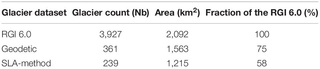
Table 1. Glacier datasets used in the present study, together with their respective cumulative area and the corresponding fraction of the RGI 6.0.

Data and Methods

In order to assess the glacier mass change over the 17 years of the study period, we computed for every selected glacier both the geodetic mass balance corresponding to a multi-decadal average and the annual mass-balance time series from the SLA-method.

Reconstructing Multi-Decadal Mass Balance From Digital Elevation Models

Over our study area, 7306 ASTER DEMs were generated using the Ames Stereo Pipeline (Shean et al., 2016; Beyer et al., 2018). DEMs are co-registered over stable terrain (excluding ice and lakes) following the Nuth and Kääb (2011) approach and using the Global DEM (GDEMv2, Tachikawa et al., 2011) as a reference. Following Berthier et al. (2016), for each 30 m pixel, a two-step linear regression is fitted to the ASTER-derived DEMs to estimate the temporal trend in elevation change (dh/dt). The overall dh/dt for each considered individual glacier is derived using the RGI 6.0 outlines (RGI Consortium, 2017). These outlines are also used to separate glacierized and ice-free terrain and to average dh/dt for individual glaciers. Data gaps are filled using the local hypsometric approach (McNabb et al., 2019).

In order to estimate the decadal glacier-wide mass balance, surface elevation changes are converted into mass changes by applying the volume-to-mass conversion of 850 ± 60 kg.m^–3 (Huss, 2013).

Although the ASTER geodetic mass balance method has its limitations (mostly related to the spatial resolution of the DEMs), it also has the prominent advantage to make possible regional applications, as demonstrated by several recent studies (e.g., Brun et al., 2017; Menounos et al., 2019; Dussaillant et al., 2019; Shean et al., 2020). Far less glaciers are covered by existing high resolution DEMs in the European Alps, and those are restricted to specific time periods. Quality assessment of the ASTER method in comparison with high resolution DEM-differencing has been performed over the Mont-Blanc range by Berthier et al. (2016) using SPOT5 and Pléiades DEMs, or for glaciers in British Columbia by Menounos et al. (2019) using LiDAR DEMs. Both studies concluded that there was an absence of bias using ASTER and a very good agreement between the geodetic mass balances quantified for individual glaciers down to 0.5 km² in area.

Reconstructing Annual Surface Mass Balance Time Series From Optical Satellite Images

The geodetic approach provides spatially-resolved mass balance estimation over decadal time spans, but is currently unable to resolve the annual fluctuations for mountain glaciers. To derive the annual surface mass balance using the SLA-method, the first step consists of estimating the SLA. Because of the large number of glaciers considered in this study, we semi-automatically identified the transient snowline altitude using the algorithm detailed in Supplementary Material. We used images of decametric resolution from optical satellite sensors (i.e., LANDSAT 5, 7, 8, Sentinel-2, ASTER) and identified the transient SLA using a band ratio NIR²/SWIR to enhance the snow/ice contrast. The ASTER GDEM v2 was used to compute the snowline altitude. To avoid side effects on the glacier (e.g., shadows from the surrounding rock faces, avalanche deposits), transient SLAs were derived on a central part of the glacier. For each image, the algorithm allows detection of the glacier’s transient SLA as the steepest gradient in the surface band ratio signature, corresponding to the local transition between ice and snow. For each glacier and each year, we then considered the highest transient SLA to be representative of the glacier’s annual SLA. For a given glacier, when the time series of annual SLAs contained gaps, for example those due to cloud cover or image unavailability, we used the statistical linear approach of Lliboutry (1974) for gap-filling. This approach takes into account inter-annual (regional effect, according to neighboring glaciers from the surrounding region) and spatial (site effect, according to the average of each individual glacier) variability to reconstruct missing annual SLAs values in the time series. Glaciers for which the time series of annual SLAs contains more than 68.2% (1σ) of missing data were discarded leading to the number of 239 glaciers monitored. To define the neighboring glaciers used in the gap-filling approach, we followed the conclusion by Vincent et al. (2017) and Pelto (2018) that showed that glaciers 100 km apart have a significant common variance (75% in the European Alps for surface mass balance data, Vincent et al., 2017). As the SLA is a good proxy of the mass balance, we assumed that the same relationship applies, with neighboring glaciers (100 km apart) having coherent migration of the SLA from one year to another.

Using the SLA-method presented in Rabatel et al. (2005, 2008, 2016, 2017), the glacier-wide annual mass balance has been reconstructed for the period from 2000 to 2016. In summary, with this method, the cumulative mass loss of the glacier over the study period (the average annual mass balance rate, $\stackrel{.}{M}$, in m w.e. yr^–1) is given by the geodetic method. On the other hand, the annual glacier-wide mass change (M_i, in m w.e.) for every year i of the study period results from the difference between altitude of the snowline at the end of the ablation season (SLA_i, in m a.s.l.) and the theoretical altitude of the equilibrium line if the glacier had a balanced budget (glacier wide mass balance = 0) over the study period (ELA_eq, in m a.s.l.), multiplied by the mass-balance gradient (∂b/∂z) in the vicinity of the ELA.

Therefore, assuming that SLAs are approximations of ELAs, ELA_eq is computed as:

and M_i is computed as:

Regarding ∂b/∂z, it may vary from one glacier to another due to local influences on the meteorological conditions that govern accumulation and ablation patterns, and also from one year to another considering any single glacier (e.g., Kuhn, 1984; Mayo, 1984; Benn and Lehmkuhl, 2000; Rabatel et al., 2005). For instance, on the basis of the three glaciers in the French Alps, Rabatel et al. (2005) quantified a coefficient of variation of the mass balance gradient of 30%. However, several studies demonstrated that choosing a regional ∂b/∂z does not depreciate the results and leads to similar results that individual glacier ∂b/∂z estimates (Rabatel et al., 2005, 2016; Chandrasekharan et al., 2018). This underlines the low sensitivity of the SLA-method to the ∂b/∂z value, which allows using the SLA-method on unmonitored glaciers and avoiding calibration. It is noteworthy that Braithwaite (1984) already mentioned that the value of what he called the “effective balance gradient” was not the main source of error, but rather the value of the “balanced-budget ELA” (called ELA_eq in our case). We therefore selected a mass-balance gradient of 0.0078 m w.e. m^–1 according to Rabatel et al. (2005) and assumed its validity at the scale of the European Alps, considering an uncertainty of ± 30% to take into account its spatio-temporal variability.

Uncertainty in the Annual and Decadal Retrieved Glacier-Wide Mass Balance

The uncertainty in multi-decadal geodetic mass balance of individual glaciers is related to three independent sources: the uncertainty in the glacier area, the uncertainty in dh/dt, and the uncertainty in the volume-to-mass conversion factor. The uncertainty in the rate of elevation change integrated over the area of each glacier is estimated following Rolstad et al. (2009) with a 500 m range spherical variogram (Menounos et al., 2019). The standard deviation of dh/dt over stable terrain is computed in 1 × 1 degree tiles and applied to glaciers in the corresponding tile, with an average value of 0.5 m yr^–1. The uncertainty in the glacier surface area is conservatively defined as 5% for clean-ice glaciers (Paul et al., 2013), and the uncertainty in the volume-to-mass conversion factor is estimated as ± 60 kg m^–3 (Huss, 2013). We considered these uncertainties to be applicable on the very few glaciers that have a covered glacier tongue in our sample. The geodetic mass balance uncertainty is estimated for each glacier, with a mean value of ± 0.16 m w.e. yr^–1, ranging from ± 0.06 to ± 0.83 m w.e. yr^–1 for the 361 glaciers monitored with the geodetic method.

The overall uncertainty in the retrieved annual mass change is due to the propagation of the uncertainty of each variable used in the calculation (Equations 1 and 2). It therefore corresponds to the quadratic sum of:

• The uncertainty in the semi-automatically retrieved SLA, equal to ± 123 m. It takes into account: (i) the DEM resolution and uncertainty; (ii) the pixel size and resampling of the satellite images used for the detection; (iii) uncertainties related to the detection method and potential false detections caused by the presence of a firn line, the presence of crevasses, undetected clouds or changes of slope not mitigated by the algorithm; and (iv) uncertainties related to the gap-filling approach. A full description is presented in Supplementary Material.

• The uncertainty related to ∂b/∂z in the vicinity of the ELA, considered as ± 30% of ∂b/∂z as suggested by Rabatel et al. (2005).

• The uncertainty in the computed geodetic mass balance presented above.

• The time difference between the image acquisition used to estimate SLA, and the last day of the hydrological year. Rabatel et al. (2016) estimated this uncertainty at ± 0.09 m w.e. yr^–1 in average on 30 glaciers in the French Alps for a 30 years study period. This estimate made for glaciers in the French Alps is assumed to be valid at the scale of the European Alps.

The uncertainty in the computed annual mass balance of the 239 glaciers monitored with the SLA-method equals ± 0.52 m w.e. on average, ranging from ± 0.49 to ± 0.60 m w.e. depending on the year and the glacier. It should be noted that the uncertainty in the annual mass balance can be assumed to be higher for small glaciers (because of a higher signal/noise ratio in the dh/dt maps used for the geodetic mass balance) or for steep glaciers (because of a higher uncertainty in the SLA estimate) or for years with fewer images. If the first two sources are considered in our uncertainty estimate, it is much more difficult for the third point as it depends on the year considered and the meteorological conditions during the summer seasons. Indeed, for a given year, one single image might be available, but if recorded at the good moment of the summer season, the SLA estimate will be accurate. On the contrary, the retrieved SLA will likely be considered as an outlier and be removed by the post-processing steps of the workflow (see section 1.2.2.10 in Supplementary Material).

Finally, one must keep in mind that a good way to validate the method is the comparison between the retrieved annual mass balance time series with the ones quantified from field measurements where such data are available (see below, section Remotely-Sensed SLA and Annual Mass Balance Validation).

Climatological Data

In order to evaluate the role of climate forcing on the observed glacier mass changes, we analyzed the climatic conditions during the period from 1984 to 2016 using data from the ERA5 reanalysis (Copernicus Climate Change Service [C3S], 2017). The reason for doubling the time window is to study the climatic trends over a sufficient time span (conform to the standard of 30 years). Direct links with the computed annual mass balance were performed on the same period (2000–2016). We used ERA5, a global atmospheric reanalysis produced by the European Centre for Medium-Range Weather Forecasts (ECMWF), at a horizontal resolution of 30 km and on 137 vertical levels, currently starting in 1979. Atmospheric reanalyses accommodate conventional and satellite observations within the physically consistent framework of a numerical prediction model. ERA5 is the state-of-the-art global reanalysis. In this study we analyzed glacier-relevant variables from ERA5 such as 2 m air temperature, precipitation, sea-level pressure, wind speed at 700 hPa, precipitable water, moisture, and heat transport. To analyze predominant climatic factors on the computed annual mass balance, we performed principal component analysis (Wilks, 2011) on these variables.

Results

Remotely-Sensed SLA and Annual Mass Balance Validation

Taking advantage of manually derived SLA for 34 glaciers in the western Alps (Rabatel et al., 2013, 2016), we were able to validate our semi-automatic estimates of SLA (displayed Figure 1A, further assessments in Supplementary Material). Overall, our estimates are largely able to reproduce manual estimations of the annual glacier SLA (r² = 0.41 for 506 compared SLA, significant at the 1% risk level), with a mean observed bias of + 35 m. Despite the filtering and gap-filling post-treatment, discrepancies persist (RMSE = 144 m). Those discrepancies can arise from the date differences between both estimates, the different SLA detection zone (central part of the glacier vs. full glacier width for the manual estimates), or errors inherent to the SLA detection. Our estimated uncertainty in the semi-automatically derived SLA (± 123 m), although slightly smaller than the computed RMSE, accounts for these sources of errors when estimating the annual SLA and the associated annual mass balance.

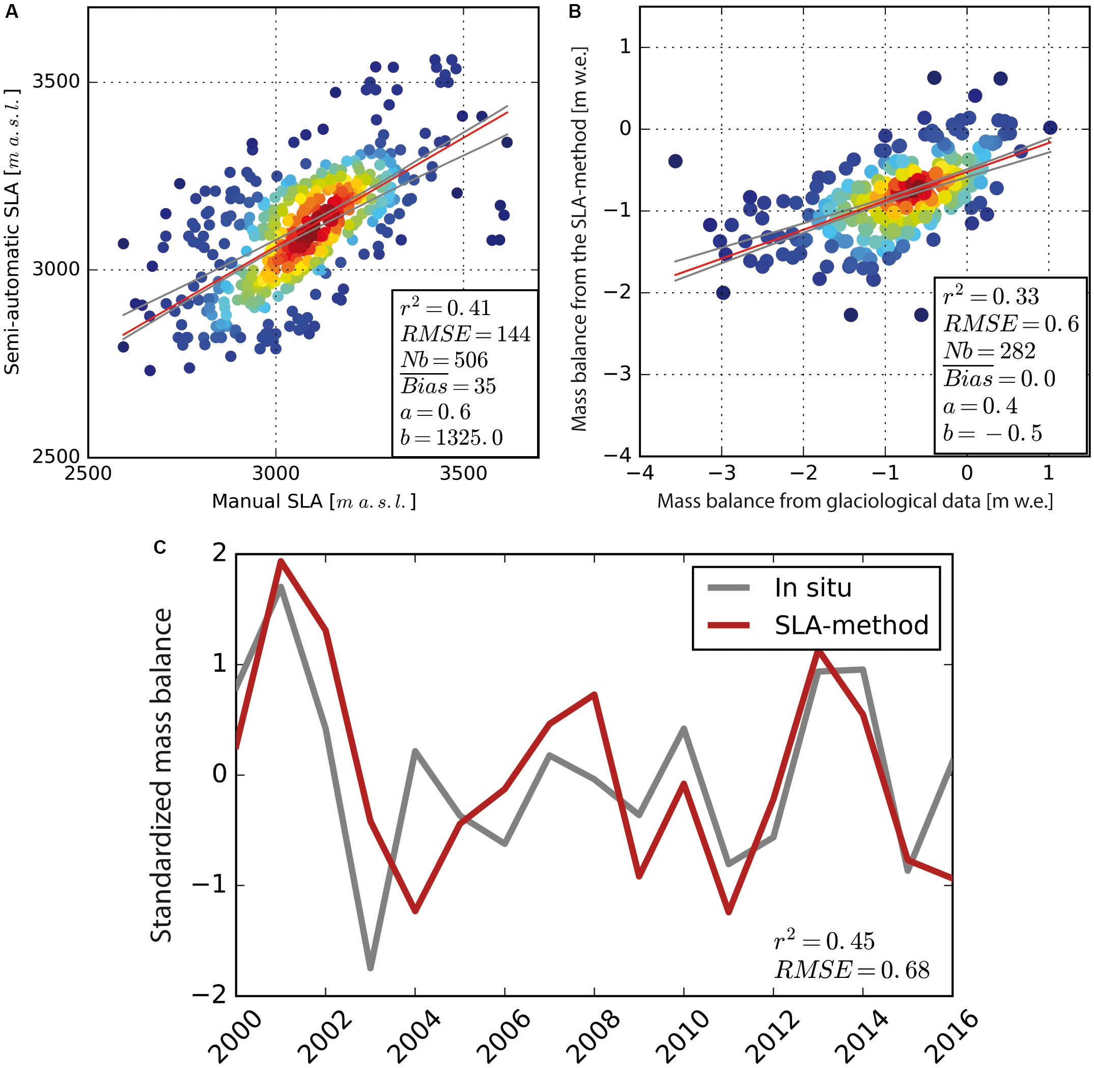
Figure 1. (A) Illustrates the comparison for filtered and gap-filled SLA on 34 glaciers in the western Alps (506 compared SLA). (B) Illustrates the comparison between mass balances computed with the SLA-method vs. annual mass balances from the glaciological method on 23 glaciers (282 compared annual values). Error bars are not shown in (A,B) for better readability; refer to the text for their ranges. In (C), the mean standardized interannual variability is represented for in situ and SLA-method estimates for the 23 glaciers monitored in situ and detailed in Supplementary Table S3. For (A,B), the red line indicates a robust linear regression with support for the M-estimators (Susanti et al., 2014), together with the 95% confidence interval, materialized by the gray lines. Heat-map style colors are an indicator of the point density with one point representing one glacier and one year. For (A–C), statistics are displayed to assess the correlation between both datasets; a represents the slope of the linear regression and b the intercept.

Using the SLA-method, we reconstructed glacier-wide annual mass balance time series for the period from 2000 to 2016. The European Alps being one of the most monitored glacierized regions worldwide, we were able to validate our estimates by comparing to 23 glacier-wide annual mass balance time series estimated with the glaciological method (full list and time series length are presented in Supplementary Table S3). As displayed in Figure 1B, annual mass balance from the SLA-method and from in situ data are in general agreement, with 33% of common variance, no observed mean bias, and a RMSE (0.6 m w.e. yr^–1) slightly larger than the uncertainty for SLA-method mass balances (± 0.52 m w.e. yr^–1 in average). There is an underestimation for highly negative annual mass balances (and to a lesser extent for very positive ones), resulting in the slope of the linear regression being equal to 0.4 rather than 1. In Figure 1C, we compare the standardized glacier-wide annual mass-balance time series (average of the 23 glaciers monitored in situ) quantified from in situ and SLA-method estimates. Standardized values are calculated as described by Equation S4 in Supplementary Material replacing SLA by mass balance. One can note the overall good agreement between the two-time series in terms of interannual variability (r² = 0.45), except between 2004 and 2008. There are several possible explanations for the remaining discrepancies:

• Errors in SLA estimation,

• Lack of representativeness of the computed glacier-wide mass-balances from sparse in situ data,

• Difference of glacier extent used to compute the glacier-wide mass balance in the two methods,

• Errors and/or difference between geodetic estimates used to constrain glacier-wide annual mass balance.

Indeed, when comparing manually delineated and semi-automatically derived SLA (Figure 1A and section 1.3.1 and 1.3.2 in Supplementary Material), the algorithm fails to reproduce extremely high or sometimes very low SLA due to the position of the SLA itself, either too close to the glacier head or snout. Therefore, retrieved mass balances from the SLA method do not capture extreme years (mainly the most negative ones) as well as others, explaining part of the observed discrepancy. Furthermore, most of the SLA estimates between 2003 and 2008 were based on Landsat 7 images, for which the Scan Line Corrector (SLC) failed in May 2003, resulting in stripped images and thus reducing drastically the number of usable images to detect the SLA. On the other hand, glacier-wide estimates from in situ data using the glaciological method are dependent on the point measurements distribution on the glacier (often biased toward the ablation area due to access facilities), on the interpolation method, and on glacier area changes during the monitored period (e.g., Thibert et al., 2008). Geodetic calibrations can reduce the related errors when photogrammetry acquisitions are performed (Zemp et al., 2013). In addition, in situ glacier wide mass balances can show surprising values, such as exhibited by the north-facing Corbassière Glacier in 2006, with a measured annual surface mass balance of −3.56 m w.e. and a corresponding ELA at 3,875 m a.s.l., which is more than 450 m above the uppermost manually delineated SLA from neighboring French glaciers for the period 1984–2010 (Rabatel et al., 2013). Such negative surface mass balance values from in situ measurements are questionable and can be a potential source of discrepancy with the SLA-method estimates. Finally, the dissimilar glacier surface areas considered in the two methods could explain part of the differences. Indeed, glacier surface areas used for the SLA and geodetic methods correspond mostly to glacier outlines delineated around 2003 in the European Alps (RGI Consortium, 2017), while the year of delineation used in the glaciological method varies from glacier to glacier and can depend on local inventories. Applying the same methodology than we used to derive geodetic mass balance for the Andean glaciers over a similar time period, Dussaillant et al. (2019) estimated that considering a single or multiple inventories could lead to a difference of mass balance rate up to 10% for individual fast retreating glaciers, but of only a few% for glacier larger than 3 km² (see section 7 of Supplementary Information of their paper).

Despite the observed discrepancies, the annual mass balances computed from the SLA-method are able to reproduce the monitored surface mass balance from in situ measurements together with the interannual variability (Figures 1B,C). Therefore, this justifies the application of the SLA-method at a regional scale, and underlines the ability of the method to: (i) reconstruct the annual mass-balance time series; (ii) investigate the behavior of the glaciers for the different regions; and (iii) observe the annual variability for inaccessible glaciers.

Regional Mass Balance Over the European Alps

Multi-decadal mass balances and annual mass-balance time series averaged by sub-regions are presented in Figures 2, 3, respectively. According to Figure 2, the sub-region #4 (Eastern Berner and Urner ranges) experienced the strongest mass loss between 2000 and 2016, with an average of −0.90 ± 0.20 m w.e. yr^–1. On the other hand, the sub-region #1 (North of Ötztaler, Stubai, and Zillertal ranges) experienced the least negative mass balance, with −0.54 ± 0.28 m w.e. yr^–1 on average. The length of the ASTER images archive gives the opportunity to divide the study period (2000–2016) into two sub-periods (2000–2009 and 2009–2016), as was done in the study by Menounos et al. (2019) and Dussaillant et al. (2019), although no contrasted pattern was observed between the two. The multi-decadal mass balance for the European Alps over the period from 2000 to 2016 is −0.74 ± 0.20 m w.e. yr^–1, corresponding to an average annual loss of −1.54 ± 0.38 Gt. Over the same period, Zemp et al. (2019) computed a region-wide mass balance of −0.83 ± 0.07 m w.e. yr^–1 for glaciers of the European Alps. Our estimate is lower even if the values are not statistically different considering the uncertainties. Because Zemp et al. (2019) computed their region-wide mass balance by combining the temporal variability from in situ measurements with geodetic estimates different from ours, the discrepancy with our region-wide mass balance is therefore also related to the used methods and data.

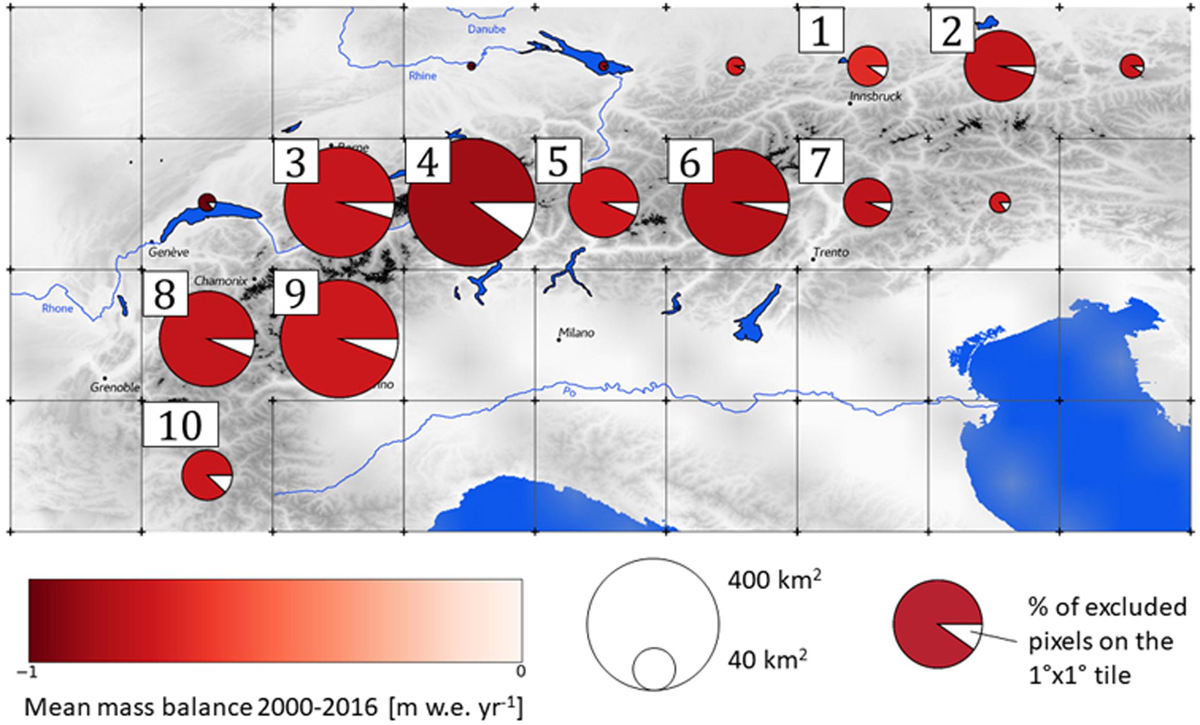
Figure 2. Map of the European Alps illustrating the glacierized and the ice-free (thin black frames) 1 × 1 degree grid cells. For each glacierized cell, the pie charts illustrate the mean mass balance from 2000 to 2016 computed with the geodetic method, with white slices corresponding to the percentage of outliers removed during the filtering of the dh/dt maps within each tiles. Numbers (1–10) denominate regions where annual mass balance time series have been computed using the SLA-method.

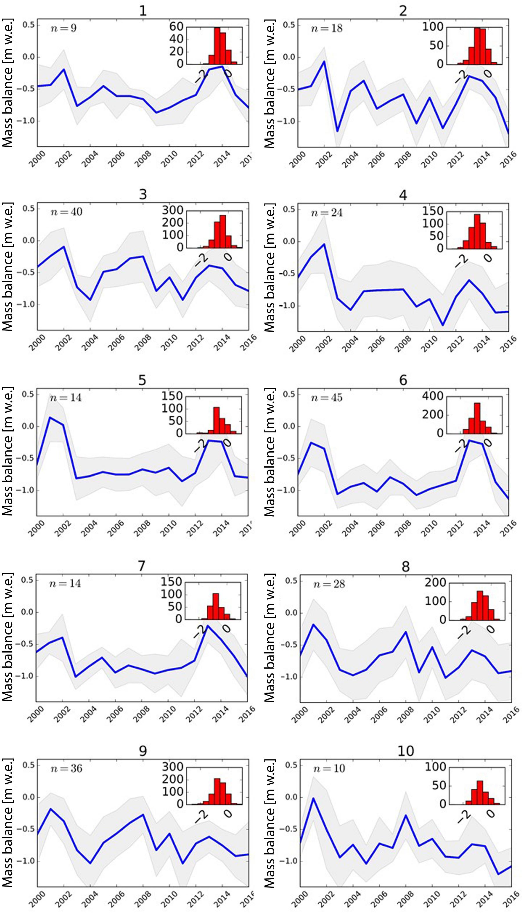
Figure 3. Mean annual mass balance time series (in m w.e.) for each of the ten studied sub-regions (defined in Figure 2). The gray shade illustrates the annual dispersion of the mass balance estimates for individual glaciers in the sub-region, computed using the standard deviation at 1σ. The number of glaciers (n) is given on the top-left corner of each subplot. The red histograms present the statistical distribution of annual mass balances as a function of its value, in m w.e.

Regarding the interannual variability of the annual mass-balance time series, contrasted patterns can be observed from one region to another, as displayed in Figure 3. The easternmost and westernmost sub-regions (respectively, sub-regions #2 and #3, #8, #9, #10) show a high temporal variability from one year to another. For the central part of the European Alps (sub-regions #1, #4, #5, #6 and #7), the interannual variability in the computed mass balance is less pronounced from 2003 to 2012, experiencing almost constant mass balance (between −0.5 and −1 m w.e. yr^–1, function of the sub-region). Peculiar events can be observed across the entire range, during 2001–2002 and 2013–2014 for low losses and 2003 and 2004 for high losses years. These results are discussed in relation to the variability of climatic variables in section Analysis of Climatic Drivers below.

Glacier Morpho-Topographic Features, One of the Multi-Decadal Mass Balance Drivers?

Previous studies showed that multi-decadal mass balances of individual glaciers can be related to glacier morpho-topography (e.g., Paul and Haeberli, 2008; Rabatel et al., 2013, 2016; Fischer et al., 2015; Brun et al., 2019). In addition, according to Vincent (2002); Abermann et al. (2011), or Huss (2012), differences in specific mass balance between neighboring glaciers can often be controlled more by glacier morpho-topography than by climate variability, and observed mass balance response to similar climate forcing can largely differ from one glacier to another (e.g., factor of four in terms of cumulative mass losses between Silvretta and Sarennes glacier, Vincent et al., 2017). However, assessing the impact of glacier morpho-topography on the average glacier mass balance is challenging due to the limited number of in situ measurements, which are not necessarily representative of the diversity of glaciers within the same region (Gardner et al., 2013). Therefore, geodetic estimates of multi-decadal mass changes for individual glaciers at regional scale provide a lever to investigate the impact of glacier geometry on the decadal mass balance variability from one glacier to another. We tested the relationship between the geodetic multi-decadal mass balance for 361 glaciers for the period from 2000 to 2016, and several glacier morpho-topographic features (i.e., mean glacier slope, minimum, median and maximum altitude, aspect, and area, displayed in Figure 4).

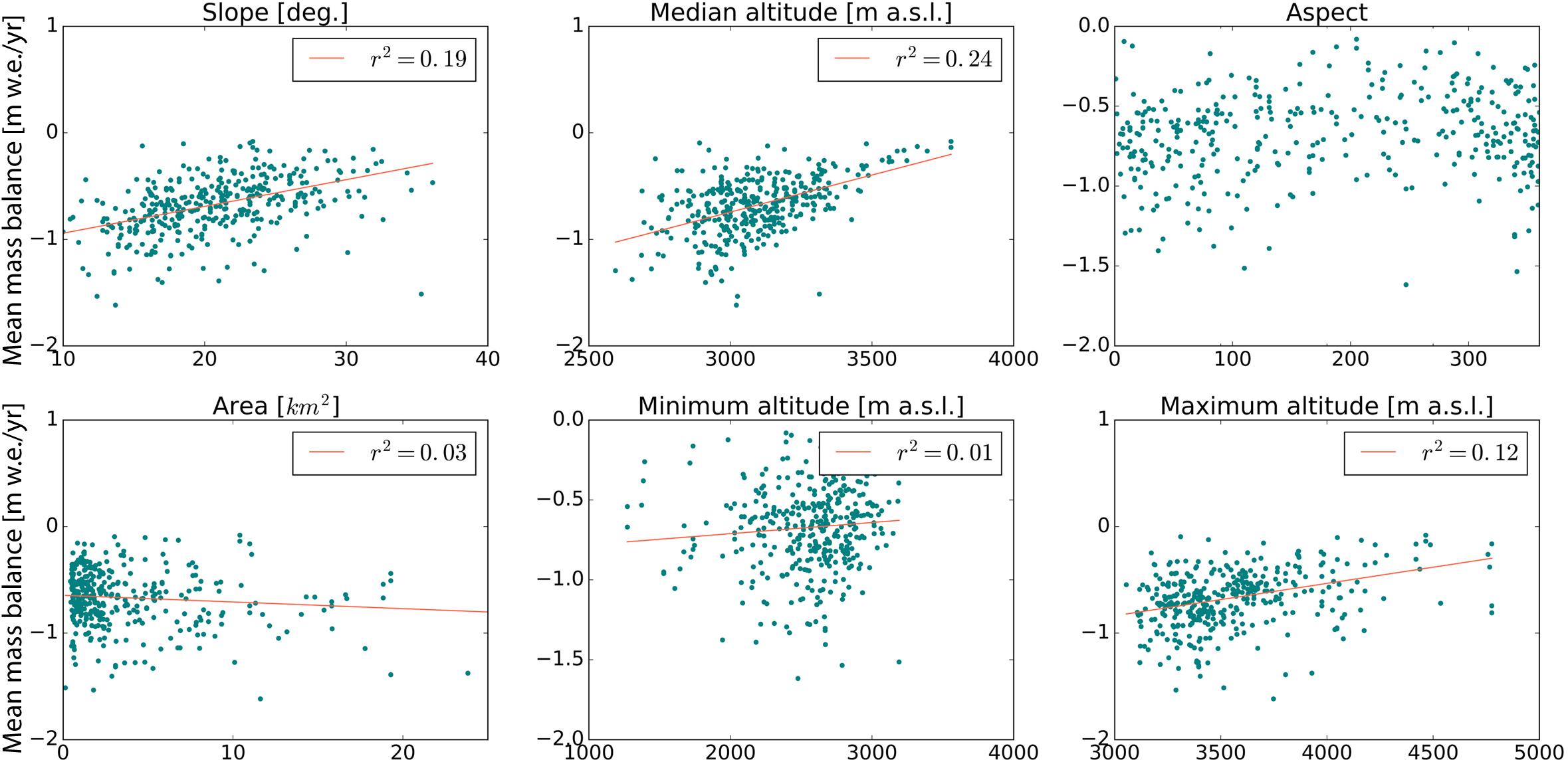
Figure 4. Geodetic multi-decadal average mass balance for the period from 2000 to 2016 as a function of six morpho-topographic variables. A correlation coefficient is provided for each of the variables. A regression has been computed following a robust linear model with support for the M-estimators (Susanti et al., 2014), and is represented by a red line, excepted for the glacier aspect, for which a linear regression was not relevant.

We computed the mean glacier slope on purpose rather than the largely used glacier tongue slope to also take into account accumulation basin geometries. Out of the six features studied, three can be significantly correlated to the multi-decadal mass balance (with a statistical confidence level > 95% according to a Student’s t-test): the median altitude (r² = 0.24), the mean glacier slope (r² = 0.19), and the maximum altitude (r² = 0.12). Using a least absolute shrinkage and selection operator (LASSO) regression analysis, the slope and the median altitude, being the dominant terms, explain 36% of the variance of the observed geodetic multi-decadal mass balance. Adding other variables (area, maximum and minimum altitude, and mean aspect) only raises the explained variance to 39%, which shows their relatively low control on the multi-decadal mass balance at regional scale. This result strengthens previous analyses made in the European Alps (e.g., Huss, 2012; Fischer et al., 2015; Rabatel et al., 2016) and in other mountain regions (e.g., Brun et al., 2019), even if we did not find a significant statistical correlation between the glacier area and the multi-decadal mass balance as in previous work (Paul and Haeberli, 2008; Huss, 2012). This difference could rest on the absence of small glaciers (<0.5 km²) in our dataset.

It is finally worth noting that correlations are positive for the three significantly correlated morpho-topographic variables, suggesting that steep and high glaciers with a high accumulation basin experience the least negative multi-decadal mass balances.

Discussion

Analysis of Climatic Drivers

Spatio-Temporal Variability of the Annual Glacier-Wide Mass Balance Time Series

Rabatel et al. (2013) analyzed the spatio-temporal variability of the ELA in the western Alps using a 25 years time series for 43 glaciers and concluded that the temporal variability of the reconstructed time series is mainly related to the climatic drivers, and the morpho-topographic factors mostly control the average ELA over the study period. Following these statements and assuming they apply to the annual glacier-wide mass balance, we analyzed the spatio-temporal variability of the reconstructed annual mass-balance time series considering different climatic variables commonly used in multiple regression studies on glacier mass balance (e.g., Hoinkes, 1968; Martin, 1974; Braithwaite and Zhang, 2000; Bolibar et al., 2020). As such, for each sub-region (1 × 1 degree grid cell), we computed from ERA5 data: the summer average of the 2 m air temperature (T2ms) and sea-level pressure (SLPs), the zonal and meridian temperature advection (Tus and Tvs), the winter average of precipitation (Pw) and sea level pressure (SLPw), the precipitable water over the entire atmospheric column (Pwatw), and the zonal and meridional humidity advection (Quw and Qvw). We then performed, for each sub-region, a LASSO regression analysis between these climatic variables and the median annual mass-balance time series over the 2000 to 2016 period. For each sub-region, a maximum of three variables explaining most of the observed variance are identified and reported in Table 2. It is worth noting that this statistical analysis is conducted over a 17 years time period, which is rather short from a climate point of view. Therefore, the interpretation of the results has to be considered with caution and as a preliminary study of the relationship between the mass balance and climate inter-annual variability at the European Alps scale.

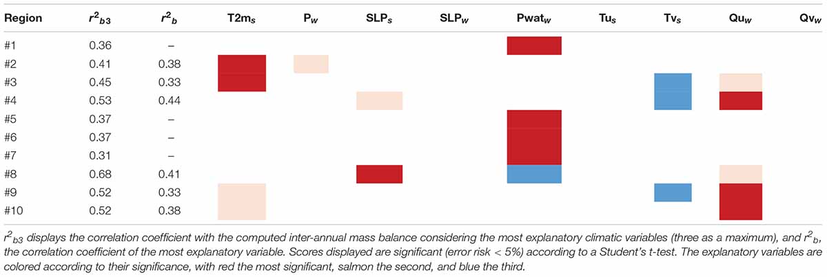
Table 2. Results from multi-linear LASSO regression analysis in between the median annual mass balance and nine climatic variables from ERA5 for each sub-region of the study area.

Interestingly, from the LASSO analysis, the two groups of sub-regions identified from the annual mass-balance time series also emerge. For the sub-regions #1, #5, #6, and #7, the only climatic variable statistically significant and explaining more than 30% of the observed inter-annual mass balance variance is the precipitable water during winter, which is largely impacted by the winter air temperature (maximum water content in humid air depending on temperature). This is in agreement with observations made for glaciers in these regions (i.e., Austrian Alps, Abermann et al., 2011) suggesting that glaciers in this area could be maintained because of “above-average accumulation.”

Sub-regions #3, #4, #9, and #10 have the same first explicative variable (Quw, except for #3 and #8 where it is second), corresponding to eastward advection of humidity and seems also highly impacted by summer air temperature and summer meteorological conditions (Tvs, SLPs, and T2ms), mainly dominated by southward fluxes. These sub-regions are all in the western European Alps and could therefore experience similar meteorological forcing during zonal or meridian meteorological events.

Sub-region #2 seems to be highly impacted by summer meteorological conditions and could not be assimilated to any other sub-region. Contrary to sub-region #3, #2 does not seem impacted by temperature or humidity advection and is too distant from #3 to be grouped with, despite their common high dependence to summer air temperature. Finally, the sub-region #8 is dominated by summer meteorological conditions, winter eastward humidity advection, and precipitable water. The predominating drivers and observed inter-annual mass balances are not identical from the surrounding regions despite their close geographical distances, and our analysis does not allow concluding on the reasons for this peculiar behavior.

Surprisingly, winter precipitation is not identified as an explanatory variable for any of the monitored regions. One hypothesis could rest on the poor capacity of ERA5 to spatialize precipitation regarding the relatively low resolution of the used DEM (i.e., 30 km), particularly important in mountainous terrain. Precipitable water is often considered as a more accurate variable as it does not provide a spatial estimation of precipitation but rather a budget of precipitable water.

Climatic Patterns for Extreme Years

Our results also allow analyzing peculiar years such as the most/least negative one (Figure 5A) and relate them to climate forcings. On a year to year basis, the regional mass-balance variability during high loss years is dominated by a pattern which is common to the entire Alpine range (80% of variance explained, Figure 5B). This uniformity was already observed when comparing annual mass balance between each of the ten sub-regions for certain years (Figure 3, section Regional Mass Balance Over the European Alps). We used a principal component analysis to define years of high loss (PC1 < σ/2: 2003, 2004, 2009, 2011) and years of low loss (i.e., positive anomalies, PC1 > σ/2: 2001, 2002, 2013, 2014). The composites of the 700 hPa wind anomalies yield approximately opposite in either case and between winter and summer. During low loss years, the main atmospheric flow is westerly in winter, advecting moist air from the Atlantic (blue arrows, Figure 5C). Conversely, the easterly flow during high loss years is less favorable to precipitation with potentially colder and drier climate conditions. The composites of 500 hPa geopotential height for low and high mass loss years correspond to the positive and negative phases of the North Atlantic Oscillation in the winter weather regime classification of Cassou et al. (2004). In summer, the wind is easterly during low mass loss years and westerly during high mass loss years (blue arrows in Figure 5D). The associated 500 hPa fields match the “Blocking” and “Atlantic low” patterns, respectively (Cassou et al., 2005).

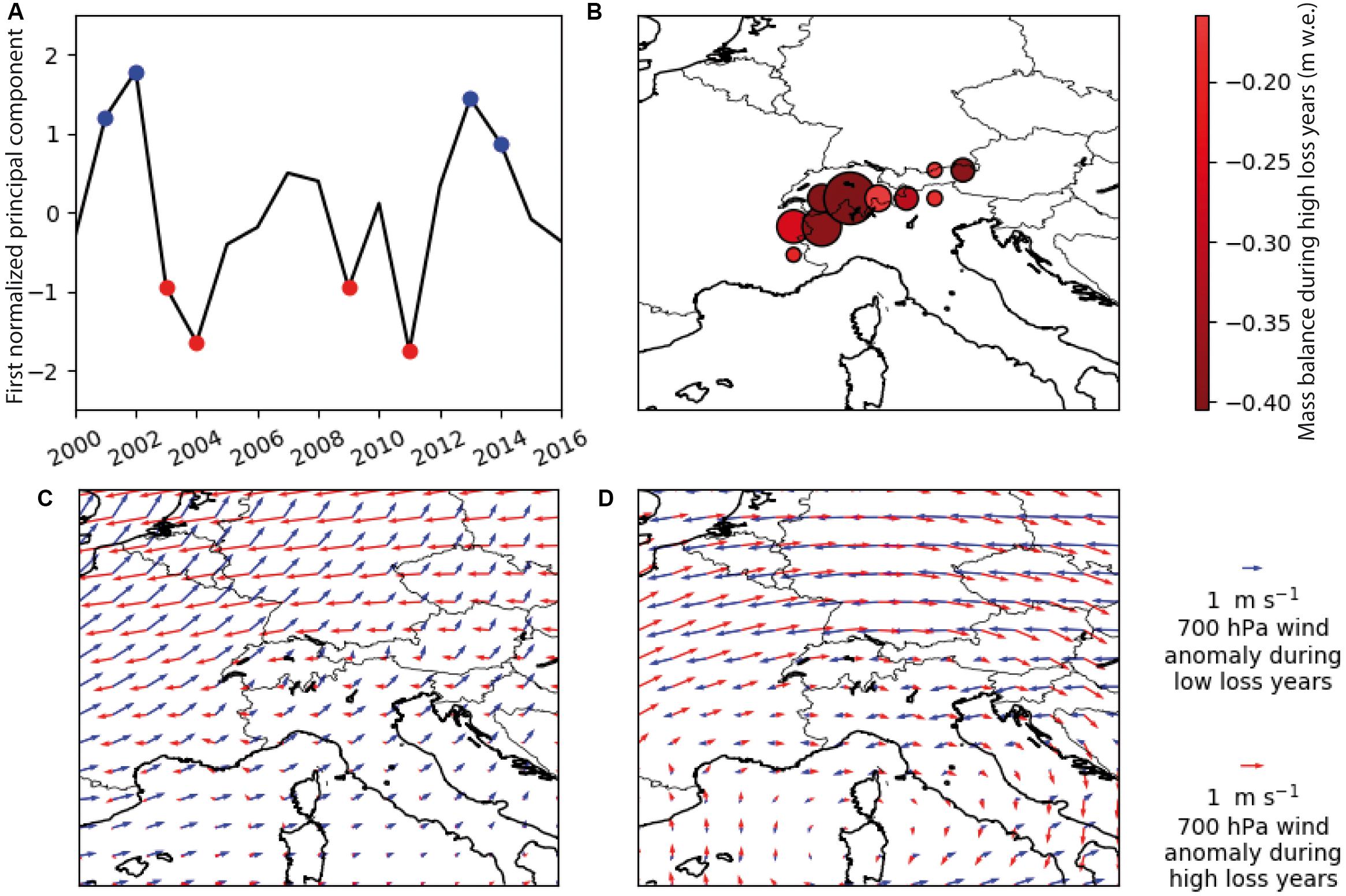
Figure 5. Time series of the normalized first principal component of annual regional mass balances (A), composite of annual regional mass balances during high loss years (B), 700 hPa composites during high and low loss years (red and blue arrows) in winter (C) and summer (D).

The second principal component opposes East to West in terms of interannual mass-balance patterns, with the boundary falling between regions #3 and #4. This pattern could also be observed visually on Figure 3, with regions #1, #5, #6, and #7 experiencing sustained mass losses from 2003 to 2012, while Western regions experience more interannual variability. However, the second principal component accounts for only 7% of the variance and could not be related to a straightforward atmospheric mechanism.

Attribution of Today’s Glaciers’ Mass Loss in the European Alps

According to the ERA5 reanalysis, summer temperature shows an overall increase over the entire region, ranging from + 0.4 to + 0.8K from 1984 to 2016 (significant at the 5% level). For winter precipitation, changes are not statistically significant. Interestingly, the 2000–2016 period we studied here is characterized by important glacier mass losses in the European Alps (−0.74 ± 0.20 m w.e. yr^–1 in average from our findings) which can be mainly attributed to high melting compared with the period from 1960 to 1990, when glaciers experienced very limited mass losses (e.g., Beniston et al., 2018; Zemp et al., 2019). Considering Braithwaite and Zhang’s (2000) findings that showed a sensitivity of glacier wide mass balance of −0.77 m w.e. a^–1°C^–1 for five glaciers in the Swiss Alps, we can state that the strong glacier imbalance currently experienced by glaciers in the European Alps is likely mainly the result of the atmospheric temperature increase that can be observed in the ERA5 data.

Representativeness of in situ Monitored Mass Change

Historically, glacier-wide mass change was monitored in situ and glaciers have often been chosen because of their access, their morpho-topographic features enabling their instrumentation, or for political and historical reasons (Kaser et al., 2003). The “ideal” glacier for mass balance investigation does not represent the global glacier diversity, which may lead to biases if such a glacier is considered as representative of the regional scale glacier behavior. Indeed, negative biases have already been observed when comparing region-wide mass balance estimations using laser altimetry to interpolations of sparse glaciological measurements (Gardner et al., 2013). Recently developed geodetic methods help overcoming this issue of representativeness due to higher temporal and spatial resolutions of the computed mass balances (e.g., Menounos et al., 2019; Zemp et al., 2019).

To see whether the in situ monitored glaciers in the European Alps are representative of the regional behavior, we analyzed the cumulative mass balance of the 239 glaciers in the European Alps for which annual mass-balance time series have been computed, as a function of the glacier morpho-topographic features, such as mean glacier slope, median and maximum altitude (significantly correlated to the average glacier wide mass balance, see section Glacier Morpho-Topographic Features, one of the Multi-Decadal Mass Balance Drivers?). Figure 6 illustrates the cumulative mass balance from 239 glaciers computed from the SLA-method divided into glacier slope quartiles, and the average of the 23 mass balance time series obtained with the in situ glaciological method.

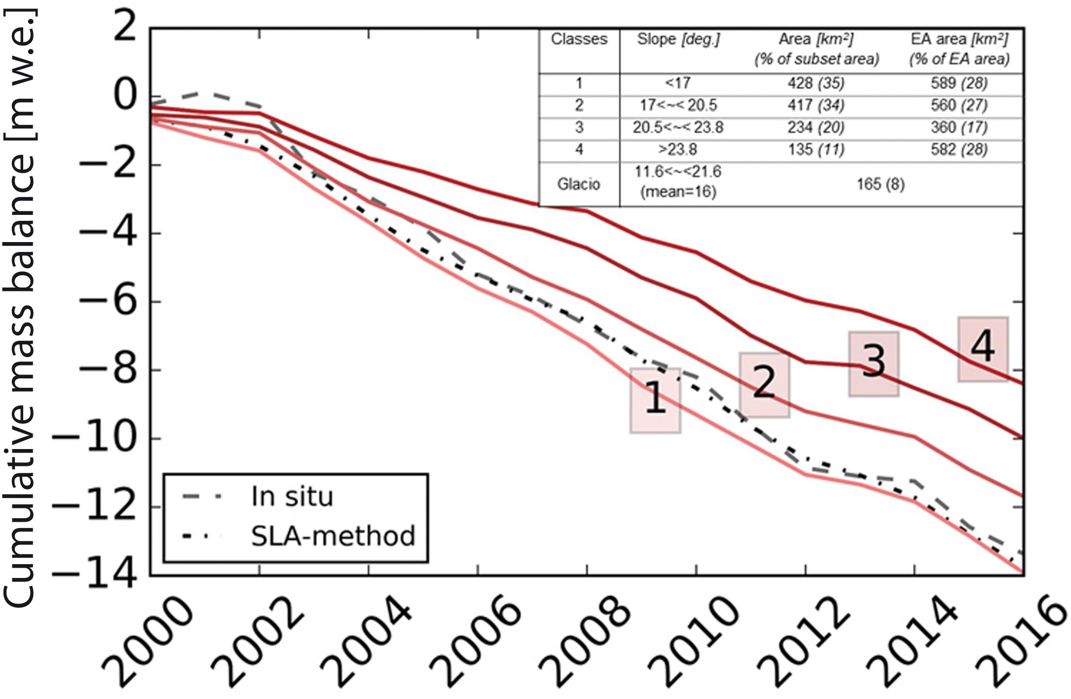
Figure 6. Cumulative mass balance of glaciers from the European Alps vs. their mean slopes. The dashed lines represent the median cumulative mass balance of 23 glaciers obtained from in situ data (gray) and with SLA-method (black). The curves 1, 2, 3, and 4 correspond to the cumulative mass balance of glaciers sorted into quartiles on the basis of their mean slope. Each class has the same number of glaciers but corresponds to a peculiar total glacier area. The classes’ glacier area of our subset and the corresponding glacier area for the entire European Alps (EA) are displayed in the inset table.

As described in section Remotely-Sensed SLA and Annual Mass Balance Validation, annual mass changes computed with the SLA-method slightly underestimates extremely high and low mass balance values (e.g., a year with positive mass balance in the studied period and 2003, a very low mass balance year in the European Alps). As illustrated in Figure 6, our study period has both positive and negative extremes in the first four years, and the cumulative mass balance quantified from in situ measurements is poorly reproduced by SLA-method for those years. For the rest of the time period, the cumulative mass balance of the SLA-method is able to match the in situ monitored cumulative mass balance. The mean slope of the in situ monitored glaciers (16° ranging from 11.6 to 21.6°) falls into classes 1 and 2 (slopes gentler than 20.5°), and Figure 6 (+ the inset Table herein) shows that the median of the 23 in situ mass balance time series is in agreement with the SLA-method mass balance for glaciers having a similar mean slope. As shown in Figure 4, the gentler the glacier slope, the higher the overall mass loss. This relationship has already been observed, either sporadically on small sets of glaciers (e.g., Huss, 2012; Rabatel et al., 2016), or at a larger scale (e.g., Fischer et al., 2015; Brun et al., 2019). From Figure 6, we can also note that the in situ mass-balance time series fails to represent glaciers from classes 3 and 4 (slope greater than 20.5°), yet these classes account for 45% of the glacierized area of the European Alps. We therefore suggest that in situ mass-balance time series may convey a negatively biased picture of the regional behavior because they under-sample steep glaciers, representing almost half of the glacier coverage in the European Alps.

A similar analysis has been conducted using the glacier median altitude (instead of classes of glacier slope), but the only noteworthy class (with a median altitude greater than 3,207 m a.s.l. vs. 3,103 m a.s.l. in average for in situ monitored glaciers, Supplementary Figure S9) concerns about 20% of the total European Alps’ glacierized area, and glaciers from the glaciological sample are spanning over the four defined classes, not permitting to conclude on significant relationships or mis-representativeness of the glaciological sample. When dividing our glacier sample into classes of maximum altitude, glaciers with higher maximum elevations seem to experience less negative mass balances (see Supplementary Figure S10). It is important to highlight that SLAs are rarely observable at the end of the melt season during high loss years for glaciers with low maximum elevations (<3,100 m a.s.l.). These glaciers were therefore discarded in our study, and our subset is not representative of the total European Alps population (12% in our subset vs. 46% for the entire European Alps, in terms of corresponding area for glaciers with maximum altitude < 3,471 m a.s.l.).

From these analyses and in line with the results presented in section Glacier Morpho-Topographic Features, One of the Multi-Decadal Mass Balance Drivers?, we can mention that glaciers with steep slopes and high maximum elevation experienced lower mass loss over the study period. Possible interpretations are that the mean slope and the mass transfer are related, with steeper glaciers having faster dynamics and, that glaciers with higher accumulation areas (i.e., still having a wide accumulation zone) have lower mass balance sensitivity. This hypothesis would imply that steeper glaciers with wide accumulation area faster reach a balanced-state with less negative mass balances while glaciers with low slope remain imbalanced for a longer time, experiencing more negative mass balances to adapt to changing climatic conditions (corroborated by e.g., Brun et al., 2019; Zekollari et al., 2020).

Conclusion

We quantified a spatially resolved estimate of individual annual mass-balance time series for 239 glaciers in the European Alps, using both geodetic and snowline altitude estimates for the period from 2000 to 2016. Benefiting from in situ mass changes data from 23 glaciers, we were able to validate our approach, which is based on the SLA-method to quantify the annual mass balance of individual glaciers at regional scale. The observed discrepancies with in situ estimates are attributable to both the uncertainties and limitations in the semi-automatic SLA algorithm (e.g., underestimation of very negative mass balance years) and to glacier-wide estimates from in situ surface mass balance.

Geodetic estimates of long-term mass changes were used to analyze the impact of glacier morpho-topographic features on the mass changes. Three morpho-topographic variables – mean glacier slope, median, and maximum altitude – appear to explain 19, 24, and 12%, respectively, of the observed variance of the long-term mass changes. An analysis of the cumulative mass balance from in situ and SLA-method estimates suggests that steeper and higher glaciers experienced reduced mass losses. Our analysis suggests that the mass balance time series from glaciers with in situ measurements are not fully representative of the regional behavior of glaciers in the European Alps. Indeed, these glaciers belong to the “gentle slope glaciers” (<20°), and half of the glaciers in the European Alps with higher slope experienced a lower cumulative mass loss. Nonetheless, in situ measurements still provide essential data (particularly point measurements) for the comprehension and modeling of surface processes and glacier response to climate forcing at fine spatial and temporal scales. They are also essential to validate mass change estimates from different remote-sensing methods.

The broad coverage of the Alpine region allowed our mass change estimates to be analyzed in relation with a global atmospheric dataset, namely the ERA5 reanalysis. The yearly resolution of the mass balance time series allowed the identification of two opposite weather regimes favorable or detrimental to the mass balance depending on the time of the year.

Finally, this study proposes a new methodological framework to quantify the long-term trends and the annual mass-balance time series of individual glaciers at regional scale from optical satellite remote sensing only. It also shows an example of data combination to assess climatic causes of observed regional mass changes. The satisfactory results we obtained should encourage applying this framework to other glacierized regions, for example, on hardly accessible glaciers and in regions with few or no available annual mass-balance time series.

Data Availability Statement

Geodetic mass balance and annual surface mass balance data are provided as Supplementary Material (in CSV format). Additionally, annual ELA are available to the international community through a French data portal THEIA: https://www.theia-land.fr/product/altitude-de-ligne-dequilibre-glaciaire-annuelle/. The ERA 5 reanalysis can be found at https://climate.copernicus.eu/climate-reanalysis.

Author Contributions

LD, AR, and YA developed the method to automatize the detection of the SLA. AR computed and provided the reference dataset of manually derived SLA. LD and AD performed the analysis between glacier mass changes and climate. RH computed the geodetic mass balances for the entire European Alps and for the period from 2000 to 2016. LD and AR led the writing of the manuscript. All co-authors contributed to the manuscript.

Conflict of Interest

The authors declare that the research was conducted in the absence of any commercial or financial relationships that could be construed as a potential conflict of interest.

Funding

This study was conducted in the context of the French glacier observatory GLACIOCLIM (https://glacioclim.osug.fr) and the Labex OSUG@2020 (Investissements d’Avenir – ANR10 LABX56). We acknowledge the Helmholtz-RSF project grant #18-47-06202. This was IORAS contribution to the St. Arg. #0149-2019-0002.

Acknowledgments

We are grateful to the satellite data providers: Copernicus/EU/ESA for Sentinel-2, USGS for Landsat, and JPL/NASA and METI for ASTER. The ERA 5 reanalysis was made available by courtesy of ECMWF/Copernicus. We are also grateful to Etienne Berthier for numerous fruitful discussions, advice, and comments on the present manuscript. We thank Pascal Sirguey for helping the development of the detection algorithm and for developing part of the images’ corrections. We also acknowledge Fabien Maussion for processing the glacier central flow lines, Delphine Six for fruitful discussions on the method and the manuscript, Juliette Blanchet for advice on the statistical approach developed for the snowline detection algorithm, Maxim Lamare for discussions on topographic correction models, Fanny Brun for glaciological discussions, and Jean Pierre Dedieu for his involvement in the development of the SLA-method. Finally, we are grateful to the scientific editor, MZ, and the two reviewers for their careful review of the manuscript and comments used to improve the study.

Supplementary Material

The Supplementary Material for this article can be found online at: https://www.frontiersin.org/articles/10.3389/feart.2020.00149/full#supplementary-material

References

Abermann, J., Kuhn, M., and Fischer, A. (2011). Climatic controls of glacier distribution and glacier changes in Austria. Ann. Glaciol. 52, 83–90. doi: 10.3189/172756411799096222
Beniston, M. (2003). Climatic change in mountain regions: a review of possible impacts. Clim. Change 59, 5–31. doi: 10.1023/A:1024458411589
Beniston, M., Farinotti, D., Stoffel, M., Andreassen, L. M., Coppola, E., Eckert, N., et al. (2018). The European mountain cryosphere: a review of past, current and future issues. Cryosphere 12, 759–794. doi: 10.5194/tc-12-759-2018
Benn, D. I., and Lehmkuhl, F. (2000). Mass balance and equilibrium-line altitudes of glaciers in high-mountain environments. Quat. Int. 6, 15–29. doi: 10.1016/S1040-6182(99)00034-8
Berthier, E., Cabot, V., Vincent, C., and Six, D. (2016). Decadal region-wide and glacier-wide mass balances derived from multi-temporal ASTER satellite digital elevation models. Validation over the Mont-Blanc area. Front. Earth Sci. 4:63. doi: 10.3389/feart.2016.00063
Beyer, R. A., Alexandrov, O., and McMichael, S. (2018). The Ames Stereo Pipeline: NASA’s open source software for deriving and processing terrain data. Earth Space Sci. 5, 537–548. doi: 10.1029/2018EA000409
Bolch, T., Sørensen, L. S., Simonsen, S. B., Mölg, N., Machguth, H., Rastner, P., et al. (2013). Mass loss of Greenland’s glaciers and ice caps 2003–2008 revealed from ICESat laser altimetry data. Geophys. Res. Lett. 40, 875–881. doi: 10.1002/grl.50270
Bolibar, J., Rabatel, A., Gouttevin, I., Galiez, C., Condom, T., and Sauquet, E. (2020). Deep learning applied to glacier evolution modelling. Cryosphere 14, 565–584. doi: 10.5194/tc-14-565-2020
Braithwaite, R. J. (1984). Can the mass balance of a glacier be estimated from its equilibrium-line altitude? J. Glaciol. 30, 364–368. doi: 10.1017/S0022143000006237
Braithwaite, R. J., and Zhang, Y. (2000). Sensitivity of mass balance of five Swiss glaciers to temperature changes assessed by tuning a degree-day model. J. Glaciol. 46, 7–14. doi: 10.3189/172756500781833511
Brun, F., Berthier, E., Wagnon, P., Kääb, A., and Treichler, D. (2017). A spatially resolved estimate of High Mountain Asia glacier mass balances, 2000-2016. Nat. Geosci. 10, 668–673. doi: 10.1038/NGEO2999
Brun, F., Wagnon, P., Berthier, E., Jomelli, V., Maharjan, S. B., Shrestha, F., et al. (2019). Heterogeneous influence of glacier morphology on the mass balance variability in High Mountain Asia. J. Geophys. Res. Earth Surf. 124, 1331–1345. doi: 10.1029/2018JF004838
Cassou, C., Terray, L., Hurrell, J. W., and Deser, C. (2004). North Atlantic winter climate regimes: spatial asymmetry, stationarity with time, and oceanic forcing. J. Clim. 17, 1055–1068.
Cassou, C., Terray, L., and Phillips, A. S. (2005). Tropical Atlantic influence on European heat waves. J. Clim. 18, 2805–2811. doi: 10.1175/JCLI3506.1
Chandrasekharan, A., Ramsankaran, R., Pandit, A., and Rabatel, A. (2018). Quantification of annual glacier surface mass balance for the Chhota Shigri Glacier, Western Himalayas, India using an Equilibrium-Line Altitude (ELA) based approach. Int. J. Remote Sens. 39, 9092–9112. doi: 10.1080/01431161.2018.1506182
Copernicus Climate Change Service [C3S] (2017). ERA5: Fifth Generation of ECMWF Atmospheric Reanalyses of the Global Climate. Copernicus Climate Change Service Climate Data Store (CDS). Available online at: https://cds.climate.copernicus.eu/cdsapp#!/home (accessed October–November, 2019).
Dussaillant, I., Berthier, E., Brun, F., Masiokas, M., Hugonnet, R., Favier, V., et al. (2019). Two decades of glacier mass loss along the Andes. Nat. Geosci. 12, 802–808. doi: 10.1038/s41561-019-0432-5
Farinotti, D., Huss, M., Fürst, J. J., Landmann, J., Machguth, H., Maussion, F., et al. (2019). A consensus estimate for the ice thickness distribution of all glaciers on Earth. Nat. Geosci. 12, 168–173. doi: 10.1038/s41561-019-0300-3
Fischer, M., Huss, M., and Hoelzle, M. (2015). Surface elevation and mass changes of all Swiss glaciers 1980–2010. Cryosphere 9, 525–540. doi: 10.5194/tc-9-525-2015
Gardner, A. S., Moholdt, G., Cogley, J. G., Wouters, B., Arendt, A. A., Wahr, J., et al. (2013). A reconciled estimate of glacier contributions to sea level rise: 2003 to 2009. Science 340, 852–857. doi: 10.1126/science.1234532
Hock, R., Bliss, A., Marzeion, B., Giesen, R. H., Hirabayashi, Y., Huss, M., et al. (2019). GlacierMIP – A model intercomparison of global-scale glacier mass-balance models and projections. J. Glaciol. 65, 453–467. doi: 10.1017/jog.2019.22
Hoelzle, M., Haeberli, W., Dischl, M., and Peschke, W. (2003). Secular glacier mass balances derived from cumulative glacier length changes. Glob. Planet. Change 36, 295–306. doi: 10.1016/S0921-8181(02)00223-220
Hoinkes, H. C. (1968). Glacier variation and weather. J. Glaciol. 7, 3–18. doi: 10.3189/S0022143000020384
Huss, M. (2012). Extrapolating glacier mass balance to the mountain-range scale: the European Alps 1900–2100. Cryosphere 6, 713–727.
Huss, M. (2013). Density assumptions for converting geodetic glacier volume change to mass change. Cryosphere 7, 877–887. doi: 10.5194/tc-7-877-2013
Huss, M., and Hock, R. (2018). Global-scale hydrological response to future glacier mass loss. Nat. Clim. Change 8, 135–140. doi: 10.1038/s41558-017-0049-x
IPCC (2019). “Summary for Policymakers,” in IPCC Special Report on the Ocean and Cryosphere in a Changing Climate, eds H.-O. Pörtner, D. C. Roberts, V. Masson-Delmotte, P. Zhai, E. Poloczanska, et al. (Geneva: IPCC).
Jacob, T., Wahr, J., Pfeffer, W. T., and Swenson, S. (2012). Recent contributions of glaciers and ice caps to sea level rise. Nature 482, 514–518. doi: 10.1038/nature10847
Kaser, G., Fountain, A., and Jansson, P. (2003). A Manual for Monitoring the Mass Balance of Mountain Glaciers. Paris: UNESCO.
Kuhn, M. (1984). Mass budget imbalances as criterion for a climatic classification of glaciers. Geogr. Ann. Ser. Phys. Geogr. 66, 229–238. doi: 10.1080/04353676.1984.11880111
Leclercq, P. W., Oerlemans, J., Basagic, H. J., Bushueva, I., Cook, A. J., and Le Bris, R. (2014). A data set of worldwide glacier length fluctuations. Cryosphere 8, 659–672. doi: 10.5194/tc-8-659-2014
Lliboutry, L. (1965). Traité de Glaciologie: Glaciers, Variations du Climat, sols Gelés. Paris: Masson et Cie.
Lliboutry, L. (1974). Multivariate statistical analysis of glacier annual balances. J. Glaciol. 13, 371–392. doi: 10.1017/S0022143000023169
Mackintosh, A. N., Anderson, B. M., and Pierrehumbert, R. T. (2017). Reconstructing climate from glaciers. Annu. Rev. Earth Planet. Sci. 45, doi: 10.1146/annurev-earth-063016-020643
Martin, S. (1974). Correlation bilans de masse annuels-facteurs météorologiques dans les Grandes Rousses. Z. Gletscherkde Glazialgeol. 10, 89–100.
Mayo, L. R. (1984). Glacier mass balance and runoff research in the U.S.A. Geogr. Ann. Ser. Phys. Geogr. 66, 215–227. doi: 10.2307/520695
McNabb, R., Nuth, C., Kääb, A., and Girod, L. (2019). Sensitivity of glacier volume change estimation to DEM void interpolation. Cryosphere 13, 895–910. doi: 10.5194/tc-13-895-2019
Menounos, B., Hugonnet, R., Shean, D., Gardner, A., Howat, I., Berthier, E., et al. (2019). Heterogeneous changes in Western North American glaciers linked to decadal variability in zonal wind strength. Geophys. Res. Lett. 46, 200–209. doi: 10.1029/2018GL080942
Noh, M.-J., and Howat, I. M. (2015). Automated stereo-photogrammetric DEM generation at high latitudes: surface Extraction with TIN-based Search-space Minimization (SETSM) validation and demonstration over glaciated regions. GISci. Remote Sens. 52, 198–217. doi: 10.1080/15481603.2015.1008621
Nuth, C., and Kääb, A. (2011). Co-registration and bias corrections of satellite elevation data sets for quantifying glacier thickness change. Cryosphere 5, 271–290. doi: 10.5194/tc-5-271-2011
Paul, F., Barrand, N. E., Baumann, S., Berthier, E., Bolch, T., Casey, K., et al. (2013). On the accuracy of glacier outlines derived from remote-sensing data. Ann. Glaciol. 54, 171–182.
Paul, F., and Haeberli, W. (2008). Spatial variability of glacier elevation changes in the Swiss Alps obtained from two digital elevation models. Geophys. Res. Lett. 35:L21502. doi: 10.1029/2008GL034718
Pelto, M. (2011). Utility of late summer transient snowline migration rate on Taku Glacier, Alaska. Cryosphere 5, 1127–1133. doi: 10.5194/tc-5-1127-2011
Pelto, M. S. (2018). How unusual was 2015 in the 1984–2015 period of the north cascade glacier annual mass balance? Water 10:543. doi: 10.3390/w10050543
Pepin, N., Bradley, R. S., Diaz, H. F., Baraer, M., Caceres, E. B., Forsythe, N., et al. (2015). Elevation-dependent warming in mountain regions of the world. Nat. Clim. Change 5, 424–430. doi: 10.1038/nclimate2563
Pieczonka, T., and Bolch, T. (2015). Region-wide glacier mass budgets and area changes for the Central Tien Shan between ~1975 and 1999 using Hexagon KH-9 imagery. Glob. Planet. Change 128, 1–13. doi: 10.1016/j.gloplacha.2014.11.014
Rabatel, A., Dedieu, J.-P., Thibert, E., Letreguilly, A., and Vincent, C. (2008). Twenty-five years of equilibrium-line altitude and mass balance reconstruction on the Glacier Blanc, French Alps (1981-2005), using remote-sensing method and meteorological data. J. Glaciol. 54, 307–314. doi: 10.3189/002214308784886063
Rabatel, A., Dedieu, J.-P., and Vincent, C. (2005). Using remote-sensing data to determine equilibrium-line altitude and mass-balance time series: validation on three French glaciers, 1994–2002. J. Glaciol. 51, 539–546. doi: 10.3189/172756505781829106
Rabatel, A., Dedieu, J. P., and Vincent, C. (2016). Spatio-temporal changes in glacier-wide mass balance quantified by optical remote sensing on 30 glaciers in the French Alps for the period 1983–2014. J. Glaciol. 62, 1153–1166. doi: 10.1017/jog.2016.113
Rabatel, A., Letréguilly, A., Dedieu, J.-P., and Eckert, N. (2013). Changes in glacier equilibrium-line altitude in the western Alps from 1984 to 2010: evaluation by remote sensing and modeling of the morpho-topographic and climate controls. Cryosphere 7, 1455–1471. doi: 10.5194/tc-7-1455-2013
Rabatel, A., Sirguey, P., Drolon, V., Maisongrande, P., Arnaud, Y., Berthier, E., et al. (2017). Annual and seasonal glacier-wide surface mass balance quantified from changes in glacier surface state: a review on existing methods using optical satellite imagery. Remote Sens. 9:507. doi: 10.3390/rs9050507
Racoviteanu, A. E., Rittger, K., and Armstrong, R. (2019). An automated approach for estimating snowline altitudes in the Karakoram and Eastern Himalaya from remote sensing. Front. Earth Sci. 7:220. doi: 10.3389/feart.2019.00220
Rastner, P., Prinz, R., Notarnicola, C., Nicholson, L., Sailer, R., Schwaizer, G., et al. (2019). On the automated mapping of snow cover on glaciers and calculation of snow line altitudes from multi-temporal Landsat data. Remote Sens. 11:1410. doi: 10.3390/rs11121410
RGI Consortium (2017). Randolph Glacier Inventory (RGI) – A Dataset of Global Glacier Outlines: Version 6.0. Technical Report, Global Land Ice Measurements from Space. Boulder, CO: Digital Media. doi: 10.7265/N5-RGI-60
Rolstad, C., Haug, T., and Denby, B. (2009). Spatially integrated geodetic glacier mass balance and its uncertainty based on geostatistical analysis: application to the western Svartisen ice cap, Norway. J. Glaciol. 55, 666–680. doi: 10.3189/002214309789470950
Seehaus, T., Malz, P., Sommer, C., Soruco, A., Rabatel, A., and Braun, M. (2020). Mass balance and area changes of glaciers in the Cordillera Real and Tres Cruces, Bolivia, between 2000 and 2016. J. Glaciol. 66, 124–136. doi: 10.1017/jog.2019.94
Shean, D. E., Alexandrov, O., Moratto, Z. M., Smith, B. E., Joughin, I. R., Porter, C., et al. (2016). An automated, open-source pipeline for mass production of digital elevation models (DEMs) from very-high-resolution commercial stereo satellite imagery. ISPRS J. Photogramm. Remote Sens. 116, 101–117. doi: 10.1016/j.isprsjprs.2016.03.012
Shean, D. E., Bhushan, S., Montesano, P., Rounce, D. R., Arendt, A., and Osmanoglu, B. (2020). A systematic, regional assessment of High Mountain Asia glacier mass balance. Front. Earth Sci. 7:363. doi: 10.3389/feart.2019.0036
Sirguey, P. (2009). Simple correction of multiple reflection effects in rugged terrain. Int. J. Remote Sens. 30, 1075–1081. doi: 10.1080/01431160802348101
Susanti, Y., Pratiwi, H., Sri Sulistijowati, H., and Liana, T. (2014). M estimation, S estimation, and MM estimation in robust regression. Int. J. Pure Appl. Math. 91, 349–360. doi: 10.3390/s19245402
Tachikawa, T., Hato, M., Kaku, M., and Iwasaki, A. (2011). “Characteristics of ASTER GDEM version 2,” in Proceedings of the 2011 IEEE International Geoscience and Remote Sensing Symposium, Vancouver, 3657–3660. doi: 10.1109/IGARSS.2011.6050017
Thibert, E., Blanc, R., Vincent, C., and Eckert, N. (2008). Glaciological and volumetric mass-balance measurements: error analysis over 51 years for Glacier de Sarennes. French Alps. J. Glaciol. 54, 522–532. doi: 10.3189/002214308785837093
Vaughan, D. G., Comiso, J. C., Allison, I., Carrasco, J., Kaser, G., Kwok, R., et al. (2013). Observations: Cryosphere. Available online at: http://www.cambridge.org/au/academic/subjects/earth-and-environmental-science/climatology-and-climate-change/climate-change-2013-physical-science-basis-working-group-i-contribution-fifth-assessment-report-intergovernmental-panel-climate-change (accessed July 24, 2017).
Vincent, C. (2002). Influence of climate change over the 20th Century on four French glacier mass balances. J. Geophys. Res. Atmos. 107:4375. doi: 10.1029/2001JD000832
Vincent, C., Fischer, A., Mayer, C., Bauder, A., Galos, S. P., Funk, M., et al. (2017). Common climatic signal from glaciers in the European Alps over the last 50 years. Geophys. Res. Lett. 44, 1376–1383. doi: 10.1002/2016GL072094
WGMS (2019). Fluctuations of Glaciers Database. Zurich: World Glacier Monitoring Service. doi: 10.5904/wgms-fog-2019-12
Wilks, D. S. (2011). Statistical Methods in the Atmospheric Sciences, 3rd Edn. Oxford: Academic press.
Willis, M. J., Melkonian, A. K., Pritchard, M. E., and Rivera, A. (2012). Ice loss from the Southern Patagonian Ice Field, South America, between 2000 and 2012. Geophys. Res. Lett. 39:L17501. doi: 10.1029/2012GL053136
Wouters, B., Gardner, A. S., and Moholdt, G. (2019). Status of the global glaciers from GRACE (2002-2016). Front. Earth Sci. 7:75. doi: 10.3389/feart.2019.00096
Zekollari, H., Huss, M., and Farinotti, D. (2020). On the imbalance and response time of glaciers in the European Alps. Geophys. Res. Lett. 47:e2019GL085578. doi: 10.1029/2019GL085578
Zemp, M., Huss, M., Thibert, E., Eckert, N., McNabb, R., Huber, J., et al. (2019). Global glacier mass changes and their contributions to sea-level rise from 1961 to 2016. Nature 568, 382–386. doi: 10.1038/s41586-019-1071-0
Keywords: glacier, optical remote-sensing, mass-balance, climate, geomorphology
Citation: Davaze L, Rabatel A, Dufour A, Hugonnet R and Arnaud Y (2020) Region-Wide Annual Glacier Surface Mass Balance for the European Alps From 2000 to 2016. Front. Earth Sci. 8:149. doi: 10.3389/feart.2020.00149
Received: 17 December 2019; Accepted: 21 April 2020;
Published: 28 May 2020.
Edited by:
Michael Zemp, University of Zurich, SwitzerlandReviewed by:
Martina Barandun, Université de Fribourg, SwitzerlandRoger James Braithwaite, University of Manchester, United Kingdom
Copyright © 2020 Davaze, Rabatel, Dufour, Hugonnet and Arnaud. This is an open-access article distributed under the terms of the Creative Commons Attribution License (CC BY). The use, distribution or reproduction in other forums is permitted, provided the original author(s) and the copyright owner(s) are credited and that the original publication in this journal is cited, in accordance with accepted academic practice. No use, distribution or reproduction is permitted which does not comply with these terms.
*Correspondence: Lucas Davaze, lucas.davaze@gmail.com; Antoine Rabatel, antoine.rabatel@univ-grenoble-alpes.fr