Retrieval of Snow Properties from the Sentinel-3 Ocean and Land Colour Instrument

Abstract

The Sentinel Application Platform (SNAP) architecture facilitates Earth Observation data processing. In this work, we present results from a new Snow Processor for SNAP. We also describe physical principles behind the developed snow property retrieval technique based on the analysis of Ocean and Land Colour Instrument (OLCI) onboard Sentinel-3A/B measurements over clean and polluted snow fields. Using OLCI spectral reflectance measurements in the range 400–1020 nm, we derived important snow properties such as spectral and broadband albedo, snow specific surface area, snow extent and grain size on a spatial grid of 300 m. The algorithm also incorporated cloud screening and atmospheric correction procedures over snow surfaces. We present validation results using ground measurements from Antarctica, the Greenland ice sheet and the French Alps. We find the spectral albedo retrieved with accuracy of better than 3% on average, making our retrievals sufficient for a variety of applications. Broadband albedo is retrieved with the average accuracy of about 5% over snow. Therefore, the uncertainties of satellite retrievals are close to experimental errors of ground measurements. The retrieved surface grain size shows good agreement with ground observations. Snow specific surface area observations are also consistent with our OLCI retrievals. We present snow albedo and grain size mapping over the inland ice sheet of Greenland for areas including dry snow, melted/melting snow and impurity rich bare ice. The algorithm can be applied to OLCI Sentinel-3 measurements providing an opportunity for creation of long-term snow property records essential for climate monitoring and data assimilation studies—especially in the Arctic region, where we face rapid environmental changes including reduction of snow/ice extent and, therefore, planetary albedo.

1. Introduction

Snow is an essential component of the cryosphere, and plays an important role in the hydrological cycle and also in climate change studies [1]. In particular, it has been found that the global snow cover and snow albedo are decreasing with time [1]. If this trend persists, this may lead to important climatic consequences in the future. In particular, just 1% reduction in snow albedo may lead to a diurnal radiative forcing of 4 W m⁻² locally, similar to that of carbon dioxide doubling [2]. This leads to a substantial climate warming as discussed in [1].

Therefore, it is very useful to develop ground-based, airborne and satellite snow remote sensing techniques to monitor the evolution of snow surfaces and their properties: snow extent, snow depth, snow water equivalent, snow specific surface area, snowmelt areas, snow grain size, pollution load and albedo [3,4]. The World Meteorological Organization has defined snow albedo and snow extent as essential climate variables (ECVs) that must be monitored on a daily basis globally using satellite observations. The retrieval of snow optical properties is currently done using various space-borne instrumentation including optical sensors such as MODerate-resolution Imaging Spectroradiometer (MODIS) [5,6,7,8,9,10,11,12], GLobal Imager (GLI) [13,14], MEdium Resolution Imaging Spectrometer(MERIS) [15], Visible Infrared Imaging Radiometer Suite (VIIRS) [16], MultiSpectral Imager (MSI)/Sentinel-2 (S-2) [17], etc.

In this study, we propose a new technique to determine snow optical and microphysical properties using Ocean and Land Colour Instrument (OLCI) on board ESA Sentinel-3 mission [18]. In particular, we provide snow products, such as snow specific surface area, snow grain size, snow extent, snow spectral and broadband albedo.

Currently, two Sentinel-3 satellites are in operation, S3A and S3B, launched, respectively, 16 February 2016 and 25 April 2018, each with design lifespans of seven years. ESA has planned to launch additional Sentinel-3 satellites (S3C, S3D) with identical OLCI instruments on board during next five years (2021 and 2023). Therefore, there is now the possibility to create long-term ECV records of snow properties using identical and inter-calibrated spaceborne instrumentation for at least 15 years with the current constellation of S3A and S3B satellites. The swath of OLCI is 1270 km. The instrument has 21 channels in the spectral range 400 nm to 1020 nm with spatial resolution of 300 m on ground and is suitable for monitoring snow extent/albedo and also other snow properties using backscattered sunlight.

2. Materials and Methods

2.1. Theory

Snow is composed of transformed ice crystals that precipitate from the atmosphere. The crystals accumulate on the ground and metamorphose in place. The transformed snow may ultimately melt, slide and sublimate. The volumetric concentration of ice in snow is about 30%, although this number varies depending on the snow type and age. The effective grain size (diameter) d of crystals in snow is much larger as compared to the wavelength λ of incident radiation in the visible and near infrared regions of electromagnetic spectrum. Therefore, the geometrical optics approach is suitable for the description of light scattering, extinction and absorption in a snowpack. The processes of light reflection and refraction occur at the surfaces of crystals. Additionally, light absorption by bulk ice occurs after penetration of photons to the interior of ice crystals. Through a semi-infinite snow layer approximation, we assume that snowpack is so optically thick that the influence of the underlying surface can be neglected. This is a valid assumption in the visible part of the electromagnetic spectrum for snow layers having a thickness larger than about 10–30 cm, depending on snow type, pollution level and underlying surface type. The penetration depth is much smaller for the near-infrared radiation (below 2–5 cm depending on the wavelength) mostly used for the retrievals discussed in this paper. This means that we retrieved snow surface parameters (e.g., grain size at the top of snow layer). We also ignored vertical and horizontal inhomogeneities of snow variables and assumed that the snow is a plane-parallel medium. The retrieval of properties of snowpack covering the tilted surfaces is considered in the framework of the simplified theory.

In our theory, the reflection function of snow depends on just two inherent snow properties: single scattering albedo (SSA) ${\omega }_0$ (or, alternatively, the probability of photon absorption (PPA) $(\beta =1-{\omega }_0)$) and the probability of photon scattering (phase function p (θ)) in a given direction (specified by the scattering angle θ) by a unit volume of snowpack [19,20]. The phase function p(θ) depends on the scattering angle being larger in the forward scattering region, where the diffraction of light on ice crystals also takes place. In the visible spectral domain and in the absence of pollutants in snow, the single scattering albedo is spectrally neutral and close to one due to extremely weak absorption of radiation by bulk ice [21,22]. This explains the brightness and white color of freshly accumulated dry snow. The theoretical value of fresh clean snow albedo (planar and spherical) is close to one in the visible wavelengths. Its dependence on the size and shape of ice crystals can be neglected in the visible. For instance, it has been found from spectral radiance measurements [23] that the snow albedo in Antarctica is in the range 0.96–0.98 in the visible range of the electromagnetic spectrum almost independently of the snow grain size, shape and illumination conditions. The small difference of albedo from one (0.02–0.04) can be attributed to the snow contamination and measurement errors. Indeed, in the absence of absorption processes, all photons penetrating through the snowpack surface must return back toward the atmosphere and outer space, resulting in albedo equal to 1.0. This is true independently on the type of local scattering law as long as the medium can be treated as semi-infinite. The fresh snow bidirectional reflection distribution function (BRDF) does not depend on the grain size in the visible wavelengths because the light scattering takes place in the geometrical optics domain and the absorption processes by bulk ice in the visible are weak. Although it depends on the shape of particles. It is known that the single scattering pattern (phase function) reaches its asymptotic shape as d/λ→∞. This asymptotic pattern is different for absorbing and non-absorbing particles. Furthermore, the pattern is influenced by the shape of grains. Therefore, for instance, the assumption of spherical particles cannot be used in snow optics because this assumption leads to BRDFs never observed for snow [24]. Experimental measurements demonstrate that the snow BRDF can be quite accurately modeled by assuming that the snow phase function is flat in the backward hemisphere. The characterization of semi-infinite non-absorbing snow BRDF using theoretical calculations is a complicated matter because the snow is composed of large and irregularly shaped close-packed ice grains. Internally and externally mixed pollutants (such as mineral dust and black carbon) may be present in a snowpack, strongly affecting its optical properties [25,26].

Let us introduce the snow reflectance $R=\pi \ast BRDF=\pi I^{\uparrow }/{\mu }_0{F}_0$, where $I^{\uparrow }$ is the reflected light intensity, ${\mu }_0$ is the cosine of the solar zenith angle and $F_0$ is the solar flux incident on the area perpendicular to the solar beam. R is equal to 1.0 for the ideal Lambertian surface with albedo 1.0 at any observation/illumination geometry. Although visible snow is close to the Lambertian surface with albedo 1.0, the deviations from the Lambertian surface model are significant and cannot be ignored [27,28,29].

An important result of the asymptotic radiative transfer theory (see Appendix A) is the fact that the snow reflectance at no absorption $R_0$ (e.g., in the visible in absence of pollutants) can be related to the same snow (with the same phase function) reflectance with single scattering albedo not equal to 1.0. In particular, it follows in the framework of the exponential approximation [30,31,32] that

$$R=R_{0}exp\left(-f y\right).$$

(1)

where

$$f=\frac{u\left({\mu }_0\right)u\left(\mu \right)}{R_0}.$$

(2)

$$y=4 \sqrt{\frac{\beta }{3\left(1-g\right)}}.$$

(3)

where g is the average cosine of scattering angle in snow, which is defined as

$$g=\frac{1}{2}{{\displaystyle \int }}_0^{\pi }p\left(\theta \right)cos\left(\theta \right)sin\left(\theta \right).$$

(4)

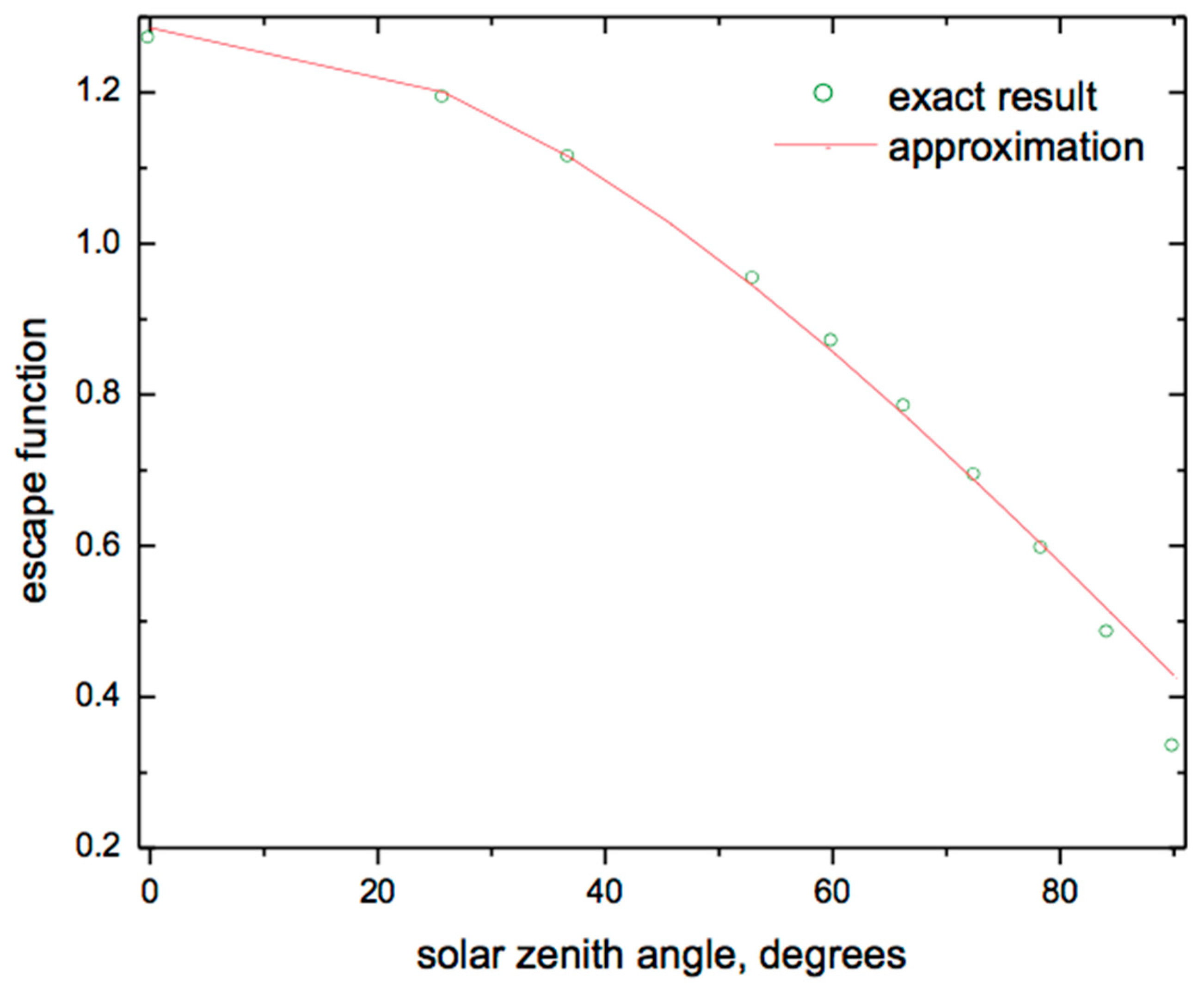
The angular function f satisfies to the reciprocity principle and depends on the viewing/observation geometry via the reflectance of non-absorbing snow layer $R_0$ and via the escape function, which can be approximated by the linear function of the cosine of the viewing zenith angle μ [33]

$$u\left(\mu \right)=\frac{3}{7}\left(1+2\mu \right).$$

(5)

The angular function f also depends on the type of snow/shape of ice crystals (via reflectance/phase function), but not on the snow grain size.

The snow plane albedo $r_p$ can be derived from Equation (1). In particular, it follows by definition that

$$r_p\left({\mu }_0\right)=2 {{\displaystyle \int }}_0^1\overline{R}\left({\mu }_0,\mu \right)\mu d\mu .$$

(6)

where

$$\overline{R}\left({\mu }_0,\mu \right)=\frac{1}{2\pi }{{\displaystyle \int }}_0^{2\pi }R\left({\mu }_0,\mu ,\varphi \right)d\varphi .$$

(7)

where φ is the relative azimuthal angle. The double integral (6) can be evaluated numerically, but we will use the accurate analytical approximation described below. As y → 0, it follows from Equation (1) that

$$R=R_0-u\left({\mu }_0\right)u\left(\mu \right)y.$$

(8)

Because $R_0$ is referred to as a reflecatance for a non-absorbing snow, the double integral (6) with $R=R_0$ is equal to the plane albedo of non-absorbing snow. Therefore, this integral is equal to 1.0 by definition. Then, it follows from Equation (8) (see also Equations (5)–(7)) that

$$r_p\left({\mu }_0\right)=1-y u\left({\mu }_0\right).$$

(9)

We will use the exponential approximation similar to Equation (1)

$$r_p\left({\mu }_0\right)=exp \left(-y u\left({\mu }_0\right)\right).$$

(10)

Equation (10) coincides with Equation (9) as y → 0. However, it can be used in a wider range of the parameter y as compared to Equation (9).

The spherical albedo is defined as

$$r_s=2{{\displaystyle \int }}_0^1{r}_p\left({\mu }_0\right){\mu }_{0}d{\mu }_0.$$

(11)

It follows from Equations (5) and (9) that

$$r_s=1-y.$$

(12)

Therefore, one derives in the framework of the exponential approximation(see Equations (9) and (10))

$$r_s=exp\left(-y\right).$$

(13)

Equation (12) can be used to make an interpretation of the similarity parameter y. Namely, it follows for the absorptance A of the snow layer under the diffuse illumination conditions and small values of the probability of photon absorption

$$A=1-r_s\equiv y.$$

(14)

This means that the parameter y coincides with the value of the snow layer absorptance at small values of the probability of photon absorption in snow. The value of A increases as g (see Equations (3) and (14)) increases as one may expect (stronger forward scattering and, therefore, light penetration to a layer, where light can be effectively absorbed).

It follows from the above equations that the reflectance and plane albedo of snow can be expressed via spherical albedo in the approximation under study

$$R=R_0 r_s^f.$$

(15)

and

$$r_p\left({\mu }_0\right)=r_s^{u\left({\mu }_0\right)}.$$

(16)

It follows from Equations (5) and (16) that the plane and spherical albedo coincide at the cosine of the solar zenith angle equal to 2/3. Equation (15) allows the estimation of spherical (and, therefore, plane albedo (see Equation (16)) from the reflectance measurements at fixed observation geometry avoiding integration procedure as shown in Equations (6), (7), (11). It should be stressed that most of optical instruments do not sample all observation directions; therefore, the theory presented here gives an important hint on how to avoid poor sampling of angular measurements in the procedures for the determination of snow albedo.

2.2. The Accuracy of Exponential Approximation

In this section, we study the accuracy of the presented approximations at various values of the single scattering albedo using the exact radiative transfer calculations. The Henyey-Greenstein phase function

$$p\left(\eta \right)=\frac{1-g^2}{{\left(1+g^2-2g\eta \right)}^{3/2}.}$$

(17)

where η is the cosine of the scattering angle, with the average cosine of scattering angle g = 0.75 similar to that for snow and crystalline clouds, is assumed in all calculations. As a matter of fact, it is not the specific phase function, but rather the average cosine of scattering angle that determines the relationship between R and $R_0$ to be used in this work (see Equation (1)). We assumed an optical thickness of 5000 in our numerical solution of the integro-differential radiative transfer equation for determination of snow reflectance and in the evaluation of the approximations presented in this work. Such an assumption is needed to have the case of a semi-infinite medium considered in the previous section. In this paper, we made use of Intensity and POLarization calculation radiative transfer code (IPOL [34]). IPOL is a Fortran 90/95, BLAS/LAPACK based, discrete-ordinates matrix-operator vector radiative transfer code that computes intensity and polarization (including ellipticity) of the solar radiation reflected from various turbid media. The code also computes planar and spherical albedos by numerical integration of the azimuthally averaged intensity. Recent intercomparison of radiative transfer codes [35] revealed high accuracy of IPOL, including the case of cloud layers, which are in many respects analogous to snowpack.

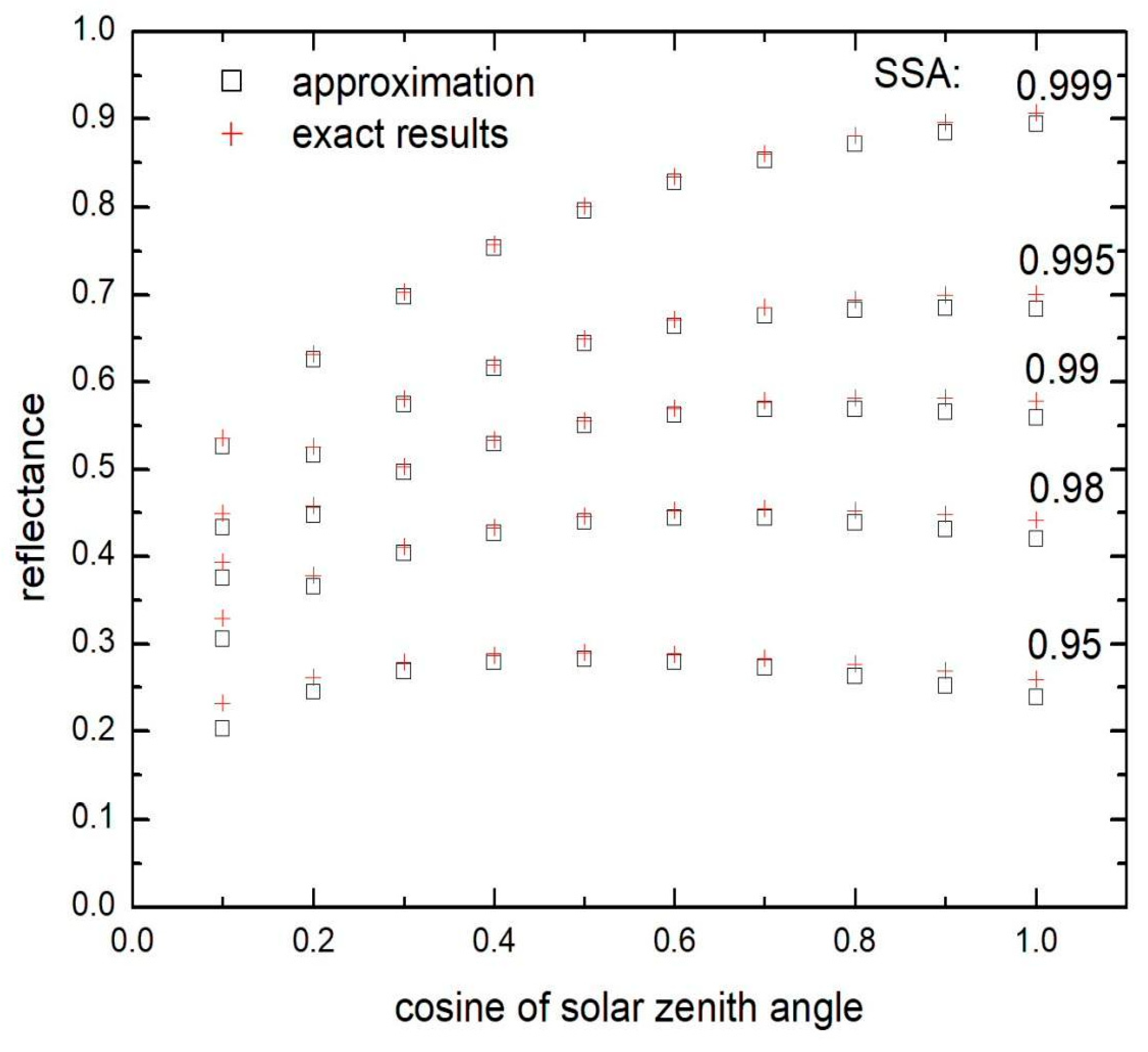
The results of inter-comparison of exact and approximate results for the escape function are illustrated in Figure 1. It follows that the approximation can be used for solar zenith angles under 80 degrees. The accuracy for the reflectance is illustrated in Figure 2 at the nadir observation and for various values of single scattering albedo. It follows that the reflectance decreases for the cases of high solar zenith angles. The reflectance increases for the overhead Sun position. It follows that the approximation is highly accurate even for low (0.2) reflectance values (and PPA equal to 0.05), when the dependence of reflectance on the solar zenith angle is low. 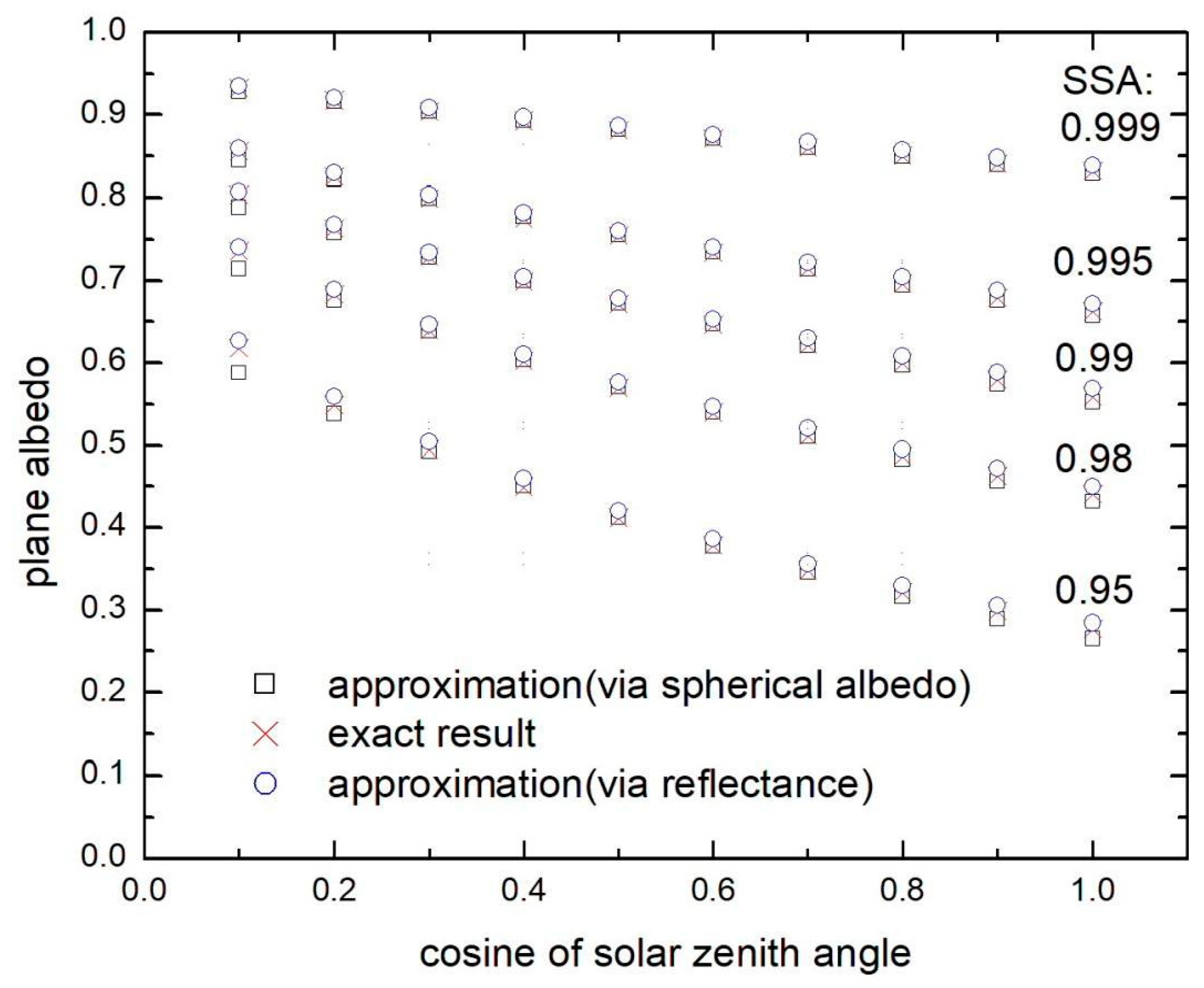The errors are also small (see Figure 3) for the plane albedo in the range 0.3–1.0 typical for clean and polluted snow. 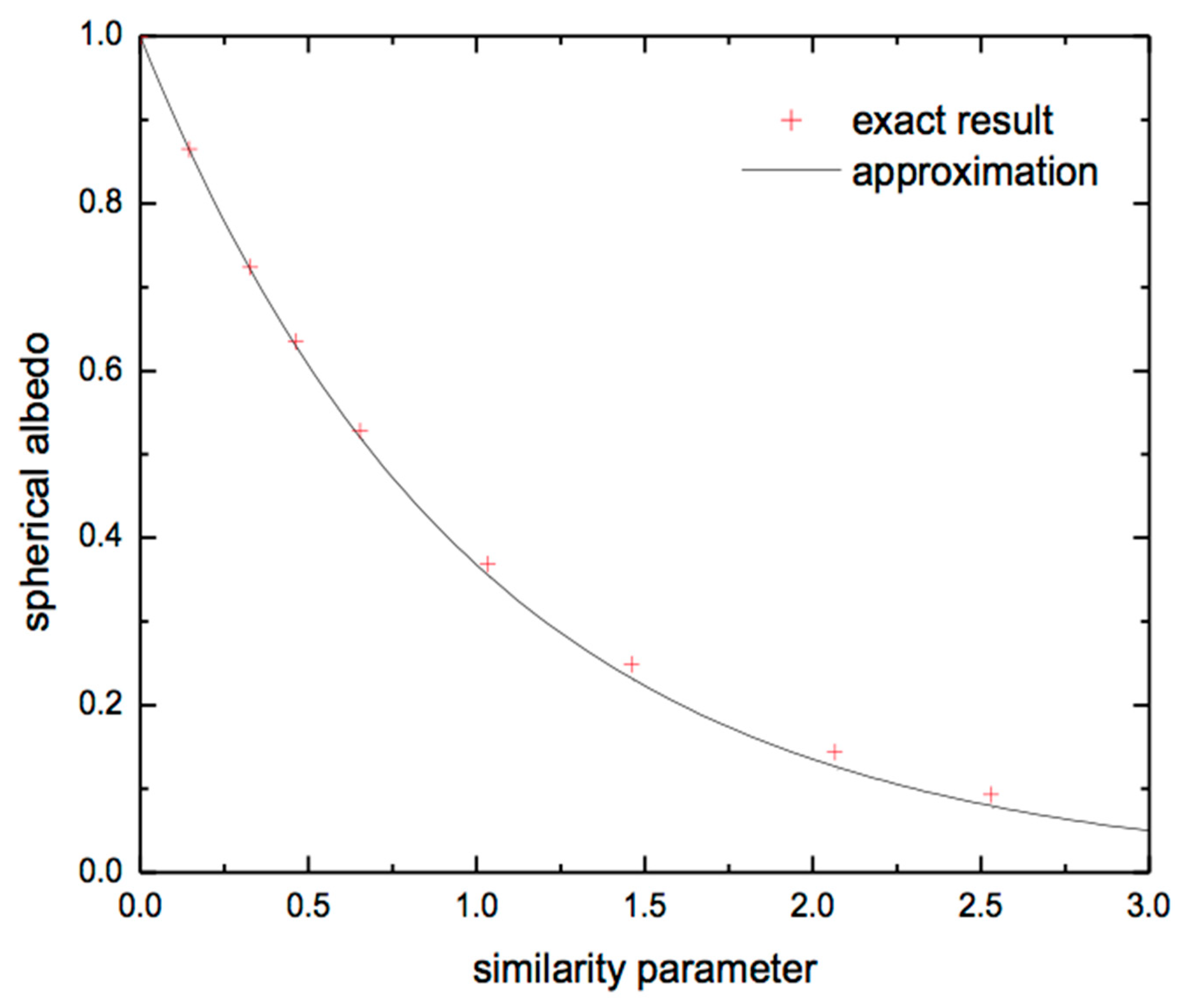In Figure 3, the accuracy of two approximations for the plane albedo is shown (via the similarity parameter y as shown in Equation (10) and also using Equation (16) with spherical albedo derived from Equation (15)). Both approximations produce acceptable results. The accuracy of approximation for the spherical albedo is illustrated in Figure 4. 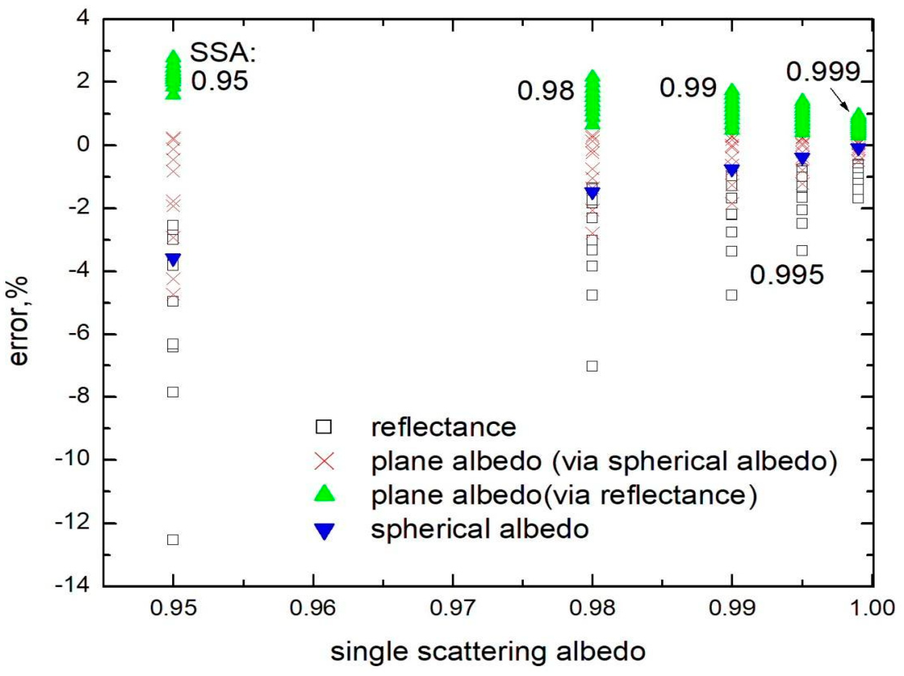It follows that the approximation provides accurate results even at comparatively large values of similarity parameter (y = 2.5). The summary of relative errors for various parameters is illustrated in Figure 5 for the nadir observation case. The spread along the vertical axis is due to solar zenith angle. We conclude that errors are smaller than 5% for the majority of cases. Therefore, the derived approximations are highly accurate and can be used for the solution of the inverse problem: determination of snow properties using optical measurements. Similar conclusions have been reached using a ray tracing model at the grain scale for a wavelength of 1300 nm [36]. A slight discrepancy appeared only at 1550 nm, where the ice absorption is extremely strong [37].

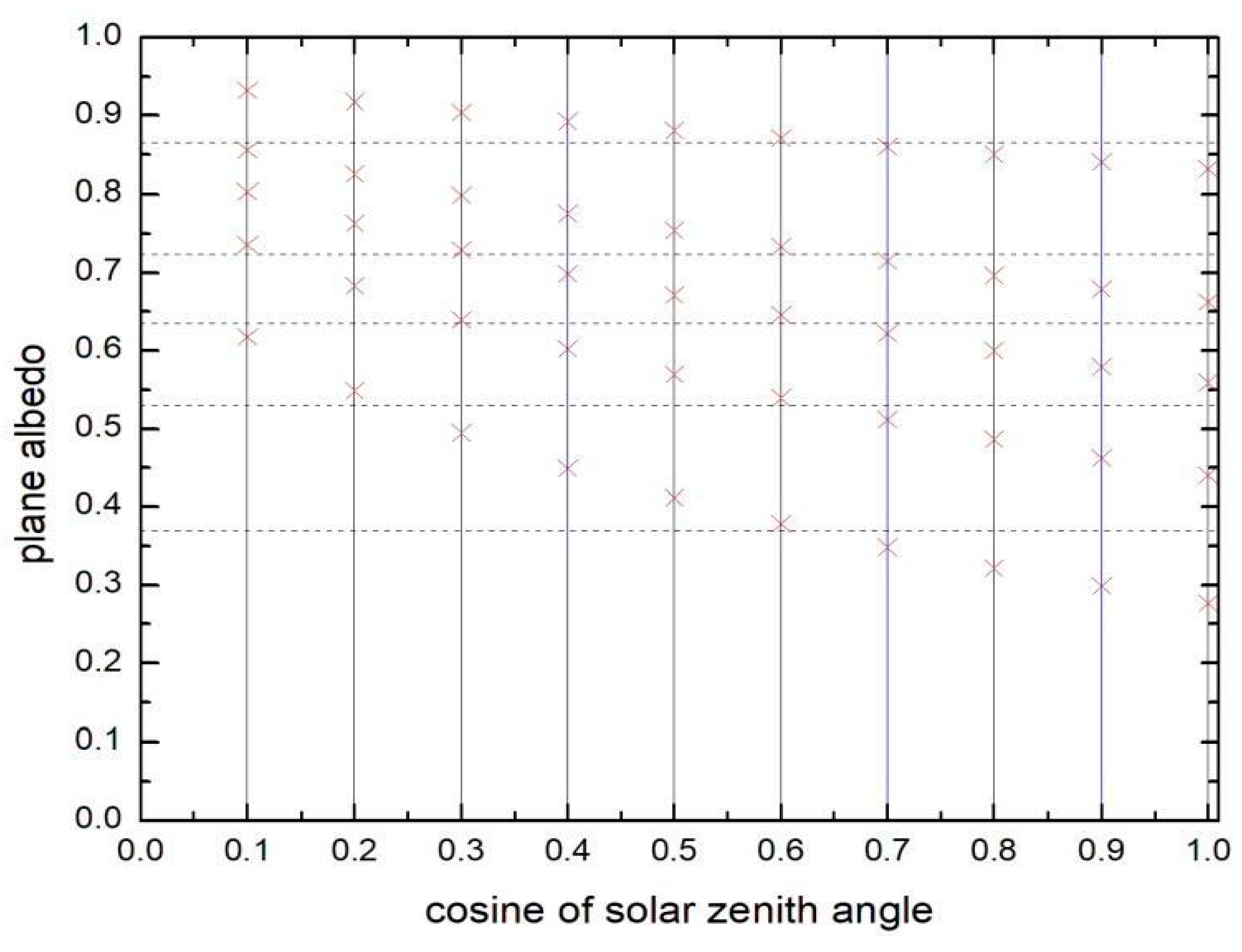
The indirect confirmation of the applicability of the approximate theory also follows from Figure 6, where we present the results of plane and spherical albedo calculations for the various values of single scattering albedo (as in Figure 2). The spherical albedo and planar albedo curves indeed intersect at ${\mu }_0=\frac{2}{3}$, as suggested by the theory presented above. In this case, the solar zenith angle (SZA) is equal to 48 degrees.

3. Results

3.1. The Approximate Solution of the Inverse Problem: Clean Snow

Let us consider first the case of fresh, dry and unpolluted snow. In the 400 nm to 1020 nm spectral range spanned by the OLCI instrument, one can ignore the ice crystal size dependence of the value of the average cosine of scattering angle g.

The parameter β is the ratio of absorption to extinction coefficients

$$\beta =\frac{k_{abs}}{k_{ext}.}$$

(18)

The absorption and extinction coefficients are defined as

$$k_{abs}=N\langle C_{abs}\rangle , k_{ext}=N\langle C_{ext}\rangle .$$

(19)

where $N$ = c/<V> is the number of grains in unit volume of snow, <V> is the average volume of grains and c is the volumetric concentration of grains. Because grains are much larger than the wavelength of the incident light, one may assume [38]

$$\langle C_{ext}\rangle = 2\langle \Sigma \rangle .$$

(20)

where <Σ> is the average cross section of grains (perpendicular to incident light). It is equal to <S>/4 for spherical particles and also convex particles in random orientation [38]. Here, <S> is the average surface area of grains. Assuming that grains are weakly absorbing, which is the case in the visible and near-infrared regions of the electromagnetic spectrum, the following approximation holds [19,39,40]

$$\langle C_{abs}\rangle =B\alpha \langle V\rangle .$$

(21)

where α = 4πχ/λ is the bulk ice absorption coefficient, χ is the imaginary part of ice refractive index and the absorption enhancement factor B depends on the shape of grains but not on the size of grains. The slight dependence of B on the spectral refractive index in the visible and near-infrared can be neglected.

It follows

$$\beta =q\alpha .$$

(22)

where q = B<V>/2<Σ>. Additionally, the following important relationship for the similarity parameter y can be derived using equations given above

$$y=\sqrt{\alpha l}.$$

(23)

where

$$l=\frac{q}{\mathsf{\Lambda }} \mathsf{\Lambda }=\frac{3\left(1-g\right)}{16}.$$

(24)

This equation is highly accurate in the visible and near-infrared wavelengths covered by OLCI. However, it is less accurate at larger wavelengths, where the spectral variation of the asymmetry parameter shall be taken into account. The same is true for Equation (21). The extension of equations to the longer wavelengths in the case of spherical particles has been given in [41] (see also [42]). Taking into account Equation (1), one derives for OLCI channels

$$R=R_{0}exp \left(-f \sqrt{\alpha l}\right).$$

(25)

Therefore, one concludes that the spectral snow reflectance in the visible and near infrared is determined by the spectral bulk ice absorption coefficient and just two additional parameters: the reflectance of a non-absorbing snow and the absorption length $l$. The value of f in Equation (25) is expressed via $R_0$ and the function given by Equation (5). These two parameters can be determined from the measurements at two wavelengths (say, at the OLCI wavelengths 865 nm $({\lambda }_1)$ and 1020 nm $({\lambda }_2)$, see Equation (25)) using [19]

$$R_0=R_1^{\epsilon }{R}_2^{\left(1-\epsilon \right)}.$$

(26)

$$l=\frac{1}{{\alpha }_2{f}^2}ln\left(\frac{R_2}{R_1}\right).$$

(27)

where ${\epsilon }^{}={\left(1-b\right)}^{-1}, b=\sqrt{{\alpha }_1/{\alpha }_2}$ and indices signify the wavelengths used. The error budget for the retrieved parameters $R_{0 }$ and $l$ is presented in Appendix B.

The derived value of $l$ can be used to find the spectral PPA with Equation (22) and the relation (see Equation (24))

$$q=\mathsf{\Lambda }l.$$

(28)

The determination of the parameters given by Equations (26) and (27) makes it possible to find the spectral reflection function, spectral planar and spherical albedos using equations given above (see Equations (13), (16), (23), (25)) in the broad spectral range 300–2400 nm. This is the main idea of this technique. The main point is that the retrieved albedo values are not influenced by the assumption on the shape of particles. The shape effects are accounted for by the value of $l$ found from the measurements.

The snow broadband albedo (BBA) $r_b$ can be determined using the integration of the spectral albedo. In particular, it follows

$$r_b=\frac{{{\displaystyle \int }}_{{\lambda }_s}^{{\lambda }_f}{r}_{p\left(s\right)}\left(\lambda \right)F\left(\lambda \right)}{{{\displaystyle \int }}_{{\lambda }_s}^{{\lambda }_f}F\left(\lambda \right)d\lambda }.$$

(29)

where F(λ) is the incident solar flux at the snow surface, $r_{p\left(s\right)}$ is plane or spherical albedo depending if plane or spherical BBA is of interest. The indices signify the wavelengths used. We have derived the incident solar flux at the snow surface using the Santa Barbara DISORT Atmospheric Radiative Transfer (SBDART) code [43] in the 300 nm to 2400 nm range with the solar zenith angle grid of 1 degree and the following assumptions:

• the water vapor column: 2.085 g/m;
• the ozone column: 0.35 atm-cm;
• the tropospheric ozone: 0.0346 atm-cm;
• the aerosol model: rural;
• the vertical optical depth of boundary layer at 550 nm: 0.1;
• the altitude: 825 m;
• and the surface set to snow, calculated in SBDART using the Mie/δ-Edington model [44] with a snow grain diameter of 0.25 mm.

Generally, the results are only weakly sensitive to the variation of the function F(λ). Therefore, we have used the same solar flux at the snow surface for the retrievals at different geographical locations.

We define the following parameters with Equation (29):

• BBA_visible (300–700 nm),
• near IR BBA_{near IR} (700–2400 nm),
• BBA_shortwave (300–2400 nm).

BBA_visible is the most accurate because the approximations have higher accuracy at small values of the probability of photon absorption. However, the errors of the determination of BBA_{near IR} and BBA_shortwave are small as well because the main contribution to integral (29) comes from the visible and near-infrared regions of the electromagnetic spectrum, where derived equations are very accurate. The values of albedo are retrieved without any assumptions with respect to the particle size or shape. By assuming the snow crystal shape, one may also derive the snow grain size using theory presented above. Namely, let us introduce the effective optical grain diameter

$$d=\frac{3\langle V\rangle }{4\langle \Sigma \rangle }.$$

(30)

Then, the effective diameter can be related to the retrieved value of the absorption length (see Equation (24)) using

$$d=\frac{9l}{16\gamma }.$$

(31)

where γ = B/(1 − g) is the so-called scaling constant. It has been found in [39] from the analysis of experimental data of [45] that the scaling constant is in the range 7.4–11.5 and advised to use the scaling constant value of 9.2. We adopt this value in our study. Then, it follows: d = σ$l$, where σ ≈ 0.06. The values of the pair (B, g) depend on the type of snow/shape of ice crystals [25,46]. In particular, if one assumes that B = 1.6 (as suggested in [40]), one can derive that 1 − g = 0.17 at γ = 9.2, which is smaller as compared to the value of 1 − g = 0.25 used in modern ice cloud remote sensing research [47,48]. This may be due to roundness of grains in snow. Clearly, the retrieved value of d will be biased if the shape of snow grains in the studied snowpack differs from that assumed in the retrieval. Importantly, the dependence on the snow grain shape is influenced by the scaling constant and not by separate values of B and 1 − g. Clearly, more attention must be given to experimental studies of the variability of scaling constant for various types of snow.

We can also retrieve the snow specific surface area. It is related to the diameter d by the following simple equation [36,37,49]

$$s=\frac{6}{\rho d}.$$

(32)

where ρ is the bulk ice density and it has been assumed that the surface area of ice grains is equal to 4<Σ>.

3.2. The Determination of Polluted Snow Properties

3.2.1. Albedo

In the case of polluted snow, we used the above equations, except that the spectral albedo from 400 nm to 1020 nm was derived directly from OLCI measurements. The determination of PPA also needed to be modified. In particular, the following expression for the spherical albedo was used (see Equation (35))

$$r_{s\left(\lambda \right)}={\left[\frac{R_{BOA}\left(\lambda \right)}{R_0}\right]}^{1/f}.$$

(33)

where $R_{BOA}\left(\lambda \right)$ is the bottom of atmosphere snow reflectance. It is derived from the top-of-atmosphere OLCI reflectance accounting for molecular scattering, water vapor and ozone absorption. Aerosol effects are neglected. Equation (33) is applied at the wavelengths 400, 560 and 1020 nm. The value $R_0$ is derived using equations presented in Appendix C. The planar albedo is found from Equations (16) and (33).

For the BBA calculation, we needed values of spectral albedo in the 300 nm to 2400 nm range. We approximated the derived spherical albedo spectra (see Equation (33)) in the range 300 nm to 1020 nm for polluted snow by the quadratic polynomial using the measurements at 400 nm, 560 nm and 1020 nm least influenced by gaseous absorption (except ozone at 560 nm). The derived polynomial was then used for the determination of PPA for the case of polluted snow (see Equations (3) and (13))

$$\beta \left(\lambda \right)=\mathsf{\Lambda }l{n}^2\left(r_{s\left(\lambda \right)}\right).$$

(34)

The albedo values at the wavelengths longer than 1020 nm needed for the evaluation of BBA were found using Equations (10) and (13) as for clean snow. This is possible because the influence of pollutants on snow reflectance spectra is less pronounced or negligible in the near-infrared, where ice grains themselves are strong absorbers of radiation.

In the case of clean snow, only the wavelengths 865 nm and 1020 nm were used in our retrieval. Therefore, the errors due to uncertainties of atmospheric correction [50] were minimized. In the case of polluted snow, albedo was derived using the measured OLCI top-of-atmosphere reflectance also at channels 400 and 560 nm, which were influenced by the optical properties of atmosphere to a much greater extent (e.g., molecular and atmospheric aerosol scattering/absorption), see also [20]. It is expected that the derived parameters for the polluted snow have larger errors as compared to those for unpolluted snow due to the problems of atmospheric correction over snow-covered areas.

3.2.2. Snow Grain Size and Absorption Coefficient of Pollutants

The snow grain size and absorption coefficient of pollutants in the case of polluted snow is found as explained below. It is assumed that the reflection function of polluted snow is described by Equation (15)

$$R=R_0{r}_s^f.$$

(35)

with (see Equation (13))

$$r_s=exp\left(-y\right).$$

(36)

where

$$y=4\sqrt{\frac{\beta }{3\left(1-g\right)}}.$$

(37)

$$\beta =\frac{k_{abs}}{k_{ext}}.$$

(38)

We shall assume that the scattering and extinction of light by pollutants is much smaller than that of ice grains and absorption coefficient of pollutants can be approximated as

$$k_{abs, pol}\left(\lambda \right)=k_{abs, pol}\left(\lambda ={\lambda }_0\right){\left(\frac{\lambda }{{\lambda }_0}\right)}^{-m}.$$

(39)

where ${\lambda }_0$ = 1 μm. Then, it follows for the polluted snow reflection function

$$R=R_{0}exp \left(-4f\sqrt{\frac{\left(B\alpha c+\kappa {\tilde{\lambda }}^{-m}\right)d}{3\left(1-g\right)c}}\right).$$

(40)

where $\kappa \equiv k_{abs, pol}\left({\lambda }_0\right), \tilde{\lambda }=\frac{\lambda }{{\lambda }_0}$. We have used the geometrical optics result for the snow extinction coefficient $k_{ext}=\frac{3c}{d}$ (see Equations (19), (20) and (30)) $\mathrm{and} \mathrm{the}$ following relationship for the absorption coefficient of polluted snow in the framework of the impurity external mixture approximation

$$k_{abs}=k_{abs, ice}+k_{abs, pol}.$$

(41)

where (see Equations (19), (21) and (30))

$$k_{abs, ice}=B\alpha c.$$

(42)

Using the absorption length $l$ (see Equation (24)), one can derive from Equation (40)

$$R=R_{0}exp \left(-f\sqrt{\left(\alpha +\tilde{k}{\tilde{\lambda }}^{-m}\right)l}\right) .$$

(43)

where $\tilde{k}=\frac{k}{B c}$.

Equation (43) can be used to solve the inverse snow remote sensing problem using spectral reflectance measurements. There are four unknown parameters to be found using Equation (43): $l, m, R_0, \widetilde{k.}$ They can be found numerically (e.g., using optimal estimation approach) or analytically under the assumption that pollutants do not influence reflectance in the near infrared (say, at 865 and 1020 nm for OLCI). We used the second approach. Then, one can derive [20]

$$R_0=R_3^{\epsilon }{R}_4^{\left(1-\epsilon \right)}, l=\frac{1}{{\alpha }_4{f}^2}l{n}^2\left(\frac{R_4}{R_0}\right), m=\frac{ln \left(\frac{p_1}{p_2}\right) }{\ln \left(\frac{{\lambda }_2}{{\lambda }_1}\right)}, \tilde{\kappa }=\frac{p_1{\tilde{\lambda }}_1^m}{f^{2}l}.$$

(44)

where

$$\epsilon =\frac{1}{1-b}, b=\sqrt{\frac{{\alpha }_3}{{\alpha }_4}}, p_k=l{n}^2\left(\frac{R_k}{R_0}\right).$$

(45)

Symbols 1–4 signify the wavelengths used (400, 560, 865 and 1020 nm, respectively, for OLCI). These equations are used to derive the snow grain diameter (see Equation (31)) and also the absorption coefficients of pollutants (see Equation (39)) normalized to the concentration of snow grains (snow density). The error budget for the determination of parameters given by Equations (44) is discussed in Appendix D.

3.3. Snow Properties Processor for SNAP

The Snow Properties Processor (SPP) has been developed and implemented under the framework of the European Space Agency (ESA) Sentinel-3 for Science (S34Sci) Land Study 1: Snow that delivered a SNAP plug-in. The processor version 2.3 provided the implementation of the algorithms as described above for the various snow properties. As input, the processor requires an OLCI L1b product that is atmospherically corrected and cloud screened in pre-processing. The output was a set of snow properties, defined by the user via processing parameters. Atmospheric correction was performed ignoring effects of aerosol scattering and absorption. Molecular scattering and absorption was fully accounted for as provided by the SNAP by default.

When the Snow Properties Processor was called from its menu entry in the SNAP desktop application, the processor Graphic User Interface was displayed. It contains two tabs ‘I/O Parameters’ and ‘Processing Parameters’ (Figure 7). Here, I/O stands for Input/Output.

The most important processing parameters, which can be set by the user, are as follows:

• Select OLCI wavelengths for spectral snow quantities: for the selected wavelengths, the computed spectral snow quantities (i.e., spectral snow albedo) were written as the corresponding band into the target product.
• Name of binary mask band in cloud classification product (if present): see details in the software user manual at https://readthedocs.org/projects/s3tbx-snow/.
• Consider snow mask based on the OLCI Normalized-Difference Snow Index (NDSI): if selected, an NDSI value will be computed from atmospherically corrected reflectances at wavelengths 865 nm and 1020 nm (NDSI = (R(865 nm) − R(1020 nm))/(R(865 nm) + R(1020 nm)). If this value exceeded 0.03 (and reflectance at 410 nm > 0.5), the given pixel was regarded as a snow pixel. The normalized bare ice index (NDBI) was also provided in the output. It was defined as NDBI = (R(410 nm) − R(1020 nm))/(R(410 nm) + R(1020 nm)). It was assumed that the values of NDBI below 1/3 corresponded to snow and the ice was assumed for values of NDBI above 1/3. The dark bare areas correspond to values of NDBI above 2/3. OLCI snow mask is given in output (snow mask was equal to 1 for 100% snow pixels. Otherwise, the snow mask was zero).
• Consider snow pollution: if selected, a retrieval for polluted snow was applied for the considered snow pixel.
• Compute PPA: if selected, the spectral probability of photon absorption (PPA) was written to the target product for each selected OLCI wavelength.
• OLCI reference wavelength: reference wavelength used in the snow property algorithms.
• OLCI gain for band n: OLCI system vicarious calibration (SVC) gain for the relevant bands (n = 1, 6, 17, 21 (400, 560, 865, 1020 nm)) used in the retrieval algorithms outlined above.

More details on this can be obtained from the SNAP processor help documentation and from the software user manual (see above). The result product from the snow properties processor contains various snow properties, depending on the processing parameters specified by the user. The bands which can be generated are presented in

Table 1. Bands in the final snow properties product.

Name in Product	Units, When Not Dimensionless	Description
albedo_bb_spherical_vis		Spherical albedo in the broadband visible range from 300 nm to 700 nm
albedo_bb_spherical_nir		Spherical albedo in the broadband near infrared range from 700 nm to 2400 nm
albedo_bb_spherical_sw		Spherical albedo in the broadband shortwave range from 300 nm to 2400 nm
albedo_bb_planar_vis		Planar albedo in the broadband visible range from 300 nm to 700 nm
albedo_bb_planar_nir		Planar albedo in the broadband near infrared range from 700 nm to 2400 nm
albedo_bb_planar_sw		Planar albedo in the broadband shortwave range from 300 nm to 2400 nm
albedo_spectral_spherical		Spectral spherical albedo in 21 OLCI bands
albedo_spectral_planar		Spectral planar albedo in 21 OLCI bands
rBRR		Estimated bottom of atmosphere OLCI reflectance in 21 OLCI bands
ppa_spectral		PPA in 21 OLCI bands
grain_diameter	mm	Snow grain diameter
snow_specific_area	m2 kg−1	Snow specific surface area
ndbi		Bare ice indicator
pollution_mask		Pollution mask
$\tilde{k}$	mm−1	Normalized snow impurity absorption coefficient at 1 µm
l	mm	Effective absorption length
m		Absorption Angstrom parameter
r_0		Reflectance of non-absorbing snow layer
f_rel_err		Relative error of normalized snow impurity absorption coefficient at 1 µm
l_rel_err		Relative error of parameter l
m_rel_err		Relative error of parameter m
r_0_rel_err		Relative error of parameter r_0
ndsi		Normalised differential snow index
ndsi_mask		NDSI mask for snow identification
quality_flags		L1b quality flags
pixel_classif_flags		Pixel classification flags

.

3.4. Cloud Identification

Cloud screening of Antarctic and Col du Lautaret (French Alps) OLCI scenes used for the SPP validation studies is achieved by rejecting mostly cloudy scenes identified by visual inspection. The cloud cover in the vicinity of the field location (approximately 10 × 10 pixels) was visually assessed using RGB true-color composites generated from OLCI bands 4, 6 and 8, and classified in three categories: cloud-free, partly-cloudy and fully-cloudy. Owing to the availability of the scenes (multiple daily acquisitions), only the cloud-free images were retained for this study.

For Greenland, we have found that the majority of clouds pixels can be identified in OLCI imagery using a simple thresholding of snow grain diameter for values less than 0.1 mm or OLCI band 21 (1020 nm) bottom of atmosphere reflectance exceeding 0.72. Residual cloud effects include cloud shadows and thin clouds.

Cloud conditions are constrained for Greenland validation studies with PROgramme for Monitoring Greenland ICE Sheet (PROMICE) ground observations using a cloud probability index (CPI) estimated from PROMICE automatic weather station longwave downward irradiance (L↓) after [51]. CPI is approximated from the bi-modality of L↓, i.e., clear or cloudy, and its partial impact on near surface temperature T. The dependence of L↓ on T is evaluated at each PROMICE site [52] and showed agreement with the blackbody theory, i.e., L↓ = εσTQ. For overcast conditions, ε was found to be 0.993 and Q was 4, approaching near blackbody radiative dependency. The parameter σ is the Stefan-Boltzmann constant (5.67 × 10⁻⁸ ${\mathrm{Wm}}^{-2}{\mathrm{K}}^{-4}$). For clear conditions the best fit to the fifth percentile resulted in variable values of ε and Q. Linear interpolation between the clear and cloudy estimates produces CPI values from zero to one for pairs of hourly L↓ and T measurements. Values below and exceeding the range of theoretical L↓ values were assumed to have been recorded respectively in clear and overcast conditions, i.e., CPI = 0.0 and CPI = 1.0.

Polar aerosols have typically low optical thickness (below 0.1 at the at 550 nm), have little influence on the top-of-atmosphere reflectance at the near-infrared wavelengths beyond ~865 nm [53], and thus, were currently neglected.

3.5. Validation of Snow OLCI Products

3.5.1. Snow Spectral Albedo

The spectral planar albedo products derived from OLCI scenes were compared to ground measurements of surface albedo. In a first step, the accuracy of the OLCI albedo product and its ability to capture the temporal evolution of the surface, and thus seasonal trends, was assessed using a dataset of sub-hourly observations of spectral surface albedo obtained at a fixed location at Dome C, Antarctica (75°06′00″S, 123°19′58″E, 3233 m elevation). Instrumentation details are provided below. In a second step, the evaluation of the OLCI spectral planar albedo retrievals at multiple locations spreading across the Antarctic plateau with varying snow surface properties was performed using portable spectral albedo measurements obtained along a 1371 km transect south of Dumont d’Urville (66°39′47″S, 140°00′10″E, 202 m). In a third step, the OLCI spectral planar albedo retrievals of snow containing impurities (atmospheric mineral aerosol deposits) were compared to portable spectral albedo measurements performed at Col du Lautaret, in the French Alps (45°02′07″N, 6°24′20″E, 2000 m), after a Saharan dust deposition event.

Data Processing and Instrumentation

An OLCI database was created for the different validation sites, applying the following steps. For each of the validation datasets, the OLCI L1c full-resolution products overlapping the location of the field measurements for the dates corresponding to the ground-based acquisitions were gathered. The Snow Properties Processor was run for all the remaining OLCI scenes, and the values for the pixels overlapping the field sites were extracted from the product. For all OLCI scenes, the SPP was run for the 21 OLCI bands, using band 21 (1020 nm) as the reference wavelength. In this study, the OLCI SVC gains (described in Section 3.3, see Figure 7) were not applied. For the scenes in Antarctica, the SPP was run without applying the snow pollution algorithm, whereas for the Col du Lautaret scenes, the snow pollution algorithm was used.

Spectral albedo measurements of the snow surface were acquired at Dome C using the Autosolexs instrument [22,54,55], an automated spectral-radiometer that has been acquiring surface albedo measurement every 12 min between October and March since 2012. The instrument, shown in Figure 8, is described in detail in [22], and therefore only a succinct description is provided here.

Autosolexs is composed of two measurement heads located approximately 1.5 m above the surface, each containing two upward and downward facing cosine receptors. The downward facing collectors were estimated to receive 75% of the reflected signal from the surface from an area of approximately 3.5 m in radius [22]. The receptors are connected to an Ocean Optics Maya2000 Pro spectrometer with fiber optics passing through an optical switch. Autosolexs measures the downward and upward (reflected) solar radiation. Using the calibration and processing steps described in [22], the spectral albedo was calculated as the ratio of the upwelling to downwelling spectral irradiances, providing usable data across the 400–1050 nm range. Owing to the negligible amount of diffuse illumination, the bi-hemispherical reflectance measured by the instrument (here called albedo) was directly compared to the directional–hemispherical reflectance (planar albedo) retrieved from OLCI images. For the validation purposes of this study, the datasets of the 2016–2017 and 2017–2018 summer seasons were used. The comparison between the ground observations and the satellite retrievals of spectral albedo was performed in several steps. Over the two summers, 1151 OLCI scenes were available at the Dome C location. For each scene, the closest Autosolexs albedo measurement in time was selected. To avoid a bias due to the albedo changing with the SZA and possibly changing snow physical properties, Sentinel-3 scenes more than 15 min apart from an Autosolexs measurement were automatically discarded. A second filter was applied to remove the measurements performed with a SZA larger than 75°, as it was shown in [22] that large SZA values introduce significant variations in the Autosolexs measurements. The remaining measured albedo spectra were smoothed with a 5 pixe-wide averaging sliding window to remove excessive noise due to instrument oversampling. For each measurement the spectra from the two heads of the instrument were averaged, allowing to diminish the effect of small-scale local surface roughness features [56], that may be located beneath the instrument, introducing a bias in the measurements owing to the small footprint of the instrument (approximately 40 ${\mathrm{m}}^2$). After the processing steps described above, 252 OLCI scenes were retained for comparison with the Autosolexs instrument over the two seasons. Although the full measured spectra are shown in Figure 9, in order to compare the ground values with each individual Sentinel 3 OLCI band the measured albedo was spectrally integrated over each bandwidth using the average spectral response provided by ESA.

For the spatial validation of the satellite albedo retrievals, the OLCI planar spectral albedo was compared to measurements obtained along a 1371 km transect on the Antarctic plateau south of the French Dumont d’Urville research station, over a period of 34 days between December 2016 and January 2017. The measurements were obtained within the framework of the ASUMA program (Improving the Accuracy of the SUrface Mass balance of Antarctica). Albedo measurements were taken at 23 locations along the transect (

Table 2. Location, Sentinel-3 acquisition dates and times, and SZA values for the sites along the ASUMA traverse used for the validation of the spectral albedo products.

Site Name	Sentinel-3 OLCI Acquisition Date/Time (UTC)	SZA/°		Average Latitude/Longitude of the Field Measurements
		S3 Overpass	Measurement
st1	2016/12/01, 22h21	59.14	64.1	−66.881150, 139.280006
st2	2016/12/02, 23h36	52.81	47.2	−67.167791, 138.968926
st6	2016/12/06, 21h51	63.25	68.5	−68.872819, 135.303749
st10	2016/12/10, 23h28	55.23	67.6	−69.636122, 135.279596
st16	2016/12/16, 22h32	58.60	70.8	−69.953844, 138.551435
st17	2016/12/17, 22h06	60.74	70.8	−69.953799, 138.553538
st21	2016/12/21, 22h02	60.01	75.6	−69.786595, 141.972969
st22	2016/12/22, 23h17	54.20	64.9	−69.786595, 141.972969
st25	2016/12/25, 23h40	53.39	64.7	−69.376932, 139.016187
st26	2016/12/26, 23h13	55.53	67.4	−69.060033, 138.225079
st27	2016/12/27, 22h47	57.90	55.3	−68.747273, 137.443734

) using the Solalb instrument (shown in Figure 8, a handheld version of Autosolexs). The instrument is composed of a 3 m boom at the end of which a light-collector is connected. It is characterized by a cosine response. The light-collector is connected to the same spectrometer model used in Autosolexs (Maya200pro, Ocean Optics) via an optic fiber. The instrument measures incoming radiation over the wavelength range 200–1300 nm with a usable range of 400–1050 nm. To measure albedo, the light-collector was first placed horizontally, in an upward-looking position to collect the incident irradiance, then in a downward-facing position to collect the upwelling reflected solar radiation from the snow surface. Following the processing chain developed for Autosolexs [22], the albedo was calculated as the ratio of reflected to incident solar radiation. For each of the 23 locations, multiple albedo measurements were performed at random positions within a radius of approximately 100 m, and the coordinates were recorded with a handheld GPS. The series of individual measurements at each location were averaged and compared to the corresponding OLCI retrieval for the overlapping pixel. The variance of the measurements was considered to represent the sub-pixel spatial variability of the pixel. For each set of field measurements, the closest cloud-free OLCI overpass in time was selected. If no OLCI cloud-free scenes were available on the day of the field measurements, the dataset was discarded. Because of the difference in time between the satellite overpass and the ground measurements, and thus the difference in SZA (Table 2), the measured albedo was converted to planar spectral albedo and corrected for the difference in SZA based on the asymptotic analytical radiative transfer theory presented in [19]. A full description of the processing is available in Appendix E. After these processing steps, 11 OLCI scenes were retained for comparison with the Solalb measurements.

The OLCI albedo retrievals for polluted snow were validated using portable spectral albedo measurements obtained with the Solalb instrument previously described, at the Col du Lautaret field site with neighboring slopes of ~4°. Measurements were made on the 17, 19 and 24 April 2014 after Saharan mineral dust deposition events 14–16 and 22–23 April 2018. To minimize the effects of topography, the ground measurements acquired on 17 April were collected over a relatively flat (average slope of 3.2°) area of the plateau. Five spectral albedo measurements were obtained at random within a radius of approximately 10 m, with an average SZA of 55.3°. The averaged measurements were compared to the overlapping OLCI pixel (SZA = 41.2°). On 19 April, six surface albedo measurements were obtained every 40 m along a 240 m transect, to account for the spatial variability of the snow surface (slopes, snow physical properties, deposited dust). The average slope along the transect was 8.6° and the average SZA at the time of the field acquisitions was 40.9°. The entire transect was contained within an OLCI pixel, allowing a comparison of all the measured points with the satellite retrieval (SZA = 39.2°) obtained on the 20 April owing to the lack of Sentinel 3 data on 19 April. The comparison was considered valid, owing to the stable weather conditions during the two days. On 24 April, measurements were obtained at 24 locations along a 420 m transect on the plateau covering three OLCI pixels. However, two of the pixels contained only three and four measurements, respectively, located along the edge of the pixels, and thus, they were discarded, since the measurements were not considered representative of the pixels. Therefore, 17 measurements were retained for the comparison with the overlapping OLCI pixel. The slopes measured along the transect on the 24 April (average slope: 10.6°) were more pronounced than the slopes measured on the other dates. The SZA at the time of the field measurements was similar to the SZA at the time of the OLCI overpass with values of 36.5° and 36.9°, respectively.

Once processed, the albedo spectra were corrected for the difference in configuration between the measurement setup and the satellite retrievals. The ground spectral albedo acquisition was performed over sloping terrain, with a horizontal sensor, whereas the theory used in the retrievals assumes a horizontal surface. It is known that the surface albedo measurements are affected by the departure of the surface from horizontal [54], and therefore, the ground measurements need to be corrected for a direct comparison with the satellite spectral albedo. A full description of the algorithm appears in Appendix E. Furthermore, the difference in SZA between the ground acquisitions and the satellite overpass was accounted for, as described for the processing of the ASUMA dataset. Finally, for each date the albedo measurements were averaged, and compared to the closest spectral planar albedo retrieval in time for the overlapping OLCI pixel.

Clean Snow

The spectral performance of the snow albedo retrieval algorithm is illustrated in Figure 9, where the OLCI snow spectral planar albedo retrievals at all 21 bands are compared to the concurrent. Autosolexs spectral albedo measurements for four dates selected across the 2016/17 and 2017/18 seasons. We have applied a scaling factor to the Autosolexs data to compensate measurement artifacts [22,54]. The scaling factor is obtained by fitting a two-parameter model to the observed spectrum in the 700–1050 nm range [22]. This leads to the ground measured plane albedo variability, which may be induced by surface roughness.

An excellent agreement across the wavelength range was observed, particularly for the two retrievals at smaller SZAs (<70°), where the satellite albedo values were within 2% of the ground measurements for all OLCI bands. For the retrievals with a SZA close to 70°, despite an overall good agreement, slightly more variability between observed and retrieved albedo was detected at larger wavelengths. This can be related to surface roughness effects, or problems with the atmospheric correction in case of large values of SZA.

The four dates illustrated in Figure 9 were selected to show the high radiometric accuracy of the retrievals, and are mostly representative of the two summer seasons at Dome C. It follows from

Table 3. Comparison between the Sentinel-3 OLCI spectral planar albedo retrievals and the Autosolexs spectral albedo measurements over the 2016–2017 and 2017–2018 summers at Dome C, Antarctica. The standard deviation is calculated from the measurements or OLCI retrievals performed over the 2 years, representing the variability of the snow conditions. The mean albedo bias column shows that the error of retrievals is below 1% for all channels below 1020 nm and approximately 2% at 1020 nm.

Sentinel-3 OLCI Band	Sentinel-3 OLCI Spectral Planar Albedo Retrievals		Autosolexs Spectral Albedo Measurements		Mean Albedo Bias (Absolute):	Mean Albedo Bias (%):
	Average	Std	Average	Std
01 (400 nm)	0.9988	0.0002	0.9899	0.0210	0.0089	0.9446
02 (421.5 nm)	0.9987	0.0002	0.9941	0.018	0.0046	0.4991
03 (442.5 nm)	0.9981	0.0003	0.9962	0.0136	0.0019	0.2099
04 (490 nm)	0.9955	0.0006	0.9971	0.0086	0.0016	0.1572
05 (510 nm)	0.9938	0.0008	0.9965	0.0061	0.0027	0.2651
06 (560 nm)	0.9889	0.0015	0.9929	0.0044	0.0039	0.3951
07 (620 nm)	0.9819	0.0024	0.9893	0.0040	0.0075	0.7550
08 (665 nm)	0.9749	0.0034	0.9812	0.0052	0.0062	0.6345
09 (673.75 nm)	0.9742	0.0034	0.9793	0.0052	0.0050	0.5133
10 (681.25 nm)	0.9731	0.0037	0.9776	0.0052	0.0045	0.4581
11 (708.75 nm)	0.9663	0.0046	0.9706	0.0057	0.0043	0.4466
12 (753.75 nm)	0.9575	0.0057	0.9574	0.0063	0.0001	0.0112
13 (761.25 nm)	0.9536	0.0062	0.9584	0.0072	0.0047	0.4905
14 (764.375 nm)	0.9524	0.0064	0.9544	0.0072	0.0020	0.2072
15 (767.5 nm)	0.9508	0.0066	0.9510	0.0073	0.0003	0.0270
16 (778.75 nm)	0.9452	0.0073	0.9455	0.0078	0.0002	0.0248
17 (865 nm)	0.9213	0.0104	0.9226	0.0099	0.0013	0.1444
18 (885 nm)	0.9055	0.0124	0.9056	0.0118	0.0001	0.0050
19 (900 nm)	0.8992	0.0132	0.8975	0.0127	0.0017	0.1906
20 (940 nm)	0.8875	0.0146	0.8908	0.0147	0.0032	0.3576
21 (1020 nm)	0.7939	0.0254	0.8075	0.0258	0.0136	1.6661

that the mean albedo bias over the two years was less than 1% for all bands below 1020 nm and it was smaller than 2% at 1020 nm. Considering the individual comparisons between the OLCI retrievals and the Autosolexs measurements at two wavelengths (865 and 1020 nm) in Figure 10, the values were well distributed along the identity line at 865 nm, and the satellite retrievals were mostly within 2% of the ground measurements for all dates, highlighting the ability of the retrieval algorithm to capture temporal variations. At 1020 nm, although the average bias is low, the retrievals tended to underestimate albedo in comparison to the ground measurements. Dependency of the satellite retrievals to the SZA is evident, with 90% of the points underestimating the albedo by more than 2% having SZA over 65°.

The validation of the OLCI spectral albedo retrievals for varied snow surface conditions across the Antarctic plateau is illustrated in Figure 11, where the average albedo measured with the Solalb instrument at each site and its standard deviation, representing that the subpixel variability is shown for four wavelength bands. Although the inter-site variability is low across the 1371 km transect, the wide error bars provide an indication of the strong sub-pixel spatial heterogeneity at each of the individual sites. Since the retrieved satellite albedo and the field measurements are not directly comparable owing to the differences (2.6 to 15.6°) of the SZA between the satellite overpasses and the measurements (Table 2), the measured albedo corrected for the SZA at the time of the overpass is also illustrated in Figure 11, with the assumption that the snow surface conditions did not change during the day. The data suggest an excellent radiometric accuracy between the spectral albedo and the retrieved satellite spectral albedo across the sites. Differences between the albedo estimated from the ground measurements and the satellite retrievals occur at 1020 nm, which we suspect is the result of the heterogeneity of the physical properties of the snow surface and could be explained by the under-representation of the pixel by the measured points (not shown here).

The comparison of OLCI spectral planar albedo with spectral surface albedo measurements at the Dome C site over 2 summer seasons shows that the OLCI snow products can be used to accurately monitor the albedo of clean snow surfaces and their temporal evolution over flat surfaces (see Table 3). However, the data have also shown that biases are introduced in the albedo retrieval algorithm for large SZAs. A part of uncertainty in the validation results remains due to differences introduced by the point-to-pixel comparison which does not account for the spatial heterogeneity (albeit low in the case of Dome C) and other scale effects.

Polluted Snow

The OLCI retrievals of spectral planar albedo using the snow pollution branch of the retrieval algorithm for three dates at the Col du Lautaret validation site (see Figure 12) are illustrated in Figure 13. The OLCI retrievals were compared to ground measurements from a single location on 17 April 2018 and along transects on the 19 and 24 April 2018. The calculated planar albedo accounting for the slope under the sensor and the SZA at the overpass time, and the spatial variability of the measurements are also illustrated in the figure. For the three dates, the figure highlights the ability of the algorithm to retrieve the spectral signature of the snow containing dust, i.e., with enhanced absorption in the 400 nm to 650 nm range [25]. The measurements obtained at a single location on 17 April 2018 and along a transect across a homogenous slope on 19 April 2018 exhibited little sub-pixel variability, indicating similar snow physical properties and dust concentrations across the site (see Figure 12). On the other hand, the transect performed on 24 April 2018 across a larger range of slopes, suggests a greater variability of the snow surface, probably owing to the differences in snow properties between the north and south facing slopes. When taking into account the slope and difference in SZA between the measurement and the satellite retrieval, an excellent agreement was observed on 17 April 2018. On 19 April 2018, a good agreement was also observed, with an overestimation of the OLCI retrieval between 400 and 510 nm and between 940 and 1020 nm. Nevertheless, the satellite retrieval is able to estimate the overall spectral shape of the polluted snow surface. On 24 April, the OLCI retrieval overestimated the albedo at all wavelengths, with differences between ground and OLCI albedo of 8% at 400 nm and 16% at 1020 nm. The disagreement between the OLCI retrieval and the measurements on the last date may be explained by the larger slopes across the pixel (10.6°), the higher sub-pixel variability in the measurements, and the location of transect on the plateau, closer to surrounding topographic features than the sites measured on the two previous days. Indeed, the measurements made on 17 and 19 April 2018 were obtained in flatter terrain (average slopes of 3.2° and 8.6°, respectively) and further away from large surrounding topographic features (cliffs, peaks), which have been shown to significantly impact satellite measurements due to the interactions between the solar radiation and the topographic features [54]. Therefore, in the configuration of 24 April 2018 the effect of the slope can not be accounted for using the algorithm described in Appendix E.

3.5.2. Broadband Albedo

Data Processing and Instrumentation

In Greenland, snow and ice albedo was monitored by the Programme for Monitoring of the Greenland Ice Sheet automatic weather stations (AWSs) located at 24 sites on the Greenland ice sheet (Figure 14). The PROMICE AWS record shortwave irradiance upward and downward (300 nm to 2400 nm) each 10 min using a Kipp CM3 pyranometer as part of a Kipp CNR-1 or CNR-4 radiometer bundle (see Figure 13). The CM3 thermopile is covered by a single glass dome and complies with ISO 9060 s-class specifications, i.e., ±10% accuracy for daily totals. Under conditions with no frost or water on domes and a level station, as is common here, the CM3 performs better than ±5%. PROMICE AWS tilt measurements (see Figure 14) were used to exclude cases having tilt greater than ±1.5 degrees. Furthermore, to avoid larger measurement uncertainty, albedo values include only those instantaneous measurements for which sunlight incidence angle for both the ice sheet surface and the upper dome of the sensor was larger than 20 degrees.

In an effort to neutralize PROMICE station shortwave radiation obstruction effects by the AWS measurement platform, we apply the correction used in [56] (equation 16). An assumption was that the OLCI BBA_shortwave for dry clean snow had no bias, as shown for clean snow in the Antarctica spectral albedo validation. In the correction, we assumed a constant station (mast, enclosure, solar panel) average reflectivity of 0.4, and a fraction of station obstruction coming from above and below the pyranometer. We used a variable [56] measurement frame obstruction “f” parameter to produce zero average bias with the OLCI retrieval for dry snow, i.e., when PROMICE hourly average albedo is above 0.875. Experimenting with correction factors leads to the need for variable f parameter on a site by site basis, corresponding with differences in the relative spacing and orientation of the AWS solar panel, data logger enclosure and whether snow persists on the surface (covering the battery box). The correction increases the average PROMICE albedo by 0.027–0.081. We did not compare the results for all PROMICE stations because for the Sentinel-3 years, the excluded sites did not have useful data. These are the best-behaved results.

The nearest OLCI 300 m pixel values were extracted for Greenland PROMICE network locations during five-month periods spanning 1 May to 31 September in years 2017 and 2018. For some sites and days, multiple images are available. Data from the closest hour are compared. The NASA Moderate Resolution Imaging Spectroradiometer (MODIS) MOD10A1 product [7] collection 6 [12] provides daily broadband albedo (BBA_shortwave) retrievals. The BBA_shortwave retrieved using OLCI measurements is compared with those derived from both MODIS and PROMICE measurements. The results are given in the next section.

Broadband Albedo Validation

Comparison of shortwave (300 nm to 2400 nm) BBA_OLCI and BBA_MOD10A1 with BBA_PROMICE demonstrate that both the OLCI-derived albedo and the independent PROMICE ground observations record a common climate signal, capturing a wide range of albedo values (0.25 to 0.85), despite their footprint size differing by a factor of ~104 (Figure 15). A realistic BBA_OLCI is evident over a wide range of albedo. Pearson’s correlation coefficient for BBA_OLCI versus BBA_PROMICE average 0.870 when comparing the cases with PROMICE radiometer tilt under 1.5 degrees and cloud probability index under 30% (

Table 4. Broadband albedo comparison statistics between OLCI and Greenland ice sheet PROMICE stations.

Site Name	Latitude, Degrees N	Longitude, Degrees W	Elevation, m	Regression Slope	Regression Constant	Correlation	Average Difference, OLCI-PROMICE	RMSD	N obs
KPC_L	79.908	24.080	366	0.734	0.217	0.936	0.053	0.082	221
SCO_U	72.394	27.259	988	0.890	0.094	0.921	0.024	0.046	22
QAS_L	61.031	46.849	270	0.900	0.046	0.979	−0.008	0.055	23
KAN_M	67.067	48.838	1268	0.861	0.081	0.868	−0.017	0.072	66
KAN_U	67.000	47.027	1842	0.571	0.347	0.707	−0.003	0.022	100
UPE_U	72.887	53.585	929	1.106	−0.033	0.918	0.030	0.066	62
EGP	75.625	35.973	2660	0.842	0.134	0.760	0.001	0.007	74
mean	70.8	−40.5	1189	0.843	0.127	0.870	0.011	0.050	81
std.	6.3	11.5	839	0.164	0.124	0.100	0.025	0.027	67

). For these cases, the comparison had an average BBA root mean squared difference (RMSD) of 0.050 and an insignificant average difference, i.e., a bias of 0.011. Regression slopes average less than unity, due to a wider range of ground observations, which may well be the case given the large difference in spatial scale between the 300 m OLCI pixel and the ~6 ${\mathrm{m}}^2$ footprint size of the BBA_PROMICE data. BBA_PROMICE captures a more patchy surface while the OLCI (and MODIS) retrievals average out patch and sastrugi-scale surface variations. The regression slope departure from unity is statistically insignificant with some PROMICE stations having a large (~25%) slope departure from unity. BBA_OLCI correlations with BBA PROMICE are usually higher than BBA_MOD10A1 correlations. Additionally, the RMS differences are lower for OLCI retrievals of BBA_shortwave (see Figure 15).

3.5.3. Specific Surface Area

Measurements in Antarctica

The Specific Surface Area (SSA) retrievals based on OLCI images were evaluated using the Autosolexs time-series at Dome C over the 2016–2017 and 2017–2018 summer seasons. The temporal comparison allows assessing the ability for the OLCI retrieval to capture daily to seasonal variations of the snow surface physical properties. The albedo dataset provided by the Autosolexs instrument was used to derive the SSA of the snow surface at Dome C. The SSA was retrieved by fitting a theoretical model to the observed albedo, based on the analytical asymptotic radiative transfer theory [19,22].

The seasonal and daily variations in SSA retrieved from the ground data were well reproduced by the satellite retrievals, with an underestimation of the ground SSA obtained from OLCI (Figure 16). The systematic bias present in both years, and much more pronounced for the 2017–2018 summer, was consistent with the under-estimation of the albedo in the near-infrared illustrated in Figure 9. The range of SSA values observed with both instruments, nevertheless, was in agreement with the range observed by [55] between 2012 and 2014 at Dome C. Although it was more pronounced during summer 2016–2017, Figure 16 illustrates the decrease in SSA over both observed seasons due to the increased metamorphism caused by the summertime enhanced solar radiation and temperatures. Furthermore, the satellite SSA retrievals are able to capture the annual cycle of SSA, and its daily variations, which are due to snowfall or clear sky ice crystal precipitation, i.e., diamond dust events [55]. However, a solar zenith angle dependency was observed in the OLCI retrievals (as was illustrated in Figure 9 for spectral albedo). Indeed, unrealistic and significant variations in the SSA were observed for retrievals obtained on the same day at different times (and thus SZA). Although such sub-daily variations were observed in the Autosolexs SSA dataset, the variations are much smaller for the ground-based retrievals, which led us to think that the OLCI retrievals are much more sensitive to the SZA than the Autosolexs measurements.

The comparison of the OLCI SSA retrievals with the SSA retrieved from the Autosolexs instrument indicates that the algorithm is suitable to track the temporal evolution of variables describing the physical properties of the snowpack in flat polar regions, which is critical to parameterize and validate snow models. Indeed, exploiting the high revisit frequency over the Poles, the algorithm was able to resolve the short term (weekly, and sometimes daily) variations of the snow conditions, as well as long term trends.

It should be pointed out that the OLCI snow specific surface area was determined from the derived value of the snow grain diameter. Therefore, measurements at the wavelength 1020 nm were used. The ground measurements of SSA were based on spectral albedo measurements. Multiple wavelengths in the framework of optimal estimation approach were used (assuming g = 0.845). Because the retrievals of plane albedo from OLCI and ground were very close, the difference in observed SSA can be attributed to different algorithms of the SSA determination using reflectance measurements. It was of importance to validate OLCI SSA retrievals based on non-optical methods of SSA determination. This will be the subject of our future work. It should be pointed out that the optimal estimation approach based on ground spectral planar albedo measurements has been tested in the range 10–40 ${\mathrm{m}}^2{\mathrm{kg}}^{-1}$ using an independent technique [57]. An excellent agreement with the measurements based on independent methane adsorption technique was found.

Measurements in Greenland

Daily snow specific surface area (SSA) was measured in two consecutive field seasons at the EastGRIP Greenland site (EGP in Figure 14) using the IceCube instrument, in accordance with [37]. IceCube illuminates a 5.0 cm diameter × 2.5 cm depth cylindrical surface snow sample underneath an integrating sphere with a 1310 nm laser diode. Snow samples were taken every 10 m along a 90 m long transect, producing 10 daily samples. The observed SSA values range from below 20 ${\mathrm{m}}^2{\mathrm{kg}}^{-1} \mathrm{to}$ above 70 ${\mathrm{m}}^2{\mathrm{kg}}^{-1} \mathrm{after} \mathrm{snowfall}$. The standard deviation is typically in the range of 10 ${\mathrm{m}}^2{\mathrm{kg}}^{-1}$, but the distribution was heavily skewed to high values (skewness = 1.4) occurring briefly due to snowfall. The average observed SSA along the transect is compared with the nearest 300 m OLCI SSA retrieval. The comparison covers the middle of the sunlit season; early May to mid-August in 2017 and 2018. The comparison is illustrated in Figure 17 (see also

Table 5. Comparison of OLCI surface (0–1 cm depth) snow grain size retrieval in comparison with in-situ observations.

Satellite	Date	Overpass Time, UTC	Observation Time, UTC	OLCI-Retrieved Dimeter of Grains, mm	In-Situ Derived Diameter of Grains, mm	Difference in Diameters (OLCI-In-Situ), μm	% Bias
S3A	8 July 2018	1414	1416	0.138	0.145	−6.8	0.95%
	9 July 2018	1529	1528	0.209	0.206	3.5	1.02%
	13 July 2018	1525	1523	0.164	0.124	40.1	1.32%
			average	0.171	0.158	12.3	1.08%
S3B	8 July 2018	1414	1416	0.135	0.145	−10.1	0.93%
	9 July 2018	1528	1528	0.176	0.206	−30.1	0.85%
	13 July 2018	1525	1523	0.173	0.124	47.6	1.38%
			average	0.161	0.158	2.5	1.02%

). Agreement was better below ~35 ${\mathrm{m}}^2{\mathrm{kg}}^{-1}$. When SSA is extremely high, it is a condition of higher scattering.

The difference in footprint size between the ground measurement and the OLCI retrieval is a source of uncertainty. The ground observers note that some samples are taken from areas of snow deposition (dunes and lee slopes of sastrugi) and others from areas of snow erosion (sastrugi). This character of spatial variability is found immediately after a fresh snow event due to wind redistribution of the snow surface at the meter-scale. Spatial variability then decreases with time. The OLCI footprint is on a scale that is above the meter-scale variations captured by the 90 m transect of 1 m samples.

In the other EastGRIP comparison, three observations were made within 2 min of satellite overpass times and during the tandem Sentinel-3A and Sentinel-3B phase of the Sentinel-3B commissioning. This work was part of a JAXA Global Change Observation Mission-Climate (GCOM-C)/Second generation GLobal Imager (SGLI) field campaign by T. Aoki, S. Matoba, M. Niwano, and R. Shimada. In this campaign, SSA was also observed using the IceCube instrument and the data were converted to optically equivalent snow grain diameter using Equation (32). The OLCI-derived snow grain diameter retrievals are extremely close to these coincident observations (Table 4). The absolute difference (12.3 μm for S3A and 2.5 μm for S3B) is much smaller than the ~20 μm uncertainty in the field data. This finding must be confirmed for a larger dataset, which is currently under investigation.

4. Discussion

The results given above confirm that the developed technique is robust and can be used to derive various snow properties from OLCI observations. Example of OLCI retrieval maps (see Figure 18 and Figure 19) for the land ice areas of Greenland during July illustrate a wide range of values. We chose July for the examples because snow metamorphic and ice ablation effects are strong at this time of year from high solar insolation, high temperatures and snow/ice ablation effects. In image mosaics, retrieval value difference along image boundaries (a.k.a. “fringes”) are the result of some combination of real physical properties changes and the effect of differing illumination and viewing geometry.

Due to low temperature and therefore low snow grain metamorphism in the high elevation (above 2500 m and up to 3250 m) dry snow area, small (~0.15 mm) grain diameters (and high SSA above 10 ${\mathrm{m}}^2{\mathrm{kg}}^{-1}$, not shown) are typical (Figure 18a). As elevation decreases, retrieved grain diameters increase above ~1.8 mm, where snow metamorphic effects are strongest. Inversely proportional to grain diameter, the retrieved SSA reaches minimum values of ~4 ${\mathrm{m}}^2{\mathrm{kg}}^{-1}$, not shown. A highlighted area of higher grain diameter values along the northeastern ice sheet is where the effect of localized precipitation else heating were observed after 25 July 2017, which persisited through 31 July 2017.

Broadband albedo on this date (Figure 18a) is uniformly high (above 0.78) in the dry snow area where snow metamorphism is low. The impact on broadband albedo of the snow grain size increase in the circled high elevation area of the northeastern ice sheet is subtle. However, in longer wavelengths, the grain size impact is substantial. This covariation of snow albedo and grain size indicates the importance of retrieving, not only the surface albedo, but also the characteristics that are driving changes of snow reflectivity. The lowest elevation where snow persists, commonly referred to as snowline, has retrieved albedo of 0.6, consistent with observations. Below snowline, albedo drops sharply. The bare ice has a variable concentration of impurities, the most absorptive of which are microbiological in origin (e.g., [58]). Bare ice albedo retrievals have minimum values below 0.35 in agreement with field measurements (e.g., [59]).

Daily retrievals or monthly averages are calculated from pixels not identified as cloudy (Figure 19). Monthly sample counts indicate that as few as 1/3 of possible temporal coverage occurs in areas, where surface based ice fog occurrence is high from an environment dominated by negative net radiation. Absolute variance in the averages is at a maximum around the ice sheet periphery where surface snow conditions are more temporally variable due to transient snowfall, snow drift and melting events thereby affecting the surface properties. These maps of surface snow characteristics can be used to validate the albedo calculated by climate models (e.g., [60]) or derived from other remote sensing platforms or can even be assimilated by regional climate models to prescribe more reliable snow characteristics to their snow module (e.g., [61]).

5. Conclusions

This work presents first retrievals of snow optical and microphysical properties using the OLCI instrument onboard the Sentinel-3A and B satellites. The retrieval of spectral snow albedo for the case of clean snow is performed in two steps: (1) the absorption length and non-absorbing snow reflectance are derived using OLCI measurements at 865 and 1020 nm, least affected by atmospheric effects; (2) the fact that spherical albedo of clean snow (in the range 400–1020 nm covered by OLCI) is uniquely defined by the absorption length is used. This enables also the determination of plane albedo accounting for the solar zenith angle and also broadband albedo extrapolating the retrieved spherical albedo to other wavelengths in the range 300–2400 nm. The retrieval for the polluted snow case is more involved and requires a priori knowledge of non-absorbing snow reflectance, which is derived from exact radiative transfer calculations for the case of clouds composed of ice crystals.

The work also emphasizes validation. The underlying theory, data processor plugin for the open source SNAP and validation of various snow products document an advanced snow data delivery tool planned for data exploitation for snow covered areas globally. The algorithm is not based on the look-up table approach and can be used with small modifications for other optical instruments orbiting our planet (MODIS, S-GLI, etc.). The algorithm may be biased at specific observation conditions (forward/backward scattering, high contamination of snow by pollutants, vertically inhomogeneous snow and sloping terrain) as discussed by [54,62,63,64].

Nevertheless, the validation steps presented here demonstrate that the algorithm developed to derive spectral albedo of clean dry snow over flat expanses from OLCI images is suitable to estimate surface spectral albedo with 2–3% accuracy, for solar zenith angles under 70 degrees, which is sufficient for many climate studies. For an alpine site with high aerosol mineral dust loading, ground validation suggests reliability in retrievals of the spectral albedo. However, with rugged terrain, field measurements cannot be directly compared to the retrievals without accounting for the terrain effects.

Shortwave broadband (300 nm to 2400 nm) albedo from OLCI and MODIS MOD10A1 product compared with ground observations from PROMICE.org automatic weather stations demonstrate that both the OLCI-derived albedo and the independent ground observations record a common climate signal, accurately capturing a very wide range (0.25 to 0.85) of albedo, despite their footprint size differing by a factor of ~104. Thus, we can conclude a realistic broadband albedo from our OLCI retrievals for dry snow, wet snow and impurity rich bare glacier ice.

For broadband shortwave albedo, OLCI-retrieval correlations are typically higher than those from MODIS (the MOD10A1 product) versus the PROMICE AWS albedo measurements and the root mean squared (RMS) differences are lower. Thus, it appears that OLCI-retrieved broadband albedo is possibly of higher accuracy than the MODIS-products, paving the way for a multi-decade reliable climate data record of an essential climate variable. Where surface slope and terrain shading occur, additional compensation of radiometric effects come into focus to achieve accurate results for areas off ice sheets, where surface slopes often exceed a few degrees.