Sugarcane Yield Forecast in Ivory Coast (West Africa) Based on Weather and Vegetation Index Data

Abstract

One way to use climate services in the case of sugarcane is to develop models that forecast yields to help the sector to be better prepared against climate risks. In this study, several models for forecasting sugarcane yields were developed and compared in the north of Ivory Coast (West Africa). These models were based on statistical methods, ranging from linear regression to machine learning algorithms such as the random forest method, fed by climate data (rainfall, temperature); satellite products (NDVI, EVI from MODIS Vegetation Index product) and information on cropping practices. The results show that the forecasting of sugarcane yield depended on the area considered. At the plot level, the noise due to cultivation practices can hide the effects of climate on yields and leads to poor forecasting performance. However, models using satellite variables are more efficient and those with EVI alone may explain 43% of yield variations. Moreover, taking into account cultural practices in the model improves the score and enables one to forecast 3 months before harvest in 50% and 69% of cases whether yields will be high or low, respectively, with errors of only 10% and 2%, respectively. These results on the predictive potential of sugarcane yields are useful for planning and climate risk management in this sector.

1. Introduction

The economy of Ivory Coast is strongly dependent on agriculture: in 2018, this sector accounted for 21.5% of GDP, was the source of nearly half of employment and accounted for 60% of the country’s merchandise exports [1]. However, in the current context of climate change, the risks due to temperature rises and increased climate variability weigh heavily on Ivorian agriculture—especially because 95% of crops are rainfed in Sub-Saharan Africa [2] and are therefore highly dependent on climatic conditions.

The climate in West Africa has changed significantly since the beginning of the 20th century. According to the last Intergovernmental Panel on Climate Change (IPCC) report, the temperature has increased by about 0.2 °C–0.5 °C by decade, with a high confidence level [3]. Moreover, the interannual variability of rainfall has increased and rainfall patterns have undergone major changes: heavy rainfalls and dry periods have been more and more frequent, with a high and medium confidence level, respectively [3]. In particular, Ivory Coast experienced a significant rainfall deficit in the 1970s and 1980s [4,5], followed by a partial recovery of rainfall from 1980 to 2010, concentrated in the southeast of the country [6]. Sultan et al. [7] modeled the past changes of agricultural yields and found that regional average yields have reduced by 10–20% for millet and 5–15% for sorghum in the 2000–2009 decade. Moreover, climate change will intensify over the next decades, particularly through a significant rise in temperatures, and this will have serious consequences on agricultural yields. Using four different crop models, Parkes et al. [8] found that, without adaptation measures, yields of major cereals in Africa could decline weekly, whereas yield variability could increase a lot as global temperatures approach 1.5K above pre-industrial levels.

Regarding sugarcane, a study by Marin et al. [9] based on a sugarcane growth model (DSSAT/CANEGRO) and general circulation models (PRECIS and CSIRO) estimated that yields (simulated stalk fresh mass) would increase by 15% to 59% in Brazil by 2050, depending on different climate scenarios. Similarly and using the same tools, Singels et al. [10] forecast sugarcane yield increases of 4% in Australia, 9% in Brazil and 20% in South Africa by 2050. So, in spite of the variability from place to place, sugarcane yields are expected to increase in the coming years. These results underline the fact that, despite the negative effect of lower rainfall on yields, higher temperatures would have a positive effect that would counterbalance it. In addition, Linnenluecke et al. [11] conducted a literature review on the subject and compared several articles from different geographical locations. Their study showed that climate change could have a positive effect on irrigated sugarcane yields, particularly in South Africa and Brazil, but, on the other hand, irrigation needs and the risk of plant contamination are expected to increase. Furthermore, an increase in average yields could also hide an increase in their variability due to potentially damaging extreme events. This variability will probably be higher because of increases in the frequency and intensity of extreme weather events, especially drought [12]. This calls for new tools to forecast yields and anticipate risks caused by low-yield years.

To cope with these risks, climate services have shown that they can be an effective adaptation strategy [13,14]. They involve the generation, provision, and contextualization of information and knowledge derived from climate research for decision-making at all levels of society [15]. In the field of agriculture, this means providing information and forecasts on several future weather parameters for the subsequent hours (thunderstorms), days (rain or not, temperature) or months (probabilistic forecasts over the subsequent months), so that farmers can take them into account to optimize their decision-making processes. The World Meteorological Organization insists particularly on the development of early disaster warning systems to cope with flood, heat wave and drought risks [14], which can have strong impacts on food security through crop diversification in Uganda, for example [16]. Broadly speaking, these services have shown great potential for a large number of applications and areas: in Burkina Faso, for example, Ouedraogo et al. [17] showed that cowpea farmers increased their gross margin by 66% thanks to forecasts. However, a report on the state of climate services published in 2019 by the World Meteorological Organization [14] highlighted a significant lag in West Africa’s development of climate services in terms of investment, as well as in its technical capacity and infrastructure, compared to other geographical areas. In this context, the CLIMSUCAF project (Climatic and Meteorological Services for the Sustainable Production and the Exploitation of Sugarcane in Ivory Coast, https://www.climsucaf.net, accessed on 9 May 2021) aims to study the requirements of providing climate and meteorological information in the sugar sector, and the positive spin-offs that they could deliver for both the sugarcane industry and the national meteorological department (Sodexam).

Ivory Coast is the world’s 50th largest producer of sugar cane, with a production dominated by two companies: Sucrivoire, which operates in the Borotou-Koro and Zuénoula sites, covering 14,000 ha respectively in the North-West and Center of the country, and SUCAF (Sucrerie Africaine), in the Ferké 1 and 2 sites, covering 14,600 ha in the north of Ivory Coast. Their productions are respectively equal to approximately 91,000 and 105,000 t of sugar per year. Despite the low relative weight of sugarcane in the Ivorian economy compared to other speculations, the choice of a cash crop by a private company stems (i) from a request by SUCAF to improve the mainstreaming of climate information in their management and planning process to better adapt to climate change and (ii) from the findings of Vaughan et al. [18], who highlighted in a review of climate services studies on Africa that research has mainly focused on food crops and smallholders.

One of the objectives of the project is to be able to anticipate sugarcane production prior to harvest based on a set of cropping practice, meteorological and satellite data. There are few models available in the literature for the forecasting of sugarcane yields in West Africa compared to other geographies such as Australia, France, the United States, Brazil and South Africa. In those areas, mechanistic models such as APSIM [19] and CANEGRO [20] that simulate the biological characteristics of plant growth according to the climatic conditions (temperature, rainfall) have been used. Then, statistical models have been developed, ranging from ordinary least squares (OLS) regression [21,22] to more complex algorithms using machine learning such as the random forest method [23,24,25]. In parallel, new methods based on satellite data have emerged [26,27] enabling researchers to estimate yields over large areas at high resolution. In this study, a comparative analysis of linear regression and machine learning models for the forecasting of sugarcane yields has been carried out, using either meteorological data, satellite products or information on cropping practices at the Ferké 1 and 2 sites (14,600 ha) operated by the SUCAF company in northern Ivory Coast (West Africa).

This manuscript is organized as follows: Section 2 presents the study area and data used for this assessment. Section 3 describes the methodology with (i) an introduction on the trends and breaks in the data over the study area, (ii) a presentation of forecasting models involved and (iii) the strategy implemented to forecast yields at the plot level and over the entire sites using either meteorological data, satellite products or information on cropping practices. Section 4 shows the results and the discussions. Conclusion are presented in Section 5.

2. Studied Area and Data

2.1. Studied Area

In the north of Ivory Coast, agriculture is composed of food crops (yam, maize, rice), annual cash crops (cotton, tobacco, sugar cane), perennial cash crops (cashew, mangoes, avocados) and livestock (cattle, goats) [28]. This region is characterized by a transitional tropical climate with average annual rainfall ranging from 1000 to 1300 mm (Figure 1). This zone experiences a wet season from April to October with maximum rainfall in August. During the rainy season, temperatures vary from 20 °C to 30 °C. The Harmattan wind, from the Sahara, blows from November to March and carries a significant amount of dust. This induces a rapid heating of the air during the day and a sharp decrease in temperature during the night: temperatures then vary from 18 °C to 35 °C. This climate is favorable for the growing of sugarcane.

Sugarcane goes through four growth phases. The first is the tillering phase, which requires average humidity and high, but not extreme, temperatures [29,30]. Then, it enters the pre-growth phase, in which water requirements are higher. During the high-growth phase, sugarcane requires a high quantity of water and high temperatures [31,32]. Finally, during the ripening phase, the drop in water supply and the large difference in temperature between day and night prevents the plant from flowering and encourages sugar storage [30,32].

Therefore, sugarcane planting takes place between October and March so that it can experience its period of strong growth during the wet season (from June to September) and its ripening phase between October and February, a month with scarce rainfall and a wide temperature range thanks to the Harmattan. Sugarcane is not replanted every year. After cutting, the ratoons regrow from their roots with a small loss of yield which increases with time [33].

The SUCAF Company administers the sugar cane plantations in Ferké 1 and 2 (Figure 1). The total area of the plots is 14,600 hectares, with the production of nearly 1 million tons of sugarcane per year. Within these areas, 80% of the cultivated plots are irrigated. The slash-and-burn method, which consists of burning the fields before harvest to facilitate the work of farm workers, is still used. However, because of the environmental problems and the yield losses it causes, it is gradually decreasing in favor of mechanized harvesting.

2.2. Data

2.2.1. Sugarcane Yield

We used yield data in tons of sugarcane per hectare collected by SUCAF at the plot level of Ferké 1 and 2 from 2008 to 2020. For each plot, the SUCAF database also contains information about the plot surface, details on the quality of the production such as sugar content and the percentage of internodes attacked by caterpillars, and information on cropping practices: harvest date, irrigation status, variety used, number of new plant regrowth, life cycle length.

The number of plots cultivated per year ranged from 182 to 349 at the Ferké 1 site, and from 189 and 346 at the Ferké 2 site (the exact geographical location of the plots was only available for the Ferké 2 area from 2011 to 2020). In total, the database consists of 7424 yield measurements acquired between 2008 and 2020. Among the data for these of 7424 plots data, only 5097 were complete, i.e., they contained usable values for each of the cropping practices and the quality of the plant.

2.2.2. Meteorological Data

Daily data on temperature, evapotranspiration, insolation and relative humidity are available for the two climate stations located at Ferké 1 and Ferké 2 and managed by SUCAF R&D Department. They have less than 1% missing values for the 2007–2019 period. Rainfall data came from 27 rain gauges located at Ferké 1 (available from 2007 to 2019) and 24 at Ferké 2 (from 1999 to 2018). These rain gauges were those used by SUCAF to monitor the rainfall in the region. The administration and maintenance of these rain gauges is carried out by SUCAF with occasional support from the National Meteorological Office (Sodexam).

However, the collected data contained some missing values. To determine whether a given station was usable, the 10% threshold was used, a criterion generally argued to reject stations with too many missing values [35]. At Ferké 1, all stations had less than 10% missing values. At Ferké 2, only 4 stations had a very large number of missing values (nearly 80%) and were therefore removed from the analysis. The other 20 stations that met the 10% criterion were retained and the correlation weighting method was used to fill in the missing values if they existed. This consisted of replacing these values with the average of the other nearest stations, weighted by their correlation coefficient with this station. Teegavarapu and Chandramouli [36] showed that this method was both efficient and easy to implement to fill gaps in rainfall time series.

2.2.3. Satellite Data

Two types of satellite indices were used in this study, the NDVI (Normalized Difference Vegetation Index) and the EVI (Enhanced Vegetation Index). During photosynthesis, vegetation tends to absorb visible wavelengths (mainly in the green spectral zone) and to emit in the near-infrared region. The NDVI (Normalized Difference Vegetation Index) provides a measure of photosynthesis and ranges between −1 and 1 [37]. It is defined as:

$$\mathrm{NDVI}=\frac{\mathrm{NIR}-\mathrm{VIS}}{\mathrm{NIR}+\mathrm{VIS}}$$

(1)

where NIR is the radiation in the near infrared region and VIS in the visible region.

For sugarcane, NDVI is close to 0.2 at the beginning of the rainy season, then it increases to 0.7–0.8 at the end of the strong growth phase (during the maximum magnitude of the rainy season) and finally it decreases slightly during the ripening phase until the end of the rainy season [26].

As a comparison and based on the literature, another more recent vegetation index used was the EVI. This latter is defined as:

$$\mathrm{EVI}=\mathrm{G}\frac{\mathrm{NIR}-\mathrm{RED}}{\mathrm{NIR}+\mathrm{C}1\ast \mathrm{RED}-\mathrm{C}2\ast \mathrm{BLUE}+\mathrm{L}}$$

(2)

where NIR (near infrared), Red, and Blue are the full or partially atmospheric-corrected (for Rayleigh scattering and ozone absorption) surface reflectance; L is the canopy background adjustment for correcting the nonlinear, differential NIR and red radiant transfer through a canopy; C1 and C2 are the coefficients of the aerosol resistance term (which uses the blue band to correct for aerosol influences in the red band); and G is a gain or scaling factor. The coefficients adopted for the MODIS EVI algorithm were L = 1, C1 = 6, C2 = 7.5, and G = 2.5 [38].

The EVI has greater sensitivity in areas of dense vegetation and reduces the influence of the atmosphere on the signal, providing less saturated results. NDVI is a measure of chlorophyll concentration, whereas EVI is a measure of structural variations in the vegetation cover. Both coefficients are related to biomass availability but the relationship with EVI is more direct than for NDVI [38].

The satellite data used come from the MODIS Vegetation Index product, freely provided by NASA (https://modis.gsfc.nasa.gov, accessed on 19 May 2021). They provide NDVI and EVI data at different resolutions over a 16-day period. The algorithm used retrieves the best available pixel over the 16-day period according to the following criteria, in order of priority: low cloud cover, low angle of view and the highest possible value [38]. We used 250-m resolution images over the entire Ferké 1 and 2 areas, which is the best spatial resolution that has been proposed. The images were retrieved every 16 days from 18 February 2000 to 19 June 2020. These data have already been used to estimate sugarcane yields in Brazil [39] and India [40].

Satellite data are strongly affected by cloud cover, shadows, weather phenomena and noise introduced by sensors [41]. Therefore, it is necessary to clean up these data by smoothing and filtering anomalies. A Whittaker filter is used here. This smoothing is based on the minimization of a cost function describing the balance between fidelity to the measured values and the robustness of the estimates among them. It is simple to use and depends on a single parameter (lambda) controlling the inclination of the balance [42]. The Whittaker filter is a commonly-used method for smoothing NDVI data [43]. It is particularly efficient in filling large data gaps, and offers good accuracy and smoothing performance in comparisons with other methods [41,42]. A lambda value equal to 10,000 was used, as it provides good performance in terms of accuracy and efficiency. Figure 2 shows the actual EVI provided by the MODIS Vegetation Index as well, as the filtered EVI obtained with the Whittaker filter.

To explain sugarcane yields we have used the maximum of the NDVI and the EVI over the year. These variables measure the maximum value of biomass in the plot. We have also used the integral of NDVI and EVI, which measures the sum of biomass creation during the entire year. These variables have been used by Bégué et al. [26] to explain sugarcane yields. Figure 3 shows the annual mean value of the maximum and the integral of EVI over the 2001–2019 period.

3. Methodology

3.1. Trends and Breaks in Rainfall Data

First, an analysis of the trends and breaks in the rainfall data collected at the Ferké 1 and 2 stations was conducted on the variables listed in

Table 2. Variables studied in the trends and breaks analysis.

Indices	Index Definition	Unit
Rainfall data
PRECTOT	Average rainfall on rainy days (> 1mm)	mm.day−1
SPI12	12-month SPI index taken in December
Temperature data
Tmoy	Mean annual temperature	°C
Tmin	Minimal annual temperature	°C
Tmax	Maximal annual temperature	°C
Sugarcane yields
Yields	Sugarcane yields	Tons/ha

. The analysis included rainfall data, temperature data and sugarcane yields. To measure the cumulative annual rainfall, the average rainfall on rainy days and the 12-month Standardized Precipitation Index were used [44]. The latter is an index ranging from −2 to 2 that statistically compares the monthly rainfall values for the year under consideration with the other years of the study. Then, the evolution of the mean, minimal and maximum temperature is studied.

To detect breaks in the rainfall data, the Pettitt test was used [45]. This non-parametric test does not require any assumptions about the data. The probability of having a break in the year K among the temporal series is approximately calculated as:

$$\mathrm{p}=2\exp \left(\frac{-6{\mathrm{K}}^2}{{\mathrm{T}}^3+{\mathrm{T}}^2}\right)$$

(3)

where T is the number of years.

The presence of a trend in a period is assessed using the Mann–Kendall test. This non-parametric test is commonly used in the study of the long-term changes of climatological variables [46]. The null hypothesis of this test is that there is no trend in a data set (the data are independent and randomly distributed); otherwise, the second assumption is that there is a trend in the data. To observe whether this trend is positive or negative, we looked at Sen’s estimator of slope, defined as:

$${\mathrm{SEN}}_{\mathrm{coeff}}={\mathrm{median}}_{\mathrm{i}<\mathrm{j}}\left(\frac{{\mathrm{y}}_{\mathrm{j}}-{\mathrm{y}}_{\mathrm{i}}}{{\mathrm{x}}_{\mathrm{j}}-{\mathrm{x}}_{\mathrm{i}}}\right)$$

(4)

This coefficient is a good estimate of the slope (i.e., the linear rate of change) of trends in the time series.

3.2. Explanatory and Yield Forecating Models

Three types of forecasting models were selected from the literature (

Table 3. Non-exhaustive list of models of prediction of sugarcane yields with their respective performances.

Article	Studied Area	Model Used	Main Variables	Performances
Binbol et al. [47]	Nigeria		Evaporation Minimum temperature	R2 = 0.68
Skocaj and Everingham [48]	Australia	Linear regression Stepwise model	Rainfall at the end of growing season	0.37 < R2 < 0.94
Everingham et al. [23]	Australia	Random Forest	Forecast of El Niño phenomena	0.67 < R2 < 0.79
Hammer et al. [24]	Brazil	Three machine learning models	Number of ratoons	0.64 < R2 < 0.66
Bégué et al. [49]	Reunion island	Satellite imagery	NDVI	R2 = 0.75
Robson [27]	Australia	Satellite imagery	GNDVI	0.4 < R2 < 0.7

R² correspond to the coefficient of determination.

), in order to compare their performance: (i) based on climatic and cropping management data at the plot scale, (ii) based on climatic data and yields averaged on Ferké 1 and Ferké 2 and (iii) based on satellite data at the plot scale. For each of the different models, an analysis of the correlations between the variables under consideration and performance was undertaken. Then, a yield forecast tool implemented several months before harvest was constructed, based on the correlation results already obtained.

3.2.1. Forecast from Climate Variables at the Plot Level

Explanatory Model

The aim here was to understand and to explain how yields at the plot level are driven by climate variables and cropping practices. For this purpose, each climatic variable cumulated or averaged, depending on its intensive or extensive character, is considered at the different phases of plant growth: the tillering phase from 10 to 11 months before harvest, the pre-growth phase from 8 to 9 months before harvest, the strong growth phase from 3 to 7 months before harvest and the ripening phase from 1 to 2 months before harvest.

The main risk of error in the model is the multicollinearity in the explanatory climate variables. However, the use of a single variable among Tmin, Tmax, Trange and DegreJ, combined with another among Prec, ETP, RHmean and Rg, strongly limits the risk of multicollinearity, as the variables within these two groups are highly correlated. The calculation of the variance inflation factor (VIF) verifies the absence of multicollinearity. The VIF must be less than 10 for all the variables in the model [50].

Then, in order to conserve the most explanatory and meaningful model from these variables, the “stepwise” method was used. Stepwise regression is a variable selection method that tests the addition and deletion of variables at each step of the process. It is frequently used in regression models with a large number of variables [47,51].

Forecasting Model

The random forest algorithm [52] is a learning algorithm which can be used as a regression tool. It builds a large number of decision trees and provides the mean prediction of these decision trees, after being trained. The random forest package provided in R [53] makes possible the use of these algorithms. The number of trees used by default is 500 and the number of parameters observed at each node is equal to the number of variables divided by three. Since modifying these parameters does not have a significant impact on the results, the default values were retained.

The yield forecasting model consists, for a given year, of training the algorithm over all the other years in order to obtain a forecast of this year. This method is equivalent to performing a cross-validation in preventing the risk of data for the training to be used for the forecasted year [54].

Two metrics are used to measure model performance, the coefficient of determination between forecasted and actual yields, which measures the explanatory power of the model, and the root mean square error (RMSE) defined as:

$$\mathrm{RMSE}=\sqrt{\frac{{\sum }_1^{\mathrm{n}}{\left({\mathrm{y}}_{\mathrm{i}}-{\overline{\mathrm{y}}}_{\mathrm{i}}\right)}^2}{\mathrm{n}}}$$

(5)

which measures the error of the estimation.

3.2.2. Forecast of Mean Sugarcane Yields of Ferké 1 and 2 from Climate Variables

Explanatory Model

To reduce the noise due to plot management, the same type of model used at the plot level was implemented, but taking into account the yields and climate variables at the whole site over the years. Once again, the “stepwise” method was used to select the most representative and significant model. At the scale of the whole site, it is not possible to use the information on cropping practices which depend on the plot considered.

Forecasting Model

Due to the small amount of data at the site scale, it is not possible to train a random forest model to make yield forecast. To circumvent this problem, the forecasting model carried out consisted of applying to each year the regression model constructed for all other years, in order to prevent the model from spatial autocorrelation. Then, the correlation between forecasted yields and actual yields was observed and measured using the coefficient of determination and RMSE.

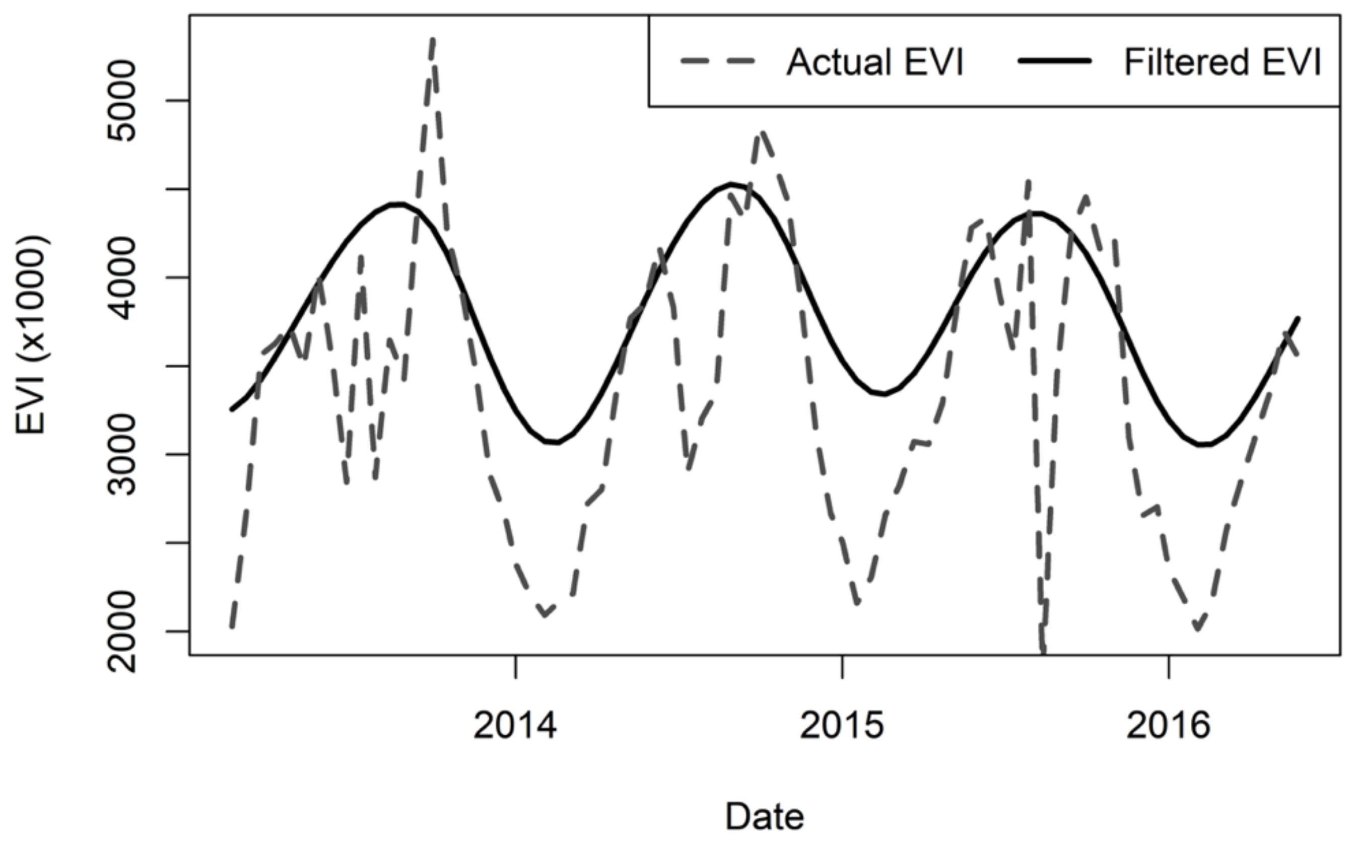
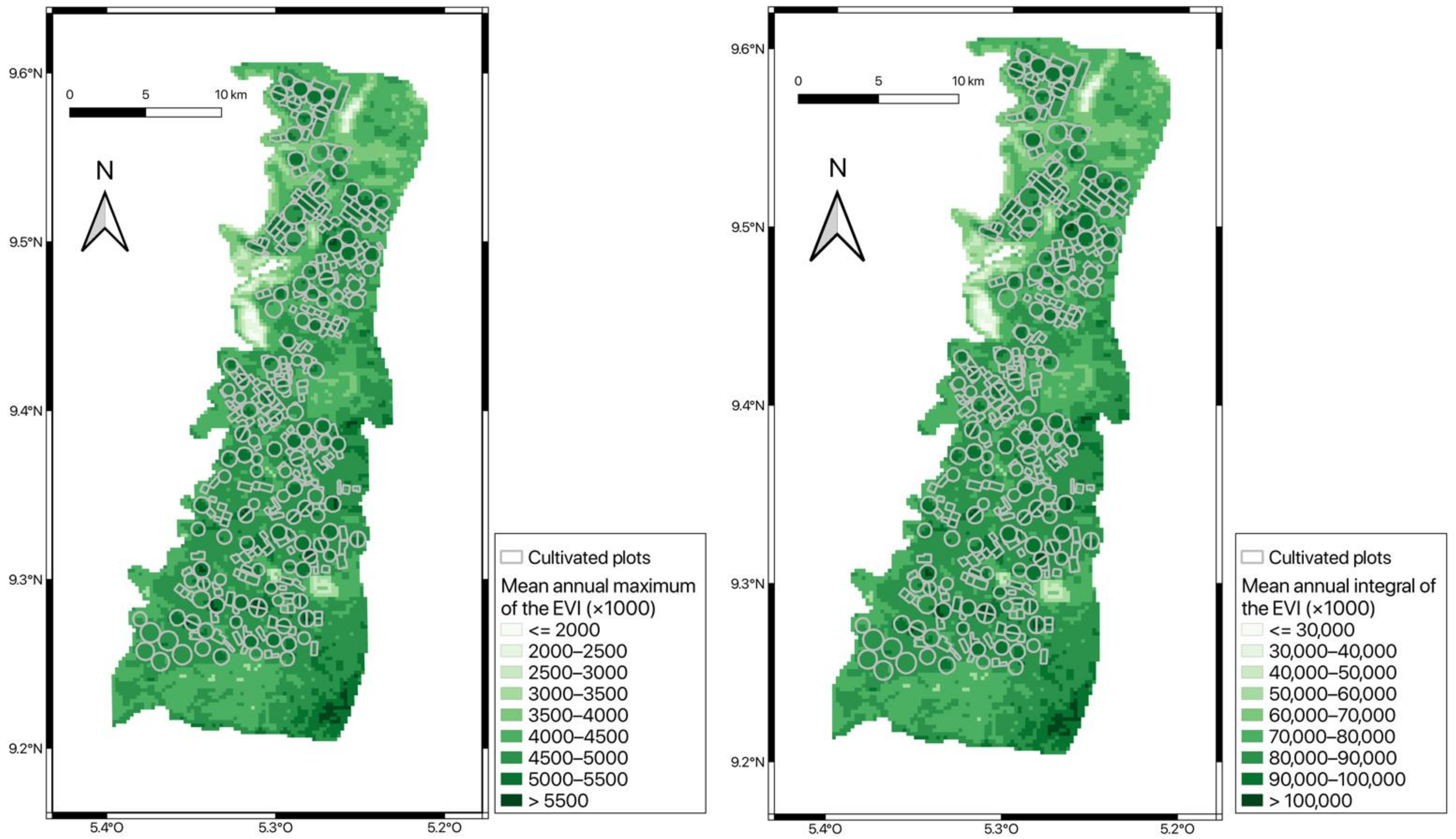
3.2.3. Forecasting from Satellite Variables at the Plot Level

The exact spatial location of the plots was only available for the Ferké 2 area and for the harvest campaigns from 2011 to 2020. Therefore, the analysis will be restricted to this zone and to these years.

Explanatory Model

For each plot, the NDVI and EVI were taken as respectively equal to the mean filtered value of the set of pixels (250-m square) intercepting the geometry of the plot. The correlation between sugarcane yields and the maximum value of NDVI and EVI on the one hand, and the integral of NDVI and EVI over the whole year on the other hand, was then computed.

Forecasting Model

As in the first model, the forecasting model consists of training a random forest algorithm on the set of different years of the tested year, and makes a prediction for the tested year. The variables used to train this algorithm were the cropping practices and the satellite index restricted to the month of the prediction.

3.3. Comparison of the Models

In order to compare the different forecasting models, yields were classified into three terciles: low yield, medium yield and high yield. The ability of each forecasting model to place the yields in the correct category was then observed through a confusion matrix.

Three complementary metrics, not relying on prevalence, were then used to evaluate the performance of this classification. There are often used to assess prediction models of classification [55]: (i) accuracy, which measures the proportion of the correct forecast; (ii) sensitivity (the proportion of correctly identified points in a class); and (iii) specificity (the proportion of points correctly identified as not belonging to a class). In our case, the accuracy of the model measures its overall ability to correctly classify yields. The sensitivity of the high and low classes measures the model’s ability to detect years with high or low yields. The specificity of these classes measures the model’s ability not to consider the year’s yields to be high or low when they are not.

4. Results and Discussion

4.1. Trends and Change-Points in Data

Table 4. Trends and change-points observed in the data used in this study.

Indices	Change-Points	Trends
Rainfall data
PRECTOT	No change-point	No trend
SPI12	No change-point	No trend
Temperature data
Tmoy	No change-point	Significant increasing trend at the 1% threshold in Ferké 1 and 2
Tmin	No change-point	Significant increasing trend at the 5% threshold in Ferké 1 and 2
Tmax	No change-point	Significant increasing trend at the 5% threshold in Ferké 1 and 2
Sugarcane yields
Yields	No change-point	No trend

shows all of the trends and change-points observed in our data. No change-point was observed for all the different indices of rainfall. Regarding sugarcane yields, no trend was observed, as highlighted by Figure 4. There are significant increasing trends at the 5% threshold for Tmin and Tmax in Ferké 1 and 2 and at the 1% threshold for Tmoy in Ferké 1 and 2, these trends can be observed in Figure 5. For these indices, the Sen’s slope is between 0.1 °C and 0.2 °C per year.

Several studies have analyzed extreme rains and droughts in West Africa. These studies used data over longer periods than ours (at least 50 years). However, the data used here have the advantage of being more recent, coming directly from rainfall stations and having a high spatial density. In agreement with Sacré Regis M. et al. [56], who investigated changes in precipitation during the last 30 years using the CHIRPS dataset (blending satellite products and rain gauge data), no significant trend of precipitation was found in our study area.

Regarding temperature, statistically significant warming in Africa is considered to be evident in the literature [57,58,59]. Nevertheless, Barry et al. [57] calculated an increase in the annual maximum temperature of 0.27 °C per decade from 1981 to 2010 and an increase in the annual minimum temperature of 0.22 °C per decade on the same period, whereas in this study, an increase in both minimum and maximum temperature of approximately 1 °C per decade was found. This higher warming rate may be due to the shorter period of our study. Broadly speaking, the main limitation of this analysis is the sort period of data availability, which can lead to high imprecision in the trend level.

4.2. Explanatory and Yield-Forecasting Models

In this section, the results of the three different statistical models introduced in the Methodology are shown. First, the correlation between yields and a set of variables are computed (explanatory model) and then, a test of forecasting yields for a specific year is performed (forecasting model). In that case, we consider the data available only before a particular month. The model is trained on all but one year, on which we will try to forecast yields values; the process is repeated to predict yields for all years.

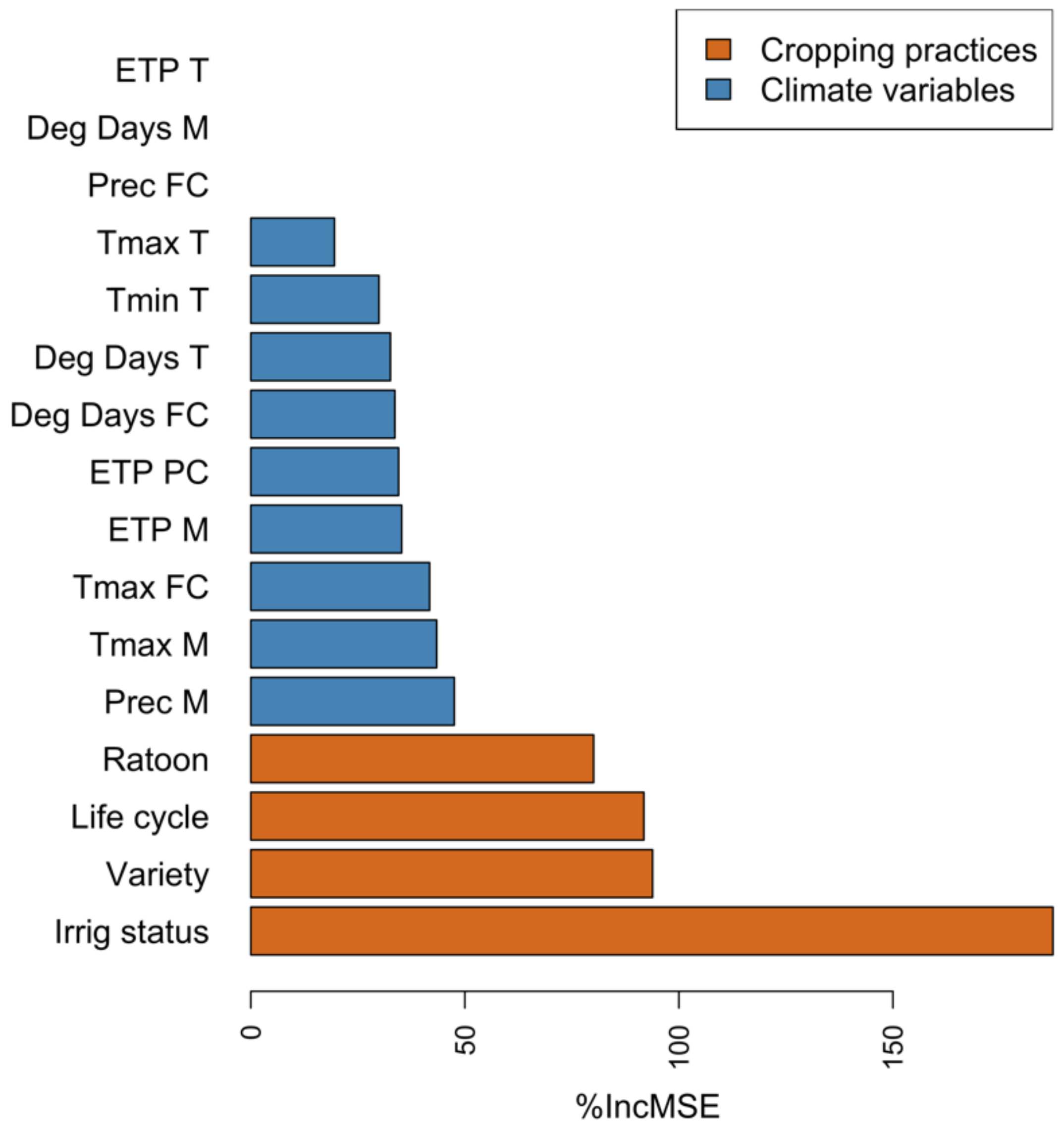
4.2.1. Explanatory and Forecasting Models Using Climate Variables and Cropping Practices at the Plot Scale

Explanatory Model

Table 5. Result of the stepwise regression for yields in tons of sugarcane per hectare in Ferké zones 1 and 2 from 2008 to 2020.

	Sugarcane Yields
	Coefficient	p-Value
Prec in maturation phase	0.0481 ***	(0.0000)
Prec in pre-growth phase	−0.0139 ***	(0.0001)
Max temp in high growth phase	−3.2336 ***	(0.0000)
Max temp in maturation phase	−1.3556 ***	(0.0000)
Max temp in pre-growth phase	1.5727 ***	(0.0000)
N	5097
R2 (cropping practices)	0.5114
R2 (all variables)	0.5413

*** p < 0.001. Prec = precipitation, Temp = temperature, Max = maximum. R² (cropping practices) is the adjusted coefficient of determination for the model including only the cropping practices. R² (all variables) is the adjusted coefficient of determination for the model including the cropping practices’ variables and the climate variables shown in the table.

shows the stepwise model based on the plot-level regression of yields as a function of climate variables and cropping practices. The cropping practices included in the model are irrigation status, sugarcane variety, month of harvest, number of plant regrowth and length of life cycle. They are all significant at the 1% threshold and are not represented in the table. The model has variance inflation factors of less than 10 for all variables, which justifies the absence of multicollinearity. The model with the lowest Mallow Cp value has been selected, to keep the variables with the most significant relation with sugarcane yields. This model is not necessarily optimal; however, it is not far from it and can be used to draw interesting conclusions on the capacity of meteorological variables to explain variations in sugarcane yields at plot levels.

As a main result, cropping practices explain 51% of the yields at the plot scale and adding climate variables into the model increases the coefficient of determination by only 3%. Thus, cropping practices play a greater part in explaining yields at the plot level than climate variables.

A relationship between rainfall and yields is often observed [60,61] but the model using the combination of rainfall and maximum temperature demonstrated the best performance in explaining the variations of sugarcane yields.

Table 5 shows that during the pre-growth phase, rainfall negatively affects yields. Binbol et al. [47] and Humbert [30] also found that during the pre-growth phase, too much rainfall can affect plant development, especially when drainage is inefficient. Besides, the accumulated rainfall during the maturation period has the heaviest effect on yields. However, in this study, the relationship may be amplified when comparing the particularly wet year 2015 with the high accumulated rainfall during the ripening phase and the high yields of the same year, mainly due to good cropping practices. Indeed, according to SUCAF, irrigation management was particularly good that year, and the implementation of a new weeding method was very effective [62].

Maximum temperature also appears in some studies to be a good proxy of yields [51,63]. While increasing the maximum temperature is often considered beneficial for sugarcane yields [30,32,64], Deressa et al. [31] consider that temperatures above 35 °C can negatively affect plant growth. However, at Ferké 1 and 2, the average temperatures of the warmest month have always been above 35 °C between 2007 and 2019, and had reached 38 °C in some years. Then the negative coefficient linked to maximum temperature during the high-growth phase may be due to this quadratic relation between yields and maximum temperature.

Forecasting Model

Figure 6 describes the values forecasted by the algorithm compared to the actual values. An average coefficient of determination for each forecast equal to 0.51 and an RMSE value equal to 14.28 tons per hectare was obtained. These results show that the forecasted values have a smaller standard deviation than the actual values, meaning that the algorithm was not able to detect conditions leading to extreme yield values.

Cropping Practices

The model with cropping variables explained 51% of yields at the plot scale, whereas considering only the climate variables, any model tested can explain around 10% of the yields. Adding climate variables to the model with cropping variables allows an increase of only 0.03 in the coefficient of determination to explain yields. This confirms the importance of information on cropping practices at the plot level and in the random forest model, Figure 7 shows that the importance of cropping practices greatly exceeds that of the climate variables.

Thus, the climate variables provide little additional information to explain the variations in yields at the sugarcane plot level. Unrecorded cropping practices such as herbicides and fertilizers or planting and harvesting methods also have effects at the plot level. They can induce noise on yield values and, therefore, do not allow the statistical effect of climate variables to be properly observed.

Cropping practices frequently depend on the studies carried out. For example, irrigation status, which is the most important variable in our model (Figure 7), was never present in the previous studies because all plots studied were either irrigated or rainfed. Therefore, it is difficult to compare the effect and relative importance of irrigation practice found in this study with previous studies. However, the number of new plant regrowth is a cropping practice that is often taken into account because its effect on yield reduction is well known [65]. Bocca and Rodrigues [60] and Hammer et al. [24] found that the importance of this variable greatly surpassed climate variables in all of their models. Similarly, according to Ferraro et al. [66], cropping practices such as the farm, the variety, the life cycle length, the month of harvest and the geographic characteristics had a greater effect on yields than climate variables.

Nevertheless, cropping practices, especially those that do not depend on the biological characteristics of the plant (variety, number of regrowth, etc.), are local, and are inherently dependent on crop management. It is possible that in areas where management is standardized and industrialized, these cultural practices will have a weak effect. For example, in the model developed by Oliveira et al. [25] in Brazil, where sugarcane production is more standardized and industrialized than in Ivory Coast, the importance of meteorological variables outweighs those due to cropping practices.

In Ferké 1 and 2, cropping practices have clearly significant effects on yields. One of the limitations of our database is that it does not take into account some practices that, according to the SUCAF, have an influence on sugarcane yields. These include the use of the slash-and-burn method, weeding methods or good irrigation management. This lack of information accentuates the noise caused by cropping practices on yield values and makes it difficult to measure the effect of climate on these yields.

4.2.2. Explanatory and Forecasting Models Using Climate Data at the Scale of Ferké 1 and Ferké 2

Explanatory Model

The stepwise regression model showed that the most efficient model was the one which explained the yields based on the average minimum temperature during the year. This model explained 38% of the yields and this relationship was significant at the 1% threshold (

Table 6. Result of stepwise regression for sugarcane yields in tons per hectare and sugar content in percentage in Ferké 1 and 2.

	Sugarcane Yields (T/Ha)
	Coefficient	p-Value
(Intercept)	−37.68	(0.23)
Minimal temperature	5.33 **	(0.00)
N	24
R2	0.38

** p < 0.01.

). Figure 8 shows the relationship between yields and minimal temperature at the zone level.

In order to observe more precisely the influence of the minimum temperature on yields, four phases were studied: the tillering phase from January to March, the pre-growth phase from April to May, the high-growth phase from June to October and the ripening phase from November to December.

When analyzing the relation between minimum temperature and yields during these four phases, the minimum temperature during the tillering and the pre-growth phase explained the yield variations more significantly. Although Greenland [67] and Saithanu et al. [61] also found the positive effect of minimum temperature on yields during the year, Samui et al. [68] and Shrivastava [69] even observed that minimum temperature particularly influenced yields during the first three months after harvest, and thus during the tillering and pre-growth phases. During these phases, sugarcane does not tolerate extreme temperatures and needs high temperatures [30]. Our study confirms that in Ferké 1 and 2, minimum temperature is a key climate driver of the sugarcane yields especially during the pre-growth and the tillering phases.

Forecasting Model

Figure 9 shows the results of the forecasting model. The minimum temperature during the tillering and pre-growth period is able to forecast 23% of the yield variability over the year studied. Thus, this model forecasts the yields as soon as the month of May, i.e., four months before the beginning of the harvest.

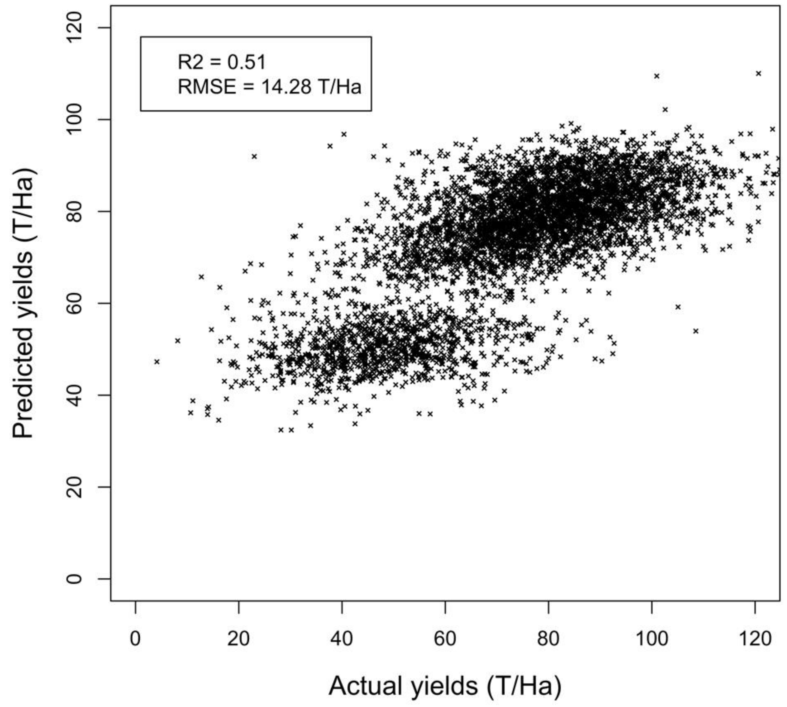
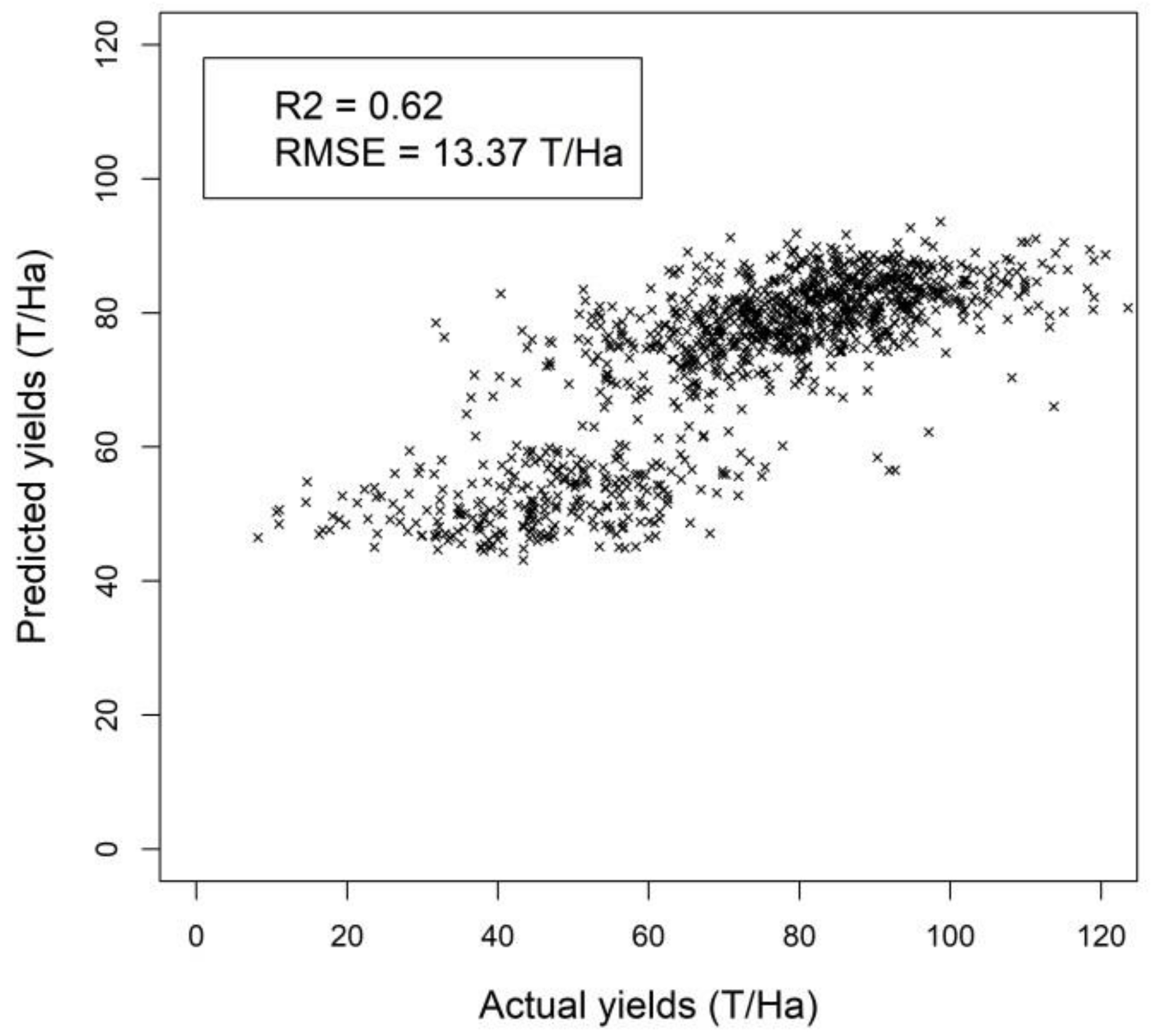
4.2.3. Explanatory and Forecasting Models Using Satellite Data

Explanatory Model

Table 7. Regression results between yields and integral of NDVI (Int_NDVI), annual maximum value of NDVI (Max_NDVI), integral of EVI (Int_EVI) and annual maximum value of EVI (Max_EVI).

	p-Value	R2	RMSE
Int_NDVI	<2.10−16	0.35	17.19
Max_NDVI	<2.10−16	0.16	19.57
Int_EVI	<2.10−16	0.43	14.31
Max_EVI	<2.10−16	0.31	15.67

R² is the coefficient of determination.

details the result of the regressions of sugarcane yields according to the annual maximum of the NDVI, the NDVI integrated over the year, the annual maximum of the EVI and the EVI integrated over the year. The simple equation estimated is:

$${\mathrm{Y}}_{\mathrm{it}}=\mathsf{\alpha }+{\mathsf{\beta }\mathrm{VI}}_{\mathrm{it}}+{\mathsf{\epsilon }}_{\mathrm{it}}$$

(6)

where Y_it is the yield value for the plot i at the year t, VI_it is the value of the vegetation index and ${\mathsf{\epsilon }}_{\mathrm{it}}$ is the classical error term. The four relationships are significant (p-value < 0.001) and explain 16%, 35%, 31% and 41% of sugarcane yields, respectively.

The integrals of the vegetation indices were more effective in explaining yield variations than the maximum of these indices. This is consistent with observations made by Bégué et al. [26]. In addition, the integrated EVI is slightly better at explaining yields than the integrated NDVI. Son et al. [70] also found in their study on rice yield prediction that, while both relationships are highly significant, switching from NDVI to EVI allows a slight increase in the coefficient of determination.

Forecasting Model

When the integral of EVI is limited to a previous month, the decrease in the coefficient of determination is about 1% per month. After consultation with local experts, we consider the integral of the EVI from January to August in our forecasting model. This single variable explains 38% of the sugarcane yields at Ferké 2 between 2011 and 2020 with a high level of significance.

Figure 10 describes the yields forecasted by the algorithm versus the actual yields for each year, after training a random forest regression algorithm over all other years and using the integral of EVI from January to August and the information on cropping practices. This model forecasts yields with a coefficient of determination of 62% and a RMSE equal to 13.37 tons per hectare. The standard deviation of the forecasted values is small compared to the actual values. Therefore, the algorithm is not able to forecast extreme yield values.

4.3. Overall Assessment of the Forecasting Models

Table 8. Confusion matrix for forecasted and actual yields for the different forecasting models studied; note that values for the bottom table (with EVI) are for Ferké 2 only.

	Cropping Practices and Climate Variables at the Plot Level (Accuracy = 58%)
	Yields	Forecast
		High	Medium	Low
Observed	High	756	926	16
	Medium	358	1225	115
	Low	68	620	1011
	Climate variables averaged at the zone level (accuracy = 54%)
	Yields	Forecast
		High	Medium	Low
Observed	High	7	1	0
	Medium	4	2	2
	Low	0	4	4
	Cropping practices and integral of the EVI from January to August (accuracy = 65%)
	Yields	Forecast
		High	Medium	Low
Observed	High	190	184	4
	Medium	66	293	18
	Low	7	112	259

shows the results of the categorization of yields after the application of the forecast algorithm for each year trained on all the other years. The metric used was the accuracy, which measures the percentage of correct classifications. The model using the integral of EVI was found to be more accurate with 65% of the correct classification.

Table 9. Sensibility and specificity for high, medium and low sugarcane yields for the 3 forecasting models studied.

Models	Indices	Sugarcane Yields
		High	Medium	Low
Climate variables at the scale of Ferké 1/Ferké 2 (Section 3.2.2)	Sensitivity	88%	25%	50%
	Specificity	75%	69%	88%
Cropping practices and climate variables at the plot scale (Section 3.2.1)	Sensitivity	45%	72%	60%
	Specificity	87%	54%	96%
Cropping practices and integral of the EVI from January to August (Section 3.2.3)	Sensitivity	50%	78%	69%
	Specificity	90%	61%	98%

shows the sensitivity and specificity for each yield category and for each model.

All models have important specificities for both low and high classes. This means that they will rarely forecast that yields are low or high if they are not. The sensitivity for these same classes is relatively low for both models at the plot level; the algorithm will most often forecast average yields.

From an operational point of view, the models should particularly avoid making errors on high and low yields, i.e., they must have a high sensitivity for these classes. Indeed, if the algorithm wrongly forecasts high yields for a specific year, it will have a high cost for the producer. The producer would have anticipated high yields and prepared for this (through the recruitment of additional farmers, investments due to a high-revenue year) and these costs would be useless. On the other hand, if a high yield year is not detected, and is considered as average, this simply makes the model inefficient and does not cause any additional cost.

The model that performed best was the one using the integral of the EVI from January to August and the cropping practices. This one showed greater accuracy and had a high specificity for the low and high classes: in only 2% of cases and 10% of cases, it forecasted that yields were respectively low and high when this was not the case. Moreover, its sensitivity was acceptable for the low class: it detected low yields in 69% of cases. It was, on the other hand, less efficient in detecting high yields; it detected them in 50% of cases.

5. Conclusions

The vulnerability of the African agricultural sector to climate change is a threat that requires the implementation of adaptation strategies. Climate services are part of these adaptation strategies in helping stakeholders of the agricultural sector to make decisions. According to the assessment carried out on Nationally Determined Contributions by the FAO and WMO, 85% of countries (100/117) identified “climate services” as being a fundamental element for planning and decision-making in the area of agriculture and food security [14].

In this context, the development of models for forecasting sugarcane yields could enable producers to improve crop management and to anticipate years that are more or less good in terms of climate variables and yields. In addition, such a study can inform the national weather service (Sodexam) on the most relevant variables to be forecasted and the appropriate climate products to deliver to meet the needs of sugarcane producers.

First, our analysis of rainfall data in our study area showed that despite positive coefficients of Sen for most of the rainfall stations, there was no significant trend in the evolution of accumulated rainfall and drought years. Regarding temperature, a significant trend was observed for the minimal, the maximal and the mean temperature in Ferké 1 and 2 at the 5% threshold. The warming trend was approximately 1 °C per decade for all the indices.

Then, the study of different forecasting models showed (i) that using only climate variables enabled us to forecast future yields with moderate performance (R² = 0.23 using minimal temperature) and (ii) that using satellite variables provided better results. The integral of a well-known satellite index (EVI), over the year contributed to explaining 43% of the year-to-year variability of yields. The resulting forecasting model allowed the correct categorization of 60% of the yields. This model can detect high or low yields in 50% and 69% of cases, respectively, while being wrong in only 10% and 2% of cases, respectively. However, it should be noted that these results only consider the Ferké 2 area from 2011 to 2020. It would be necessary to validate these results over a longer period.

The improvement of this model would henceforth require the use of more precise satellite images. Although MODIS data have the advantage of being easily accessible and free of charge, the resolution of 250 m leads to an overlap of several plots by a single pixel. Providing images at a resolution of 30 m, for example, could be an important source of improvement in the accuracy of our model. These modeling results from the “agro-climatic” Work Package of the CLIMSUCAF project will now have to be compared with those of the “socio-economic” Work Package, which aims to question sugarcane growers, owners of rainfed plots and SUCAF managers of irrigated plots on (i) the sensitivity of their crops to climate variables, and (ii) their needs in terms of weather and climate information for more resilient management and sustainable exploitation of sugarcane. The results of this study will notably help to guide surveys and discussions with local stakeholders, and the results of the surveys will in return help to refine the models, taking into account parameters that had not previously appeared relevant.

References

1. World Bank. Agriculture, Forestry, and Fishing, Value Added (% of GDP)—Cote d’Ivoire. Available online: https://data.worldbank.org/indicator/NV.AGR.TOTL.ZS?locations=CI (accessed on 7 September 2020).
2. FAO. World Food and Agriculture—Statistical Pocketbook 2019; Food & Agriculture Organization: Rome, Italy, 2019; ISBN 978-92-5-131849-2. [Google Scholar]
3. Ransinghe, R.; Ruane, A.C.; Vautard, R.; Arnell, N.; Coppola, E.; Cruz, F.A.; Dessai, S.; Islam, A.S.; Rahimi, M.; Carrascal, D.R.; et al. Climate Change Information for Regional Impact and for Risk Assessment. In Climate Change 2021: The Physical Science Basis. Contribution of Working Group I to the Sixth Assessment Report of the Intergovernmental Panel on Climate Change; Masson Delmotte, V., Zhai, P., Pirani, A., Connors, S.L., Péan, C., Berger, S., Caud, N., Chen, Y., Goldfarb, L., Gomis, M.I., Eds.; IPCC: Geneva, Switzerland; Cambridge University Press: Cambridge, UK, 2021; In Press. [Google Scholar]
4. Konan, E.A.; Pene, C.B.; Dick, E. Caractérisation Agro-Climatique Du Périmètre Sucrier de Ferké 2 Au Nord de La Côte d’Ivoire. J. Appl. Biosci. 2017, 116, 11532–11545. [Google Scholar] [CrossRef] [Green Version]
5. Noufé, D.; Mahé, G.; Kamagaté, B.; Servat, É.; Tié, A.G.B.; Savané, I. Climate Change Impact on Agricultural Production: The Case of Comoe River Basin in Ivory Coast. Hydrol. Sci. J. 2015, 60, 1972–1983. [Google Scholar] [CrossRef] [Green Version]
6. Sanogo, S.; Fink, A.H.; Omotosho, J.A.; Ba, A.; Redl, R.; Ermert, V. Spatio-Temporal Characteristics of the Recent Rainfall Recovery in West Africa. Int. J. Climatol. 2015, 35, 4589–4605. [Google Scholar] [CrossRef]
7. Sultan, B.; Defrance, D.; Iizumi, T. Evidence of Crop Production Losses in West Africa Due to Historical Global Warming in Two Crop Models. Sci. Rep. 2019, 9, 12834. [Google Scholar] [CrossRef] [Green Version]
8. Parkes, B.; Defrance, D.; Sultan, B.; Ciais, P.; Wang, X. Projected Changes in Crop Yield Mean and Variability over West Africa in a World 1.5 K Warmer than the Pre-Industrial Era. Earth Syst. Dyn. 2018, 9, 119–134. [Google Scholar] [CrossRef] [Green Version]
9. Marin, F.R.; Jones, J.W.; Singels, A.; Royce, F.; Assad, E.D.; Pellegrino, G.Q.; Justino, F. Climate Change Impacts on Sugarcane Attainable Yield in Southern Brazil. Clim. Chang. 2013, 117, 227–239. [Google Scholar] [CrossRef] [Green Version]
10. Singels, A.; Jones, M.; Marin, F.; Ruane, A.; Thorburn, P. Predicting Climate Change Impacts on Sugarcane Production at Sites in Australia, Brazil and South Africa Using the Canegro Model. Sugar Tech 2014, 16, 347–355. [Google Scholar] [CrossRef]
11. Linnenluecke, M.K.; Nucifora, N.; Thompson, N. Implications of Climate Change for the Sugarcane Industry. WIREs Clim. Chang. 2018, 9, e498. [Google Scholar] [CrossRef]
12. Zhao, D.; Li, Y.-R. Climate Change and Sugarcane Production: Potential Impact and Mitigation Strategies. Int. J. Agron. 2015, 2015, e547386. [Google Scholar] [CrossRef] [Green Version]
13. Vaughan, C.; Muth, M.F.; Brown, D.P. Evaluation of Regional Climate Services: Learning from Seasonal-Scale Examples across the Americas. Clim. Serv. 2019, 15, 100104. [Google Scholar] [CrossRef]
14. World Meteorological Organization. 2019 State of Climate Services; World Meteorological Organization: Geneva, Switzerland, 2019; p. 44. [Google Scholar]
15. Vaughan, C.; Dessai, S. Climate Services for Society: Origins, Institutional Arrangements, and Design Elements for an Evaluation Framework. Wiley Interdiscip. Rev. Clim. Chang. 2014, 5, 587–603. [Google Scholar] [CrossRef] [PubMed]
16. Akwango, D.; Obaa, B.B.; Turyahabwe, N.; Baguma, Y.; Egeru, A. Effect of Drought Early Warning System on Household Food Security in Karamoja Subregion, Uganda. Agric. Food Secur. 2017, 6, 43. [Google Scholar] [CrossRef]
17. Ouedraogo, M.; Zougmore, R.; Barry, S.; Some, L. The Value and Benefits of Using Seasonal Climate Forecasts in Agriculture: Evidence from Cowpea and Sesame Sectors in Climate-Smart Villages of Burkina Faso (Info Note, pp. 1–4). Available online: https://www.researchgate.net/publication/292987809_The_value_and_benefits_of_using_seasonal_climate_forecasts_in_agriculture_evidence_from_cowpea_and_sesame_sectors_in_climate-smart_villages_of_Burkina_Faso (accessed on 29 September 2020).
18. Vaughan, C.; Hansen, J.; Roudier, P.; Watkiss, P.; Carr, E. Evaluating Agricultural Weather and Climate Services in Africa: Evidence, Methods, and a Learning Agenda. WIREs Clim. Chang. 2019, 10, e586. [Google Scholar] [CrossRef] [Green Version]
19. Keating, B.A.; Robertson, M.J.; Muchow, R.C.; Huth, N.I. Modelling Sugarcane Production Systems I. Development and Performance of the Sugarcane Module. Field Crops Res. 1999, 61, 253–271. [Google Scholar] [CrossRef]
20. Singels, A.; Donaldson, R.A. A Simple Model of Unstressed Sugarcane Canopy Development. Proc. S. Afr. Sug. Technol. Ass. 2000, 74, 151–154. [Google Scholar]
21. Cardozo, N.P.; Sentelhas, P.C. Climatic Effects on Sugarcane Ripening under the Influence of Cultivars and Crop Age. Sci. Agric. 2013, 70, 449–456. [Google Scholar] [CrossRef] [Green Version]
22. Scarpari, M.S.; de Beauclair, E.G.F. Physiological Model to Estimate the Maturity of Sugarcane. Sci. Agric. 2009, 66, 622–628. [Google Scholar] [CrossRef] [Green Version]
23. Everingham, Y.; Sexton, J.; Skocaj, D.; Inman-Bamber, G. Accurate Prediction of Sugarcane Yield Using a Random Forest Algorithm. Agron. Sustain. Dev. 2016, 36, 27. [Google Scholar] [CrossRef] [Green Version]
24. Hammer, R.G.; Sentelhas, P.C.; Mariano, J.C.Q. Sugarcane Yield Prediction through Data Mining and Crop Simulation Models. Sugar Tech 2020, 22, 216–225. [Google Scholar] [CrossRef]
25. De Oliveira, M.P.G.; Bocca, F.F.; Rodrigues, L.H.A. From Spreadsheets to Sugar Content Modeling: A Data Mining Approach. Comput. Electron. Agric. 2017, 132, 14–20. [Google Scholar] [CrossRef]
26. Bégué, A.; Todoroff, P.; Pater, J. Multi-Time Scale Analysis of Sugarcane within-Field Variability: Improved Crop Diagnosis Using Satellite Time Series? Precis. Agric. 2008, 9, 161–171. [Google Scholar] [CrossRef]
27. Robson, A. Developing Sugarcane Yield Prediction Algorithms from Satellite Imagery. In Proceedings of the 34th Conference of the Australian Society of Sugar Cane Technologists, Cairns, Australia, 1–4 May 2012; Volume 34, p. 11. [Google Scholar]
28. Albergel, J.; Lévêque, C.; Aubertin, C. Le nord de la Côte d’Ivoire, un milieu approprié aux aménagements de petite et moyenne hydraulique. In L’eau en Partage: Les Petits Barrages de Côte d’Ivoire; Cecchi, P., Ed.; Latitudes 23; IRD: Paris, France, 2007; pp. 45–57. [Google Scholar]
29. Gaudin, R. Incidence de l’eau sur la culture de la canne. Agric. Dév. 1999, 24, 5–8. [Google Scholar]
30. Humbert, R.P. The Growing of Sugar Cane; Elsevier Pub. Co.: Amsterdam, The Netherlands; New York, NY, USA, 1968. [Google Scholar]
31. Deressa, T.; Hassan, R.; Poonyth, D. Measuring the Impact of Climate Change on South African Agriculture: The Case of Sugarcane Growing Regions. Agrekon 2005, 44, 524–542. [Google Scholar] [CrossRef] [Green Version]
32. Hunsigi, G. Production of Sugarcane: Theory and Practice; Springer Science & Business Media: Berlin/Heidelberg, Germany, 2012; ISBN 978-3-642-78133-9. [Google Scholar]
33. Dias, H.B.; Sentelhas, P.C. Evaluation of Three Sugarcane Simulation Models and Their Ensemble for Yield Estimation in Commercially Managed Fields. Field Crops Res. 2017, 213, 174–185. [Google Scholar] [CrossRef]
34. Funk, C.; Peterson, P.; Landsfeld, M.; Pedreros, D.; Verdin, J.; Shukla, S.; Husak, G.; Rowland, J.; Harrison, L.; Hoell, A.; et al. The Climate Hazards Infrared Precipitation with Stations—A New Environmental Record for Monitoring Extremes. Sci. Data 2015, 2, 150066. [Google Scholar] [CrossRef] [Green Version]
35. Romero, R.; Guijarro, J.A.; Ramis, C.; Alonso, S. A 30-Year (1964–1993) Daily Rainfall Data Base for the Spanish Mediterranean Regions: First Exploratory. Int. J. Clim. 1998, 18, 541–560. [Google Scholar] [CrossRef]
36. Teegavarapu, R.S.V.; Chandramouli, V. Improved Weighting Methods, Deterministic and Stochastic Data-Driven Models for Estimation of Missing Precipitation Records. J. Hydrol. 2005, 312, 191–206. [Google Scholar] [CrossRef]
37. Weier, J.; Herring, D. Measuring Vegetation (NDVI and EVI); NASA Earth Observatory: Washington, DC, USA.
38. Didan, K.; Munoz, A.B.; Huete, A. MODIS Vegetation Index User’s Guide (MOD13 Series); Vegetation Index and Phenology Lab, University of Arizona: Tucson, AZ, USA, 2015; p. 35. [Google Scholar]
39. Fernandes, J.L.; Ebecken, N.F.F.; Esquerdo, J.C.D.M. Sugarcane Yield Prediction in Brazil Using NDVI Time Series and Neural Networks Ensemble. Int. J. Remote Sens. 2017, 38, 4631–4644. [Google Scholar] [CrossRef]
40. Dubey, S.K.; Gavli, A.S.; Yadav, S.K.; Sehgal, S.; Ray, S.S. Remote Sensing-Based Yield Forecasting for Sugarcane (Saccharum officinarum L.) Crop in India. J. Indian Soc. Remote Sens. 2018, 46, 1823–1833. [Google Scholar] [CrossRef]
41. Shao, Y.; Lunetta, R.S.; Wheeler, B.; Iiames, J.S.; Campbell, J.B. An Evaluation of Time-Series Smoothing Algorithms for Land-Cover Classifications Using MODIS-NDVI Multi-Temporal Data. Remote Sens. Environ. 2016, 174, 258–265. [Google Scholar] [CrossRef]
42. Kandasamy, S.; Baret, F.; Verger, A.; Neveux, P.; Weiss, M. A Comparison of Methods for Smoothing and Gap Filling Time Series of Remote Sensing Observations—Application to MODIS LAI Products. Biogeosciences 2013, 10, 4055–4071. [Google Scholar] [CrossRef] [Green Version]
43. Klisch, A.; Atzberger, C. Operational Drought Monitoring in Kenya Using MODIS NDVI Time Series. Remote Sens. 2016, 8, 267. [Google Scholar] [CrossRef] [Green Version]
44. McKee, T.B.; Doesken, N.J.; Kleist, J. The Relationship of Drought Frequency and Duration to Time Scales. In Proceedings of the 8th Conference on Applied Climatology, Anaheim, CA, USA, 17–22 January 1993; p. 6. [Google Scholar]
45. Debortoli, N.; Dubreuil, V.; Heinke, C.; Filho, S.R. Tendances et ruptures des séries pluviométriques dans la région méridionale de l’Amazonie brésilienne. In 25e Colloque de l’AIC; Université Joseph Fourier: Grenoble, French, 2012; pp. 201–206. [Google Scholar]
46. Soro, G.; Noufé, D.; Goula Bi, T.; Shorohou, B. Trend Analysis for Extreme Rainfall at Sub-Daily and Daily Timescales in Côte d’Ivoire. Climate 2016, 4, 37. [Google Scholar] [CrossRef] [Green Version]
47. Binbol, N.; Adebayo, A.; Kwon-Ndung, E. Influence of Climatic Factors on the Growth and Yield of Sugar Cane at Numan, Nigeria. Clim. Res. 2006, 32, 247–252. [Google Scholar] [CrossRef] [Green Version]
48. Skocaj, D.M.; Everingham, Y.L. Identifying Climate Variables Having the Greatest Influence on Sugarcane Yields in the Tully Mill Area. In Proceedings of the Australian Society of Sugar Cane Technologists; Bruce, R.C., Ed.; Australian Society of Sugar Cane Technologists: Mackay, Australia, 2014; Volume 36, pp. 53–61. [Google Scholar]
49. Bégué, A.; Lebourgeois, V.; Bappel, E.; Todoroff, P.; Pellegrino, A.; Baillarin, F.; Siegmund, B. Spatio-Temporal Variability of Sugarcane Fields and Recommendations for Yield Forecast Using NDVI. Int. J. Remote Sens. 2010, 31, 5391–5407. [Google Scholar] [CrossRef] [Green Version]
50. Kutner, M.H. Applied Linear Statistical Models, 5th ed.; The McGraw-Hill/Irwin Series Operations and Decision Sciences; McGraw-Hill Irwin: Boston, MA, USA, 2005; ISBN 978-0-07-238688-2. [Google Scholar]
51. Saithanu, K.; Mekparyup, J. Forecasting Sugar Cane Yield in the Northeast of Thailand with MLP Models. Glob. J. Pure Appl. Math. 2015, 11, 2161–2164. [Google Scholar]
52. Breiman, L. Random Forests. Mach. Learn. 2001, 45, 5–32. [Google Scholar] [CrossRef] [Green Version]
53. Liaw, A.; Wiener, M. Classification and Regression by RandomForest. R News 2002, 2, 18–22. [Google Scholar]
54. Ferraciolli, M.A.; Bocca, F.F.; Rodrigues, L.H.A. Neglecting Spatial Autocorrelation Causes Underestimation of the Error of Sugarcane Yield Models. Comput. Electron. Agric. 2019, 161, 233–240. [Google Scholar] [CrossRef]
55. Beguería, S. Validation and Evaluation of Predictive Models in Hazard Assessment and Risk Management. Nat. Hazards 2006, 37, 315–329. [Google Scholar] [CrossRef] [Green Version]
56. Sacré Regis, M.D.; Mouhamed, L.; Kouakou, K.; Adeline, B.; Arona, D.; Koffi Claude, A.K.; Talnan Jean, H.C.; Salomon, O.; Issiaka, S. Using the CHIRPS Dataset to Investigate Historical Changes in Precipitation Extremes in West Africa. Climate 2020, 8, 84. [Google Scholar] [CrossRef]
57. Barry, A.A.; Caesar, J.; Klein Tank, A.M.G.; Aguilar, E.; McSweeney, C.; Cyrille, A.M.; Nikiema, M.P.; Narcisse, K.B.; Sima, F.; Stafford, G.; et al. West Africa Climate Extremes and Climate Change Indices: West Africa Climate Extremes. Int. J. Climatol. 2018, 38, e921–e938. [Google Scholar] [CrossRef]
58. Kruger, A.C.; Sekele, S.S. Trends in Extreme Temperature Indices in South Africa: 1962–2009. Int. J. Climatol. 2013, 33, 661–676. [Google Scholar] [CrossRef]
59. Vincent, L.A.; Aguilar, E.; Saindou, M.; Hassane, A.F.; Jumaux, G.; Roy, D.; Booneeady, P.; Virasami, R.; Randriamarolaza, L.Y.A.; Faniriantsoa, F.R.; et al. Observed Trends in Indices of Daily and Extreme Temperature and Precipitation for the Countries of the Western Indian Ocean, 1961–2008. J. Geophys. Res. Atmos. 2011, 116. [Google Scholar] [CrossRef]
60. Bocca, F.F.; Rodrigues, L.H.A. The Effect of Tuning, Feature Engineering, and Feature Selection in Data Mining Applied to Rainfed Sugarcane Yield Modelling. Comput. Electron. Agric. 2016, 128, 67–76. [Google Scholar] [CrossRef]
61. Saithanu, K.; Sittisorn, P.; Mekparyup, J. Estimation of Sugar Cane Yield in the Northeast of Thailand with MLR Model. Burapha Sci. J. วารสารวิทยาศาสตร์บูรพา 2017, 22, 197–201. [Google Scholar]
62. Konan, E.A.; Péné, C.B.; Dick, E. Main Factors Determining the Yield of Sugarcane Plantations on Ferralsols in Ferké 2 Sugar Complex, Northern Ivory Coast. J. Emerg. Trends Eng. Appl. Sci. 2017, 8, 244–256. [Google Scholar]
63. Pagani, V.; Stella, T.; Guarneri, T.; Finotto, G.; van den Berg, M.; Marin, F.R.; Acutis, M.; Confalonieri, R. Forecasting Sugarcane Yields Using Agro-Climatic Indicators and Canegro Model: A Case Study in the Main Production Region in Brazil. Agric. Syst. 2017, 154, 45–52. [Google Scholar] [CrossRef]
64. Blackburn, F. Sugar-Cane; London and New York (Tropical Agriculture Series); Longman: Harlow, UK, 1984. [Google Scholar]
65. James, G. Sugarcane, 2nd ed.; World Agriculture Series; Blackwell Science: Oxford, UK, 2004; ISBN 978-0-632-05476-3. [Google Scholar]
66. Ferraro, D.O.; Rivero, D.E.; Ghersa, C.M. An Analysis of the Factors That Influence Sugarcane Yield in Northern Argentina Using Classification and Regression Trees. Field Crops Res. 2009, 112, 149–157. [Google Scholar] [CrossRef]
67. Greenland, D. Climate Variability and Sugarcane Yield in Louisiana. J. Appl. Meteorol. 2005, 44, 1655–1666. [Google Scholar] [CrossRef]
68. Samui, R.P.; John, G.; Kulkarni, M.B. Impact of Weather on Yield of Sugarcane at Different Growth Stages. J. Agric. Phys. 2003, 3, 119–125. [Google Scholar]
69. Shrivastava, P. Impact of Weather Changes on Sugarcane Production. Res. Environ. Life Sci. 2014, 7, 243–246. [Google Scholar]
70. Son, N.T.; Chen, C.F.; Chen, C.R.; Minh, V.Q.; Trung, N.H. A Comparative Analysis of Multitemporal MODIS EVI and NDVI Data for Large-Scale Rice Yield Estimation. Agric. For. Meteorol. 2014, 197, 52–64. [Google Scholar] [CrossRef]
Figure 1. West-Africa map of mean annual rainfall (mm) with a zoom on the study area and the location of plots in the Ferké 1 and Ferké 2 sites. Rainfall data are CHIRPS product [34] data averaged over the years 1998–2018.
Atmosphere 12 01459 g001
Figure 2. Example of mean EVI and mean EVI modified using the Whittaker filter of Ferké 2 from 2013 to 2016.
Atmosphere 12 01459 g002
Figure 3. Map of the annual mean value of the maximum (left) and integral (right) of the EVI in Ferké 1 and 2 during the 2001–2019 period. All variables used in this study have been listed in Table 1.
Atmosphere 12 01459 g003
Figure 4. Evolution of standardized yields in Ferké 1 and 2 from 2008 to 2019.
Atmosphere 12 01459 g004
Figure 5. Evolution of mean annual temperature, minimum annual temperature and maximum annual temperature from 2007 to 2019 in Ferké 1 and 2.
Atmosphere 12 01459 g005
Figure 6. Predicted values vs. actual values with the random forest method for Ferké 1 and 2 from 2008 to 2019.
Atmosphere 12 01459 g006
Figure 7. Importance of the variables used in the random forest algorithm (Prec = precipitation, Tmin = minimum temperature, HG = high growth, PG = pre-growth, T = tillering and M = maturation).
Atmosphere 12 01459 g007
Figure 8. Relation between the sugarcane yields and the mean annual minimum temperature of Ferké 1 and 2 from 2008 to 2019.
Atmosphere 12 01459 g008
Figure 9. Predicted yields (y) vs. actual yields (x) by regressing over all other years the minimum temperature during the tillering and pre-growth phase.
Atmosphere 12 01459 g009
Figure 10. Predicted yields vs. actual yields in Ferké 2 from 2011 to 2020 using a random forest algorithm fed by the integral of EVI from January to August and cropping practices.
Atmosphere 12 01459 g010