

Abstract
Arctic vegetation cover has been increasing over the last 40 years, which has been attributed mostly to increases in temperature. Yet, the temporal dimension of this greening remains overlooked as it is often viewed as a monotonic trend. Here, using 11 year long rolling windows on 30 m resolution Landsat data, we examined the temporal variations in greening in north-eastern Canada and its dependence on summer warming. We found two significant and distinct waves of greening, centred around 1996 and 2011, and observed in all land cover types (from boreal forest to arctic tundra). The first wave was more intense and correlated with increasing summer temperature while no such relation was found for the weaker second wave. More specifically, the greening lasted longer at higher elevation during the first wave which translates to a prolonged correlation between greening and summer warming compared to low-altitude vegetation. Our work explored a forsaken complexity of high latitude greening trends and associated drivers and has raised new questions that warrant further research highlighting the importance to include temporal dimension to greening analyses in conjunction with common spatial gradients.
Export citation and abstract BibTeX RIS

Original content from this work may be used under the terms of the Creative Commons Attribution 4.0 license. Any further distribution of this work must maintain attribution to the author(s) and the title of the work, journal citation and DOI.
1. Introduction
Global surface air temperatures have increased by roughly 0.12 °C per decade over the past 60 years (Stocker et al 2013), with the most rapid warming having occurred in high latitude and mountainous regions (Wang et al 2013, 2016, Gobiet et al 2014). One of the most noticeable impacts of climate change on high latitude vegetation is the 'greening' of the Arctic and subarctic landscapes (Treharne et al 2018, Piao et al 2019) which is commonly defined as a multi-decadal increase in remotely-sensed proxies for primary productivity (Myers-Smith et al 2020). Despite a global greening trend (Zhu et al 2016, Zhang et al 2017), periods of relative stability or even 'browning' have also been observed over the last 20 years (De Jong et al 2011, Phoenix and Bjerke 2016, Wu et al 2020). This spatial and temporal heterogeneity has been attributed in part to a progressive decoupling of the predominant climatic drivers with an apparent weakening of the relationship with temperature (Piao et al 2014, Vickers et al 2016), while other drivers, such as summer moisture deficit (Sulla-Menashe et al 2018) or early snowmelt, appear to be more important (Bokhorst et al 2016).
Over the last decades, high latitude vegetation changes have been inferred from optical remote sensing vegetation indices, such as the normalized difference vegetation index (NDVI), a radiometric measurement of horizontal and vertical vegetation cover (Tucker and Sellers 1986, Carlson and Ripley 1997). Most of these studies used time series of NDVI from coarse satellite imagery including the Advanced Very High Resolution Radiometer (AVHRR) and the Moderate Resolution Imaging Spectroradiometer with spatial resolutions of 1–8 km and 0.25–1 km, respectively (Myers-Smith et al 2020). These satellites have shown a widespread but non-uniform greening with sparse browning trends in several regions (Park et al 2016). Nonetheless, there are strong discrepancies among AVHRR NDVI data sets (Guay et al 2014) and between satellites (Parent and Verbyla 2010, Ju and Masek 2016). For example, while Ju and Masek (2016) reported a fast greening in north-eastern Canada since 1984 using the high-resolution (30 m) Landsat time series, analyses of AVHRR data suggested much slower trends. These inconsistencies highlight the complexity of tackling vegetation dynamics from space.
In fact, beyond remote-sensing related uncertainties (Soudani and Francois 2014), positive changes in NDVI have been linked to changes in species dominance (McManus et al 2012, Ropars and Boudreau 2012), increases in plant height or biomass of pre-existing vegetation (Hudson and Henry 2009, Bjorkman et al 2018), and/or colonization by vegetation of previously barren land surfaces (Elmendorf et al 2012). All these changes appear to be driven mainly by increases in summer temperature (Berner et al 2020) and water availability (Arndt et al 2019), while fires, insect defoliation (Sulla-Menashe et al 2018), or herbivory pressure (Campeau et al 2019) can have negative impacts on NDVI trends. As these ecological processes can occur both simultaneously and consecutively on the same area of land, NDVI should exhibit a non-unimodal response.
To date, studies of the complexity of high latitude greening have mostly focused on its spatial variability (Myers-Smith et al 2020). In comparison, far less attention has been paid to temporal heterogeneity (Wolkovich et al 2014) which is why we need more studies that focus on the temporal variabilities in these ecosystems. Recent studies of the non-linearity and non-stationarity of greening trends have focused on identifying turning points in the time series (Verbesselt et al 2010, Jamali et al 2015, Yang et al 2021). However, these methods can only capture abrupt changes in linear trends but cannot account for more complex, wave-like temporal variations in NDVI time series.
Here, we present a new approach that attempts to diagnose the nonlinear responses of NDVI over the last decades in the George and Koroc rivers watersheds, North-Eastern Canada. These areas cover a large range of latitudes and surface elevations with vegetation coverage spanning from boreal forests (BFs) to arctic shrublands. Our analysis is based on rolling-window regressions, a commonly used time series analysis technique to examine variations in the regression coefficients (Zivot and Wang 2006). With this approach we can investigate temporal variations in trends without a priori knowledge regarding the timing of these changes. Furthermore, the results are easy to interpret as the method employs a simple, median-based, linear model commonly used in greening trend studies. We apply this method to a 36 year dataset of Landsat observations and climatic data to answer three questions: (a) Is there a strong temporal heterogeneity in either the greening trend or magnitude during this 36 year period? (b) If yes, what is the spatial structure of this temporal heterogeneity with regard to latitude and altitude gradients and changes in land cover type? (c) What is the relationship between summer warming and greening trends and how has it varied over time and space?
2. Data and sampling design
2.1. Study area
The study area is located in north-eastern Canada and contains the George and Koroc River watersheds, which extend from the Schefferville boreal region in the South to the Ungava Bay arctic region in the North (figure 1). Overall, with increasing latitude the surface elevation also increases from 400 m a.s.l. in the south (55°) to 1000 m a.s.l. in the north-eastern Torngat mountain range at the Quebec-Labrador border (58°–60° N) (figure 1(a)). We divided the land cover types from Leboeuf et al (2018) into six categories, namely BF, sub-arctic vegetation (SAV), erect shrub tundra (EST), erect shrub tundra dominated by rocks (ESTRs), prostrate shrub tundra (PST), and prostrate shrub tundra dominated by rocks (PSTRs) (figure 1(b)). The definition and correspondence of each land cover from Leboeuf et al (2018) is as follows. BF consists mostly of coniferous forests with understory vegetation dominated by lichens, mosses and ericaceous shrubs (Forêt de résineux', RaL, RcmL, RmD and RmL). SAV corresponds to a mixture of subarctic heathlands, various cover of lichens and shrubs ('Lande subarctique', LS and 'Lande subarctique avec arbustes', LSA). EST consists of a mixture of erect shrubs (30 cm to 1 m), herbs, lichens and mosses, generally dominated by erect shrubs ('Toundra à arbustes dressés', TD). PST consists of tundra with prostrate shrub (<20 cm) with variable cover of lichen, moss or herbaceous species ('Toundra à arbustes prostrés', TP). ESTR and PSTR are variants from EST and PST but dominated by bare outcrops, boulders, stones or mineral soil (TDR and TPR respectively).
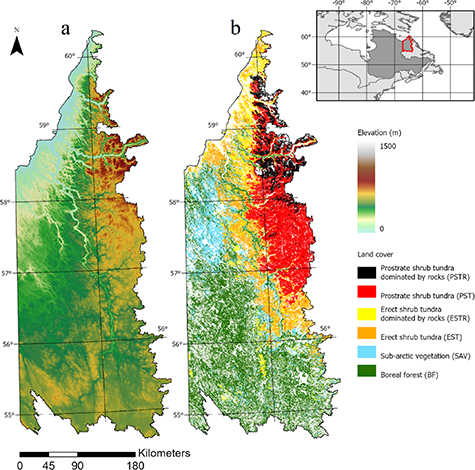
Figure 1. Location of the George and Koroc River basins in Northern Québec, Canada, showing (a) a physical map and (b) the main land cover as obtained from Leboeuf et al (2018), based on Landsat and RapidEye data (Leboeuf and Fournier 2015).
Download figure:
Standard image High-resolution image2.2. Landsat data and correction workflows
The study area covers 20 path/row numbers (tiles) of the Landsat Worldwide Reference System. We used all available standard Level-1 terrain-corrected orthorectified Landsat surface reflectance images from Collection 1 (geolocation error < 12 m) of the two month period from 1 July to 31 August for the 37 years from 1984 to 2019 (figure 1S (available online at stacks.iop.org/ERL/17/064051/mmedia)), archived by the Google Earth Engine (Gorelick et al 2017) platform as the image collection of United States Geological Survey Landsat 5/7/8 surface reflectance (SR). Images with an average cloud cover >80% were discarded as high cloud cover reduces the number of available ground control points and thus geolocation accuracy. Low-quality observations due to clouds, cloud shadows, cirrus, snow/ice, and scan-line corrector (SLC)-off gaps were identified using the Fmask approach (version 3.3) (Zhu and Woodcock 2012, Zhu et al 2015). Using ordinary least squares with the parameters from Roy et al (2016a), we converted OLI to ETM+. No correction was applied to TM or ETM+ as SR products from LEDAPS have been shown to be consistent through time, with no differences in the data from before and after the Landsat 7 ETM+ SLC failure in 2003, or between TM and ETM+ (Claverie et al 2015). Bidirectional reflectance distribution function (BRDF) effects were corrected using a c-factor approach (Roy et al 2016b) based on the RossThick-LiSparse BRDF model (Schaaf et al 2002) to account for the 'view angle effect', 'day of year effect', and the 'mean local time drift effect' (Gao et al 2014, Nagol et al 2015, Qiu et al 2021) which all add uncertainties to interannual comparisons of Landsat data (Zhang and Roy 2016, Roy et al 2020, Qiu et al 2021). Topographic correction was not considered necessary as the slope angles in the study area (quantile 90% = 7.75°) are too small to impact reflectance (Dymond and Shepherd 1999). The NDVI was computed using Normalized BRDF SR in the red and near-infrared spectral bands, retaining pixels with NDVI values >0.1 to assess trends in vegetated surfaces only (Fretwell et al 2011, Bayle et al 2021). The maximum NDVI (NDVImax) was computed as the annual maximum per pixel from the period 1 June–31 August of each year (Day of year ∼152–243). Due to variations in cloud cover, image density, and phenology NDVImax occurred on different dates each year. To prevent errors in NDVImax trend estimation, we discarded those years in which the date of NDVImax differed by more than ±2σ from the overall mean (figure 2S).
2.3. Climate data
Air temperatures and water conditions for our study area from 1984 to 2019 were obtained from the global monthly 4 km gridded TerraClimate data set available from the University Corporation for Atmospheric Research (Abatzoglou et al 2018) which combines high spatial resolution climatological normal from the WorldClim dataset with coarser, time-varying data from other sources to produce estimates of precipitation, water deficit, and temperature data, among others. From the monthly minimum and maximum temperatures, we computed the summer warmth index (SWI) as the sum of the mean monthly air temperatures exceeding 0 °C during the period from June to August, commonly used as an indicator of cumulative heat load in the Arctic (Bhatt et al 2017, Berner et al 2018, 2020). The sum of summer precipitation and the sum of summer water deficit as the respective sums of monthly precipitation and water deficit between June and August of each year.
2.4. Sampling design
Our study relies on two distinct samples of pixels both designed to minimize border effects and maximize within-pixel land cover homogeneity. Firstly, we selected pixels corresponding to each medoid of the six land cover classes using the tool 'Feature to Point' from ArcGIS 10.4.1 with 'Inside' option, which yielded 109 447 samples. To reduce spatial dependencies among samples, we removed samples where the nearest neighbour was closer than 300 m (leaving n = 86 339, figure 3S). We also discarded samples for which there were less than 20 years of Landsat records available (n = 85 830) and un-vegetated or sparsely vegetated pixels with a mean NDVI (1984–2019) lower than 0.1 to retain vegetated pixels only (n = 85 703). We did not account for human related land cover changes or fire which are both known to be extremely sporadic in our study area. Secondly, to understand the relation between NDVImax trends and climate, we calculated the spatial averages of the NDVI values obtained from the above approach for each 4 km pixel in the TerraClimate data set (n = 7933). Elevation and latitude were obtained from the 10 m spatial resolution regional hydro coherent digital elevation model by the Ministry of Energy and Natural Resources of Québec, and Natural Resources Canada (https://mern.gouv.qc.ca/repertoire-geographique/modeles-numeriques-terrain-hydro-coherents-echelle-regionale/), resampled at 30 m and extracted for the first sample set. Following the same procedure as for the NDVI data, we averaged this 30 m resolution elevation and latitude data to each 4 km TerraClimate pixel. Each TerraClimate pixel was assigned one class of land cover based on a majority rule from the first sample set.
3. Methods and statistical analysis
Temporal variability in NDVImax trends was assessed by fitting linear models to the period 1984–2019 using an 11 year rolling windows approach. This approach is similar to rolling averages, except that it uses a median-based linear regression rather than an average to each time period (window). NDVImax trends were computed for window widths ranging from 3 to 17 years and a rolling window width of 11 years was chosen as the best compromise between noise reduction and loss of relevant variability (figure 4S). This yielded 26 subsets for the median years 1989–2014. For example, the trend between 1991 and 2001 will be referred to by its median year and range: 1996 ± 5. We computed trends only for periods including at least ten years of available NDVImax. The linear model is based on the Theil-Sen single median slope and uses the 'mblm' R package (Komsta 2019). The Theil-Sen estimator of the linear trend is much less sensitive to outliers than a least squares estimator. We used the non-parametric, rank based, Mann-Kendall monotonic test to assess the significance of NDVImax time series trends. Direction, magnitude, and significance of NDVImax trends were analysed for the entire period and for each rolling window to assess the temporal variability.
For further analysis, we focused on the two periods that exhibited the strongest greening trends, henceforth referred as the two 'waves' W1 and W2. Significant (p < 0.05) greening trends for W1 and W2 were compared by computing simple Spearman correlations for each land cover type and all samples. Then, to compare both the directions and magnitudes of the W1 and W2 trends, we calculated an index  using atan2(W2/W1) in R based on standardized trends W1 and W2. The index was converted from radians to degrees which yielded angles between −180° and 180°, thus conserving the sign as opposed to the single-argument arctangent function which cannot distinguish between diametrically opposite directions. We then added 180° to α to change its range to 0°< α < 360°. This angular index allows us to combine the absolute magnitude of the greening trends and the relative difference in greening trend magnitude between W1 and W2 (figure 2). To investigate the spatial structure of the greening trends' temporal variability and to facilitate an easier interpretation, we binned
  into six equal-size bins (numbered 1–6 in figure 2) for each land cover type. We further investigated the relation between elevation and the six bins for the PSTR land cover type. We investigated the trends and inter-annual co-variation between SWI and significant greening trends (p < 0.05) for each rolling window and land cover type using our second sample set (n = 7933, 4 km resolution). Inter-annual co-variation was evaluated through the computation of NDVImax and SWI anomalies which were obtained as the residuals from linear model.

Figure 2. Interpretation of angles of the angular index  for comparing the two greening waves. Angles shaded in yellow correspond to more greening in W1 relative to W2, whereas angles shaded in blue correspond to more greening in W2 relative to W1. Darker colours correspond to more greening. Angles have been divided into six bins to facilitate easier comparisons (see text and figure 5).
Download figure:
Standard image High-resolution image4. Results
4.1. Spatiotemporal heterogeneity of greening
The emerging linear trend of NDVImax over the 36 year period indicates that over 90% of the pixels showed a significant increase in NDVImax (p < 0.05), particularly at latitudes between 57° and 59°N and below elevations of 500 m, which mostly corresponds to SAV and tundra dominated by erect shrub (EST and ESTR). Although greening occurred in all land cover types, BF and tundra dominated by prostrate shrubs (PST and PSTR) showed lower overall increases in NDVImax over time (figure 3). We found a strong temporal variability in both the direction and magnitude of NDVImax trends with two distinct waves of greening separated by a period with near-constant NDVImax values (figure 4). The first wave (W1) occurred between 1991 and 2001 (1996 ± 5) with almost 80% of sample points showing a significant greening (p < 0.05) which peaked at 0.016 NDVImax yr−1. The second wave (W2) occurred in 2011 ± 5 but was not as strong, with significant greening observed for only 30% of sample points at a lower average rate of 0.0075 NDVImax/year. In fact, at 83% of sample locations the greening was weaker in W2 compared to W1 (figure 5(b)), with only some higher elevation locations experiencing stronger greening during W2 (around 25% for PSTR) (figure 5(c)). There was no correlation between the greening rates measured in W1 and W2 at each sample point (Spearman's coefficient, ρ = 0.054) (figure 5(a)). Outside W1 and W2, only the PSTR land cover appears to display some greening (figure 5S). Interestingly, some pixels also displayed significant browning trends over the study period (figure 4(b)).

Figure 3. (a) Distribution of NDVImax trends (NDVImax yr−1) along latitudinal and elevational gradients. Ellipses represent 50% confidence intervals for each land cover type. (b) Distribution of NDVImax trends by land cover type. See figure 1 for abbreviations of land cover types.
Download figure:
Standard image High-resolution image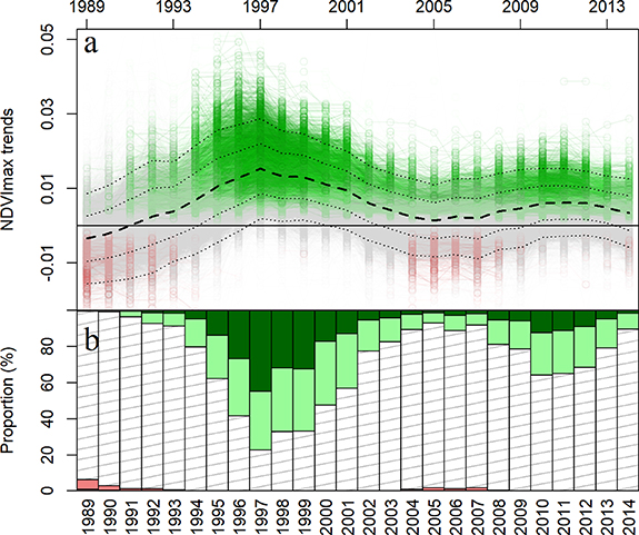
Figure 4. (a) Time series of NDVImax trends showing the mean slope in a median year as a thick, dashed line with standard deviations shown as thin dashed lines (SD and 2SD). Green lines and points represent significant and positive time series (p < 0.05), their red equivalents represent significant and negative time series (p < 0.05), and grey colour indicates a lack of statistical significance (p > 0.05). (b) Time series of the proportion of pixels with positive (dark green: p < 0.01; pale green: p < 0.05) and negative significant trends (dark red: p < 0.01; light coral: p < 0.05).
Download figure:
Standard image High-resolution image
Figure 5. (a) Comparing NDVImax trends for W1 (1996 ± 5) and W2 (2011 ± 5). The red line shows the linear model fit with correlation coefficient R2. The ellipses, from larger to smaller, represent the 25, 50, and 70% probability contours. The colours corresponds to α as defined in figure 2. (b) Percentage of pixels that fall into the six different bins of α (see figure 2) for each land cover type. (c) Distribution of land surface elevation for the different α bins of the PSTR land cover type. Refer to figure 1 for the abbreviations of land cover types.
Download figure:
Standard image High-resolution image4.2. Effect of summer warming on greening
Overall, summer precipitation did not exhibit significant trends over the 36 years although we did find some years with significant water deficits (1989, 1990, 2000, 2005 and 2012) (figure 6(a)). On average, high precipitation was observed during the 1990s and from 2006 to 2012. Time series of SWI showed significant warming during the 1990s marked by a strong negative anomaly in 1992, caused by the eruption of Mount Pinatubo (Lucht et al 2002). Since 2000, summer temperatures have varied and even decreased between 2005 and 2019, yet this period is marked by four of the warmest years since 1984 (2008, 2012, 2014, and 2019) (figure 6(b)). The two greening waves showed differing correlations with SWI (figure 7). While W1 was marked by a strong correlation between NDVImax and SWI (ρ = 0.57 ± 0.17), no significant correlation was found for W2 (ρ = −0.06 ± 0.25) (figure 7(a)). The same computation using NDVI and SWI anomalies showed similar results with moderate correlations for W1 (ρ = 0.3 ± 0.22) and no correlation for W2 (figure 7(b)). The distribution of correlations shows that almost all pixels exhibiting greening were correlated to summer warming in W1 (figure 7(c)). At the end of W1, a slight negative correlation between NDVImax and SWI anomalies was observed (figure 7(d)). These correlations were found for all land cover classes except arctic tundra (PST and PSTR). The positive correlation between NDVImax and SWI appears to last longer after W1 for PST and PSTR (figure 8(a)). Furthermore, we found stronger correlations between NDVImax and SWI anomalies for PSTR at the end of W1 (figure 8(b)).

Figure 6. (a) Time series of summer precipitation and summer water deficit from 1984 to 2019 based on the TerraClimate dataset. (b) Time series of Summer Warmth Index from 1984 to 2019. (c) Time series of Landsat-based NDVImax from 1984 to 2019. The dashed horizontal lines in each panel represent the averages while envelopes show one standard deviation.
Download figure:
Standard image High-resolution image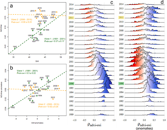
Figure 7. Correlation between (a) NDVImax and SWI, and (b) anomalies of NDVImax and SWI for W1 (green) and W2 (yellow). Spearman's correlation coefficients and corresponding standard deviation are shown for each wave. Distributions of Spearman's correlation coefficients for each rolling window for (c) NDVImax and SWI and (d) anomalies of NDVImax and of SWI. For (c) and (d), each year represents the median year of the rolling window.
Download figure:
Standard image High-resolution image
Figure 8. Distribution of Spearman's correlation coefficients for (a) NDVImax and SWI, and (b) anomalies of NDVImax and of SWI for each rolling window and land cover type. Time series were smoothed using LOESS regression. The coloured band represent the 97.5% confidence intervals for each land cover type. Refer to figure 1 for the abbreviations of land cover types.
Download figure:
Standard image High-resolution image
5. Discussion
Our detailed study of NDVI trends in northeastern Canada has provided significant insights to deepen our knowledge of the greening of Arctic and subarctic landscapes. First, while we showed that the study region experienced a strong greening trend over the 1984–2019 period, this trend is characterized by an important temporal heterogeneity as two distinct greening waves were observed during that period (figure 4). Second, all land cover types—i.e. from BF to arctic PST—displayed significant greening over that period although the two greening waves differed in intensity as greening was more intense in the first wave compared to the second one, but at different proportion depending on elevation (figure 5). Third, we found no consistent effect of summer warming on greening: while we observed strong relationship between NDVI and SWI during the first wave, there was no correlation during the second (figure 7).
Our study investigated the temporal heterogeneity of NDVI changes across a vast and diverse landscape. As our analysis relied on a unique high-resolution remote sensing approach for a wide range of vegetation types and topography, it inevitably calls into question the meaning of NDVI variations over time and the scale at which we observed it. In general, increases in NDVI can be attributed to changes in biomass production of established plants and/or to the establishment of newcomers with unknown consequences on NDVI values. Hence, an increase in NDVI of 0.1 over a particular time period but for two different vegetation types would not have the same ecological significance, illustrating the difficulty of using satellite-based proxies of vegetation cover to make statements regarding local ecosystems. In addition, the unavailability of in situ observation limits our ability to assign specific ecological processes to NDVImax trajectories (McManus et al 2012, Bonney et al 2018, Sulla-Menashe et al 2018). Thus, we rely on our reflectance correction workflow and the near absence of human impacts on our study area (section 2.2) to assume that significant changes in NDVI over time result from changes in vegetation cover at a pixel scale. Furthermore, by using high-resolution Landsat imagery, we minimize the probability of opposing trends occurring within a pixel as these small pixels represent more homogeneous vegetation types and topographies. This is key when studying vegetation dynamics across latitudes and altitudes as this necessarily involves complex ecotones and heterogeneous landscapes (Ropars and Boudreau 2012). Finally, our sampling strategy based on distance thresholding and land cover medoid selection, was designed to minimize these issues by limiting spatial autocorrelations. Overall, we are therefore confident that our approach is suitable to reliably identify real changes in ground vegetation.
Widespread greening has been reported in many cold, seasonally snow-covered ecosystems (Zhu et al 2016, Anderson et al 2020, Berner et al 2020, Choler et al 2021) as a response to the more pronounced warming they experienced over the last few decades compared to lower latitude and altitude ecosystems (Pepin et al 2015, Palazzi et al 2019). In fact, north-eastern Canada has been identified as a greening hotspot by Ju and Masek (2016) and Berner et al (2020) based on 1984–2012 Landsat time series data. Our results do corroborate their findings as more than 90% of our study region exhibited significant greening between 1984 and 2019. This homogenous greening in an area that harbours rather diverse vegetation zones and topographical gradients that generate strong environmental gradients over short distances is astounding, considering that greening occurred only on about 40% of the terrestrial land area in the Arctic (Berner et al 2020). Such results are likely related to the specific location of our study area, at the transition zone from forest/tundra to the Low Arctic, which is very responsive to warmer air temperatures (Epstein et al 2004, Walker et al 2006, Lantz et al 2010). In this particular region, as well as in other parts of Nunavik, the observed strong positive greening trend is believed to be closely associated to the expansion of Betula glandulosa Michx., the main 'species' involved in landscape-level shrubification (Ropars and Boudreau 2012, Tremblay et al 2012). Indeed, this species' radial growth has increased sharply in the 1990s (Ropars et al 2015) in response to warmer temperatures in this region (Bhiry et al 2011). The responsiveness of B. glandulosa to climate change could be due to a greater morphological plasticity, as shown for closely related species of the Betula genus (Shaver and Cutler 1979, Bret-Harte et al 2001).
We were able to demonstrate that the greening observed in our study region between 1984 and 2019 (figure 4) occurred in two distinct and relatively short greening waves lasting from 1991 to 2001 (W1) and 2006–2016 (W2). Historically, temporal patterns of NDVI variation have often been assessed by comparing two overlapping periods (Jeong et al 2012, Bhatt et al 2013, 2017, Berner et al 2020). Such studies found a systematic slowing in greening trends over the last 20 years in comparison to the 1990s. Similarly, since greening in W1 was stronger than in W2 this would also suggest a slowing of the observed greening trends (figure 5(a)), except at high altitudes where greening was stronger in W2 (figures 5(b) and (c)). Such a consistent pattern across most land covers suggests that plant communities respond to a common large-scale driver (figure 5S), likely warmer temperatures (figure 6(b)).
We explored the relation between NDVImax and summer temperature increase through two approaches. Our analysis showed a strong relation between NDVImax and SWI for W1 but not for W2, suggesting that large-scale changes in vegetation cover was triggered by warmer temperatures only in W1 (figures 7(a) and (c)). Comparatively, the analysis of inter-annual covariation (anomalies) between NDVImax and SWI revealed a moderate relation in W1 and no relation in W2 (figures 7(b) and (d)). The negative relation between anomalies of NDVImax and SWI toward the end of W1 corresponds to the inclusion of years characterized by extreme water deficit (2000 and 2005) in the 11 year rolling window, suggesting that drought stress could be the limiting factor that ended the first greening wave. The importance of drought on NDVI was indirectly proposed by Ropars et al (2015) based on growth ring data in western Nunavik. Indeed, they demonstrated that while B. glandulosa radial growth from 1986 to 2002 explained between 71% and 80% of the NDVI data variance, the reduced growth between 2000 and 2009 was likely due to negative water balance. In our study, the drought hypothesis is also consistent with the specific response of high-altitude land cover to summer warming (figure 8). As the evapotranspiration demand is likely lower for high-altitude ecosystems with a reduced vascular plant cover, years of drought should have a smaller impact on their primary productivity (Corona-Lozada et al 2019). In fact, land covers dominated by prostrated shrubs (PST and PSTR) tend to exhibit a more diffuse W1 than other low-altitude land cover types (figure 5S) which translates into a prolonged positive relation between NDVImax and SWI (figure 8(a)). Furthermore, there is a significant shift in time in the correlation between anomalies of NDVImax and SWI for PSTR despite the important water deficit observed throughout this period (figure 8(b)). For W2, no difference was found in the relationship between summer temperature and NDVImax among land covers. Interestingly, W2 was marked by three years of extreme temperatures (figure 6(b)) which did not result in water deficits as precipitations remained high (figure 6(a)). As heat waves accompanied by high precipitation are favourable to alpine vegetation growth (Corona-Lozada et al 2019), it is plausible that temperature remained the main driver of greening but through recurrent extreme heat events instead of long-term trends (Simpkins 2017). Another explanation could be that the second period of greening is the result of the warming observed in the 1990s, as temperatures remained stable between W1 and W2, but with a delay due to water balance deficits in the 2000s that prevented vegetation from fully benefiting from the initial warming. Finally, we did not analyse changes in herbivory pressure over time, though it has been shown that herbivores can alter tundra response to warming (Post and Forchhammer 2008, Campeau et al 2019). This might be of importance since the George River caribou herd (Rangifer tarandus L.) was abundant in our study region up to the 1990s, before declining progressively until the 2010s. These limitations should be considered for further research.
6. Conclusion
We demonstrated a strong temporal heterogeneity in the greening pattern along a large watershed in north-eastern Canada with two distinct greening waves (centred around 1996 and 2011) found during a 36 year period from 1984 to 2019. NDVI increased in all land cover types, from BF to arctic PST, strongly correlated with increased summer temperatures during the first wave but uncorrelated during the second one. We also showed that the first greening wave and its relation to summer warming lasted for a longer time in high-altitude vegetation. Our work explores a forsaken complexity of high latitude greening and has raised new questions that warrant further research highlighting the importance to include the temporal dimension. We emphasize that in order to disentangle the complexity of arctic greening, the temporal domain should be accounted for in conjunction with well-studied spatial gradients which result in the consideration of both forcings and ecological responses as non-stationary (Wolkovich et al 2014).
Acknowledgments
This research was developed in collaboration with the community of Kangiqsualujjuaq and supported by the Centre d'études Nordiques (CEN). Financial support was provided by OHMi-Nunavik—LabEx DRIIHM, French program 'Investissements d'Avenir' (ANR-11-LABX0010) managed by the French National Research Agency (ANR), Polar Knowledge Canada, ArcticNet (Network of Centres of Excellence of Canada), Crown-Indigenous Relations and Northern Affairs Canada (Indigenous Community-Based Climate Monitoring Program), NSERC-discovery grant (Lévesque). Authors acknowledge the support of the Community of Kangiqsualujjuaq to this project, especially for during the Imalirijiit field camp 2018 that facilitated access to field sites that stimulated the current analysis. Thank you to José Gérin-Lajoie, Xavier Dallaire and Geneviève Dubois for assistance in the field. We also thank Claude Morneau, Martin Simard, Hugues Dorion and José Gérin-Lajoie for support to different aspects of the project. Editorial assistance, in the form of language editing and correction, was provided by XpertScientific Editing and Consulting Services. Finally, anonymous evaluators contributed to improve the manuscript.
Data availability statement
The data that support the findings of this study are available upon reasonable request from the authors.