Warm Arctic−cold Siberia: comparing the recent and the early 20th-century Arctic warmings

Arctic sea ice extent has declined steadily by more than 10% per decade since the start of the satellite era (e.g. Stroeve et al 2011). While negative tendencies are observed for all seasons throughout the year, the most pronounced decline is observed in late summer and early autumn (Serreze et al 2007). Together with this sea ice decline, a strong near-surface Arctic warming has been recorded, especially during boreal wintertime (Screen and Simmonds 2010), attributed to the Arctic amplification of anthropogenic global warming (Serreze and Barry 2011). This amplification is characterized by Arctic temperature trends which are approximately twice as strong as the hemispheric trends (Semenov et al 2010).

This well-documented Arctic warming trend has been observed in conjunction with a winter cooling of the mid-latitudes in recent years, being particularly strong over central Siberia (Cohen et al 2014, Vihma 2014, Shepherd 2016, Overland et al 2016 and references therein). Patterns of intensified cold spells and extreme snowfall events were also documented over the other Northern Hemisphere mid-latitude regions (Cohen et al 2007, Ghatak et al 2012, Vihma 2014, Wegmann et al 2015, Orsolini et al 2016). The Eurasian variant of this phenomenon has been termed 'warm Arctic–cold Siberia,' or WACS—similar definitions such as 'warm Arctic–cold Eurasia' are essentially describing the same pattern (Petoukhov et al 2013)—since the appearance of a cold anomaly over Siberia was found in conjunction with warming over the Barents–Kara Sea (BKS) region (Overland et al 2011, Inoue et al 2012).

Several studies investigated the possible mechanisms behind this counterintuitive process. Honda et al (2009) first demonstrated that the WACS pattern can be attributed to sea ice loss over the BKS, which in turn triggers increased turbulent heat fluxes from the ocean to the atmosphere. It was found that an increasing autumn surface heat flux from the open waters to the cooler atmosphere with anomalous warming of the lower atmosphere triggers increased baroclinic wave activity and higher amplitudes of Rossby waves, which favor the development of blockings and extreme weather such as cold air outbreaks (Francis et al 2009, Honda et al 2009, Orsolini et al 2012, Cohen et al 2014, Mori et al 2014, Jaiser et al 2016, Nakamura et al 2016, Luo et al 2016, Sorokina et al 2016). Understanding the causes of such extreme events is therefore of large societal importance (Overland et al 2016, Francis 2017).

There remains uncertainty about whether the winter WACS pattern is a delayed response to decreased autumn sea ice (Honda et al 2009, Overland et al 2011, Wegmann et al 2015, Suo et al 2016, Wu 2017) via a stratospheric feedback (Jaiser et al 2012, Cohen et al 2014, García-Serrano et al 2015, Jaiser et al 2016, Ruggieri et al 2017, Kretschmer et al 2017) or if it is an immediate response triggered by winter sea ice anomalies (Hori et al 2011, Inoue et al 2012, Sorokina et al 2016, King et al 2016). The physical feedbacks, as summarized by Cohen et al (2014), are thought to induce a causal chain process, where reduced autumn sea ice warms the lower troposphere, which increases geopotential heights, shifts stormtracks and increases Eurasian snow cover in October and November. This setting favors high Rossby wave numbers, with vertical propagation of Rossby wave energy, resulting in a weakening polar vortex and a stratospheric warming event (Gastineau et al 2017). Subsequently, tropospheric circulation anomalies appear with a few weeks' lag.

Despite the uncertainty of the temporal relationship, the BKS region emerges as the core region for atmospheric feedbacks triggering the WACS (Inoue et al 2012, Outten et al 2013, Luo et al 2016, Zhang et al 2016, Screen 2017). Reduction in BKS sea ice can be caused by several mechanisms, including warm Atlantic water inflow (Miles et al 2014, Nakanowatari et al 2014, Årthun et al 2017), atmospheric heat advection (Zhang and Li 2017) or atmospheric radiation feedbacks (Park et al 2015).

Recent studies based on sensitivity experiments with atmospheric global climate models (AGCMs) nevertheless question the proposed link between sea ice reduction and the WACS pattern (Sato et al 2014, Sun et al 2016, McCusker et al 2016, Boland et al 2017, Collow et al 2016). On the other hand, some model studies (Honda et al 2009, Nakamura et al 2015, Kretschmer et al 2017, Pedersen et al 2016, Crasemann et al 2017, Ruggieri et al 2017) did indeed show realistic tropospheric sensitivity to sea ice forcing. Cohen et al 2012 as well as Cohen 2016 pointed out that many of the current generation of AGCMs may lack the ability to simulate the influence of Arctic amplification on mid-latitude climate. This raises the question of whether the WACS pattern can result from the random sampling of climate states undergoing chaotic nonlinear variability, or rather is being controlled by the proposed causal link to sea ice, but with this physical mechanism missed in the state-of-the-art AGCMs (Francis 2017).

Here we utilize long-term reanalyses and reconstruction datasets to investigate the 'early twentieth-century Arctic warming' (ETCAW) which reached its peak warming at the beginning of the 1940s but started around 1910. Compared to the present Arctic warming, the ETCAW was mainly confined to the European Atlantic sector (Scherhag 1939, Bengtsson et al 2004, Wood and Overland 2010, Bekryaev et al 2010). In the vertical, recent maximums of temperature anomalies are mostly found at the surface whereas the maximum warming of the ETCAW was located in the mid troposphere (Grant et al 2009, Brönnimann et al 2012). Possible warming mechanisms include warm air advection by southerly winds (Wood and Overland 2010, Wegmann et al 2017) as well as increased winter sea-surface temperatures (SSTs) (Johannessen et al 2004, Bengtsson et al 2004, Semenov and Latif 2012). Analyzing 26 simulated Arctic warming events, Beitsch et al (2014) found a triggering warming ocean signal that induces atmospheric changes, including increased stationary eddy heat transport into the Arctic domain. Recently, Tokinaga et al (2017) were able to reproduce the large-scale ETCAW by introducing historical SST forcing in an atmosphere–ocean coupled global climate models (AOGCM), underlining the importance of SSTs in the onset and evolution of the ETCAW.

Paleoclimatic data suggest that, until the beginning of the twenty-first century, the ETCAW was unique in magnitude and rate for at least the last 1500 years in the Arctic domain (Kaufman et al 2009, Pages 2 K Consortium 2013, Opel et al 2013). Therefore, the ETCAW offers a unique opportunity to investigate feedbacks of global climate during Arctic warming periods.

The goal of this study is to demonstrate the consistency between both periods, of the sea ice decline, the covariability of the sea ice with atmospheric temperature and heat fluxes, and their impact on the Arctic region. For this purpose, we compare decadal temperature trend patterns among the two warming events (ETCAW and present) and the dynamical conditions leading to the associated WACS pattern. We focus on the boreal winter (DJF) temperatures and their relationship with September sea ice extent in the BKS region using regression analysis for quantifying the role of different mechanisms.

The paper is organized as follows: section 2 describes the data and methods used. In section 3 we introduce the ETCAW and the respective WACS patterns, whereas section 4 investigates the dynamical process behind that pattern. These results are discussed in section 5 and finally summarized in section 6.

2.1. Atmospheric reanalyses

2.2. Reconstruction data

2.3. Global climate model

2.4. Sea ice data

For recent sea ice data we use the ERA-Interim sea ice concentration (SIC), which is highly correlated to the NSIDC sea ice data. For instance, Sorokina et al (2016) reported no differences between these two datasets.

For the ETCAW period we investigate five different SIC datasets, namely the three products used in the long-term reanalyses (see table 1) as well as the independent sea ice concentration data by Walsh et al (2017) plus the sea ice output from the centennial ocean reanalysis ORA-20C by the ECMWF (De Boisséson et al 2017). Although there are considerable uncertainties regarding the Arctic sea ice conditions before 1950, Connolly et al (2017) recently provided a new reconstruction of historical Arctic sea ice which supported the melting period between 1910–1940. Moreover, Alekseev et al (2016) found a substantial decrease of September Arctic sea ice between 1930–1940 in their assessment of Arctic sea ice in the 20th century. Thus, besides the reconstructions used in this study, other independent datasets suggest a sea ice reduction during the ETCAW period.

We define the BKS as region bounded by 30–90° E, 65–85° N and focus on September sea ice. In September, sea ice reaches its annual minimum and open-water regions provide a strong heat and moisture release to the cold Arctic atmosphere (Jaiser et al 2016). We checked using different autumn months between September and December and found that regression with September sea ice best represents the DJF temperature trend, especially so for the ETCAW (see supplementary figure 1 available at stacks.iop.org/ERL/13/025009/mmedia). However, we did not find a large difference among all autumn months. All sea ice time series are normalized with respect to their time periods (1987–2016 for the current warming and 1911–1940 for the ETCAW). Luo et al (2016) found no notable difference between using original and de-trended sea ice time series in their feedback study (which we confirmed in supplementary figure 2), therefore we use original time series from here on. This highlights the fact that interannual variability is a key factor for investigating feedbacks rather than the overall trend. Figure 1 shows the normalized BKS sea ice concentration time series for all reconstructions, including both warming periods (for un-normalized BKS sea ice time series see supplementary figure 3). As can be seen, differences in reconstructions for the ETCAW can reach up to one standard deviation. However, when taken as average, the ETCAW BKS sea ice evolution is very similar to the recent BKS sea ice decrease. Therefore, it seems reasonable to use the ETCAW as an analogue (in terms of BKS sea ice impacts) to the recent Arctic warming (RAW) period.

Zoom In Zoom Out Reset image size

Zoom In Zoom Out Reset image size

2.5. Regression on SIC

We use the above-mentioned normalized BKS SIC time series to investigate linear relationships between atmospheric variables and the sea ice evolution. For this purpose, we project the respective anomaly fields onto the SIC time series for the ETCAW period 1911–1940 and the RAW period 1987–2016. For the main manuscript it will be the normalized HadISST2 BKS SIC time series for the ETCAW and the normalized ERA-Interim BKS SIC time series for the RAW. To test the regression coefficient against the null hypothesis, we use a two-sided Student's t-test, which is also used for inferring the significance of the trends. For enhanced readability, the regressed fields are multiplied by −1 to correspond to a signal resulting from reduced sea ice.

Zoom In Zoom Out Reset image size

3.1. Eurasian temperature patterns during Arctic warmings

3.2. Tropospheric dynamics associated with sea ice loss

To investigate the tropospheric dynamics associated with the WACS pattern, figures 5(a)−(d) shows 500 hPa geopotential anomalies regressed onto the same BKS SIC time series that were used in previous figures. For the RAW, a strong positive anomaly dominates the Arctic, extending southward over western Russia and reaching the Caspian Sea. This high-pressure anomaly is flanked by two low-pressure systems leading to a zonal-to-meridional transition of the heat advection. For the ETCAW in ERA20C, a similar structure can be observed for Eurasia. Using the Walsh et al (2017) or ORA20C dataset, this transition becomes even more apparent (see supplementary figure 6).

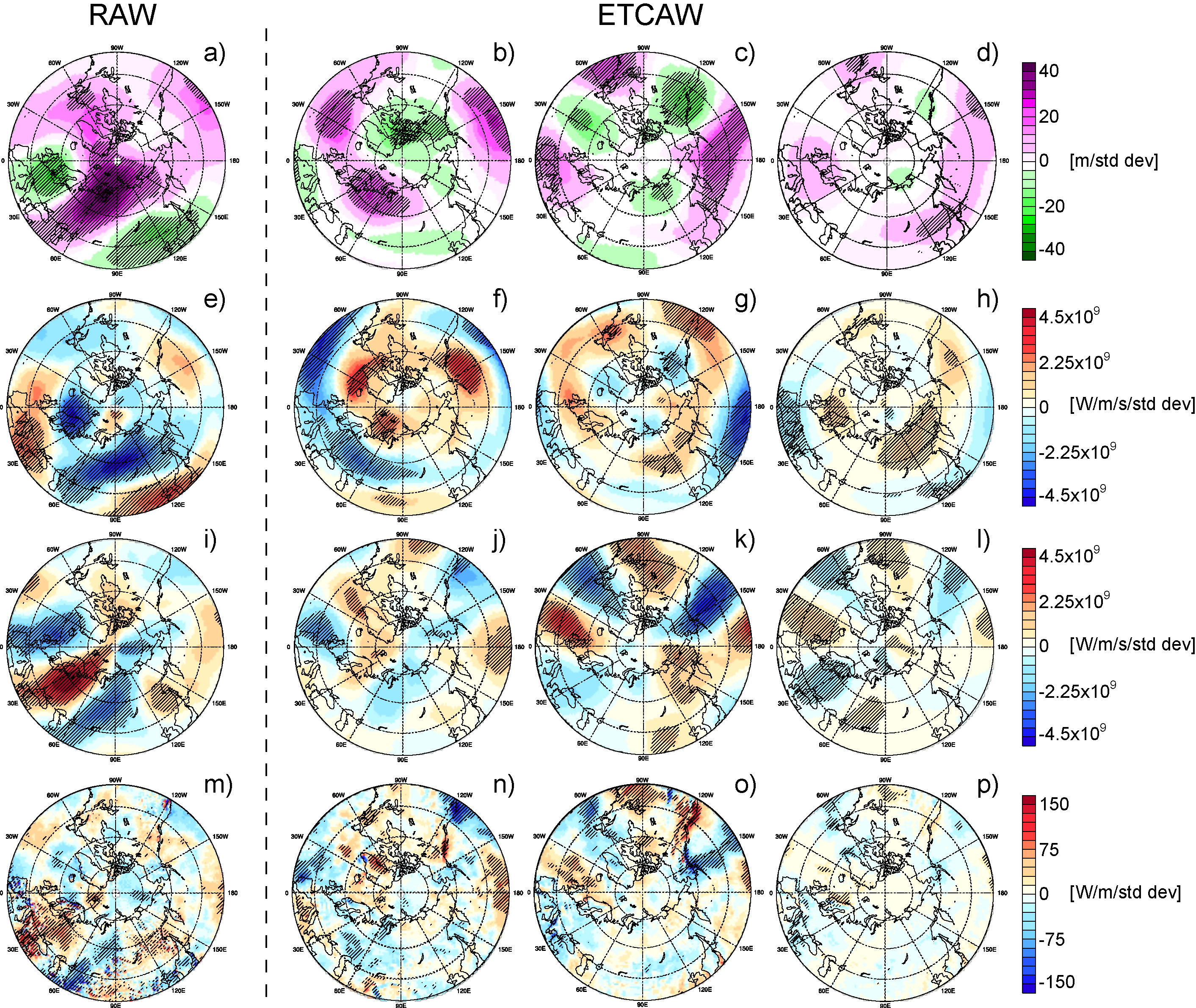
The geopotential height patterns shown figures 4(a)−(d) cause anomalous heat advection over the Eurasian domain. We regressed horizontal heat-flux anomalies onto the BKS SIC time series to investigate the response of atmospheric heat transport to the SIC signals during ETCAW and RAW (figures 4(e)−(p)). For the RAW, a wave train-like structure in meridional heat flux (figures 4(i)-(l)) over Europe and Eurasia is clearly visible as well as the westward heat flux over northern Europe and Siberia. This means that cold air is transported southward from the Arctic into large parts of eastern Siberia. Moreover, the westward pattern over the mid-latitudes combined with the strong waviness reduces heat advection by westerlies, which usually advect warm, maritime air masses. For the ETCAW, ERA20C shows eastward heat flux over large parts of the Central Arctic with Atlantic air masses being advected to Northern Russia. Meridional heat-flux patterns in ERA20C are homologous to the trend pattern as well, with southward fluxes from the Arctic towards Central Siberia. We note, that the wave train-like pattern in meridional heat flux derived by regressing heat fluxes onto HadISST2.0 SIC over Eurasia does not hold statistical significance. However, using the Walsh et al (2017) or the ORA20C sea ice reconstruction together with ERA20C atmospheric fields, the southward cold-air transport becomes significant and the transport pattern largely resembles the RAW pattern (see supplementary figure 7). As for the RAW, the westward circulation over large parts of the Eurasian mid-latitudes reduces the advection of maritime air masses, supporting the cooling by the Arctic air masses coming from the north.

Zoom In Zoom Out Reset image size

Zoom In Zoom Out Reset image size

For the ERA20CM selected 'best guess' member, regression patterns are different from the ERA20C. The regression pattern shows no significant mid-latitude heat advection reduction but instead widespread eastward heat-flux increase in response to the SIC evolution, similar to the ERA20CM ensemble mean. This similarity is even more striking in the case of Arctic to mid-latitude heat transport, where the wave train-like structure over Eurasia shows the opposite sign to the heat transport in ERA20C.

Based on the comparison between the trend and regression patterns, we find that the overall winter temperature and heat-flux trend is largely congruent to a reduction of September BKS sea ice. Both eastward zonal flux and meridional flux culminate in integrated heat flux convergence (figures 4(m)−(p)), which shows a clear negative signal over Central Siberia for the ETCAW, and a little bit further to the east in the case of the RAW. Since ERA20CM already failed to reproduce the horizontal heat fluxes, no such areas of negative heat convergence can be found in the model fields.

In general, the structure of geopotential height anomalies in ERA20C is visible in neither the ERA20CM selected best guess member, nor the ensemble mean. Thus, the resulting heat-flux advection in ERA20CM is unlike what the reanalyses show. Moreover, this indicates that the influence of the sea ice on the models is not strong enough to reach the mid- and upper troposphere in the same way as is proposed in reanalyses.

Differences between reanalyses and the AGCM become even more striking when looking at the zonal mean temperature response to BKS SIC evolution throughout the troposphere over northern Eurasia (figure 5). Comparing the RAW (figure 5(a)) and ETCAW (figure 5(b)) temperature distribution reveals the strong gradient between the Arctic and the mid-latitude. The Arctic experiences a strong warming deep into the troposphere whereas south of 60°N the signal turns to a cooling that dominates the whole troposphere for the RAW and up to 300 hPa for the ETCAW. Note that the surface cooling is not significant for ERA-Interim, which is probably based on the chosen domain for the zonal average (10–180° E, 30–90° N) since eastern Europe shows a warming response for the RAW. Again, the mid-latitude cooling response in ERA20C can be strengthened by using different sea ice reconstructions. However, the structure of the WACS stays the same, regardless of the sea ice reconstruction or the reanalysis at hand (supplementary figure 8). Zonal mean plots of geopotential heights (figures 5(e)−(f)) show nicely the elevated geopotential height (GPH) values over and the Arctic in periods of Arctic warming. Differences between the RAW and ETCAW appear in the northern most gridboxes, where the ETCAW shows slightly reduced GPH values in the lower troposphere. As a consequence of the GPH negative gradient between the Arctic and the mid-latitudes, a strongly reduced zonal wind appears throughout the troposphere in both Arctic warming cases, reaching from roughly 40°–60° N. These reduced zonal winds are connected to the reduced eastern heat flux shown in figures 4(e)−(h).

On the other hand, both the ERA20CM best guess member (figure 4(c)) and the ensemble mean (figure 4(d)) show no mid-latitude cooling in response to the BKS SIC. Instead widespread tropospheric warming can be found in the mid-latitudes. The ERA20CM best guess member even fails to reproduce the widespread tropospheric warming response over the Arctic. Moreover, both ERA20CM analysis fields show nearly mirrored zonal mean zonal wind fields (figures 5(k)−(l)) compared to the reanalyses. Increased zonal wind dominates the mid-latitudes between 40°–60° N, which is a result of shifted geopotential height locations.

We used a variety of gridded atmospheric datasets: AGCM simulations, reanalyses and reconstructions, to address some of the open questions regarding the cause and manifestation of the WACS surface temperature pattern—one of the most remarkable counterintuitive features associated with Arctic amplification.

A key question in the ongoing discussion about the origin of WACS pattern is whether the observed temperature pattern is caused by a chain of physical processes (Honda et al 2009, Overland et al 2011, Cohen et al 2014, García-Serrano et al 2015, Jaiser et al 2016), or if it is part of internal variability and its occurrence results from the random sampling as revealed by the model sensitivity studies (Sun et al 2016, McCusker et al 2016, Boland et al 2017, Collow et al 2016).

We try to address this question by comparing the two Arctic warming periods (ETCAW and RAW), both characterized by decreasing BKS SIC using different reanalyses and comparing them with AGCM simulations. Using a re-analysis (ERA20C) and a model simulation (ERA20CM) using the same ECMWF atmospheric model allows us to directly infer the impact of assimilated data, since all boundary conditions are the same for both datasets.

Our results support some of the aforementioned findings concerning the RAW: Striking similarities are found between the ETCAW and RAW periods, namely the manifestation of the WACS pattern and its dynamical background, the reduced atmospheric heat transport to central Eurasia. Our study suggests that the changes in the autumn SIC in the BKS largely explain the observed temperature trends by modulating the pressure patterns in the upper troposphere, which consequently impact the heat-flux convergence over the mid-latitudes (Cohen et al 2014, Francis and Vavrus 2015). In this case, September sea ice concentration affects the surface turbulent heat fluxes over the BKS in the following autumn months (supplementary figure 9). Reduction in BKS sea ice can be caused by several mechanisms such as a general rise in north Atlantic SSTs (Miles et al 2014, Nakanowatari et al 2014, Årthun et al 2017), atmospheric heat advection (Zhang and Li 2017) or increased longwave radiation (Park et al 2015). Future studies are needed to address the ultimate cause behind the sea ice decrease in the ETCAW. However, we found that detrended September BKS SIC explains the zonal mean trend over Eurasia for the ETCAW better than a detrended September or DJF AMO index (supplemetary figure 10).

The main reason for the reduced heat convergence seems to be a positive geopotential height anomaly in the upper troposphere located over the BKS region, which is in agreement with recent studies concerning the RAW (Honda et al 2009, Petoukhov and Semenov 2010, Kim et al 2014, Kug et al 2015, Luo et al 2016). Our results disagree with the findings of Sorokina et al (2016), who found that BKS sea ice reduction and the following turbulent heat flux over the ice-free areas is not enough to explain the WACS pattern. However, we want to underline the findings of Gastineau et al (2017), stating that the co-variability of sea ice, Eurasian snow and hemispheric SSTs is important for the generation of the WACS pattern. Further research is needed to address this coupled ocean–cryosphere–atmosphere pattern, which is still a challenge for recent models.

Our findings are qualitatively independent of the sea ice reconstruction at hand and it is mainly the significance of the resulting patterns that is impacted by the choice of SIC reconstruction. Interestingly, using the Walsh et al (2017) dataset for the ETCAW period resulted in the highest confidence for the regression analysis. Moreover, the respective ETCAW 500 hPa GPH and heat flux anomalies show a very high similarity with those obtained for the RAW period, although the sea ice reduction trend between 1911–1940 in the Walsh et al (2017) dataset is the weakest among the investigated SIC reconstructions.

Furthermore, our results support recent studies (Cohen 2016, Francis 2017, Gastineau et al 2017) which argue that current AGCMs lack the capability to properly reproduce climate feedbacks triggered by the Arctic sea ice decline. Although we found 1 out of 10 ensemble members which reproduced the WACS pattern relatively well for the analysis of trends, the regression analysis showed no connection to the underlying dynamics and disagreed with the findings from ERA20C. Additionally, the ERA20CM ensemble mean failed to reproduce the observed temperature and circulation fields for the ETCAW. Reasons for the flaws in the AGCM models can be manifold. Francis (2017) points out that boundary layer processes, troposphere–stratosphere coupling and high sensitivity to tropical climate are issues in modelling an appropriate Arctic amplification and sea ice loss response. In fact, model experiments in Tokinaga et al (2017) show that the correct WACS temperature pattern response is found if the model is forced mainly with tropical SST variability rather than mid-latitude SST variability. We found similar results for the ERA20CM ensemble (see supplement figure 11), underlining the points made by Cohen (2016). Smith et al (2017) show that modeled response to Arctic sea ice loss depends on the background state of the model and pointed out differences between AOGCMs and AGCMs response. They further noted that the response is sensitive to the detailed properties of planetary wave propagation into the stratosphere. Moreover, different factors of natural variability may play a role in the formation of the WACS pattern, which are not captured in AGCMs. Further studies are needed to investigate the disagreement between (some) GCM experiments and observed responses.

Several simulated and reconstructed gridded datasets were used to examine the link between September SIC in the BKS, atmospheric conditions and the WACS temperature pattern in winter. We found evidence for a manifestation of this temperature pattern not only during the current ongoing Arctic warming period (RAW), but also for the Arctic warming between 1910–1940 (ETCAW). Regression analysis with normalized SIC from the BKS region indicates that the overall temperature and heat-flux trend is largely congruent to a reduction of September BKS sea ice.

Upper troposphere conditions point towards a strengthened atmospheric blocking over the BKS, implying the advection of cold air from the polar regions to central Siberia on its eastern flank. Moreover, this blocking triggers a more meridional circulation, reducing the strength of the warm air advection by the westerlies. Comparison of the long-term climate reanalysis ERA20C with its parent model run (ERA20CM) forced by the same sea ice and SST boundary conditions suggests that this particular AGCM lacks the ability to reproduce the atmospheric conditions following low-sea ice years, both at the surface and in the upper troposphere.

These findings are consistent with several recent studies and provide the foundation for analyzing the validity of the recent theories proposing a link between reduced SIC in the BKS and the WACS. To identify the specific deficiencies in AGCMs remains an open task. Moreover, since only one AGCM was used in this study, a variety of AGCM ensemble runs are needed to clearly rule out the possibility of the occurrence of WACS pattern due to random sampling. However, future projections and impact studies of Arctic warming periods should take into account a possible deficit in the large-scale response of sea ice on the mid-latitudes in models. Upcoming high-resolution reanalyses and reconstructions will improve the understanding of the WACS during the early twentieth century and offer further insights into a possible surface–stratosphere connection triggered by sea ice reduction, snow-cover changes and decadal SST changes.

We thank the ECMWF (Reading, UK) for making available the ERA-Interim, ERA-20C and CERA-20C reanalyses as well as ESRL NOAA (Boulder, USA) for the provision of the 20CR reanalyses. This work was supported by the BELMONT Fund ARCTIC-ERA project funded by the Agence Nationale de la Recherche (Paris, France) and by the EU-funded FRAGERUS-MRCM project. OZ was also supported by the Russian Ministry of Education and Science under Agreement # 14.616.21.0035 (identification no. RFMEFI61615X0035). YOR is supported by the Research Council of Norway (Grant SNOWGLACE #244166). The Authors are thankful to Eric de Boisséson for providing ORA20C SIC data, to Stefan Brönnimann for insightful comments and to Morgan Gray for editorial support.