Climate Change-Induced Emergence of Novel Biogeochemical Provinces
 Gabriel Reygondeau1,2*
  William W. L. Cheung1
  Colette C. C. Wabnitz1,3
  Vicky W. Y. Lam1
  Thomas Frölicher4,5
  Olivier Maury6
- 1Institute for the Oceans and Fisheries, The University of British Columbia, Vancouver, BC, Canada
- 2Department of Ecology and Evolutionary Biology, Max Planck – Yale Center for Biodiversity Movement and Global Change, Yale University, New Haven, CT, United States
- 3Stanford Center for Ocean Solutions, Stanford University, Stanford, CA, United States
- 4Climate and Environmental Physics, Physics Institute, University of Bern, Bern, Switzerland
- 5Oeschger Centre for Climate Change Research, University of Bern, Bern, Switzerland
- 6Marine Biodiversity, Exploitation and Conservation, Institut de Recherche pour le Développement, Ifremer, Université de Montpellier, CNRS, Sète, France
The global ocean is commonly partitioned into 4 biomes subdivided into 56 biogeochemical provinces (BGCPs) following the accepted division proposed by Longhurst in 1998. Each province corresponds to a unique regional environment that shapes biodiversity and constrains ecosystem structure and functions. Biogeochemical provinces are dynamic entities that change their spatial extent and position with climate and are expected to be perturbated in the near future by global climate change. Here, we characterize the changes in spatial distribution of BGCPs from 1950 to 2100 using three earth system models under two representative concentration pathways (RCP 2.6 and 8.5). We project a reorganization of the current distribution of BGCPs driven mostly by a poleward shift in their distribution (18.4 km in average per decade). Projection of the future distribution of BGCPs also revealed the emergence of new climate that has no analog with past and current environmental conditions. These novel environmental conditions, here named No-Analog BGCPs State (NABS), will expand from 2040 to 2100 at a rate of 4.3 Mkm2 per decade (1.2% of the global ocean). We subsequently quantified the potential number of marine species and annual volume of fisheries catches that would experience such novel environmental conditions to roughly evaluate the impact of NABS on ecosystem services.
Introduction
The biosphere is partitioned according to well-defined biomes corresponding to unique sets of physical, chemical and biological conditions. On land, biomes such as “desert,” “mountain,” or “forest” can be delineated by environmental variables such as temperature, precipitation and altitude (Peel et al., 2007; Sayre, 2014). Similarly, the ocean has been subdivided in various ways, using either expert opinion or data driven methods based on both biotic and abiotic components of the marine realm (Kavanagh et al., 2004; Oliver and Irwin, 2008; Reygondeau and Dunn, 2018). The widely accepted system of ocean provinces elaborated originally by Longhurst (2007) covers both open ocean and coastal zones. Two levels structure Longhurst’s province system. The first one distinguishes coastal and open ocean areas and subdivides them into temperate, tropical and polar biomes. The second sub-divides each of the coastal and oceanic biomes into oceanographically, ecologically and topographically homogeneous regions. This results in 56 distinct biogeochemical provinces (BGCPs) that have been shown to be closely related to global patterns in marine biodiversity (Pauly, 1999; Beaugrand et al., 2000), ecosystem functions and services such as fisheries productivity (Chassot et al., 2011; Demarcq et al., 2012; Reygondeau et al., 2012).
While the relevance of Longhurst’s BGCPs to partition the ocean into homogeneous environmental and ecological regions has been established (Reygondeau et al., 2012), their delineation has been modified to improve their representativeness of the biogeography of diverse biological communities (Reygondeau et al., 2013). Specifically, Reygondeau et al. (2013) have shown how seasonal and inter-annual climate variability – such as such as such as El Niño Southern Oscillation (ENSO) event– modifies BGCPs’ boundaries and drives their reorganization.
Climate change is expected to lead to drastic changes in ocean conditions. Oceans have already absorbed more than 93% of the heat resulting from the accumulation of greenhouse gases. They are rapidly getting warmer, less oxygenated (Gattuso et al., 2015) and changes in the seasonality of oceanographic conditions have already been reported. These oceanographic changes will alter the delineation and location of the BGCPs. Notably, some variables are expected to reach levels that are beyond those observed in recorded history (Froelicher et al., 2016). As a result, existing BGCPs might not be able to characterize regions where changes are projected to exceed the range of past observations. Such “novel” climatic zones have already been identified in the terrestrial realm. They have also been reported during marine heatwaves (Frölicher et al., 2018; Oliver et al., 2018).
In this study, we test the hypothesis that climate change might result in a large-scale bio-geographic re-organization of the oceans accompanied by the emergence of novel BGCPs. In particular, we examine the extent to which these novel BGCPs might overlap with marine biodiversity and fisheries (Cheung et al., 2016b; Cheung, 2018). For this purpose, we use the numerical approach described in Reygondeau et al. (2013) to analyze projected ocean conditions from three Earth System Models (ESM; Institut Pierre Simon Laplace, Max plank Institute and Geophysical Fluid Dynamics Laboratory models) under two climate change scenarios (the “strong mitigation” Representative Concentration Pathway, or RCP 2.6, and “business-as-usual” RCP 8.5). For each ESM and RCP scenario we calculate the projected annual average distribution of each BGCP from 1950 to 2100. We then identify regions that are characterized by novel combinations and levels of oceanographic variables and that have therefore never been observed historically. We name these novel BGCPs No Analog Biogeographical State regions (NABS). We quantify the timing of NABS emergence and evaluate the potential consequences on marine biodiversity and key marine ecosystem services.
Materials and Methods
Environmental Data
The ocean properties that we used to delineate the BGCPs from 1950 to 2100 were based on outputs from three ESMs. They include annual average surface (average between 0 and 10 m)and bottom sea water temperature (°C), oxygen concentration (ml.L–1), salinity, pH, surface net primary production (mgC.km2.year–1),particulate organic carbon concentration (mgC.km2.year–1) and sea ice coverage (%). These data have been simulated by the Geophysical Fluid Dynamics Laboratory Earth System Model (GFDL ESM2M), the Institut Pierre Simon Laplace Climate Model (IPSL-CM5-MR) and the Max Planck Institute for Meteorology Earth System Model (MPI-ESM). They were made available through the Coupled Model Intercomparison Project phase 5 (CMIP5; Taylor et al., 2012). The ESM outputs were re-gridded onto a regular grid of 0.5° of latitude by 0.5° of longitude using the nearest neighbor method and values in coastal cells were extrapolated using bilinear extrapolation. In addition, annual climatologies of euphotic depth (Morel et al., 2007), mixed layer depth (de Boyer Montégut et al., 2004), and bathymetry (Smith and Sandwell, 1997) were also used to delineate BGCP boundaries. These variables were gathered from observations and are here used to optimize the quantification of the environmental envelopes of specific BGCPs such as frontal oceanic systems, coastal regions or boundary of oceanic subtropical gyres.
The ESM outputs for the future period (2006–2100) were simulated under RCP 2.6 and RCP 8.5. The RCP 2.6 is a lower emission “strong mitigation” scenario under which the radiative forcing trajectory peaks at 3 W.m–2 before 2100 and then is followed by a decline to 2.6 W.m–2 by 2100. The RCP8.5 is a high emission “business-as-usual” scenario with a rising radiative forcing pathway leading to 8.5 W.m–2 by 2100.
Modeling the Geography of BGCPs
To delineate the BGCPs’ boundaries for each year from 1950 to 2100, we applied the numerical approach described in detail in Reygondeau et al. (2013). The approach quantifies the environmental envelopes of each BGCP based on the variables described above and projecting their future spatial distribution (Figure 1). First, the spatial coordinates of the boundaries for each BGCP as defined by Longhurst (2007) were retrieved (Figure 1A). Second, to include the monthly variation of each variable and characterize the discrete set of environmental conditions that characterize each BGCP, we obtained monthly values of the ESM outputs for each variable and spatial cell in each BGCP for the time period January 1970 to December 2000. This time period represents the timeframe over which the BGCP delineation was defined originally. We here used all environmental variables (surface and bottom) for BGCP located in the coastal biome and only surface environmental variables for BGCP located in the tropical, temperate and polar biomes (see Supplementary Table 1). We obtained 56 matrices of environmental properties (one for each province) named Xn1,p,z (n1 = 360 months, p = x environmental variables, z = number of geographical cells of the selected province). Third, we quantified the environmental envelope of each BGCP using three environmental niche models (ENM): Non-Parametric Probabilistic environmental niche model (Beaugrand et al., 2011), Maxent (Phillips et al., 2004), and boosted Regression Trees (Elith et al., 2008). We treated spatial cells included in each distinct BGCPs as a set of “occurrence records” analogous to species distributions and applied each ENM to model the environmental envelopes of each BGCP. We applied a multi-model ensemble approach to capture the uncertainty associated with the different numerical methods. Finally, we computed the time-dependent spatial distributions of the probability of occurrence (values ranging between 0 and 1) of each BGCP from the annual average ENM outputs for each ESM and each RCP scenario. Global BGCP division is then identified by attributing the geographical cell to the BGCP with the highest probability of occurrence for each year in each geographical cell and year.
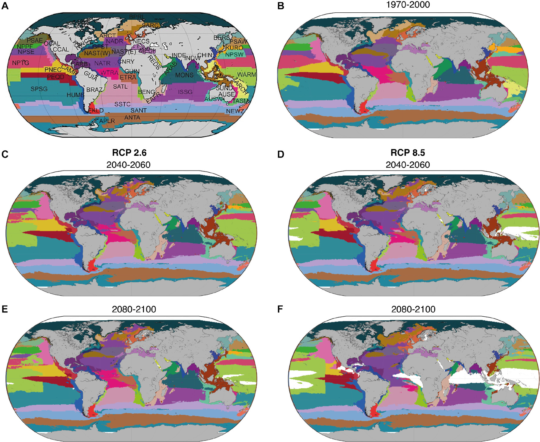
Figure 1. Distribution of the 56 BGCPs: (A) according to Longhurst (2007); and for (B) the average period 1970–2000, (C,D) for 2040–2060, and (E,F) 2080–2100 under representative concentration pathway 2.6 and 8.5, respectively. Distributions of each province were averaged across the three Earth System Models and three Environmental Niche Models. Each color represents a BGCP. Color coding refers to panel (A). Acronyms of each BGCP can be found in Supplementary Table 1.
Comparing Predictions With Observations
We compared the spatial distribution of and temporal fluctuation in the BGCPs predicted from ESM outputs with the ones gathered using observed environmental variables in Reygondeau et al. (2013). To harmonize the two sets of BGCP predictions, the BGCP distributions were averaged annually over the same period (1998–2007) and regridded using the nearest neighbor method on a 1°×1° spatial grid (original spatial grid used in Reygondeau et al., 2013). We first performed a spatial correlation of the average probability of presence from 1998 and 2007 to evaluate the level of congruence between observed and modeled BGCPs. We then performed a temporal correlation of the standard deviation of the probability of occurrence for the period 1998–2007 for each BGCP. Results from the analyses were used to evaluate the ability of ESM outputs to represent the temporal variability of the probability of a given BGCP (Supplementary Figure 1).
Geographical Trends
For each BGCP, we calculated changes in two geographical indices over time and compared the results between climate change scenarios. First, we calculated the annual centroid of each BGCP as the average coordinates of the center of the spatial cell belonging to a BGCP weighted by the value of the probability of occurrence of the same BGCP in the analyzed cell (Figure 1). Second, we calculated the total area covered by each BGCP based on the sum of area of the spatial cells belonging to the a given BGCP for each year. We calculated these indices using the ensemble average BGCP distributions across ESM and ENM under each RCP from 1950 to 2100. We then evaluated the latitudinal shifts and changes in total area of the BGCP from 1950 to 2100 (relative to the average of 1970–2000) under RCP 2.6 and RCP 8.5.
Identification of No Analog Biogeographical State
No-Analog BGCPs State (NABS) represents a multi-environmental range of condition that has not been encountered during the training set period (1950–2000) across the BGCPs. More precisely, a NABS set of environmental conditions is significantly different from all possible environmental combinations encountered from 1950 to 2000 and used to inform the multi variable environmental envelopes of the 56 BGCPs. Numerically, NABS are characterized by spatial cells exhibiting a null probability of occurrence for all of the 56 Longhurst BGCPs. We then quantified NABS distribution and coverage by delineating their annual boundaries and total area for each ESM and RCP. We identified the year at which a spatial cell first became a NABS and attributed a confirmed NABS location if the environmental conditions are similar (Null probability of original and spatially surrounding BGCPs) for more than five consecutive years for a given ESM and RCP pathway. We subsequently mapped the distribution of NABS as the 2/3 agreement between the 3 ESMs over time.
Assessing the Potential Impacts of NABS on Biodiversity and Ecosystem Services
The exposure to novel ocean conditions in NABS might seriously challenge the viability of marine species currently inhabiting those areas, thus leading to substantial species turnover, changes in catch composition, and declines in potential fisheries production (Cheung et al., 2016b). To evaluate the risk that the emergence of NABS may pose to marine biodiversity and ecosystems services, we calculated the number of marine species and the annual volume of fisheries catches that will be exposed to NABS conditions. For marine exploited biodiversity, we collated the global gridded marine species richness dataset (Gagné et al., 2020) and added several other exploited species distributions from the Sea Around Us1 and species used in Asch et al. (2017). This dataset included 1,105 species ranging from invertebrate to top predator. We extracted average annual total fisheries catch (average between 2001 and 2015) from the Sea Around Us database. Both datasets were in the 0.5° latitude × 0.5° longitude grid consistent with the ocean conditions and BGCPs data. We then computed the number of species and total annual catch in spatial cells characterized as NABS for each year between 2000 and 2100 across ESMs and RCPs.
Results
We projected that 26–39% of BGCPs will expand their area, while between 61 and 74% will shrink in size by 2100 under RCP 2.6 and 8.5, respectively (Figures 1, 2 and Supplementary Tables 1, 2), due to changes in environmental conditions (Supplementary Figure 2). Specifically, the tropical BGCPs were projected to expand while the temperate BGCPs were projected to contract by losing area on their tropical side, without compensation via poleward expansion. The two polar BGCPs were projected to shrink in size. This redistribution of BGCPs was moderate by 2050, but projected to be substantial by 2100 under RCP 8.5. The level of such redistribution was found to be more important over the Indo-Pacific basin with a high spatial perturbation located around the warm pool and monsoon provinces (WARM and MONS; Figure 1 and Supplementary Table 1), altering the position of all neighboring BGCPs that tend to move poleward. The change in the distribution can be attributed to changes in SST, pH, salinity and oxygen concentration in the open ocean regions and to mainly NPP and Sea Bottom Temperature in the coastal biome (Supplementary Figure 2). Notably, we projected the emergence of a large area of NABS in tropical regions by the end of the 21st century under RCP 8.5 (Figure 1).
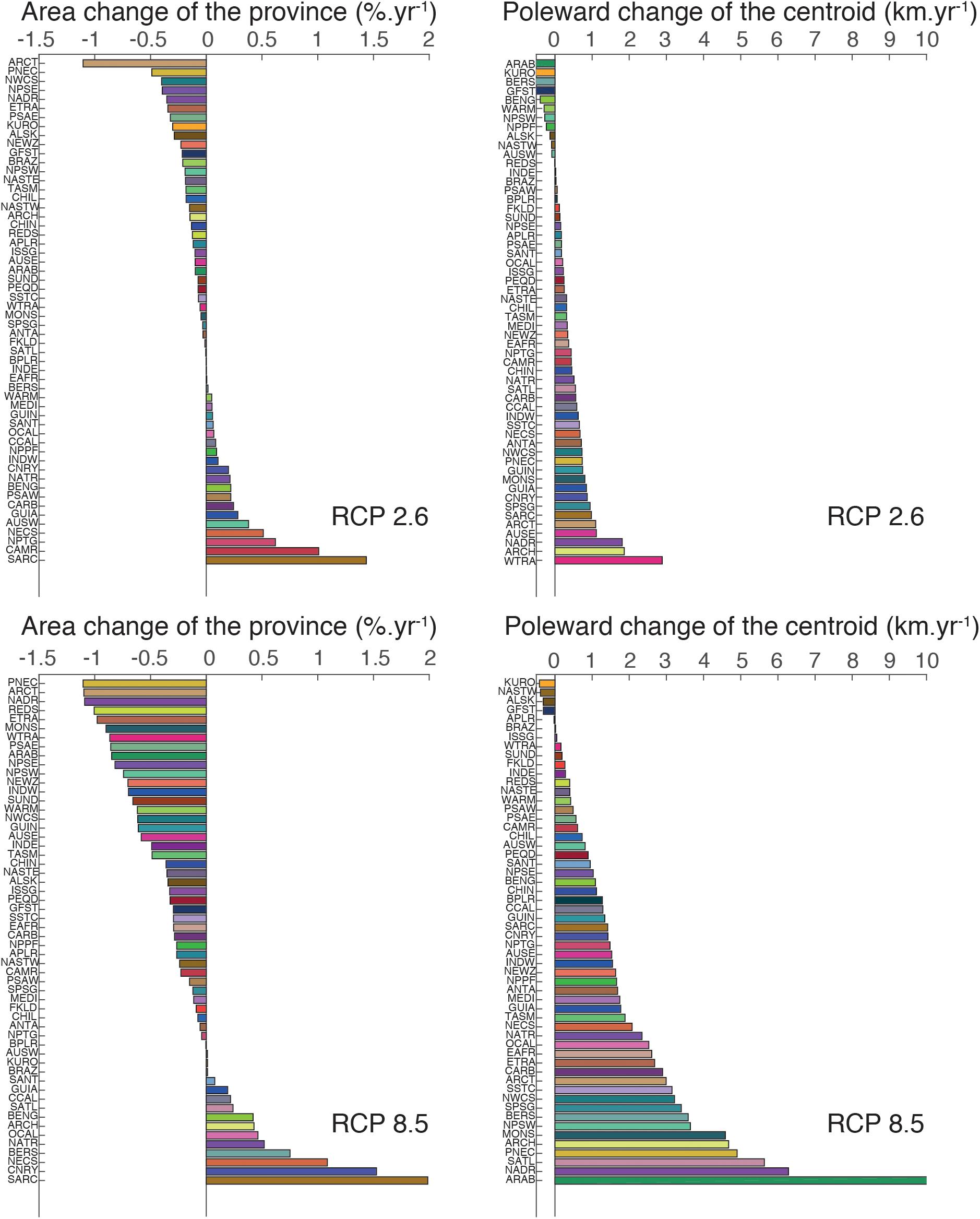
Figure 2. Bar plot of the mean latitudinal change of the BGCPs’ centroid (in km.year–1) and percentage of BGCPs area change by 2100 compared to the 1970–2000 reference period (in % .year–1) under RCP 2.6 and 8.5. The color code as well as acronyms are the same as Figure 1A.
We projected significantly higher rates of poleward centroid shifts and changes in total area of the BGCPs under RCP 8.5 compared to RCP 2.6 (Figure 2). The average projected rate of poleward shift across the 56 BGCPs was 0.36 ± 0.66 km.year–1 (average and standard error) and 1.83 ± 1.99 km.year–1 under RCP 2.6 and RCP 8.5, respectively. ARAB (Arabian sea, 10.99 ± 0.81 km.year–1), NADR (North Atlantic Drift Region, 6.28 ± 4.72 km.year–1), and SATL (South Atlantic gyral province, 5.63 ± 3.45 km.year–1) were the BGCPs exhibiting the strongest shift in their centroid (Figure 2). The ARAB shift would translate into a move north up to a 1,180 km by 2100. In contrast, the ISSG (Indian ocean South Subtropical Gyre province)and BRAZ (Brazilian coastal province) BGCPs did not shift, keeping their centroid locations constant (rate of shift of 0.02–0.05 km.year–1). Biogeochemical provinces that were projected to expand the most were SARC (Sub atlantic ARCtic province; 1.98%.year–1), CNRY (1.52%.year–1) and NECS (NorthEast Atlantic Continental Shelve province, 1.08%.year–1) – effectively doubling or more in size by 2100 – while PEQD (Pacific EQuatorial Divergence province, -1.10%.year–1), ARCT (ARCTic province, -11.09%.year–1) and NADR (North Atlantic Drift Region, -11.09%.year–1) were expected to shrink substantially.
To highlight the different categories of spatial changes registered by the BGCPs, we describe here examples of the three classes of projected change BGCPs may undergo: (1) poleward shift (North Atlantic Drift Region, NADR), (2) expansion with no spatial shift (North Atlantic Tropical Region, NATR), and (3) no specific change in size or location (Chilean coast, CHIL) (Figure 3). The probability of occurrence of the NADR province was projected to decrease sharply at the southern portion of its distribution towards the end of the 21st century under RCP 8.5, with the area between the Greenland Sea and Norwegian Sea displaying more NADR-like conditions over the course of this period. Hence, the overall location of this BGCP is projected to shift northward. For NATR (North Atlantic Tropical Region), the BGCP boundary is projected to expand northward and southward into the Atlantic Ocean, while the probability of occurrence of the NATR province shows only a slight decline by the end of the century under RCP 8.5. For the CHIL BGCP, the projected boundary and probability of occurrence remained relatively stable under all scenarios.
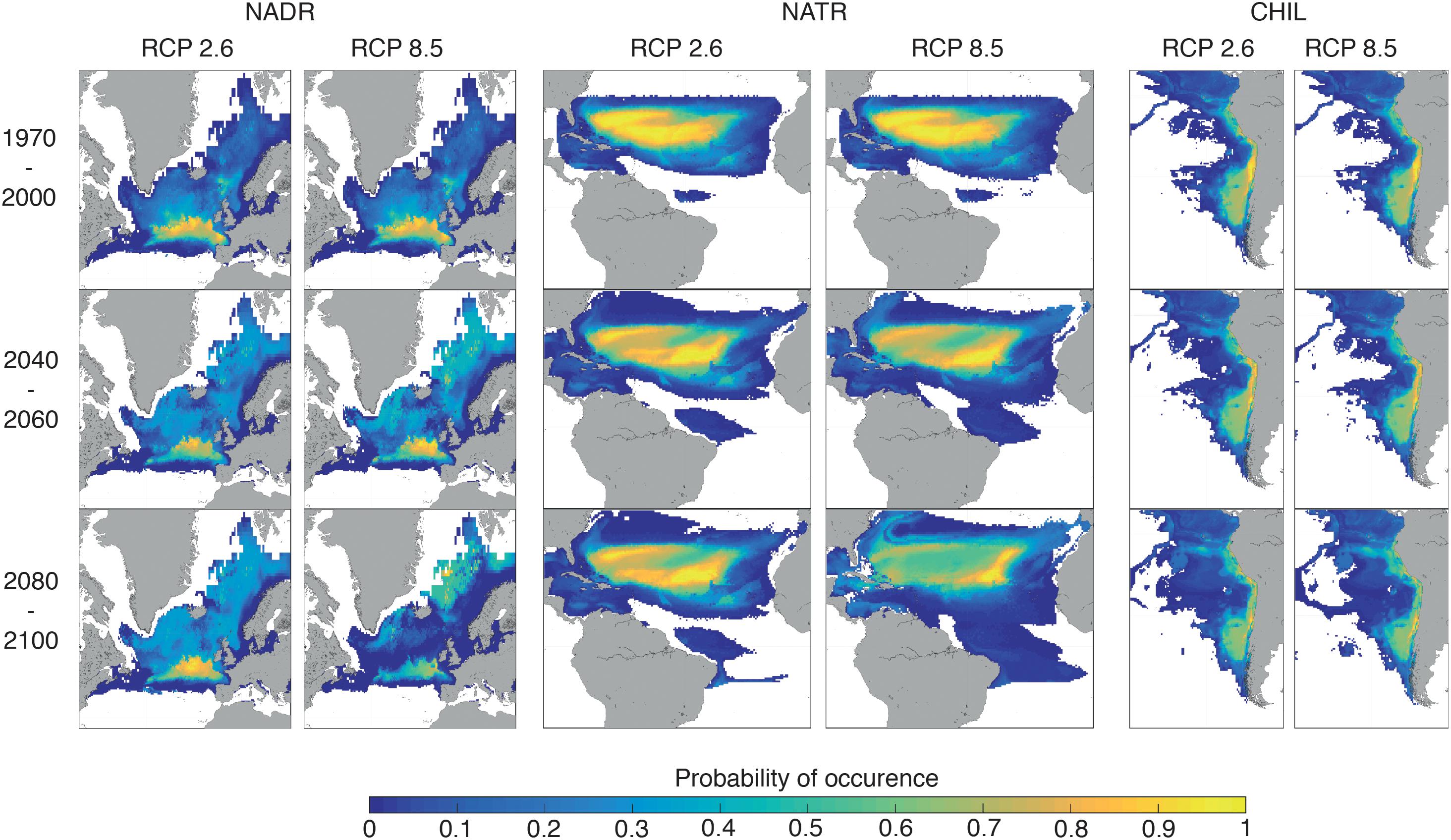
Figure 3. Spatial distribution of the probability of occurrence of the following three BGCPs: North Atlantic Drift region (NADR), North Atlantic Tropical Region (NATR) and Chilean coast (CHIL). Mean ESMs and ENMs distribution of each province for the period 1970–2000, 2040–2060, and 2080–2100 are represented for both RCP 2.6 and 8.5.
We identified the emergence of a NABS in large areas of the western tropical Pacific Ocean, eastern tropical Indian Ocean and eastern tropical Atlantic Ocean (Figure 4). The earliest emergence of a NABS region (across all 3 ESMs) was projected to occur in the tropical south Pacific Ocean in the 2040s, under RCP 8.5. This NABS region was projected to grow very rapidly during the 2050s and 2060s, extending into the eastern Indian Ocean and emerging off the coast of tropical west Africa in the 2070s and in the Caribbean in the 2080s. In contrast, under RCP 2.6, the emergence of NABS occurs on average one decade later than under RCP 8.5 in the same general areas. NABS projected size by the end of the 21st century is on average 11.9% of projections under RCP 8.5. NABS regions are characterized by high SST, low oxygen concentration and low NPP or low pH and low NPP conditions compare to the reference period (Supplementary Figure 3).
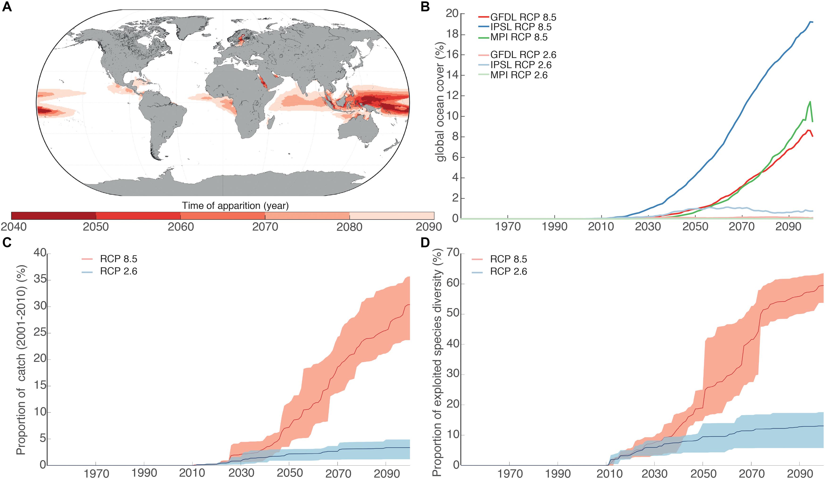
Figure 4. (A) Spatial distribution of the average time of appearance of the NABS across ESMs under RCP 8.5. (B) Evolution of the global coverage of the NABS for the three ESMs and two RCPs. (C) Proportion of global fisheries catches (sum of catch between 2001 and 2010) located in the NABS regions for the period 1970–2100. Interval of confidence computed using the three different ESMs. Thick line represents the median across ESMs. (D) Proportion of the number of species in the NABS for the period 1970–2100. Interval of confidence computed using the three different ESMs. Thick line represents the median across ESMs.
We projected that a substantial proportion of global marine diversity and fisheries catches are presently located in regions where NABS are projected to develop. Under RCP 8.5, 18.97 ± 6.05% in 2050 and 59.49 ± 4,08% in 2100 of the total number of exploited marine species considered here (N = 1,105 species) will be exposed to the expansion of NABS regions. These NABS regions are indeed projected to develop in areas with high seafood dependence [in terms of calories and nutrition (Golden et al., 2016)] with relatively low adaptive capacity (Blasiak et al., 2017) and high exposure to simultaneous losses in terrestrial food production capacity. The proportion of global marine fisheries catches (average between 2001-2011) caught in areas of predicted NABS in 2050 and 2100 are 7.87 ± 3.94% and 30.39 ± 5.32%, respectively, under RCP 8.5. The projected exposure to NABS was much lower under RCP 2.6, with only 15% of exploited species and 5% of total catch in NABS areas by the end of the 21st century. The difference in trajectories in regards to NABS between RCP 2.6 and RCP 8.5 became significantly larger than the inter-ESM variability after the end of the 2040s.
Discussion
This study supports the hypotheses that climate change will deeply affect the biogeography of the global ocean, and lead to the emergence of biomes with no historical analog. At the global scale, we predict that trade wind provinces will expand (Staten et al., 2018), with the distribution of several westerly wind provinces migrating poleward. This evolution will be driven mostly by the poleward extension of warm surface waters, pH, oxygen concentration, and NPP (Supplementary Figure 2). Warming of the tropics will drive a poleward migration of the BGCPs (Figure 1 and Supplementary Figure 2) with the polar provinces progressively shrinking over time and being concentrated at the highest latitudes. These biogeographical changes appear to be corroborated by the rapid modifications in biogeochemical processes, species composition and food web dynamics already documented for these regions (Beaugrand et al., 2002; Dulvy et al., 2008; Polovina et al., 2008; Stramma et al., 2012; Fossheim et al., 2015). Such patterns are also in accordance with other projections performed using modeled distributions of marine species (Cheung et al., 2009; Lenoir et al., 2011), biomes (Sarmiento et al., 2004) and climate velocity computed using only SST(Burrows et al., 2011). However, in areas where province boundaries are constrained by the presence of land, we expect a significant decline in the original area of several provinces (ARAB, GUIN, GUIA, CARB, CHIN), with the potential to significantly impact the ecological assemblages characterizing those provinces.
Our results show that NABS regions will cover areas where a substantial proportion of global marine biodiversity presently occurs and with a crucial dependence on seafood production. The emergence of wide NABS areas in the tropical ocean will exacerbate the high vulnerability of populations living in developing coastal nations and small island states (Lam et al., 2016; Blasiak et al., 2017). Biodiversity, structure and function of marine ecosystems, and fisheries catches are closely related to the characteristics of the BGCPs (Reygondeau et al., 2013). The climate-induced changes to BGCPs that we project provide additional support to the idea that climate change will deeply alter the distribution and function of marine ecosystems as well as the benefits derived from them by people. Predicting the evolution of marine biodiversity in the NABS areas raises significant challenges, as the knowledge we currently hold regarding the organization of ecosystems in existing biomes is likely to be invalidated in no-analog environmental conditions (Fitzpatrick and Hargrove, 2009). While we cannot definitively state that no species stand to benefit from these new conditions, as the NABS predominantly occur in tropical regions where many species are already close to physiological maxima (Walther et al., 2002; Sunday et al., 2011, 2012), it is likely the emergence of NABS will substantially elevate the risk of impacts on marine biodiversity and fisheries.
The NABS were characterized by very warm mean annual temperatures, high salinity, low oxygen concentration and low NPP compared to the reference period (Supplementary Figure 3). Most marine species will be physiologically stressed under such conditions, which could impact their survival rate (Sunday et al., 2012). This explains the high rate of local extinction predicted by previous studies in the regions where NABS environmental conditions will not fit the environmental tolerance range of the majority of endemic species (Beaugrand et al., 2015; Jones and Cheung, 2015). Paleontological records have shown that the apparition of novel types of climate increases the rate of migration impacting the local biodiversity pool (Jablonski, 2008). Also, such changes in the local environmental condition will impact the biological processes of marine species. In NABS regions, we therefore expect a decrease in the size of endemic species as well as a decline in local biomass, as suggested by the literature. However, it is possible that some species will manage to survive in NABS-like environments, particularly small organisms with high turnover rates, such as microbes, that have good potential for rapid adaptation, as well as species that are physiologically more flexible, such as widely distributed marine species that occur in the Pacific Warm Pool. However, species that prove capable of adapting in NABS may only represent a small fraction of the currently high biological diversity occurring in these regions (Donelson et al., 2019; Palumbi et al., 2019).
Our results can be linked to recent studies on marine extreme events (Frölicher et al., 2018; Oliver et al., 2018) that have shown, using satellite observations, that recurring and permanent marine heatwaves already occur in the regions where we expect NABS to appear by the middle of the 21st century. We can reasonably expect that the impacts that these marine heatwaves already have had on marine life (Le Nohaïc et al., 2017; Oliver et al., 2017) will be similar or even amplified under NABS conditions. The emergence of NABS would be limited in most regions of the global ocean if CO2 emissions can be held to the level required to achieve RCP 2.6 (Figure 1). However, if this is not the case (which currently appears likely), we expect the earliest NABS to emerge in about twenty years from 2010 in the tropical Pacific region and a decade later in the Indo-Pacific basin. There is therefore an urgent need to develop adaptation policies anticipating the risk of rapid ecosystem collapses in these regions, in addition to supporting efforts for strong mitigation.
The original methodology developed in Reygondeau et al. (2013) was applied on observed environmental data and used the ocean partition proposed by Longhurst (2007) as framework to quantify the environmental envelopes of BGCPs. Consequently, the application of the methodology to ESM have large uncertainty in correctly representing the ocean properties in several regions of the Ocean and hence distribution of BGCPs. The natural provinces (or regions of similar environmental conditions) derived from the models may not spatially match the prescribed boundaries found in Reygondeau et al. (2013). We subsequently tested the spatial and temporal agreement between our predictions based on different ESM projections and results from Reygondeau et al. (2013) (Supplementary Figure 1). Overall, the spatial division and internal variation of BGCPs are well captured in ESM outputs (Supplementary Figure 1), but several regions need to be considered with caution. First, the dynamic of coastal regions are not well captured by this generation of ESMs in the CMIP5 repository (Stock et al., 2011; Cheung et al., 2016a) and consequently, the distribution and dynamics of coastal BGCPs are not well represented for current or future projection. Second, semi enclosed sea (Red sea, Persian Gulf, Baltic sea, Mediterranean sea) have similar biases as coastal regions and results for these areas need to be taken with caution. Third, while the division of the southern ocean is well captured by the methodology using ESM outputs, several biases in the representation of the region biogeochemical dynamics are known (Bindoff et al., 2019). Consequently, future projection of the BGCPs in the southern Ocean are sensitive to thse biases. We hope that the finer resolution of the new generation of ESM models that are under development may resolve these issues in a future re-analysis.
Our results indicate that the environmental changes that would occur in the global ocean along a “no mitigation” RCP 8.5 scenario would lead to a drastic reorganization of global marine biogeography, associated biodiversity and trophic networks. These changes would include the emergence of wide regions with no environmental analog compared to current observations. If the global climate is not kept below 2°C warming, NABS areas can be expected to emerge, as early as 20 years from the 2010s. It would affect 19% of the total number of exploited species in 2050 and 59% in 2100 and would cover regions that are currently responsible for 8% of global marine fisheries catch in 2050 and 30% in 2100, under RCP 8.5. These numbers would change to only 15% of exploited species and 5% of total fisheries catches in NABS areas by the end of the 21st century under the RCP 2.6 scenario. Mitigating anthropogenic pressures at a level sufficient to reach the Paris agreement targets would therefore substantially reduce the risk of emergence of large NABS regions in the global ocean, and the dramatic consequences that such large-scale ecological changes would entail for tropical marine biodiversity, associated fisheries and the human communities that they support.
Data Availability Statement
The datasets generated for this study are available on request to the corresponding author.
Author Contributions
GR performed all the analyses and wrote the original of the manuscript. Idea originated from OM and GR. All other co-authors contributed to data sharing, idea, analysis, and writing of the manuscript. All authors contributed to the article and approved the submitted version.
Funding
WC, GR, CW, and VL acknowledge funding support from the Nippon Foundation-the University of British Columbia Nereus Program. WC acknowledges support from the Natural Sciences and Engineering Research Council of Canada. OM acknowledges the support of the French ANR project CIGOEF (grant ANR-17-CE32-0008-01). TF thanks the Swiss National Science Foundation (PP00P2_170687) and the European Union’s Horizon 2020 Research and Innovation Programme under grant agreement no. 820989 (project COMFORT, Our common future ocean in the Earth system – quantifying coupled cycles of carbon, oxygen, and nutrients for determining and achieving safe operating spaces with respect to tipping points) for financial support.
Conflict of Interest
The authors declare that the research was conducted in the absence of any commercial or financial relationships that could be construed as a potential conflict of interest.
Acknowledgments
This study is dedicated by GR to the memory of Madeleine Remy.
Supplementary Material
The Supplementary Material for this article can be found online at: https://www.frontiersin.org/articles/10.3389/fmars.2020.00657/full#supplementary-material
Footnotes
References
Asch, R. G., Cheung, W. W. L., and Reygondeau, G. (2017). Future marine ecosystem drivers, biodiversity, and fisheries maximum catch potential in Pacific Island countries and territories under climate change. Mar. Policy. 88, 285–294. doi: 10.1016/j.marpol.2017.08.015
Beaugrand, G., Edwards, M., Raybaud, V., Goberville, E., and Kirby, R. R. (2015). Future vulnerability of marine biodiversity compared with contemporary and past changes. Nat. Clim. Chang 5, 695–701. doi: 10.1038/nclimate2650
Beaugrand, G., Lenoir, S., Ibañez, F., and Manté, C. (2011). A new model to assess the probability of occurrence of a species, based on presence-only data. Mar. Ecol. Prog. Ser. 424, 175–190. doi: 10.3354/meps08939
Beaugrand, G., Reid, P., Ibañez, F., and Planque, B. (2000). Biodiversity of North Atlantic and North Sea calanoid copepods. Mar. Ecol. Prog. Ser. 204, 299–303. doi: 10.3354/meps204299
Beaugrand, G., Reid, P. C., Ibañez, F., Lindley, J. A., and Edwards, M. (2002). Reorganization of North Atlantic marine copepod biodiversity and climate. Science 296, 1692–1694. doi: 10.1126/science.1071329
Bindoff, N. L., Cheung, W. W. L., Kairo, J. G., Arístegui, J., Guinder, V. A., Hallberg, R., et al. (2019). “Changing ocean, marine ecosystems, and dependent communities,” in IPCC Special Report on the Ocean and Cryosphere in a Changing Climate, eds H.-O. Pörtner, D. C. Roberts, V. Masson-Delmotte, P. Zhai, M. Tignor, E. Poloczanska, et al. Available online at: https://www.researchgate.net/publication/341281995_Changing_Ocean_Marine_Ecosystems_and_Dependent_Communities_09_SROCC_Ch05_FINAL-1 (accessed September 28, 2020).
Blasiak, R., Spijkers, J., Tokunaga, K., Pittman, J., Yagi, N., and Österblom, H. (2017). Climate change and marine fisheries: Least developed coutries top global index of vulnerability. PLoS One. 12:e0179632. doi: 10.1371/journal.pone.0179632
Burrows, M. T., Schoeman, D. S., Buckley, L. B., Moore, P., Poloczanska, E. S., Brander, K. M., et al. (2011). The pace of shifting climate in marine and terrestrial ecosystems. Science 334, 652–655. doi: 10.1126/science.1210288
Chassot, E., Bonhommeau, S., Reygondeau, G., Nieto, K., Polovina, J. J., Huret, M., et al. (2011). Satellite remote sensing for an ecosystem approach to fisheries management. ICES J. Mar. Sci. J. du Cons. 68:651.
Cheung, W. W. L. (2018). The future of fishes and fisheries in the changing oceans. J. Fish Biol. 92, 790–803. doi: 10.1111/jfb.13558
Cheung, W. W. L., Jones, M. C., Reygondeau, G., Stock, C. A., Lam, V. W. Y., and Frölicher, T. L. (2016a). Structural uncertainty in projecting global fisheries catches under climate change. Ecol. Modell. 325, 57–66. doi: 10.1016/j.ecolmodel.2015.12.018
Cheung, W. W. L., Reygondeau, G., and Frölicher, T. L. (2016b). Large benefits to marine fisheries of meeting the 1.5°C global warming target. Science 354, 1591–1594. doi: 10.1126/science.aag2331
Cheung, W. W. L., Lam, V. W. Y., Sarmiento, J. L., Kearney, K., Watson, R., and Pauly, D. (2009). Projecting global marine biodiversity impacts under climate change scenarios. Fish Fish. 10, 235–251. doi: 10.1111/j.1467-2979.2008.00315.x
de Boyer Montégut, C., Madec, G., Fischer, A. S., Lazar, A., and Ludicone, D. (2004). Mixed layer depth over the global ocean: An examination of profile data and a profile-based climatology. J. Geophys. Res. C 109, C12003.
Demarcq, H., Reygondeau, G., Alvain, S., and Vantrepotte, V. (2012). Monitoring marine phytoplankton seasonality from space. Remote Sens. Environ. 117, 211–222. doi: 10.1016/j.rse.2011.09.019
Donelson, J. M., Sunday, J. M., Figueira, W. F., Gaitán-Espitia, J. D., Hobday, A. J., Johnson, C. R., et al. (2019). Understanding interactions between plasticity, adaptation and range shifts in response to marine environmental change. Philosoph. Transact. Royal Soc. B 374:20180186.
Dulvy, N. K., Rogers, S. I., Jennings, S., Stelzenmller, V., Dye, S. R., and Skjoldal, H. R. (2008). Climate change and deepening of the North Sea fish assemblage: a biotic indicator of warming seas. J. Appl. Ecol. 45, 1029–1039. doi: 10.1111/j.1365-2664.2008.01488.x
Elith, J., Leathwick, J. R., and Hastie, T. (2008). A working guide to boosted regression trees. J. Anim. Ecol. 77, 802–813. doi: 10.1111/j.1365-2656.2008.01390.x
Fitzpatrick, M. C., and Hargrove, W. W. (2009). The projection of species distribution models and the problem of non-analog climate. Biodivers. Conserv. 18:2255. doi: 10.1007/s10531-009-95849588
Fossheim, M., Primicerio, R., Johannesen, E., Ingvaldsen, R. B., Aschan, M. M., and Dolgov, A. V. (2015). Recent warming leads to a rapid borealization of fish communities in the Arctic. Nat. Clim. Chang. 5, 673–677. doi: 10.1038/nclimate2647
Froelicher, T. L., Rodgers, K. B., Stock, C. A., and Cheung, W. W. L. (2016). Sources of uncertainties in 21st century projections of potential ocean ecosystem stressors. Global Biogeochem. Cycles. 30, 1224–1243. doi: 10.1002/2015GB005338
Frölicher, T. L., Fischer, E. M., and Gruber, N. (2018). Marine heatwaves under global warming. Nature 560, 383–389. doi: 10.1038/s41586-018-0383389
Gagné, T. O., Reygondeau, G., Jenkins, C. N., Sexton, J. O., Bograd, S. J., Hazen, E. L., et al. (2020). Towards a global understanding of the drivers of marine and terrestrial biodiversity. PLoS One 15:e0228065. doi: 10.1371/journal.pone.0228065
Gattuso, J. P., Magnan, A., Billé, R., Cheung, W. W. L., Howes, E. L., Joos, F., et al. (2015). Contrasting futures for ocean and society from different anthropogenic CO2emissions scenarios. Science 349:aac4722. doi: 10.1126/science.aac4722
Golden, C. D., Allison, E. H., Cheung, W. W. L., Dey, M. M., Halpern, B. S., McCauley, D. J., et al. (2016). Nutrition: Fall in fish catch threatens human health. Nature 534, 317–320. doi: 10.1038/534317a
Jablonski, D. (2008). Extinction and the spatial dynamics of biodiversity. Proc. Natl. Acad. Sci. 1, 11528–11535. doi: 10.1073/pnas.0801919105
Jones, M. C., and Cheung, W. W. L. (2015). Multi-model ensemble projections of climate change effects on global marine biodiversity. ICES J. Mar. Sci. 72, 741–752. doi: 10.1093/icesjms/fsu172
Kavanagh, P., Newlands, N., Christensen, V., and Pauly, D. (2004). Automated parameter optimization for Ecopath ecosystem models. Ecol. Modell. 172, 141–149.
Lam, V. W. Y., Cheung, W. W. L., Reygondeau, G., and Rashid Sumaila, U. (2016). Projected change in global fisheries revenues under climate change. Sci. Rep. 6:32607. doi: 10.1038/srep32607
Le Nohaïc, M., Ross, C. L., Cornwall, C. E., Comeau, S., Lowe, R., McCulloch, M. T., et al. (2017). Marine heatwave causes unprecedented regional mass bleaching of thermally resistant corals in northwestern Australia. Sci. Rep. 7:14999. doi: 10.1038/s41598-017-14794-y
Lenoir, S., Beaugrand, G., and Lécuyer, E. (2011). Modeled spatial distribution of marine fish and projected modifications in the North Atlantic Ocean. Glob. Chang. Biol. 17, 115–129. doi: 10.1111/j.1365-2486.2010.02229.x
Morel, A., Huot, Y., Gentili, B., Werdell, P. J., Hooker, S. B., and Franz, B. A. (2007). Examining the consistency of products derived from various ocean color sensors in open ocean (Case 1) waters in the perspective of a multi-sensor approach. Remote Sens. Environ. 111, 69–88. doi: 10.1016/j.rse.2007.03.012
Oliver, E. C. J., Benthuysen, J. A., Bindoff, N. L., Hobday, A. J., Holbrook, N. J., Mundy, C. N., et al. (2017). The unprecedented 2015/16 Tasman Sea marine heatwave. Nat. Commun. 8, 1–12. doi: 10.1038/ncomms16101
Oliver, E. C. J., Donat, M. G., Burrows, M. T., Moore, P. J., Smale, D. A., Alexander, L. V., et al. (2018). Longer and more frequent marine heatwaves over the past century. Nat. Commun. 9:1324. doi: 10.1038/s41467-018-037323739
Oliver, M. J., and Irwin, A. J. (2008). Objective global ocean biogeographic provinces. Geophys. Res. Lett. 35:L15601.
Palumbi, S. R., Evans, T. G., Pespeni, M. H., and Somero, G. N. (2019). Present and future adaptation of marine species assemblages. Oceanography 32, 82–93.
Peel, M. C., Finlayson, B. L., and Mcmahon, T. A. (2007). Updated world map of the Koppen-Geiger climate classification. Hydrol. Earth Syst. Sci. Discuss. 11, 1633–1644. doi: 10.1127/0941-2948/2006/0130
Phillips, S. J., Dudík, M., and Schapire, R. E. (2004). “A maximum entropy approach to species distribution modeling,” in Proceedings of the twenty-first international conference on Machine learning, (New York: ACM), 83.
Polovina, J. J., Howell, E. A., and Abecassis, M. (2008). Ocean’s least productive waters are expanding. Geophys. Res. Lett. 35, 1–5.
Reygondeau, G., Longhurst, A., Martinez, E., Beaugrand, G., Antoine, D., and Maury, O. (2013). Dynamic biogeochemical provinces in the global ocean. Global. Biogeochem. Cycles 27, 1046–1058.
Reygondeau, G., Maury, O., Beaugrand, G., Fromentin, J. M., Fonteneau, A., and Cury, P. (2012). Biogeography of tuna and billfish communities. J. Biogeogr. 39, 114–129. doi: 10.1111/j.1365-2699.2011.02582.x
Sarmiento, J. L., Slater, R., Barber, R., Bopp, L., Doney, S. C., Hirst, A. C., et al. (2004). Response of ocean ecosystems to climate warming. Global Biogeochem. Cycles. 18:GB3003. doi: 10.1029/2003GB002134
Sayre, R., Dangermond, J., Frye, C., Vaughan, R., Aniello, P., Breyer, S., et al. (2014). A New Map of Global Ecological Land Units – An Ecophysiographic Stratification Approach. Washington, DC: Association of American Geographers, 46.
Smith, W. H. F., and Sandwell, D. T. (1997). Global Sea Floor Topography from Satellite Altimetry and Ship Depth Soundings. Science 277, 1956–1962.
Staten, P. W., Lu, J., Grise, K. M., Davis, S. M., and Birner, T. (2018). Re-examining tropical expansion. Nat. Clim. Chang. 8, 768–775. doi: 10.1038/s41558-018-0246242
Stock, C. A., Alexander, M. A., Bond, N. A., Brander, K. M., Cheung, W. W. L., Curchitser, E. N., et al. (2011). On the use of IPCC-class models to assess the impact of climate on living marine resources. Prog. Oceanogr. 88, 1–27.
Stramma, L., Prince, E. D., Schmidtko, S., Luo, J., Hoolihan, J. P., Visbeck, M., et al. (2012). Expansion of oxygen minimum zones may reduce available habitat for tropical pelagic fishes. Nat. Clim. Chang. 2, 33–37. doi: 10.1038/nclimate1304
Sunday, J. M., Bates, A. E., and Dulvy, N. K. (2011). Global analysis of thermal tolerance and latitude in ectotherms. Proc. R. Soc. B Biol. Sci. 278, 1823–1830. doi: 10.1098/rspb.2010.1295
Sunday, J. M., Bates, A. E., and Dulvy, N. K. (2012). Thermal tolerance and the global redistribution of animals. Nat. Clim. Chang. 2, 686–690. doi: 10.1038/nclimate1539
Taylor, K. E., Stouffer, R. J., and Meehl, G. A. (2012). An overview of CMIP5 and the experiment design. Bull. Am. Meteorol. Soc. 93, 485–498. doi: 10.1175/BAMS-D-11-00094.1
Keywords: physical oceanography, marine biogeography, pelagic environment, novel ocean climate, environmental niche model
Citation: Reygondeau G, Cheung WWL, Wabnitz CCC, Lam VWY, Frölicher T and Maury O (2020) Climate Change-Induced Emergence of Novel Biogeochemical Provinces. Front. Mar. Sci. 7:657. doi: 10.3389/fmars.2020.00657
Received: 01 March 2020; Accepted: 20 July 2020;
Published: 15 October 2020.
Edited by:
Kenneth Alan Rose, University of Maryland Center for Environmental Science (UMCES), United StatesReviewed by:
Juan José Morrone, National Autonomous University of Mexico, MexicoScott Doney, University of Virginia, United States
Victoria Janet Coles, University of Maryland Center for Environmental Science (UMCES), United States
Copyright © 2020 Reygondeau, Cheung, Wabnitz, Lam, Frölicher and Maury. This is an open-access article distributed under the terms of the Creative Commons Attribution License (CC BY). The use, distribution or reproduction in other forums is permitted, provided the original author(s) and the copyright owner(s) are credited and that the original publication in this journal is cited, in accordance with accepted academic practice. No use, distribution or reproduction is permitted which does not comply with these terms.
*Correspondence: Gabriel Reygondeau, gabriel.reygondeau@gmail.com