Projected Effects of Climate-Induced Changes in Hydrodynamics on the Biogeochemistry of the Mediterranean Sea Under the RCP 8.5 Regional Climate Scenario
 Rémi Pagès1
  Melika Baklouti1*
  Nicolas Barrier2
  Mohamed Ayache1
  Florence Sevault3
  Samuel Somot3
  Thierry Moutin1
- 1Aix Marseille Université, Université de Toulon, CNRS, IRD, MIO UM 110, Marseille, France
- 2MARBEC, University of Montpellier, CNRS, Ifremer, IRD, Montpellier, France
- 3CNRM, Université de Toulouse, Météo-France, CNRS, Toulouse, France
The Mediterranean region has been shown to be particularly exposed to climate change, with observed trends that are more pronounced than the global tendency. In forecast studies based on a RCP 8.5 scenario, there seems to be a consensus that, along with an increase in temperature and salinity over the next century, a reduction in the intensity of deep-water formation and a shallowing of the mixed layer [especially in the North-Western Mediterranean Sea (MS)] are expected. By contrast, only a few studies have investigated the effects of climate change on the biogeochemistry of the MS using a 3D physical/biogeochemical model. In this study, our aim was to explore the impact of the variations in hydrodynamic forcing induced by climate change on the biogeochemistry of the MS over the next century. For this purpose, high-resolution simulations under the RCP 8.5 emission scenario have been run using the regional climate system model CNRM-RCSM4 including the NEMO-MED8 marine component, coupled (off-line) with the biogeochemical model Eco3M-Med. The results of this scenario first highlight that most of the changes in the biogeochemistry of the MS will occur (under the RCP 8.5 scenario) after 2050. They suggest that the MS will become increasingly oligotrophic, and therefore less and less productive (14% decrease in integrated primary production in the Western Basin and in the Eastern Basin). Significant changes would also occur in the planktonic food web, with a reduction (22% in the Western Basin and 38% in the Eastern Basin) of large phytoplankton species abundance in favor of small organisms. Organisms will also be more and more N-limited in the future since NO3 concentrations are expected to decline more than those of PO4 in the surface layer. All these changes would mainly concern the Western Basin, while the Eastern Basin would be less impacted.
1. Introduction
Since the beginning of the industrial era, a vast amount of greenhouse gases have been released into the atmosphere through human activities. For example, the average atmospheric CO2 concentration, which was around 280 ppm in the pre-industrial era, had reached 408 ppm in 2019 (Dlugokencky and Tans, 2019). These high concentrations of greenhouse gas in the atmosphere have accentuated the natural greenhouse effect and induced a global rise of the temperature of 1°C in 2018 (Allen et al., 2018), leading to major climate changes. However, in some regions, including the Mediterranean region, the temperature rise is expected to be higher than the global increase (Seneviratne et al., 2016) due to local characteristics such as land-use and/or land-cover (Pitman et al., 2009), urban development (Wilby, 2008) or aerosols (Levy et al., 2013).
The Mediterranean region has already been demonstrated to be particularly exposed to climate change by Giorgi (2006). The observed trend for the rate of climate change in the Mediterranean region is indeed higher than the global tendency (Cramer et al., 2018). For example, the average temperature is 1.4°C above the pre-industrial value and heat waves as well as droughts occur more frequently (Cramer et al., 2018). Furthermore, the Mediterranean region is increasingly impacted by human activities, with a population in North Africa that rose 4-fold between 1960 and 2015, while urbanization increased by a factor of 2 (Cramer et al., 2018). As a semi-enclosed sea surrounded by land and numerous industrialized countries, the Mediterranean sea (MS) is highly sensitive to climate change. Because of the specific response to climate change of the Mediterranean region (and consequently of the MS), there is a need to model climate scenarios at regional scale in order to fully cover the nature and the magnitude of the expected changes in this area.
In the MS, most hydrodynamic studies have predicted a global increase in temperature and salinity during the next century as well as a decline in deep water formation and a shallowing of the Mixed Layer (Somot et al., 2006; Durrieu de Madron et al., 2011; Adloff et al., 2015; Darmaraki et al., 2019). However, it has been shown recently by Soto-Navarro et al. (2020), who analyzed a set of 25 simulations, that the predicted warming is not homogeneous throughout the MS. All the models in this study showed a high rate of warming in the Levantine Basin, the north of the Aegean Sea, the Adriatic Sea, and the Balearic Sea. They also highlighted that despite the overall salinity increase throughout the MS, the surface of the Western Mediterranean Basin (Western Basin) will be mainly impacted by the characteristics of the Atlantic waters inflowing into the Western Mediterranean Basin due to the higher water input of north-eastern Atlantic waters predicted by most general circulation models (GCMs). Finally, Soto-Navarro et al. (2020) pointed out that these changes will probably lead to a reduction in deep water formation in the Gulf of Lions.
The dynamics of the Mixed Layer Depth (MLD) directly affects the planktonic food web through the availability of their essential nutrients [Nitrate (NO3) and Phosphate (PO4)] in the euphotic layer. In the open ocean, the availability of nutrients in the euphotic layer is mainly driven by the exchanges between the nutrient-depleted upper layers and the nutrient-rich deep layers through vertical mixing (Broecker and Peng, 1982; Van Den Broeck et al., 2004). In the mid-latitude areas (like the MS), the seasonal dynamics of the MLD is mainly responsible for these exchanges (Williams, 2003; Auger et al., 2014). In the MS, between May and November, the MLD is shallow and strong stratification separates the upper layers from the deep layers (Lionello et al., 2006). From December to April, because of strong winds and low temperatures that induce the vertical mixing of the water column, the MLD becomes deeper (Houpert et al., 2015). This process allows the homogenization of the water mass above the MLD and injects nutrients into the upper layers.
To our knowledge, only a few studies have investigated the effects of climate change on the biogeochemistry of the whole MS with a 3D coupled hydrodynamic/biogeochemical model. Most of those studies, except Moullec et al. (2019), have predicted a decline in primary production for the Western Basin and nutrient inputs to the upper layers due to a reduction in vertical mixing (Macias et al., 2015; Richon et al., 2019). Some studies also highlight a reduction of the phytoplankton biomass (mostly for diatoms) (Lazzari et al., 2014; Richon et al., 2019), while Moullec et al. (2019) show an increase in phytoplankton biomass. Finally Richon et al. (2019) show a deepening of the deep chlorophyll maximum (DCM) while Macias et al. (2015) show that it will become slightly shallower.
This study is intended to be a further contribution to present knowledge in this field. All these previous studies, except that of Lazzari et al. (2014), use a fixed stochiometry for some or all of the unicellular plankton functional types in the model. Moreover, some of these studies use discontinuous (i.e. not all the period has been simulated) simulations (Lazzari et al., 2014) and/or old SRES climate change scenarios (Lazzari et al., 2014; Richon et al., 2019). Furthermore, due to the scarcity of available data, all of them used rivers' nutrient inputs that are not consistent with the scenario used, and this is also the case for the present study.
Here we present the first study based on a biogeochemical model that considers a flexible stoichiometry for all the Plankton Functional Types (PFTs) (with the exception of copepods), and that also calculates the abundance of each PFT.
Furthermore, apart from considerations regarding the structure of the biogeochemical model, the biogeochemistry of the MS in the next century will be driven by the hydrodynamics of the MS, as well as by the input of nutrients at the different boundaries (i.e., inputs of nutrients by rivers, through the Gibraltar Strait, or by atmospheric deposition). In this study, our aim is to focus on the effects of the variations (expected according to the RCP 8.5 scenario) in hydrodynamics alone, apart from the effects induced by future changes in the inputs at the different boundaries. The reasons for this choice are related to our aim of exploring the relative weight of each of the internal and external contributions to the future changes in the MS. This choice also has the advantage of avoiding the uncertainties associated with the evolution of the external forcings (see the Discussion section for more details).
For this purpose, high-resolution simulations over the 1985–2100 period have been run using the Eco3M-Med biogeochemical model forced by the RCP 8.5 emission scenario for the twenty-first century provided by the high-resolution and fully-coupled regional climate system model CNRM-RCSM4 (Sevault et al., 2014; Darmaraki et al., 2019), while nutrient inputs by rivers and through Gibraltar Strait were kept unchanged.
2. Materials and Methods
2.1. The Biogeochemical Model: Eco3M-Med
The biogeochemical model used in this study is the Eco3M-Med configuration (Alekseenko et al., 2014; Guyennon et al., 2015; Pagès et al., 2020). It is coupled off-line with the hydrodynamical model NEMO (Nucleus for European Modeling of the Ocean, Madec and NEMO-Team, 2016). It is embedded in the Ecological Mechanistic and Modular Modeling (Eco3M) tool for biogeochemical modeling (Baklouti et al., 2006a) which is based, as far as possible, on mechanistic descriptions of biogeochemical fluxes (Baklouti et al., 2006b; Mauriac et al., 2011; Alekseenko et al., 2014; Guyennon et al., 2015).
The Eco3M-Med configuration has been designed to represent the main characteristics of the MS. It includes six different plankton functional types (PFTs), two phytoplankton compartments, one large phytoplankton (PHYL) (i.e., phytoplankton with size above 10 μm) and one small phytoplankton (PHYS) (i.e., phytoplankton with size below 10 μm), three zooplankton compartments, the copepods (COP), the ciliates (CIL) and the heterotrophic nanoflagellates (HNF) as well as a compartment of heterotrophic bacteria (BAC). Three pools of inorganic matter are also represented, namely nitrate (NO3), ammonium (NH4), and phosphate (PO4) as well as a pool of dissolved organic matter (DOM) and two compartments of detrital particulate matter, one with small particles (DETS) and the other with large particles (DETL). More information about the Eco3M-Med configurations is available in Guyennon et al. (2015) and Pagès et al. (2020).
As in the previous versions of the Eco3M-Med model, the intracellular ratios [QXY, where X and Y either stand for nitrogen (N), phosphorus (P) or carbon (C)] in organisms, as well as their cell quotas QX (intracellular quantity of X per cell) are flexible and dynamically calculated by the model. These intracellular ratios and quotas are used to regulate the different biogeochemical fluxes represented by the model. As already mentioned in several previous papers, the use of abundances in addition to biomass to characterize PFTs offers, among other advantages, the opportunity to calculate intracellular quotas which are absolute values giving access to the actual degree of limitation of organisms by each nutrient. More details on these aspects of the model can be found in Alekseenko et al. (2014), Guyennon et al. (2015), and Pagès et al. (2020).
Another important feature of this version of Eco3M-MED is that phytoplankton can directly uptake dissolved organic phosphorus (DOP). In this way, we implicitly consider the DOP hydrolysis by extracellular enzymes (i.e., alkaline phosphatase, nucleotidase, polyphosphatase, or phospho-diesterase) produced by heterotrophic bacteria in depleted conditions (Perry, 1972, 1976; Vidal et al., 2003), thereby making the hydrolyzed DOP also available for phytoplankton.
Finally, in the Eco3M-MED model, there is no regulation of kinetics by temperature. The use of PFTs enables us not only to include implicitly marine diversity in a simplified way (Leblanc et al., 2012), but also to implicitly consider that each external temperature will correspond to the optimum temperature of a given species inside each PFT. However, some minor changes since the version used in Pagès et al. (2020) have been made, since the previous version failed to reproduce the well-marked Deep Chlorophyll Maximum (DCM) in the Eastern Basin. To overcome this issue, the maximum CHL:C ratio has been correlated with available light and more specifically with photosynthetically available radiation (PAR), thereby allowing more efficient photo-acclimation in the model, as given by Equation (1):
As expected, the DCM intensities were stronger, especially in the Eastern Basin, which resulted in a significantly larger quantity of large DETL particles produced at the DCM depth. Since the latter sink at a rate of 50 m per day, it was necessary to reduce their turnover time (from 15 to 1 day) to avoid DETL accumulation in deep waters and too rapid changes in nutrient concentrations at depth.
2.2. The Physical Forcing: CNRM-RCSM4
In this study, the physical forcings of the biogeochemical Eco3M-Med model come from a 1950–2100 scenario simulation performed with the fully-coupled high-resolution Regional Climate System Model CNRM-RCSM4 dedicated to the study of the Mediterranean climate and Mediterranean Sea (Sevault et al., 2014).
The CNRM-RCSM4 simulates the main components of the Mediterranean regional climate system and their interactions. It includes four different components: (I) The atmospheric regional model ALADIN-Climate (Radu et al., 2008; Colin et al., 2010; Herrmann et al., 2011) characterized by a 50 km horizontal resolution, 31 vertical levels, and a time step of 1800 s, (II) the ISBA (Interaction between Soil Biosphere and Atmosphere) land-surface model (Noilhan and Mahfouf, 1996) at a 50 km horizontal resolution, (III) the TRIP (Total Runoff Integrating Pathways) river routine model (Oki and Sud, 1998), which is used to convert the runoff simulated by ISBA into rivers at a 50 km horizontal resolution (Decharme et al., 2010; Szczypta et al., 2012; Voldoire et al., 2013), and (IV) the Ocean general circulation model NEMO (Nucleus for European Modeling of the Ocean, Madec and NEMO-Team, 2016) in its NEMO-MED8 regional configuration (Beuvier et al., 2010). NEMO-MED8 is characterized by a horizontal resolution of 1/8° (grid cells size from 6 to 12 km), a vertical resolution of 43 vertical levels (cell height ranging from 6 to 200 m), and a time step of 1200 s. It covers the MS and a buffer zone (from 11 to 6°W) including part of the Atlantic ocean where boundary conditions are applied for temperature and salinity. Note that the rivers runoffs are fully coupled owing to the TRIP component. This means that freshwater inputs to NEMO-MED8 vary during the simulation according to precipitation and evapotranspiration over land. More details about the CNRM-RCSM4 model can be found in Sevault et al. (2014).
The physical simulation used in the current study is a projection simulation performed with CNRM-RCSM4 under the socio-economic scenario RCP 8.5 and described in Darmaraki et al. (2019). The simulation was run after 130 years of spin-up allowing us to stabilize the model state. The initial conditions came from MEDATLAS-II (Rixen et al., 2005) and the lateral boundary conditions for the atmosphere and ocean regional models came from a RCP 8.5 scenario simulation performed with the CNRM-CM5 General Circulation Model (Voldoire et al., 2013) participating in the CMIP5 multi-model exercise. The physical simulation is divided into two periods: a historical period from 1950 to 2005 and a scenario period from 2006 to 2100, here using the RCP 8.5 IPCC emission scenario. In order to ensure a present-climate state closer to observations, we applied two bias corrections constant in time during the CNRM-RCSM4 simulation: (1) to the atmosphere heat fluxes provided to the ocean by the atmosphere component of the regional coupled model and (2) to the near-Atlantic temperature and salinity 3D oceanic conditions provided by the driving GCM CNRM-CM5 (see Supplementary Material of Soto-Navarro et al., 2020 for more information). In addition we performed a control simulation with CNRM-RCSM4 parallel to the projection run (not shown) in order to verify the model stability. This simulation has already been used by Darmaraki et al. (2019) to study to occurrence of marine heat waves during the next century, by Moullec et al. (2019) to investigate the effect of climate change on the trophic web of the MS (end to end model) and by Soto-Navarro et al. (2020) to study the evolution of the seawater properties during the next century.
2.3. Characteristics of the Simulations
In this study, we ran two simulations with Eco3M-Med. The first simulation is a control covering only the 2006–2100 period. The second simulation includes a historical period between 1985 and 2005 and a scenario period between 2006 and 2100. The control simulation was run in order to ensure that the biogeochemical model does not significantly drift over the scenario period. The configuration of the control simulation is similar to the scenario simulation except for the hydrodynamic forcing, which has been built from the random draw of years among the historical period (1985–2005). To cover the 2006–2100 period we proceeded to several random samplings of 20 years without replacement into the historical period in order to remove any trend present in the historical period. The goal is to simulate a permanent and random present-climate state.
The initial conditions for the biogeochemical model come from the outputs of the hindcast simulation of Pagès et al. (2020) obtained in 1985. This simulation used almost the same biogeochemical model as the present one but with a different spatial resolution (1/12° instead of 1/8°). An additional 10-year spin-up has then been run (years 1985–1990 have been run twice).
Concerning nutrients input at the Gibraltar Strait (the only open boundary), the same procedure as in Pagès et al. (2020) has been applied: climatological data (monthly vertical profiles) were used in the buffer zone (previously defined) for each state variable of the biogeochemical model. The profiles for PO4, NO3, NH4 and for the chlorophyll a concentration (CHL) were extracted from the World Ocean Atlas database while the profiles for the remaining variables were derived from the CHL profiles using conversion factors derived from published works (see Alekseenko et al., 2014 for more details). As already mentioned, nutrients concentrations in the buffer zone remained equal to their climatological monthly values during all runs.
For the rivers inputs, monthly values of NO3 and PO4 have been provided for the 29 main rivers all around the MS by the study of Ludwig et al. (2009). These nutrient inputs are available up to the year 2000. Between 2001 and 2100, the amount (in Kt.a−1) of nutrient river inputs of the year 2000 are repeatedly used as already done in Macias et al. (2015). This implies that at rivers mouths, nutrients concentration can slightly vary, but in the end, the input of nutrients remains constant at the scale of the MED.
Finally, three 20-year periods will be distinguished in this paper to analyse the results: the 1986–2005 period denoted HIST, the 2031–2050 period denoted MID, and the 2081–2100 period denoted END.
2.4. Simulation Analyses
All the variables discussed in the following sections are calculated from monthly values through three steps:
(i) For each grid cell and each year, the yearly average is calculated.
(ii) The yearly values are spatially averaged over the Western and the Eastern Basins, excluding coastal areas where the depth is <200 m (see Figure 1) as done for example in Richon et al. (2018) (cf section 3.1).
(iii) These yearly values are averaged over the three 20-year periods, namely: the HIST period (1986–2005), the MID period (2031–2050), and the END period (2081–2100). The standard deviations (SD) provided in Table 1 are computed on the same 20-years periods.
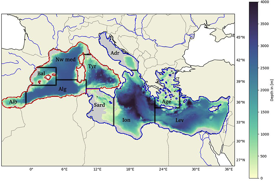
Figure 1. Bathymetric map of the Mediterranean Sea; gray areas represent the regions with depths less than 200 m. The red outline shows the Western Basin and the blue one the Eastern Basin. Alb, Alboran Sea; Bal, Balearic Sea; Alg, Algerian Sea; Nw Med, North-western Mediterranean Sea; Tyr, Tyrrhenian Sea; Sard, Sardinia Channel; Adr, Adriatic Sea; Ion, Ionian Sea; Lev, Levantine Sea; and Age, Aegean Sea.
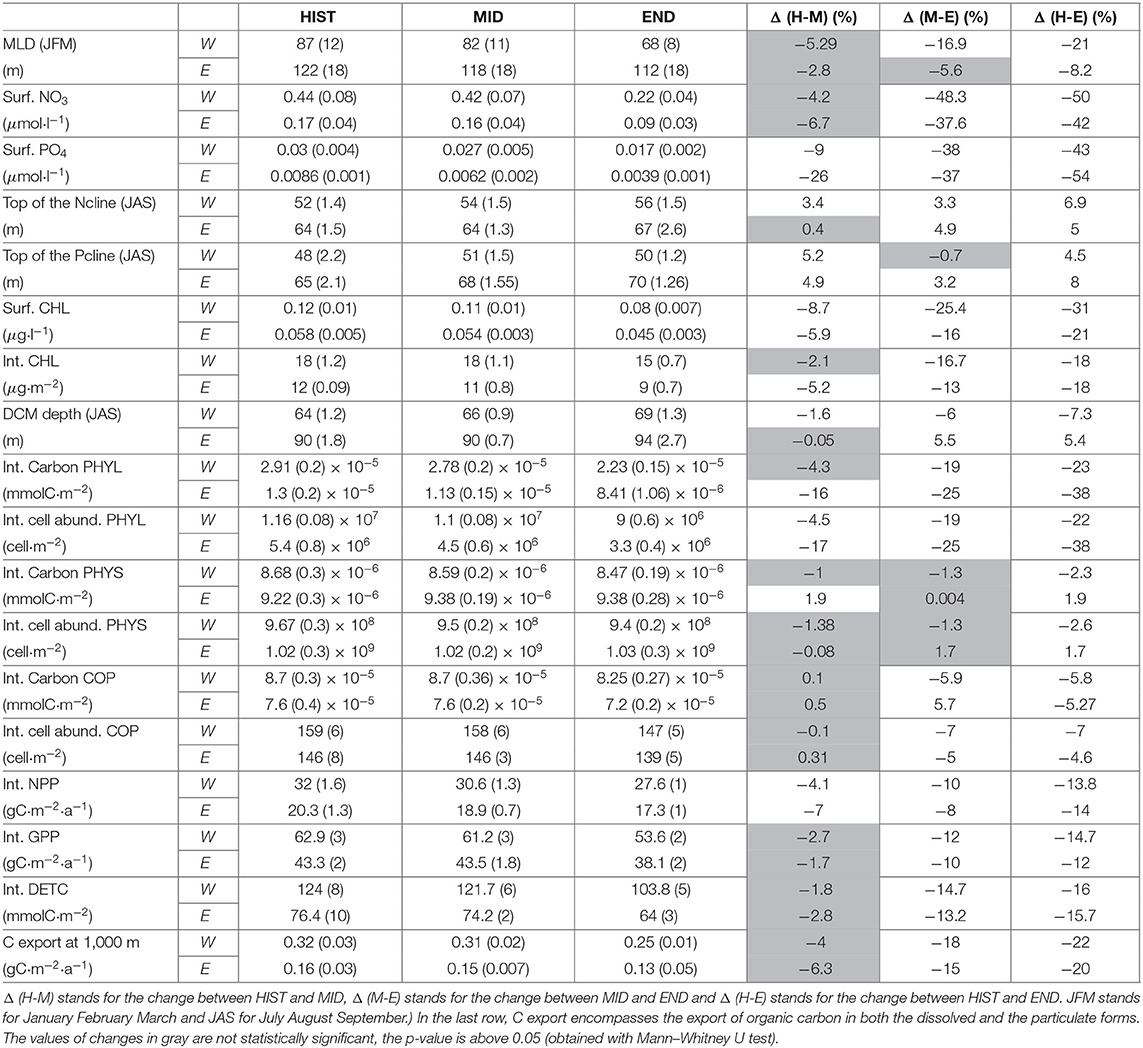
Table 1. Summary of the main values of the simulation, HIST refers to the 1986–2005 period, MID to the 2031–2050 period and END to 2081–2100 period.
Some variables, however, are averaged over specific seasons, to allow a more in-depth analysis. This is the case for the Mixed Layer Depth (MLD) which is an on-line and high-frequency diagnostic variable computed directly within the physical simulation (Darmaraki et al., 2019; Soto-Navarro et al., 2020). Starting from the surface, it corresponds to the first depth at which the potential density starts to differ from the density at 10 m by more than 0.011 kg m−3. In the present study, we focus on the winter maximum of the MLD instead of annual means. The winter maximum of MLD indeed directly constrains the amount of nutrients that will be brought to the surface layers during winter mixing, and therefore will sustain the biological production in the MED (Broecker and Peng, 1982; Williams, 2003; Van Den Broeck et al., 2004; Auger et al., 2014).
In the same way, the depth of the top nitracline (Ncline) and phosphocline (Pcline) are computed in summer (July to September) when stratification and depletion of nutrients in surface layers are the strongest. The top of the Ncline is defined as the first depth, starting from the surface, at which NO3 equals the threshold value of 0.05 μmol·l−1 which corresponds to the classical quantification limit of nitrate measurement using an autoanalyzer (Aminot and Kérouel, 2007). The top of the Pcline is based on the threshold value of 3 nmol·l−1 which is the threshold for the top of the Ncline divided by 16, namely the Redfield N:P ratio.
The DCM is also calculated during summer (July to September), i.e., when it is present in most of the MED. Finally, the Stratification Index (SI) is computed in summer (July to September) from the surface to a given depth using the Brunt-Vaisala frequency which is an indicator of the strength of the vertical stratification. The latter increases with the SI. It has been used in many Mediterranean studies (Lascaratos and Nittis, 1998; Herrmann et al., 2008; Somot et al., 2016).
In order to assess whether the changes between the HIST, MID, and END periods are significant, we applied a Mann-Whitney U test (a non-parametric version of the Student t-test). If the p-values are lower than 0.05, the variations are considered as statistically significant, and if the p-values are above 0.05, they are not (see the gray cells in Table 1).
3. Results
3.1. Model Skill Assessment
The biogeochemical model configuration (Eco3M-Med) is almost the same as the one used in Pagès et al. (2020) in which its capacity to successfully reproduce the main patterns of the biogeochemistry of the MS (i.e., surface CHL, nutrients distribution, primary production, etc.) has been demonstrated with a physical forcing at higher resolution (1/12° instead of 1/8°). For this reason, only an additional comparison is provided here (Figure 2). This figure shows the modeled (mCHL) and the observed (oCHL), i.e., satellite-derived, mean surface chlorophyll a concentration over the 1999–2006 period. In the Western Basin, both maps exhibit high chlorophyll concentration in the Gulf of Lions, along the Algerian coast and in the Alboran Sea. However, the modeled mean concentration (0.12 μg·l−1 over the Western Basin) is a little bit lower than the observed one (0.16 μg·l−1). Regarding the Eastern Basin, the model succeeds in representing the oligotrophic offshore area, but the mCHL is too low in several areas: (i) in the Gulf of Gabes where several factors may explain this discrepancy between model outputs and satellite data, for example the shallow depth of this area which may mean that the satellite-based data is polluted by the reflection from benthic vegetation (Jaquet et al., 1999). Another complementary explanation is that phosphate inputs in this industrial area are not taken into account by the model, though some recent work managed to simulate relatively high phytoplankton biomass in this region without additional phosphate inputs (Macias et al., 2019), (ii) in the vicinity of the Nile mouth where the nutrient inputs are very poorly known, as well as throughout the Western Adriatic Sea probably due to a lack of phosphate in the Pô River inputs, (iii) at the scale of the Eastern Basin, the mean values of mCHL and oCHL are respectively equal to 0.07 and 0.12 μg·l−1. However, if we exclude the coastal area (i.e., where the depth is <200 m) in order to avoid case II water (Bosc et al., 2004; Richon et al., 2018), the mean values of mCHL and oCHL are respectively equal to 0.055 and 0.06 μg·l−1. Furthermore, to rule out the assumption that the changes in the biogeochemistry cannot be ascribed to model drift, a control simulation has been run over the forecast period, namely from 2006 to 2100 (see section 2.4 for details). This control simulation did not exhibit any trend regarding the state variables, thereby enabling us to conclude that there is no drift inherent to the biogeochemical model.
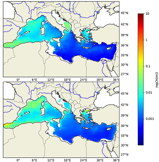
Figure 2. Average surface chlorophyll a concentration (excluding areas with depths <200 m) between 1999 and 2006, (top) calculated by the model and (bottom) observed by satellite (satellite data provided by CMEMS, more information in Barale and Gade, 2008).
On that basis, and accounting for the numerous previous comparisons with data performed for the historical period (Guyennon et al., 2015; Pagès et al., 2020), it is considered that the present model can be used to investigate the impact of climate change on the basin-scale biogeochemistry over the next century.
3.2. The Mixed Layer Depth
During the HIST period, the average winter MLD (Figure 3A) is deeper in the area of deep water formation (i.e., the Gulf of Lion, South Adriatic Sea, and the South Aegean Sea) and shallower in most of the other parts of the MED. Between the HIST and MID periods (Figure 3B) the winter MLD exhibits a slight decrease of almost 5.7% in the Western Basin (from 87 m for the HIST period to 82 m for the MID period) and of 2.8% in the Eastern Basin (from 122 m for the HIST period to 118 m for the MID period). However, those decreases are not statistically significant. Between the HIST and END periods, the winter MLD shows (Figure 3C) a substantial decrease of 21% in the Western Basin (from 87 m for the HIST period to 68 m for the END period) and of 8% in the Eastern Basin (from 122 m for the HIST period to 112 m for the END period). The Gulf of Lions region, and more generally the Western Basin, is the most affected, showing the strongest reduction in the maximum MLD, especially after 2050.
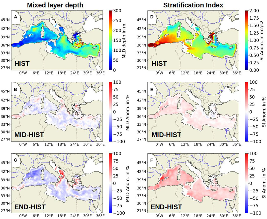
Figure 3. (A) Map of the winter Mixed Layer Depth (MLD) in m during the HIST period; (B) Map of the evolution of the modeled winter (January to March) MLD in percent between HIST and MID (the difference MID - HIST is plotted); (C) Map of the change in the modeled winter MLD in percent between HIST and END; (D) Map of the summer Stratification Index (SI) in m2· s −2 during the HIST period; (E) Map of the change of the modeled SI in percent between HIST and MID; (F) Map of the change of the modeled SI in percent between HIST and END.
Regarding the stratification index during the HIST period (Figure 3D), the area of deep water formation shows the weakest values. Furthermore, the Western Basin shows an SI stronger than the Eastern Basin with respectively 1.3 and 1 m2·s −2. The variation of SI between the HIST and MID periods (Figure 3E) shows an increase of 11% (from 1.3 for the HIST period to 1.45 m2·s −2 for the MID period) in the Western Basin and of 5% in the Eastern Basin (not statistically significant). Between HIST and END periods (Figure 3F) the increase is even more substantial with 29% (from 1.3 for the HIST period to 1.68 m2·s −2 for the END period) in the Western Basin and of 16% in the Eastern Basin (from 1 for the HIST period to 1.24 m2·s −2 for the END period). For SI as for the MLD, the Western Basin is more impacted than the Eastern Basin.
The variations between the three different periods mostly occur between the MID and the END periods, i.e., between 2050 and 2100. The details of variations between each period are given in Table 1. Further information on the variations in the MLD in the CNRM-8.5 simulation can be found in Soto-Navarro et al. (2020).
3.3. Scenario Results Associated With the Biogeochemistry of the MS
3.3.1. Nutrient Concentrations
The annual average surface concentration of NO3 and PO4 in the Western and Eastern Basins (Figure 4) do not show any clear trend up to the year 2050.
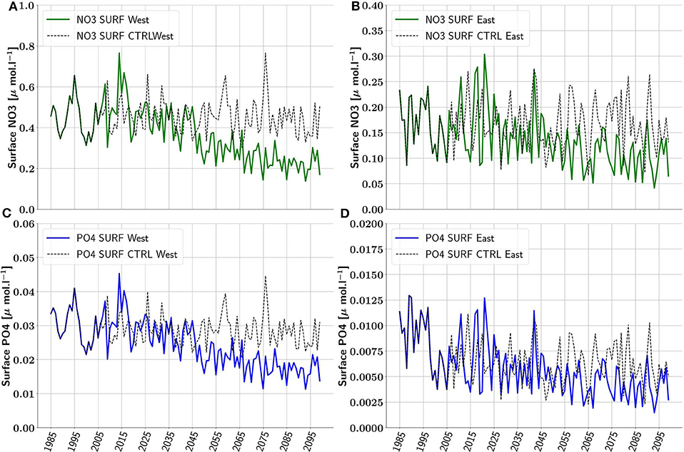
Figure 4. Annual average of surface concentrations of NO3 (green) and PO4 (blue) in (μmol·l−1) in the Western Basin (A,C) and the Eastern Basin (B,D). Black dotted line shows the control simulation.
After 2050 in the Western Basin, the surface NO3 concentration (Figure 4A) progressively declines from 0.42 μmol·l−1 in the MID period to 0.22 μmol·l−1 for the END period, corresponding to a decrease of 48.3% between MID and END (50% between HIST and END, Figure 5).
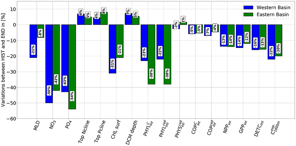
Figure 5. Changes (in percent) of the main biogeochemical variables calculated by the model between the HIST (1986–2005) and the END (2081–2100) periods.
For the surface PO4 concentrations in the Western Basin (Figure 4C) after 2050, we observe a decrease from 0.027 μmol·l−1 for the MID period to 0.017 μmol·l−1 for the END period. This represents a 38% decrease between MID and END (and a 43% decrease between HIST and END (Figure 5).
In the Eastern Basin, we observe the same trends for both NO3 and PO4 as for the Western Basin (Figures 4B,D). However, the decrease between the MID and the END periods is less than in the Western Basin and equal to 37.6% for NO3 and 37% for PO4. Between HIST and END the decrease reaches 42% for NO3 and 54% for PO4 (Figure 5).
Overall, the decline in nutrient concentrations is stronger in the Western Basin than in the Eastern Basin between MID and END. We can also observe that NO3 concentrations decrease more than those of PO4 between MID and END (respectively by 45% and by 37%) in the Western Basin, while in the Eastern Basin between MID and END the decrease is almost the same 37% for both nutrients. Between HIST and END, NO3 concentrations still decrease more than those of PO4 in the Western Basin (respectively by 50% and by 43%). But in the Eastern Basin, NO3 concentrations decrease less than those of PO4 (respectively by 42% and by 54%). All the values are available in Table 1.
The model also predicts a deepening of the top of the nitracline (Ncline) and the phosphocline (Pcline) after 2050 (Figure 5). The top of the Ncline remains constant in both basins until 2050, with an average depth of 53 and 64 m in the Western and Eastern Basins, respectively. Thenceforth, in 2050 Ncline starts to deepen to end up in the END period at 56 m in the Western Basin and 67 m in the Eastern Basin a deepening of respectively 6.9 and 5% between HIST and END (Figure 5). Regarding the Pcline, the same trends are shown by the model as for the Ncline, with an average depth of 51 m (68 m) for the Western (Eastern) Basin, for the MID period, and 50 m (70 m) for the END period, corresponding to a deepening of 0.7% (not statistically significant) in the Western Basin and to 3.2% in the Eastern Basin. Between HIST and END, the Pcline deepens of 4.5 and 8%, respectively in the Western and Eastern Basins.
3.3.2. Chlorophyll Concentration
The annual average of CHL exhibits a strong decline after 2050 in both basins. In the Western Basin (Supplementary Figure 1A), CHL quickly drops from 0.12 (0.11) μg·l−1 in the HIST (MID) periods down to 0.08 μg·l−1 in the END period, representing a decrease of ~31% (25.4%) (see Figure 5). In the Eastern Basin (Supplementary Figure 1B), CHL exhibits the same trends as in the Western Basin, the decrease is equal to 21% (16%) between HIST (MID) and END, CHL varies from 0.058 (0.054) to 0.045 μg·l−1. Looking at the depth of the Deep Chlorophyll Maximum (DCM) during summer (July to September) in the Western Basin (Supplementary Figure 1C), it can be observed that, the DCM deepens from 64 m (66 m) in the HIST (MID) period to 69 m in the END period, a deepening of 7.3% (6%) (see Figure 5). In the same way, in the Eastern Basin, no trend could be observed for the DCM between HIST and MID period, with an average DCM depth of 90 m. After 2050, the DCM deepens from 90 m in the MID period to 94 m in the END period, a deepening of 5.5% (Figure 5).
3.3.3. Phytoplankton Community
According to the model, the vertically-integrated cellular abundance of phytoplankton remains stable over the first half of the twenty-first century almost everywhere in the Mediterranean. After 2050, the vertically-integrated abundance of small phytoplankton () remains stable over both basins (changes are not statistically significant), as shown in Supplementary Figure 2 (left). The vertically-integrated cellular abundance of large phytoplankton () shown in Supplementary Figure 2 (right), decreases by 26% in the Western Basin and by 35% in the Eastern Basin between the MID and the END periods.
3.3.4. Primary Production Rates
In both basins, the annual vertically-integrated net primary production (NPPint) remains stable (Supplementary Figures 3A,B) between the HIST and the MID periods (variations are not statistically significant, p-value > 0.05). In the Western Basin, NPPint declines from 32 (30.6) gC·m−2·a−1 during the HIST (MID) period to 27.6 gC·m−2·a−1 at the END period, a reduction of 13.8% (10%) (see Figure 5). In the Eastern Basin, NPPint declines from 20.3 to 17.3 gC·m−2·a−1 between the HIST and the END periods (i.e., a reduction of 14%).
Regarding the annual vertically-integrated gross primary production (GPPint), it follows the same trend as NPPint but with higher values. In the Western Basin, GPPint declines from 62.9 gC·m−2·a−1 during the HIST period to 53.6 gC·m−2·a−1 for the END period (i.e., a reduction of 14.7%). In the Eastern Basin, NPPint declines from 43.3 to 38.1 gC·m−2·a−1 between the HIST and the END periods (i.e., a reduction of 12%).
3.3.5. Copepod Abundance and Biomass
The mean annual vertically-integrated carbon biomass () of copepods decreases in both basins after 2050 (Supplementary Figure 3, top). declines between the MID and END periods by 7% in the Western Basin and 6% in the Eastern Basin. Regarding the vertically-integrated abundance () of COP (Supplementary Figure 3, bottom), we observe a decline from 159 to 147 ind·m−2 between the MID and the END periods, representing a 8% decrease in the Western Basin. In the Eastern Basin, between MID and END, decreases from 147 to 139 ind·m−2, which corresponds to a decline of 5.4%.
3.3.6. Particulate and Dissolved Organic Carbon
The model also highlights changes (Figure 5) in Detrital Organic Carbon (DETC). In both basins, DETC integrated concentrations remain stable between HIST and MID (values are not statistically significant), with an average value of 123 and 75 mmolC·m−2, respectively for the Western Basin and the Eastern Basin. Then they strongly decline in both basins from 124 and 76.4 mmolC·m−2, respectively for the Western Basin and the Eastern Basin during HIST period to end up at 103.8 and 64 mmolC·m−2 at the END period, a decrease of 16% in both basins. Concerning the Dissolved Organic Carbon (DOC) the model did not exhibit any trend despite the slight increase in PHYS abundance (not shown).
3.3.7. Export of Organic Carbon
The annual average of particulate and dissolved organic carbon export at 1000 m () remains steady up to 2050 in both basins with average values of 0.32 gC·m−2·a−1 for the Western Basin (Supplementary Figure 5A) and 0.16 gC·m−2·a−1 for the Eastern Basin (Supplementary Figure 5B). After 2050, the starts to decline to end up at 0.25 gC·m−2·a−1 in the Western Basin and 0.13 gC·m−2·a−1 in the Eastern Basin, which corresponds to a decrease of respectively 20 and 22% between the HIST and the END periods, respectively (Figure 5).
3.3.8. Nutrients Availability After Winter Mixing
Figure 6 shows the mean nutrient profiles in autumn (September to November) and the position of the maximum MLD, averaged over the Western Basin, for the HIST, MID, and END periods. It should be noted that for better legibility, NO3 and PO4 concentrations in Figure 6 are shown on a different horizontal axis. The slope of the Ncline between its top and 100 m depth is weaker than the slope of the Pcline, and the annual maximum of MLD becomes shallower from HIST to END. Furthermore, the intersection between the deeper MLD and autumn nutrient profiles provides a rough estimation of the nutrient concentrations mixed with upper surface water. For the HIST period, winter mixing reaches a conceptual value of 3.42 (0.2) μmol·l−1 of NO3 (PO4). These values drop to 2.98 (0.17) and 1.11 (0.08) μmol·l−1 for NO3 (PO4), respectively during the MID and the END periods. This represents a 67% decrease in the NO3 concentrations induced by winter mixing between HIST and END, and a 60% decrease in PO4. In the Eastern Basin, the MLD variation (not shown) is statistically significant only between the HIST and the END periods. For the HIST period, winter mixing reaches a conceptual value of 2.59 (0.13) μmol·l−1 of NO3 (PO4). These values decrease to 1.66 (0.08) μmol·l−1 for NO3 (PO4), for the END period. This represents a 35% decrease between HIST and END in the NO3 concentration potentially reached by winter mixing, and a 38% decrease for that of PO4.
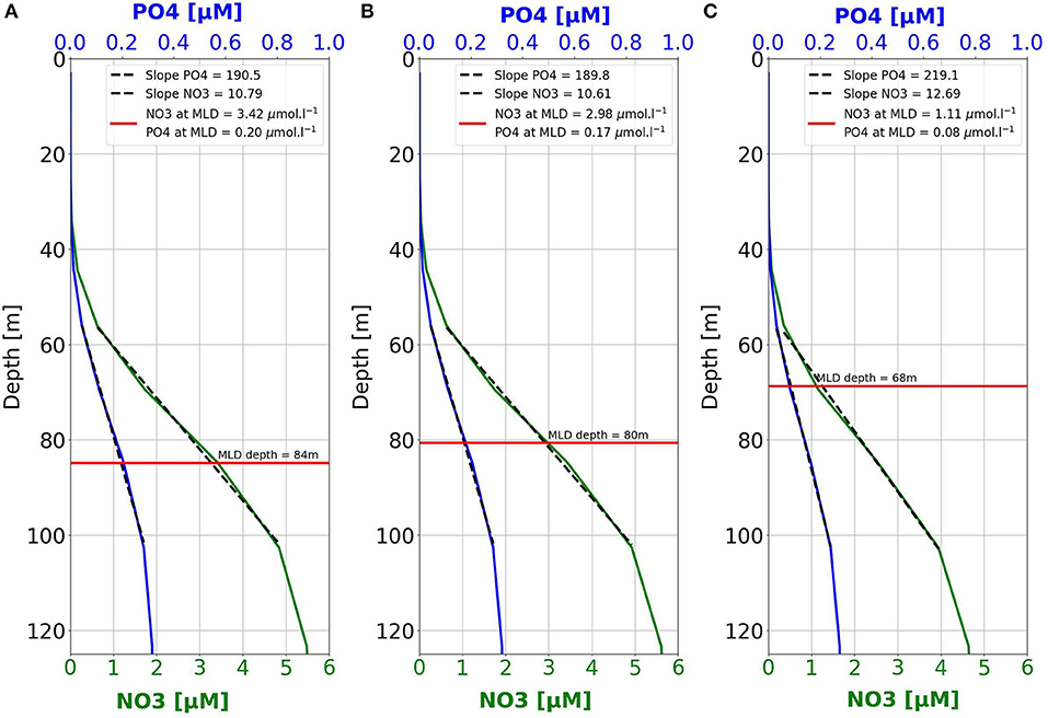
Figure 6. Average profiles in autumn (September to November) of NO3 (green) and PO4 (blue) for the Western Basin for the periods: (A) 1986–2005; (B) 2021–2050; (C) 2071–2100. The red line shows the average mixed layers depth (MLD) in winter (January to March) for the same periods. Dotted lines show the linear relationship between nutrient concentrations and depth (green NO3 and blue PO4) between 60 and 100 m. These depths have been arbitrarily chosen in order to best represent the gradient regions of the nutriclines.
3.3.9. Growth-Limiting Nutrients
The most limiting nutrient between 0 and 150 m among N and P during summer (which corresponds to the period where nutrients most limit phytoplankton growth) is shown for PHYS and PHYL in Figure 7. The most limiting nutrient X corresponds to the element for which QX (in mol X cell−1) is minimum, and is the mean normalized (i.e., comprised between 0 and 1) intracellular quota in element X. Furthermore, we consider that there is co-limitation when the difference between and does not exceed 5%. During the HIST period, PHYS (Figure 7A) is mainly limited by phosphorous (P) in the Western Basin (30% of its area) or co-limited by N and P (52% of its area). Nitrogen (N) limitation only occurs on 18% of the Western Basin area. During the END period, PHYS (Figure 7B) is mainly limited by N (42% of its area) or co-limited (41% of its area). P limitation only occurs on 17% of the Western Basin area. In the Eastern Basin during the HIST period, PHYS is mainly limited by P (75% of the area). N and N-P colimitation only occur on respectively 15 and 8% of the Eastern Basin area. During the END period, the limitation remains almost unchanged as compared to the situation during the HIST period.
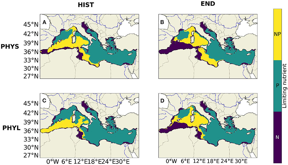
Figure 7. Map of the limiting nutrients over the 0–150 m layer during summer (July to September) for the 1986–2005 period (A,C) and the 2081–2100 period (B,D). (A,B) for PHYS and (C,D) for PHYL. The areas colored in purple are N limited, the green areas are P limited and the yellow areas are co-limited by N and P (meaning that the difference between N and P normalized cell quotas is <5%).
For PHYL (Figure 7C), during the HIST period, 46% of the area of the Western Basin is limited by P, 45% is co-limited and only 9% is limited by N. During the END period (Figure 7D), the limitation in N increases to reach 33% of the area of the Western Basin, the P limitation decreases down to 19%, and the co-limited area remains almost unchanged. In the Eastern Basin, for the HIST and the END periods, the limitation remains driven by phosphorus for more than 80% of its area.
4. Discussion
4.1. Relevance of the Present Scenario
This scenario explores the effects of the expected changes in hydrodynamics (according to the RCP 8.5 scenario) on the biogeochemistry of the MS. The other potential sources of variability of the biogeochemistry, namely the inputs of nutrients at the different boundaries (i.e., inputs of nutrients by rivers, at the Gibraltar Strait, or by atmospheric deposition) have deliberately not been considered at this stage. There are several reasons for this: (i) first, it is very informative to know the relative weight of each of the internal and external contributions to the future changes in the MS and one of the main strengths of modeling is precisely that it enables us to disentangle the role of each process and forcing. Aware of the potential role that could be played by river inputs throughout the MS, and not only near the river mouths (Macias et al., 2014; Moon et al., 2016; Pagès et al., 2020), we deliberately decided to maintain nutrient river outputs constant (the year 2000 is repeatedly used after 2000). This study has therefore enabled us to explore the changes ascribed to hydrodynamics alone, independently of the other sources of variability. It also provides a reference for future studies focused on the understanding of the role of nutrients boundary inputs on the biogeochemistry of the MS, (ii) unlike scenarios for hydrodynamics, the only available scenario for nutrient inputs by rivers provided by Ludwig et al. (2010) is very rudimentary since it provides two values (one for 2030 and another for 2050) for each of four scenarios of the Millenium Ecosystem Assessment. Such nutrients input scenarios are therefore liable to introduce a considerable additional uncertainty in the model outputs, all the more so as they are not consistent with the RCP 8.5 climate scenario used in the present study. Concerning atmospheric deposition, to our knowledge there is no transient scenario available so far describing the evolution of atmospheric deposition over the MS, (iii) by contrast, several coupled physical-biogeochemical simulations run at global scale and forced by the RCP 8.5 scenario are available. However, they provide very different (and even divergent) dynamics for nutrient concentrations in the next century. Moreover, some of them only provide the nutrients concentrations at the sea surface. In this context, and to consider the effects of hydrodynamics alone, the nutrients boundary concentrations at the Gibraltar Strait were kept constant (describing an annual climatology scenario). However, since the physical simulation used to force the biogeochemical model predicts an increase in the surface water inflow at Gibraltar straits of 0.03 Sv (Darmaraki et al., 2019), corresponding to an increase of 3.7% in the surface inflow over the next century (Soto-Navarro et al., 2020), this increase in the Gibraltar inflow implies an increase in the inflow of nutrients in the surface layer at the Gibraltar Strait and acts against nutrients decrease, and probably mitigates it in our simulation.
4.2. Analysis of the Scenario Results
The simulation shows a significant decrease in surface nutrients over the second half of the twenty-first century in the MS. Between the MID (2031–2050) and END (2081–2100) periods, the model shows a decrease of 48.3 and 37.6% of NO3 and 38 and 37% of PO4 (Figure 4) in the Western and the Eastern Basins, respectively. As already mentioned, these changes in nutrient concentrations and in the other state variables of the biogeochemical model can be ascribed to the effects of variations in hydrodynamics induced by climate change, independently of other sources of variability. Furthermore, considering that our model does not include the effect of temperature on the kinetics of the biogeochemical processes, and that currents are expected to remain almost unchanged (except locally in some areas), the main factor that could explain the decrease in nutrient concentrations is the vertical mixing and the associated MLD. The MLD is expected to progressively become shallower, mostly after 2050, as shown in Figure 3 and by Soto-Navarro et al. (2020). This decrease is directly linked to the increase of the stratification shown in Figure 3. The changes in water temperature and salinity over the next century induces a stronger stratification. Due to that stronger stratification of the water column, more energy is needed in winter to break it, and therefore, the winter mixed layer is shallower. This strong decrease in the winter MLD (nearly 20% in the Western Basin between HIST and END and 17% between MID and END), is probably responsible for the decline in surface nutrients after 2050 that mostly impacts the Western Basin (Figure 4). The decline in surface nutrients over the next century caused by an enhanced stratification has already been predicted in most global scale studies for the sub-tropical areas (Bopp et al., 2005, 2013; Marinov et al., 2010; Dutkiewicz et al., 2013, 2019; Bindoff et al., 2019). The same conclusion has been drawn for the MS by Lazzari et al. (2014) (SRES-A1B) or for the north-Western MS by Herrmann et al. (2014) (SRES-A2), though they both use discontinuous simulations and different climate scenarios. This conclusion is also that suggested by Macias et al. (2015) using a continuous simulation under RCP 8.5 climate condition and constant river inputs, but only for the Western Basin, whereas they predict an increase in nutrient concentrations in the Eastern Basin (due to the intensification of vertical mixing because of the increase in evaporation). This result is not in contradiction with our work since the nutrient decrease in the Eastern Basin is significantly weaker than that in the Western Basin. The study by Richon et al. (2019) obtained with a SRES-A2 scenario indicates that nitrate will be accumulating in the surface layers of the MS over the twenty-first century, while there is no trend in surface phosphate concentrations. However, according to these authors, this is the result of the effects of river and Gibraltar inputs since the reduction of vertical mixing makes surface water more sensitive to external nutrient inputs.
The decrease in nutrient concentrations in the surface layer is concomitant with the deepening of the top of the Ncline and the top of the Pcline, as shown by the model in both basins in summer [the depth of the top of the Ncline increases by 6.9% (5%) and that of the Pcline by 4.5% (8%) in the Western Basin (Eastern Basin)]. The deepening of nutriclines results in less nutrients being brought to the surface layer during winter, which results in the oligotrophication of the surface layer. In the model, the top of the nutriclines under stratified conditions is driven by the equilibrium between the production flux (mineralization through bacterial activity), and the consumption flux of nutrients. Those processes are extensively explained in Pagès et al. (2020). Since nutrient quantities brought to the upper layer during vertical mixing progressively decrease, phytoplankton has to go deeper to find available nutrients in summer to sustain its growth and it progressively erodes the top of the nutriclines. The deepening of phytoplankton during summer is indeed predicted by our simulation through the deepening of the DCM (Supplementary Figures 1C,D). The depth of the DCM increases by 7.3% in the Western Basin and by 5.4% in the Eastern Basin, following the same trend as nutricline depths. A slight deepening of the DCM has already been shown at regional scale by Richon et al. (2019), but Macias et al. (2015) predict a small reduction of the mean depth of the DCMs (mean reduction of 1.2 m over the MS).
Another effect of nutrient decline in the surface layer is the reduction of the surface CHL concentration after 2050 (Supplementary Figure 1). Our simulation do indeed predict a 31% decrease in surface CHL in the Western Basin and 21% in the Eastern Basin between HIST and END, however most of this decrease occurs between MID and END with a reduction of 25% for the Western Basin and of 16% for the Eastern Basin. This is in accordance with the study of Dutkiewicz et al. (2019) at global scale which shows a reduction of CHL in several regions of the ocean after 2030 (0.5% a−1 for the North Atlantic). Richon et al. (2019) also highlighted an almost 9% decline in the integrated CHL over the MS (while this study shows a 16% decline in the vertically-integrated CHL in the Western Basin and of 3.4% in the Eastern Basin). Finally, the study by Herrmann et al. (2014) shows an opposite trend with a 8% increase in the integrated CHL over the north-western MS. However, primary production is positively correlated with temperature in their model through an exponential law (Eppley, 1972), which increases the photosynthesis rate as temperature increases.
The aforementioned drop in surface CHL concentrations is related to the reduction of PHYL abundance () (Supplementary Figure 2) and carbon biomass () simulated mostly after 2050 (not shown), as a consequence of the increasing oligotrophy. By contrast, PHYS which is better adapted to oligotrophic conditions, slightly increases in the Eastern Basin, but not enough to compensate the lack of CHL due to PHYL decline (PHYL is indeed responsible for a large part of the CHL production, mostly during the spring bloom period). The study by Flombaum et al. (2013) also predicts at global scale, that small phytoplankton (Prochlorococcus and Synechococcus) abundance will be enhanced (respectively by 29 and 14%) in the next century. Our study is also in agreement with the study of Herrmann et al. (2014) who showed that the planktonic community structure should evolve toward larger biomasses of small-size groups [picophytoplankton (+25%), bacteria (+18%) and nanozooplankton (+17%)]. Richon et al. (2019) showed that diatoms were expected to be more sensitive to climate change as their simulated biomass decreased more sharply than that of nanophytoplankton. Overall, it has been shown by most studies at global scale that large phytoplankton are more disadvantaged when external conditions become more nutrient-depleted (Bopp et al., 2005; Marinov et al., 2010; Dutkiewicz et al., 2013).
As a result of the drop in and in surface and DCM CHL (Supplementary Figure 1), the integrated primary-production decreases by 12.7 and 14%, respectively for NPPint and GPPint in the Western Basin and by 9.3 and 11%, respectively for NPPint and GPPint in the Eastern Basin between MID and END periods. The historical value of GPPint, namely 63 and 43 gC·m−2·a−1, respectively for the Western and the Eastern basins are in good agreement with the literature, although at the lower end of the range. For example if we focus on modeling studies, Guyennon et al. (2015) calculate a GPP of 82 gC·m−2·a−1 for the whole Mediterranean basin, while Lazzari et al. (2012) obtain an average of 98 gC·m−2·a−1 and Crispi et al. (2002) of 88 gC·m−2·a−1. The satellite values are more sparse from 68 gC·m−2·a−1 (Uitz et al., 2012) to 136 gC·m−2·a−1 (Bosc et al., 2004). Regarding in situ values, Siokou-Frangou et al. (2010) show ranges between 59 and 150 gC·m−2·a−1 and according to Ryther (1969), oligotrophy is characterized by a primary production smaller than 50 gC·m−2·a−1.
Most of the climate scenarios at global scale suggest a decrease in NPP, though in some specific regions, an increase has been predicted (Bopp et al., 2005, 2013; Dutkiewicz et al., 2013, 2019; Yool et al., 2013). Bopp et al. (2013) and Yool et al. (2013) have predicted a 8.6 and 6.3% reduction of the NPPint at global scale by the end of the century, respectively. Finally, Bindoff et al. (2019) show that tropical NPP will decline by 7–16% by 2100. At a regional scale, the conclusions of previous studies are more sparse. Lazzari et al. (2014) did not predict any trend in the NPP (but with a discontinuous scenario only spanning the 1990–2000 and 2090–2100 periods), Macias et al. (2015) pointed out a decrease of the primary production rate in the Western Basin and an increase in the Eastern Basin. Richon et al. (2019) show a 10% reduction of the NPPint. Finally, some studies also predict an increase in primary production, with Herrmann et al. (2014) showing a 19% increase in the Gross Primary Production (GPP) for the north-western MS and Moullec et al. (2019) reporting an increase in the NPP stronger in the Eastern Basin than in the Western Basin.
The decline in and also directly impacts its main predator in the model, namely the mesozooplankton (Supplementary Figure 4). Our model shows that () decreases by 7% in the Western Basin and 5% in the Eastern Basin. This result is consistent with the fact that large organisms are disadvantaged in oligotrophic areas. In addition, Stock et al. (2014) show a 7.9% reduction of mesozooplankton using a RCP 8.5 scenario. In our model, the fact that decreases, may have potentially significant effects on small pelagic fishes such as sardines and anchovy, as pointed out by Woodworth-Jefcoats et al. (2017) for the tropical regions and suggested in Pagès et al. (2020) for the MS.
The decrease in and also induces a 16% (14.7%) and 15.6% (13.2%) reduction of DETCint in the Western Basin and Eastern Basin, respectively between HIST and END (MID and END). In the model, the DETC compartment is only fueled by PHYL and COP through the processes of mortality or fecal pellets production. The simulated dissolved organic carbon (DOC) did not exhibit any trend despite the increase in . The decrease in DETCint directly affects the export of organic matter at 1000 m (), which decreases by 22% (18%) and 20% (15%) in the Western Basin and the Eastern Basin, respectively (Supplementary Figure 5) between HIST and END (MID and END). At global scale, Bopp et al. (2001) show a 6% reduction of carbon export at 100 m, while Dutkiewicz et al. (2013) show a 10% decrease in organic export below 100 m. Bopp et al. (2013) also highlight a decrease in carbon export at 100 m at global scale due to reduced primary production combined with a change in the plankton community in favor of small organisms. Recently, it has been shown for the global ocean by Bindoff et al. (2019) that the downward carbon flux at 1000 m should decrease by 9 to 16% by 2100 under a RCP 8.5 scenario. At regional scale however, Herrmann et al. (2014) and Moullec et al. (2019) show that the organic export remains stable or even increases.
4.3. The Strong Decrease in NO3 Concentration in the Western Basin and Its Effect on Plankton Community
In the previous section, we highlighted that nutrient concentrations in the surface layers are expected to decline in both basins. However, in the Western Basin, the drop is higher for NO3 (50%) than PO4 (43%). By contrast, in the Eastern Basin, the decrease in PO4 (54%) is stronger than the decline in NO3 (42%) between HIST and END. Since the MLD is, in the present simulation, the main factor underlying the predicted trends in nutrient concentrations (see section 4.2), we can consider that the maximum depth of the MLD reached during winter drives the quantity of nutrients that will be available in the surface layer to sustain the biological production for the rest of the year. This quantity of nutrients is also strongly linked to the shape of nutrients vertical profiles in the water column. When looking at the profiles shape for the HIST, MID and END periods in the Western Basin (Figure 6), the slope of NO3 profiles is weaker than that of PO4, which means that NO3 concentrations decline more rapidly with depth. For the HIST period, the average of the maximum MLD values is 84 m (see section 3 and Table 1), corresponding to values of 3.42 and 0.2 μmol·l−1, for NO3 and PO4, respectively, that can be achieved by the vertical mixing. During the MID period, the values drop, respectively to 2.98 and 0.17 μmol·l−1 for NO3 and PO4, which means a decrease of 20% for both nutrients. For the END period, the values are now equal to 1.11 (0.08) μmol·l−1 for NO3 (PO4), corresponding to a 62.7% (52.9%) decline between MID and END periods. In other words, the slight difference in the shapes of the Ncline and the Pcline that arose between the MID and the END periods led to a 9% deficit in NO3 inputs by winter vertical mixing as compared to those of PO4. This provides a possible explanation for the stronger deepening of the Ncline (5.3%) than the Pcline (2%) in the Western Basin shown by the model. Since 2050, the NO3:PO4 ratio at the winter MLD depth regularly decreases (not shown). This leads to a drop in the N:P ratio in DET and DOM (not shown) in the upper layer of the Western Basin. Due to that decrease, the available amount of N for mineralization is lower than the amount of P at depth. This implies a stronger deepening of the Ncline than the Pcline in the Western Basin which progressively increases the shift between the NO3 and PO4 surface concentrations.
If we focus now on the Eastern Basin (not shown), between HIST and END the decrease of nutrients concentration at the MLD depth reaches quite similar values for NO3 and PO4, namely 35 and 38%. Those similar values are due to the MLD being deeper in the Eastern Basin than in the Western Basin and to the fact that both nutriclines at this depth are steeper and their slopes are closer.
To explain the 12% gap in the surface layer between PO4 and NO3, we need to focus on the rivers' nutrient inputs. In the simulation, in the Eastern Basin, PO4 inputs strongly decrease between 1985 and 2000 (Ludwig et al., 2009). This induces a progressive deepening of the phosphocline (while the nitracline remains at the same depth) in the Eastern Basin, as shown in a previous paper (Pagès et al., 2020). Due to that deepening of the phosphocline the amount of PO4 brought to the surface by winter vertical mixing decreases. That leads to a strong PO4 reduction in the surface layer lasting in the model at least until 2010 despite the fact that rivers nutrients inputs after the year 2000 are set constant in this simulation. This reduction in rivers' nutrient inputs could explain why the Eastern Basin shows a stronger decrease in PO4 than in NO3 between HIST and END. For the Western Basin, the changes in rivers' nutrient inputs during the 1985–2000 period are far less significant and do not impact the nutriclines depth (Pagès et al., 2020).
Since NO3 concentration declines more than that of PO4 in the surface layer of the Western Basin, changes in factors controlling plankton growth during summer occur. A significant part of the 0–150 m depth area where PHYS growth was mostly limited by P, progressively becomes limited by N or co-limited by N and P in the Western Basin (Figure 7). We observe a shift from a 30% P-limited and 18% N-limited in the Western Basin for the HIST period, to a 17% P-limited and 42% N-limited in the Western Basin by the end of the century. By contrast, there is no significant change in limiting nutrients in the Eastern Basin since NO3 and PO4 decline in a similar way in this basin.
For PHYL, we observe the same trend as for PHYS toward an expansion of the N-limitation in the Western Basin.
5. Conclusions
This study offers new insights regarding the possible effects of variations in hydrodynamic forcing induced by climate change on the biogeochemistry of the Mediterranean Sea and enhances the findings of other studies. It is the first RCP 8.5 continuous scenario run for the MS between 1985 and 2100 with a fully flexible-stoichiometry model, here the Eco3M-MED model having the distinctive characteristics of considering the abundance of the different PFTs and not directly taking into account the temperature effects on the biogeochemical processes. Moreover, the physical forcing used here is innovative because it is derived from a coupled model (CNRM-RCSM4) with a high degree of consistency between oceanic and atmospheric forcing.
This study highlights that most of the changes in the biogeochemistry of the MS could occur (under the RCP 8.5 scenario) after 2050. Before that, the changes remain sparse for most variables. The model clearly shows a strong decline in surface nutrients throughout the MS, which is in good accordance with regional and global studies. To our knowledge, this study is the first to show a discrepancy between the respective decrease of NO3 and of PO4 surface concentrations in the Western Basin after 2050 and to provide an explanation for it: because the slope of the average autumn NO3 profile is flatter than the slope of the average autumn PO4 profile, when the MLD becomes deeper during winter the amount of NO3 brought into the upper layers by vertical mixing is weaker than the amount of PO4. This discrepancy induces significant changes in the Western Basin, such as a deepening of the Ncline under the Pcline as well as significant changes in the limiting nutrients for phytoplankton and bacteria.
We also show in this work a strong decline in surface CHL concentrations (as well as at the DCM depth), in integrated net primary production and in biomass and abundance of large organisms (PHYL and COP) that could have a strong impact on the small pelagic fish community.
We also pointed out a strong decrease in organic carbon exports at 1000 m in both basins mostly due to the reduction of the abundance and biomass of PHYL and COP. We show in addition that variations in hydrodynamic forcing induced by climate change alone under the RCP 8.5 emission scenario will lead to a strong increase in the oligotrophy of the MS, and that the Western Basin seems to be more impacted than the Eastern Basin.
Finally, our study shows that the projected effects of climate-induced changes in hydrodynamics on the biogeochemistry of the Mediterranean Sea under a RCP 8.5 regional climate scenario are far from negligible.
As such, this scenario was highly instructive and has enabled us to disentangle the effects of hydrodynamics alone. These changes could be even more important if nutrient inputs by rivers and at the Gibraltar Strait were to decrease, or mitigated if they were to increase. The relative contributions of each of the internal and external sources of variability should be calculated in the future when all the forcing scenarios would be available.
Further work is necessary to provide a consistent prediction of the biogeochemistry of the MS by the end of the century. This study is indeed intended to be a first step toward an integrated prediction of land and sea responses to global change in the Mediterranean Basin using an integrated process-based model which will allow the use of consistent inputs of nutrients by rivers.
To conclude, this work and the forthcoming one will not be enough to explore all the different sources of uncertainties that could impact future projections (choice of scenarios, choice of models, internal variability, external nutrients inputs) and for this purpose, coordinated studies should be carried out in the future, as already done for physical projections.
Data Availability Statement
The raw data supporting the conclusions of this article will be made available by the authors on request.
Author Contributions
All authors listed have made a substantial, direct and intellectual contribution to the work, and approved it for publication.
Funding
This study has been made possible thanks to a Ph.D. thesis funded by the LaSeR-Med project. This project was part of the Labex OT-Med (no. ANR-11-LABX-0061) funded by the French Government Investissements d'Avenir program of the French National Research Agency (ANR) through the A*MIDEX project (no ANR-11-IDEX-0001-02). This work was performed using HPC resources from GENCI-IDRIS (Grant 2018-0227). This work was also a contribution to the MISTRALS/MerMex program. The physical simulation performed with CNRM-RCSM4 has been carried out on the Meteo-France computing facilities. It was a contribution to the Med-CORDEX multi-model initiative (Ruti et al., 2016) and can be downloaded from the Med-CORDEX database (www.medcordex.eu).
Conflict of Interest
The authors declare that the research was conducted in the absence of any commercial or financial relationships that could be construed as a potential conflict of interest.
Supplementary Material
The Supplementary Material for this article can be found online at: https://www.frontiersin.org/articles/10.3389/fmars.2020.563615/full#supplementary-material
Supplementary Figure 1. Annual average of surface chlorophyll concentration μg.l−1 (blue line on the top) for the Western Basin (A) and the Eastern Basin (B). The black dotted line shows the control simulation. The summer (July to September) average of the deep chlorophyll maximum depth (green) and of the chlorophyll concentration at the Deep Chlorophyll Maximum depth (red) are also plotted for the Western Basin (C) and the Eastern Basin (D).
Supplementary Figure 2. Map of the percentage of changes of the average vertically-integrated (surface to bottom) abundance (left for PHYS and right for PHYL) between the MID period (2031–2050) and the END period (2081–2100).
Supplementary Figure 3. Vertically-integrated net primary production averaged over the Western Basin (A) and the Eastern Basin (B) and vertically-integrated gross primary production averaged over the Western Basin (C) and the Eastern Basin (D) in gC·m−2·a−1. The black dotted line shows the control simulation.
Supplementary Figure 4. Annual mean of the vertically-integrated (surface to bottom) biomass in mmolC·m−2 (green) and abundance in cell·m−2 (blue) of Copepods averaged over the Western Basin (A,C) and the Eastern Basin (B,D). The black dotted line shows the control simulation.
Supplementary Figure 5. Annual mean of particular and dissolved organic carbon export in gC·m−2·a−1 at 1000 m averaged over the Western Basin (A) and the Eastern Basin (B). The black dotted line shows the control simulation.
References
Adloff, F., Somot, S., Sevault, F., Jordà, G., Aznar, R., Déqué, M., et al. (2015). Mediterranean Sea response to climate change in an ensemble of twenty first century scenarios. Clim. Dyn. 45, 2775–2802. doi: 10.1007/s00382-015-2507-3
Alekseenko, E., Raybaud, V., Espinasse, B., Carlotti, F., Queguiner, B., Thouvenin, B., et al. (2014). Seasonal dynamics and stoichiometry of the planktonic community in the NW Mediterranean Sea: a 3D modeling approach. Ocean Dyn. 64, 179–207. doi: 10.1007/s10236-013-0669-2
Allen, M., Dube, O., Solecki, W., Aragon-Durand, F., Cramer, W., Humphreys, S., et al. (2018). Global Warming of 1.5°C. An IPCC Special Report on the Impacts of Global Warming of 1.5° Above Pre-industrial Levels and Related Global Greenhouse Gas Emission Pathways, in the Context of Strengthening the Global Response to the Threat of Climate Change.
Aminot, A., and Kérouel, R. (2007). Dosage Automatique des Nutriments dans les Eaux Marines: Méthodes en Flux Continu.
Auger, P., Ulses, C., Estournel, C., Stemmann, L., Somot, S., and Diaz, F. (2014). Interannual control of plankton communities by deep winter mixing and prey/predator interactions in the NW Mediterranean: results from a 30-year 3D modeling study. Prog. Oceanogr. 124, 12–27. doi: 10.1016/j.pocean.2014.04.004
Baklouti, M., Diaz, F., Pinazo, C., Faure, V., and Quéguiner, B. (2006a). Investigation of mechanistic formulations depicting phytoplankton dynamics for models of marine pelagic ecosystems and description of a new model. Prog. Oceanogr. 71, 1–33. doi: 10.1016/j.pocean.2006.05.002
Baklouti, M., Faure, V., Pawlowski, L., and Sciandra, A. (2006b). Investigation and sensitivity analysis of a mechanistic phytoplankton model implemented in a new modular numerical tool (Eco3M) dedicated to biogeochemical modelling. Prog. Oceanogr. 71, 34–58. doi: 10.1016/j.pocean.2006.05.003
Barale, V., and Gade, M. (2008). Remote Sensing of the European Seas. Dordrecht: Springer Netherlands.
Beuvier, J., Sevault, F., Herrmann, M., Kontoyiannis, H., Ludwig, W., Rixen, M., et al. (2010). Modeling the Mediterranean Sea interannual variability during 1961–2000: focus on the Eastern Mediterranean transient. J. Geophys. Res. 115:C08017. doi: 10.1029/2009JC005950
Bindoff, N. L., Cheung, W. W. L., and Kairo, J. G. (2019). Changing Oean, Marine Ecosystems, and Dependent Communities. Special Report: The Ocean and Cryosphere in a Changing Climate Summary for Policymakers.
Bopp, L., Aumont, O., Cadule, P., Alvain, S., and Gehlen, M. (2005). Response of diatoms distribution to global warming and potential implications: a global model study. Geophys. Res. Lett. 32, 1–4. doi: 10.1029/2005GL023653
Bopp, L., Monfray, P., Aumont, O., Dufresne, J. L., Le Treut, H., Madec, G., et al. (2001). Potential impact of climate change on marine export production. Glob. Biogeochem. Cycles 15, 81–99. doi: 10.1029/1999GB001256
Bopp, L., Resplandy, L., Orr, J. C., Doney, S. C., Dunne, J. P., Gehlen, M., et al. (2013). Multiple stressors of ocean ecosystems in the 21st century: projections with CMIP5 models. Biogeosciences 10, 6225–6245. doi: 10.5194/bg-10-6225-2013
Bosc, E., Bricaud, A., and Antoine, D. (2004). Seasonal and interannual variability in algal biomass and primary production in the Mediterranean Sea, as derived from 4 years of SeaWiFS observations. Glob. Biogeochem. Cycles 18:GB1005. doi: 10.1029/2003GB002034
Colin, J., Déqué, M., Radu, R., and Somot, S. (2010). Sensitivity study of heavy precipitation in limited area model climate simulations: influence of the size of the domain and the use of the spectral nudging technique. Tellus A 62, 591–604. doi: 10.1111/j.1600-0870.2010.00467.x
Cramer, W., Guiot, J., Fader, M., Garrabou, J., Gattuso, J.-P., Iglesias, A., et al. (2018). Climate change and interconnected risks to sustainable development in the Mediterranean. Nat. Clim. Change 8, 972–980. doi: 10.1038/s41558-018-0299-2
Crispi, G., Crise, A., and Solidoro, C. (2002). Coupled Mediterranean ecomodel of the phosphorus and nitrogen cycles. J. Mar. Syst. 33–34, 497–521. doi: 10.1016/S0924-7963(02)00073-8
Darmaraki, S., Somot, S., Sevault, F., Nabat, P., Cabos Narvaez, W. D., Cavicchia, L., et al. (2019). Future evolution of marine heatwaves in the Mediterranean Sea. Clim. Dyn. 53, 1371–1392. doi: 10.1007/s00382-019-04661-z
Decharme, B., Alkama, R., Douville, H., Becker, M., and Cazenave, A. (2010). Global evaluation of the ISBA-TRIP continental hydrological system. Part II: uncertainties in river routing simulation related to flow velocity and groundwater storage. J. Hydrometeorol. 11, 601–617. doi: 10.1175/2010JHM1212.1
Dlugokencky, E., and Tans, P. (2019). Trends in Atmospheric Carbon Dioxide. National Oceanic & Atmospheric Administration, EarthSystem Research Laboratory.
Durrieu de Madron, X., Guieu, C., Sempéré, R., Conan, P., Cossa, D., D'Ortenzio, F., et al. (2011). Marine ecosystems' responses to climatic and anthropogenic forcings in the Mediterranean. Prog. Oceanogr. 91, 97–166. doi: 10.1016/j.pocean.2011.02.003
Dutkiewicz, S., Hickman, A. E., Jahn, O., Henson, S., Beaulieu, C., and Monier, E. (2019). Ocean colour signature of climate change. Nat. Commun. 10:578. doi: 10.1038/s41467-019-08457-x
Dutkiewicz, S., Scott, J. R., and Follows, M. J. (2013). Winners and losers: ecological and biogeochemical changes in a warming ocean. Glob. Biogeochem. Cycles 27, 463–477. doi: 10.1002/gbc.20042
Flombaum, P., Gallegos, J. L., Gordillo, R. A., Rincón, J., Zabala, L. L., Jiao, N., et al. (2013). Present and future global distributions of the marine Cyanobacteria Prochlorococcus and Synechococcus. Proc. Natl. Acad. Sci. U.S.A. 110, 9824–9829. doi: 10.1073/pnas.1307701110
Giorgi, F. (2006). Climate change hot-spots. Geophys. Res. Lett. 33:L08707. doi: 10.1029/2006GL025734
Guyennon, A., Baklouti, M., Diaz, F., Palmieri, J., Beuvier, J., Lebaupin-Brossier, C., et al. (2015). New insights into the organic carbon export in the Mediterranean Sea from 3-D modeling. Biogeosciences 12, 7025–7046. doi: 10.5194/bg-12-7025-2015
Herrmann, M., Estournel, C., Adloff, F., and Diaz, F. (2014). Impact of climate change on the northwestern Mediterranean Sea pelagic planktonic ecosystemand associated carbon cycle. J. Geophys. Res. Oceans 119, 1–22. doi: 10.1002/2014JC010016
Herrmann, M., Somot, S., Calmanti, S., Dubois, C., and Sevault, F. (2011). Representation of spatial and temporal variability of daily wind speed and of intense wind events over the Mediterranean Sea using dynamical downscaling: impact of the regional climate model configuration. Nat. Hazards Earth Syst. Sci. 11, 1983–2001. doi: 10.5194/nhess-11-1983-2011
Herrmann, M., Somot, S., Sevault, F., Estournel, C., and Déqué, M. (2008). Modeling the deep convection in the northwestern Mediterranean Sea using an eddy-permitting and an eddy-resolving model: case study of winter 1986–1987. J. Geophys. Res. 113:C04011. doi: 10.1029/2006JC003991
Houpert, L., Testor, P., Durrieu de Madron, X., Somot, S., D'Ortenzio, F., Estournel, C., et al. (2015). Seasonal cycle of the mixed layer, the seasonal thermocline and the upper-ocean heat storage rate in the Mediterranean Sea derived from observations. Prog. Oceanogr. 132, 333–352. doi: 10.1016/j.pocean.2014.11.004
Jaquet, J.-M., Tassan, S., Barale, V., and Sarbaji, M. (1999). Bathymetric and bottom effects on CZCS chlorophyll-like pigment estimation: data from the Kerkennah Shelf (Tunisia). Int. J. Rem. Sens. 20, 1343–1362. doi: 10.1080/014311699212777
Lascaratos, A., and Nittis, K. (1998). A high-resolution three-dimensional numerical study of intermediate water formation in the Levantine Sea. J. Geophys. Res. Oceans 103, 18497–18511. doi: 10.1029/98JC01196
Lazzari, P., Mattia, G., Solidoro, C., Salon, S., Crise, A., Zavatarelli, M., et al. (2014). The impacts of climate change and environmental management policies on the trophic regimes in the Mediterranean Sea: scenario analyses. J. Mar. Syst. 135, 137–149. doi: 10.1016/j.jmarsys.2013.06.005
Lazzari, P., Solidoro, C., Ibello, V., Salon, S., Teruzzi, A., Béranger, K., et al. (2012). Seasonal and inter-annual variability of plankton chlorophyll and primary production in the Mediterranean Sea: a modelling approach. Biogeosciences 9, 217–233. doi: 10.5194/bg-9-217-2012
Leblanc, K., Arístegui, J., Armand, L., Assmy, P., Beker, B., Bode, A., et al. (2012). A global diatom database–abundance, biovolume and biomass in the world ocean. Earth Syst. Sci. Data 4, 149–165. doi: 10.5194/essd-4-149-2012
Levy, H., Horowitz, L. W., Schwarzkopf, M. D., Ming, Y., Golaz, J.-C., Naik, V., et al. (2013). The roles of aerosol direct and indirect effects in past and future climate change. J. Geophys. Res. Atmos. 118, 4521–4532. doi: 10.1002/jgrd.50192
Lionello, P., Malanotte-Rizzoli, P., Boscolo, R., Alpert, P., Artale, V., Li, L., et al. (2006). The Mediterranean climate: an overview of the main characteristics and issues. Dev. Earth Environ. Sci. 4, 1–26. doi: 10.1016/S1571-9197(06)80003-0
Ludwig, W., Bouwman, A. F., Dumont, E., and Lespinas, F. (2010). Water and nutrient fluxes from major Mediterranean and Black Sea rivers: past and future trends and their implications for the basin-scale budgets. Glob. Biogeochem. Cycles 24:GB0A13. doi: 10.1029/2009GB003594
Ludwig, W., Dumont, E., Meybeck, M., and Heussner, S. (2009). River discharges of water and nutrients to the Mediterranean and Black Sea: major drivers for ecosystem changes during past and future decades? Prog. Oceanogr. 80, 199–217. doi: 10.1016/j.pocean.2009.02.001
Macias, D., Garcia-gorriz, E., Piroddi, C., and Stips, A. (2014). Biogeochemical control of marine productivity in the Mediterranean Sea during the last 50 years. Glob. Biogeochem. Cycles 28, 897–907. doi: 10.1002/2014GB004846
Macias, D., Huertas, I. E., Garcia-Gorriz, E., and Stips, A. (2019). Non-Redfieldian dynamics driven by phytoplankton phosphate frugality explain nutrient and chlorophyll patterns in model simulations for the Mediterranean Sea. Prog. Oceanogr. 173, 37–50. doi: 10.1016/j.pocean.2019.02.005
Macias, D. M., Garcia-Gorriz, E., and Stips, A. (2015). Productivity changes in the Mediterranean Sea for the twenty-first century in response to changes in the regional atmospheric forcing. Front. Mar. Sci. 2:79. doi: 10.3389/fmars.2015.00079
Marinov, I., Doney, S. C., and Lima, I. D. (2010). Response of ocean phytoplankton community structure to climate change over the 21st century: partitioning the effects of nutrients, temperature and light. Biogeosciences 7, 3941–3959. doi: 10.5194/bg-7-3941-2010
Mauriac, R., Moutin, T., and Baklouti, M. (2011). Accumulation of DOC in low phosphate low chlorophyll (LPLC) area: is it related to higher production under high N:P ratio? Biogeosciences 8, 933–950. doi: 10.5194/bg-8-933-2011
Moon, J.-Y., Lee, K., Tanhua, T., Kress, N., and Kim, I.-N. (2016). Temporal nutrient dynamics in the Mediterranean Sea in response to anthropogenic inputs. Geophys. Res. Lett. 43, 5243–5251. doi: 10.1002/2016GL068788
Moullec, F., Barrier, N., Drira, S., Guilhaumon, F., Marsaleix, P., Somot, S., et al. (2019). An end-to-end model reveals losers and winners in a warming Mediterranean Sea. Front. Mar. Sci. 6:345. doi: 10.3389/fmars.2019.00345
Noilhan, J., and Mahfouf, J.-F. (1996). The ISBA land surface parameterisation scheme. Glob. Planet. Change 13, 145–159. doi: 10.1016/0921-8181(95)00043-7
Oki, T., and Sud, Y. C. (1998). Design of total runoff integrating pathways (TRIP)–a global river channel network. Earth Interact. 2, 1–37. doi: 10.1175/1087-3562(1998)002<0001:DOTRIP>2.3.CO;2
Pagès, R., Baklouti, M., Barrier, N., Richon, C., Dutay, J.-C., and Moutin, T. (2020). Changes in rivers inputs during the last decades significantly impacted the biogeochemistry of the eastern Mediterranean basin: a modelling study. Prog. Oceanogr. 181:102242. doi: 10.1016/j.pocean.2019.102242
Perry, M. J. (1972). Alkaline phosphatase activity in subtropical Central North Pacific waters using a sensitive fluorometric method. Mar. Biol. 15, 113–119. doi: 10.1007/BF00353639
Perry, M. J. (1976). Phosphate utilization by an oceanic diatom in phosphorus-limited chemostat culture and in the oligotrophic waters of the central North Pacific. Limnol. Oceanogr. 21, 88–107. doi: 10.4319/lo.1976.21.1.0088
Pitman, A. J., de Noblet-Ducoudré, N., Cruz, F. T., Davin, E. L., Bonan, G. B., Brovkin, V., et al. (2009). Uncertainties in climate responses to past land cover change: first results from the LUCID intercomparison study. Geophys. Res. Lett. 36:L14814. doi: 10.1029/2009GL039076
Radu, R., Déqué, M., and Somot, S. (2008). Spectral nudging in a spectral regional climate model. Tellus A 60, 898–910. doi: 10.1111/j.1600-0870.2008.00341.x
Richon, C., Dutay, J.-C., Bopp, L., Le Vu, B., Orr, J. C., Somot, S., et al. (2019). Biogeochemical response of the Mediterranean Sea to the transient SRES-A2 climate change scenario. Biogeosciences 16, 135–165. doi: 10.5194/bg-16-135-2019
Richon, C., Dutay, J. C., Dulac, F., Wang, R., and Balkanski, Y. (2018). Modeling the biogeochemical impact of atmospheric phosphate deposition from desert dust and combustion sources to the Mediterranean Sea. Biogeosciences 15, 2499–2524. doi: 10.5194/bg-15-2499-2018
Rixen, M., Beckers, J.-M., Levitus, S., Antonov, J., Boyer, T., Maillard, C., et al. (2005). The western Mediterranean deep water: a proxy for climate change. Geophys. Res. Lett. 32:L126L08. doi: 10.1029/2005GL022702
Ruti, P. M., Somot, S., Giorgi, F., Dubois, C., Flaounas, E., Obermann, A., et al. (2016). Med-CORDEX initiative for Mediterranean climate studies. Bull. Am. Meteorol. Soc. 97, 1187–1208. doi: 10.1175/BAMS-D-14-00176.1
Ryther, J. H. (1969). Photosynthesis and fish production in the sea. Science 166, 72–76. doi: 10.1126/science.166.3901.72
Seneviratne, S. I., Donat, M. G., Pitman, A. J., Knutti, R., and Wilby, R. L. (2016). Allowable CO2 emissions based on regional and impact-related climate targets. Nature 529, 477–483. doi: 10.1038/nature16542
Sevault, F., Somot, S., Alias, A., Dubois, C., Lebeaupin-Brossier, C., Nabat, P., et al. (2014). A fully coupled Mediterranean regional climate system model: design and evaluation of the ocean component for the 1980–2012 period. Tellus A 66:23967. doi: 10.3402/tellusa.v66.23967
Siokou-Frangou, I., Christaki, U., Mazzocchi, M. G., Montresor, M., Ribera d'Alcalá, M., Vaqué, D., et al. (2010). Plankton in the open Mediterranean Sea: a review. Biogeosciences 7, 1543–1586. doi: 10.5194/bg-7-1543-2010
Somot, S., Houpert, L., Sevault, F., Testor, P., Bosse, A., Taupier, I., et al. (2016). Characterizing, modelling and understanding the climate variability of the deep water formation in the North–Western Mediterranean Sea. Clim. Dyn. 51, 1179–1210. doi: 10.1007/s00382-016-3295-0
Somot, S., Sevault, F., and Déqué, M. (2006). Transient climate change scenario simulation of the Mediterranean Sea for the twenty-first century using a high-resolution ocean circulation model. Clim. Dyn. 27, 851–879. doi: 10.1007/s00382-006-0167-z
Soto-Navarro, J., Jordá, G., Amores, A., Cabos, W., Somot, S., Sevault, F., et al. (2020). Evolution of Mediterranean Sea water properties under climate change scenarios in the Med-CORDEX ensemble. Clim. Dyn. 54, 2135–2165. doi: 10.1007/s00382-019-05105-4
Stock, C. A., Dunne, J. P., and John, J. G. (2014). Drivers of trophic amplification of ocean productivity trends in a changing climate. Biogeosciences 11, 7125–7135. doi: 10.5194/bg-11-7125-2014
Szczypta, C., Decharme, B., Carrer, D., Calvet, J.-C., Lafont, S., Somot, S., et al. (2012). Impact of precipitation and land biophysical variables on the simulated discharge of European and Mediterranean rivers. Hydrol. Earth Syst. Sci. 16, 3351–3370. doi: 10.5194/hess-16-3351-2012
Uitz, J., Stramski, D., Gentili, B., D'Ortenzio, F., and Claustre, H. (2012). Estimates of phytoplankton class-specific and total primary production in the Mediterranean Sea from satellite ocean color observations. Glob. Biogeochem. Cycles 26:GB2024. doi: 10.1029/2011GB004055
Van Den Broeck, N., Moutin, T., Rodier, M., and Bouteiller, A. L. (2004). Seasonal variations of phosphate availability in the SW Pacific Ocean near New Caledonia. Mar. Ecol. Prog. Ser. 268, 1–12. doi: 10.3354/meps268001
Vidal, M., Duarte, C., Agustí, S., Gasol, J., and Vaqué, D. (2003). Alkaline phosphatase activities in the central Atlantic Ocean indicate large areas with phosphorus deficiency. Mar. Ecol. Prog. Ser. 262, 43–53. doi: 10.3354/meps262043
Voldoire, A., Sanchez-Gomez, E., Salas y Mélia, D., Decharme, B., Cassou, C., Sénési, S., et al. (2013). The CNRM-CM5.1 global climate model: description and basic evaluation. Clim. Dyn. 40, 2091–2121. doi: 10.1007/s00382-011-1259-y
Wilby, R. L. (2008). Constructing climate change scenarios of urban heat island intensity and air quality. Environ. Plan. B Plan. Des. 35, 902–919. doi: 10.1068/b33066t
Woodworth-Jefcoats, P. A., Polovina, J. J., and Drazen, J. C. (2017). Climate change is projected to reduce carrying capacity and redistribute species richness in North Pacific pelagic marine ecosystems. Glob. Change Biol. 23, 1000–1008. doi: 10.1111/gcb.13471
Keywords: Mediterranean Sea, coupled hydrodynamic-biogeochemical model, RCP scenario, biogeochemistry, climate change
Citation: Pagès R, Baklouti M, Barrier N, Ayache M, Sevault F, Somot S and Moutin T (2020) Projected Effects of Climate-Induced Changes in Hydrodynamics on the Biogeochemistry of the Mediterranean Sea Under the RCP 8.5 Regional Climate Scenario. Front. Mar. Sci. 7:563615. doi: 10.3389/fmars.2020.563615
Received: 19 May 2020; Accepted: 20 October 2020;
Published: 19 November 2020.
Edited by:
Susana Agusti, King Abdullah University of Science and Technology, Saudi ArabiaReviewed by:
Diego M. Macias, European Commission, SpainMarie Maar, Aarhus University, Denmark
Johan Van Der Molen, Royal Netherlands Institute for Sea Research (NIOZ), Netherlands
Copyright © 2020 Pagès, Baklouti, Barrier, Ayache, Sevault, Somot and Moutin. This is an open-access article distributed under the terms of the Creative Commons Attribution License (CC BY). The use, distribution or reproduction in other forums is permitted, provided the original author(s) and the copyright owner(s) are credited and that the original publication in this journal is cited, in accordance with accepted academic practice. No use, distribution or reproduction is permitted which does not comply with these terms.
*Correspondence: Melika Baklouti, melika.baklouti@mio.osupytheas.fr