Reconstructing Global Chlorophyll-a Variations Using a Non-linear Statistical Approach
 Elodie Martinez1,2*
  Thomas Gorgues1
  Matthieu Lengaigne3†
  Clement Fontana2
  Raphaëlle Sauzède2†
  Christophe Menkes4
  Julia Uitz5
  Emanuele Di Lorenzo6
  Ronan Fablet7
- 1LOPS, IUEM, IRD, Ifremer, CNRS, Univ. Brest, Brest, France
- 2EIO, IRD, Ifremer, UPF and ILM, Tahiti, French Polynesia
- 3LOCEAN-IPSL, Sorbonne Universités/UPMC-CNRS-IRD-MNHN, Paris, France
- 4ENTROPIE, IRD, Univ. de la Réunion, CNRS, Univ. de la Nouvelle Calédonie, Ifremer, Noumea, New Caledonia
- 5Laboratoire d’Océanographie de Villefranche, CNRS and Sorbonne Université, Villefranche-sur-Mer, France
- 6Georgia Institute of Technology, Atlanta, GA, United States
- 7IMT Atlantique, Lab-STICC, UMR CNRS 6285, Brest, France
Monitoring the spatio-temporal variations of surface chlorophyll-a concentration (Chl, a proxy of phytoplankton biomass) greatly benefited from the availability of continuous and global ocean color satellite measurements from 1997 onward. These two decades of satellite observations are however still too short to provide a comprehensive description of Chl variations at decadal to multi-decadal timescales. This paper investigates the ability of a machine learning approach (a non-linear statistical approach based on Support Vector Regression, hereafter SVR) to reconstruct global spatio-temporal Chl variations from selected surface oceanic and atmospheric physical parameters. With a limited training period (13 years), we first demonstrate that Chl variability from a 32-years global physical-biogeochemical simulation can generally be skillfully reproduced with a SVR using the model surface variables as input parameters. We then apply the SVR to reconstruct satellite Chl observations using the physical predictors from the above numerical model and show that the Chl reconstructed by this SVR more accurately reproduces some aspects of observed Chl variability and trends compared to the model simulation. This SVR is able to reproduce the main modes of interannual Chl variations depicted by satellite observations in most regions, including El Niño signature in the tropical Pacific and Indian Oceans. In stark contrast with the trends simulated by the biogeochemical model, it also accurately captures spatial patterns of Chl trends estimated by satellite data, with a Chl increase in most extratropical regions and a Chl decrease in the center of the subtropical gyres, although the amplitude of these trends are underestimated by half. Results from our SVR reconstruction over the entire period (1979–2010) also suggest that the Interdecadal Pacific Oscillation drives a significant part of decadal Chl variations in both the tropical Pacific and Indian Oceans. Overall, this study demonstrates that non-linear statistical reconstructions can be complementary tools to in situ and satellite observations as well as conventional physical-biogeochemical numerical simulations to reconstruct and investigate Chl decadal variability.
Key Points
1. A machine learning approach is applied to reconstruct the surface phytoplankton biomass at global scale over three decades.
2. Chlorophyll variability derived from this statistical approach accurately reproduces satellite observations (possibly better than biogeochemical models).
3. The sole use of surface predictors allows to accurately reproduce chlorophyll variability, in spite of its known sensitivity to three-dimensional processes.
Introduction
Phytoplankton—the microalgae that populate the upper lit layers of the ocean—fuels the oceanic food web and regulates oceanic and atmospheric carbon dioxide levels through photosynthetic carbon fixation. The launch of the “Coastal Zone Color Scanner” (CZCS) onboard the Nimbus-7 spacecraft in October 1978 (Hovis et al., 1980) provided the first synoptic view of near-surface chlorophyll-a concentration (Chl, a proxy of phytoplankton biomass). Although primarily focusing on coastal regions, CZCS also provided global pictures of Chl distribution and a new perspective on phytoplankton biomass seasonal variability (Campbell and Aarup, 1992; Longhurst et al., 1995; Yoo and Son, 1998; Banse and English, 2000).
After the failure of CZCS in 1986, ocean color observations were not available for more than a decade. The launch of the modern radiometric Sea-viewing Wide Field-of-View Sensor (SeaWiFS; McClain et al., 2004) in late 1997 followed later by other satellites allowed monitoring and understanding the spatio-temporal Chl variations at global scale over the past two decades. For instance, it revealed that El Niño events induce a Chl decrease in the central and eastern equatorial Pacific in response to reduced upwelled nutrients to the surface layers (e.g., Chavez et al., 1999; Wilson and Adamec, 2001; McClain et al., 2002; Radenac et al., 2012) but also a Chl signature outside the tropical Pacific through atmospheric teleconnections (Behrenfeld et al., 2001; Yoder and Kennelly, 2003; Dandonneau et al., 2004; Messié and Chavez, 2012). It also allowed identifying the Indian Ocean Dipole (IOD; Saji et al., 1999) as the main climate mode driving Chl interannual variations in the Indian Ocean (e.g., Murtugudde et al., 1999; Wiggert et al., 2009; Currie et al., 2013) and monitoring a Chl increase in the subpolar North Atlantic related to the positive phase of the North Atlantic Oscillation (NAO) (Martinez et al., 2016). Aside from the Chl decrease monitored in the mid-ocean gyres over the first decade of the XXIst century (Polovina et al., 2008; Irwin and Oliver, 2009; Vantrepotte and Mélin, 2009; Signorini and McClain, 2012), the reliability of the long-term trends derived from these satellite data are more questionable and led to conflicting results in the past literature (Behrenfeld et al., 2006; Vantrepotte and Mélin, 2011; Siegel et al., 2013; Gregg and Rousseaux, 2014). These discrepancies suggest that detection of robust global trend may require several decades of continuous observations (Beaulieu et al., 2013).
The production of longer, consistent ocean color time series can partly alleviate this issue. The combination of the global CZCS and SeaWiFS datasets provided an insight on the Chl response to natural decadal climate variations (Martinez et al., 2009; D’Ortenzio et al., 2012), such as the Pacific Decadal Oscillation (PDO; Mantua et al., 1997) and the Atlantic Multidecadal Oscillation (AMO; Enfield et al., 2001). However, blending these two archives or reconstructing them using compatible algorithms also led to contrasting results (Gregg and Conkright, 2002; Antoine et al., 2005).
The time span of the modern radiometric observations (∼20 years), as well as the CZCS-SeaWiFS reprocessed time series, are still too short to investigate Chl decadal variations and longer-term trends. Longer, continuous and consistent records are required. In situ biogeochemical observatories can provide such long and continuous records, but their inhomogeneous spatial distribution and varying record length prevent a confident assessment of Chl long-term changes at the scale of a basin (Henson et al., 2016).
Coupled physical-biogeochemical ocean model simulations can provide additional, valuable information’s in areas with limited observational coverage. These models resolve reasonably well the seasonal to interannual biogeochemical variability (Dutkiewicz et al., 2001; Wiggert et al., 2006; Aumont et al., 2015). They can however diverge in capturing Chl variations at a timescale of a decade (Henson et al., 2009a,b; Patara et al., 2011), in particular phytoplankton regime shifts (Henson et al., 2009b). Different biological models are often coupled to different physical models, which renders the attribution of the different modeled responses to their physical or biological components difficult. The decadal or longer variability of the simulated primary producers should then be interpreted cautiously.
In this context, statistical methods reconstructing past Chl variations may be useful alternatives to overcome limitations associated with both observations and numerical models. While statistical reconstructions are now commonly used to extend physical variables back in time (e.g., Smith et al., 2012; Huang et al., 2017; Nidheesh et al., 2017), reconstructions of surface Chl are still in their infancy. Phytoplankton distribution is strongly controlled by physical processes, such as mixing and uplifting, fueling nutrients in the upper-lit layer (i.e., bottom up processes). Thus, relevant physical variables may allow to reconstruct Chl past variations. To our knowledge, a single study allowed the derivation of spatio-temporal surface Chl variations over several decades in the tropical Pacific (Schollaert Uz et al., 2017). This reconstruction used a linear canonical correlation analysis on Sea Surface Temperature (SST) and Sea Surface Height (SSH) to improve the description of the Chl response to the diversity of observed El Niño events and decadal climate variations in the tropical Pacific.
The objective of the present study is to explore the potential of an alternative statistical technique to reconstruct Chl at global scale over a 32-year time-series (i.e., 1979–2010). The considered machine learning technique is based on a Support Vector Regression (SVR) which accounts for non-linearities between predictors and Chl. First, the SVR is trained over 1998–2010 on a self-consistent dataset of physical and Chl variables, all extracted from a forced ocean model simulation that includes a biogeochemical component (i.e., the NEMO-PISCES model). Then, modeled physical variables are used to reconstruct Chl over 1979–2010. The feasibility and robustness of the proposed reconstruction process is assessed through the comparison of modeled vs. reconstructed Chl. In a second step, this framework is applied to satellite ocean color observations.
Data and Methods
The NEMO-PISCES Simulation
In this study, we used the “Nucleus for European Modeling of the Ocean” (NEMO) modeling framework (Madec, 2008). The NEMO configuration used displays a coarse resolution with 31 vertical levels and a 2° horizontal grid with a refined 0.5° resolution in the equatorial band. The model includes a biogeochemical component, the Pelagic Interaction Scheme for Carbon and Ecosystem Studies (PISCES; Aumont et al., 2015). PISCES is a model of intermediate complexity designed for global ocean applications (Aumont and Bopp, 2006), which uses 24 prognostic variables and simulates biogeochemical cycles of oxygen, carbon and the main nutrients controlling phytoplankton growth (nitrate, ammonium, phosphate, silicic acid, and iron). It simulates the lower trophic levels of marine ecosystems distinguishing four plankton functional types based on size: two phytoplankton groups (small = nanophytoplankton and large = diatoms) and two zooplankton groups (small = microzooplankton and large = mesozooplankton). Chl from PISCES (hereafter referred to as ChlPISCES) is defined as the sum of the simulated diatoms and nanophytoplankton Chl content.
The NEMO-PISCES simulation is forced with atmospheric fields from the interannual Drakkar Forcing Set 5 (DFS5.2, Dussin et al., 2014) for wind, air temperature and humidity, precipitation, shortwave and longwave radiations. It is initialized with the World Ocean Atlas 2005 (WOA05) climatology for temperature, salinity, phosphate, nitrate and silicate (Garcia et al., 2006), while iron initial state is similar to the model climatology employed by Aumont and Bopp (2006). The model simulation was spun up using 3 repetitions of the 30 years’ DFS5.2 forcing set, and finally ran over 1979–2010.
Although successfully used in a variety of biogeochemical studies (e.g., Bopp et al., 2005; Gehlen et al., 2006; Lengaigne et al., 2007; Schneider et al., 2008; Steinacher et al., 2010; Tagliabue et al., 2010; Séférian et al., 2013; Aumont et al., 2015; Keerthi et al., 2017; Parvathi et al., 2017 and references therein), the ability of the PISCES model to reproduce satellite surface Chl is briefly illustrated in section “Evaluation of ChlPISCES at global scale.”
Chl Derived From Satellite Radiometric Observations
Satellite surface Chl for Case I waters is provided by the Ocean Color – Climate Change Initiative (OC-CCI, hereafter referred to as ChlOC–CCI) from the European Space Agency1. This product combines multi-sensor, global, ocean-color products while attempting to reduce inter-sensor biases for climate research (Storm et al., 2013). OC-CCI extends the time series beyond that provided by single satellite sensors and is performant in terms of long-term consistency than other products from multi-mission initiatives (Belo Couto et al., 2016).
Only deep oceanic areas (depth > 200 m) are considered to avoid coastal waters where specific non-case-1 waters products are required. The Chl Level-3 product is binned on a regular 1° grid with a monthly resolution over January 1998–December 2010. This time period does not extend beyond 2010 to be consistent with the NEMO-PISCES simulation. ChlOC–CCI is used to evaluate the PISCES model performances in Section “Evaluation of ChlPISCES at global scale,” and to train the statistical method in Section “Application to satellite radiometric observations.”
Predictors and Chl Variables
The variability of phytoplankton biomass is driven in many regions of the world ocean and at many timescales by physical processes (e.g., Wilson and Adamec, 2002; Wilson and Coles, 2005; Kahru et al., 2010; Feng et al., 2015; Messié and Chavez, 2015). Our statistical architecture relates to 12 predictors and one biological variable (Chl). A sample thus refers to 13 variables. The 12 predictors (7 physical variables from NEMO-DFS5.2, 2 temporal and 3 spatial parameters) are detailed in Table 1, including their influence on Chl variations and the references supporting this influence.
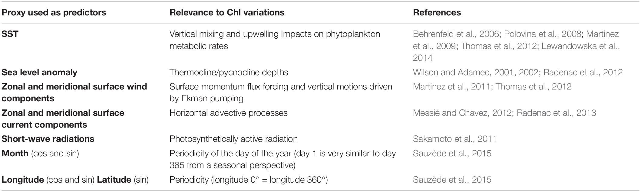
Table 1. Physical predictors, their relevance to Chl variations and associated references.
We purposely limited the predictors to surface variables because our objectives are (1) to reconstruct Chl from physical observations, which are mainly available through remotely sensed surface data (oceanic observations below the surface are indeed usually not accessible at large spatial-scales or interannual time-scales); (2) to build a statistical scheme that can complement more complex numerical models (here, NEMO-PISCES) which simulate complex three-dimensional processes and are costly to run.
A first SVR is trained on physical predictors from NEMO and DFS5.2 vs. ChlPISCES. The reconstructed Chl time-series is referred to as ChlSvr–PISCES. A second SVR is trained using the same physical predictors but vs. satellite Chl observations (ChlOC–CCI). The reconstructed Chl time-series is referred to as ChlSvr–CCI.
Climate Indices
Climate indices are provided by the National Oceanic and Atmospheric Administration (NOAA) website2 : the AMO, the Multivariate El Niño Southern Oscillation (ENSO) Index (MEI) and the Interdecadal Pacific Oscillation (IPO).
Support Vector Regression
The statistical reconstruction technique is based on a SVR. This method belongs to kernel methods in Statistical Learning Theory and relates to the Support Vector Machine (SVM, Vapnik, 1998). SVM is a kernel-based supervised learning method (Vapnik, 2000) developed for classification purpose in the early 1990s and then extended for regression by Vapnik (1995). The basic idea behind SVR is to map the variables into a new non-linear space using the kernel function, so that the regression task becomes linear in this space. The learning step estimates the parameters of the regression model according to a linear quadratic optimization problem, which can be solved efficiently. SVR also uses a robust error norm based on the principle of structural risk minimization, where both the error rates and the model complexity should be minimized simultaneously. Because SVR can efficiently capture complex non-linear relationships, it has been used in a variety of fields, and more specifically for oceanographic, meteorological and climate impact studies (Aguilar-Martinez and Hsieh, 2009; Descloux et al., 2012; Elbisy, 2015; Neetu et al., 2020), as well as in marine bio-optics (Kim et al., 2014; Hu et al., 2018; Tang et al., 2019).
Predictors and Chl are normalized by removing their respective average and dividing them by their standard deviations. Two SVR are trained over 1998-2010: one on ChlPISCES and one on ChlOC–CCI (Step A in Figure 1). This time period has been chosen as 1998 is the first complete year of the satellite ChlOC–CCI time-series, and 2010 is the last year available of the modeled ChlPISCES. The two resulting SVR schemes are applied on the NEMO-DFS5.2 physical predictors over 1979–2010. Finally, the annual means and standard deviations initially removed are applied to perform the back transformation and reconstruct either ChlSvr–PISCES or ChlSvr–CCI (Step B in Figure 1).
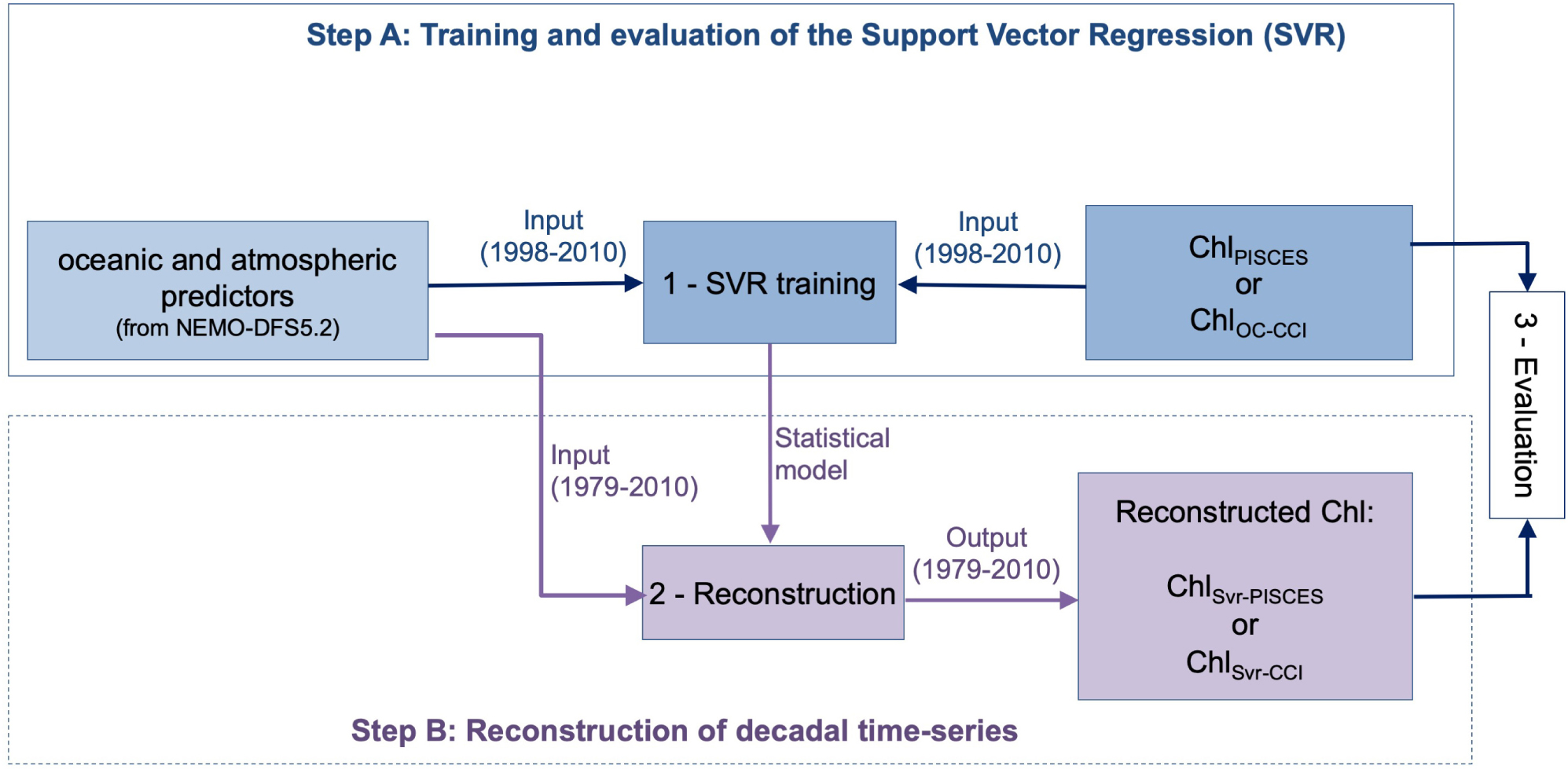
Figure 1. Steps performed to train the SVR and reconstruct Chl time-series.
Considering a Gaussian kernel, SVR only involves the selection of two hyperparameters: the penalty parameter C of the error term and the kernel coefficient gamma, driving the reduction of the cost function. C and gamma values are 1 and 0.1, respectively when the SVR is trained on ChlPISCES, and 2 and 0.3 when trained on ChlOC–CCI (see details in the Supplementary Material and Supplementary Figure 1A). Sensitivity tests to an increasing portion of the sample total number (from 0.2 to 9% of the full dataset) used in the training process are performed (see Supplementary Material and Supplementary Figure 1B). The mean absolute error stabilizes for a sample number higher than 6%, suggesting that the SVR skills don’t improve much afterward. This observation combined with computational limitations lead us to present the 9% experiment hereafter.
Empirical Orthogonal Function Analysis
The SVR skills to reconstruct Chl interannual to decadal variations are investigated performing Empirical Orthogonal Function analysis on ChlPISCES, ChlOC–CCI, ChlSvr–PISCES and ChlSvr–CCI. First, Chl data are centered and reduced (i.e., the monthly climatology is removed and the induced anomalies are divided by their standard deviations) to avoid an overly dominant contribution of high values on the analysis (Emery and Thomson, 1997) over the periods of interest (i.e., 1998–2010 or 1979–2010). A 5-month running mean is applied to focus on the interannual/decadal signal. The analysis is separately performed for the Atlantic, Pacific and Indian Oceans north of 40°S until 60°N, and for the 40°S–60°S region hereafter referred to as the Austral Ocean. Indeed, the large area covered by the Pacific Ocean and its dominant modes in climate variability (i.e., ENSO/IPO), could regionally dampen other modes of variability. Basin-scale spatial maps are then gathered to a global one, referred to as EOF. The associated time-series refer to as the Principal Components (PCs).
Synthetic Reconstruction From a Physical-Biogeochemical Ocean Model
This section assesses the reliability and robustness of the SVR approach using a complete and coherent dataset extracted from a global simulation performed with a coupled physical-biogeochemical ocean model. The SVR is first trained over 1998–2010 on ChlPISCES, and ChlSvr–PISCES is reconstructed over 1979–2010. ChlPISCES and ChlSvr–PISCES are then compared over 32 years to evaluate the consistency of the proposed data-driven reconstruction scheme.
Evaluation of ChlPISCES at Global Scale
The ability of the NEMO-PISCES model to reproduce the satellite Chl over 1998–2010 is briefly presented here. Boreal winter and summer climatology from ChlPISCES compare reasonably well with those of ChlOC–CCI (Figure 2A vs. 2B and 2C vs. 2D). The model correctly represents the main spatial patterns with, for instance, higher Chl and a stronger seasonal cycle at high latitudes, despite an overestimated biomass in the Southern Ocean (Launois et al., 2015). The model also captures low Chl in the subtropical gyres, with some underestimation. This discrepancy may be explained by the lack of acclimation dynamics to oligotrophic conditions or by the assumption of constant stoichiometry either in phytoplankton or in organic matter in the model (Ayata et al., 2013; Aumont et al., 2015). The model underestimates Chl values in the equatorial Atlantic and Arabian Sea. In this latter region, mesoscale and submesoscale processes unresolved by the model have been shown to be of critical importance (Hood et al., 2003; Resplandy et al., 2011). Finally, the parameterization of nitrogen-fixing organisms not explicitly modeled in that PISCES version could explain the ChlPISCES underestimation in the western Pacific in austral summer (Dutheil et al., 2018).
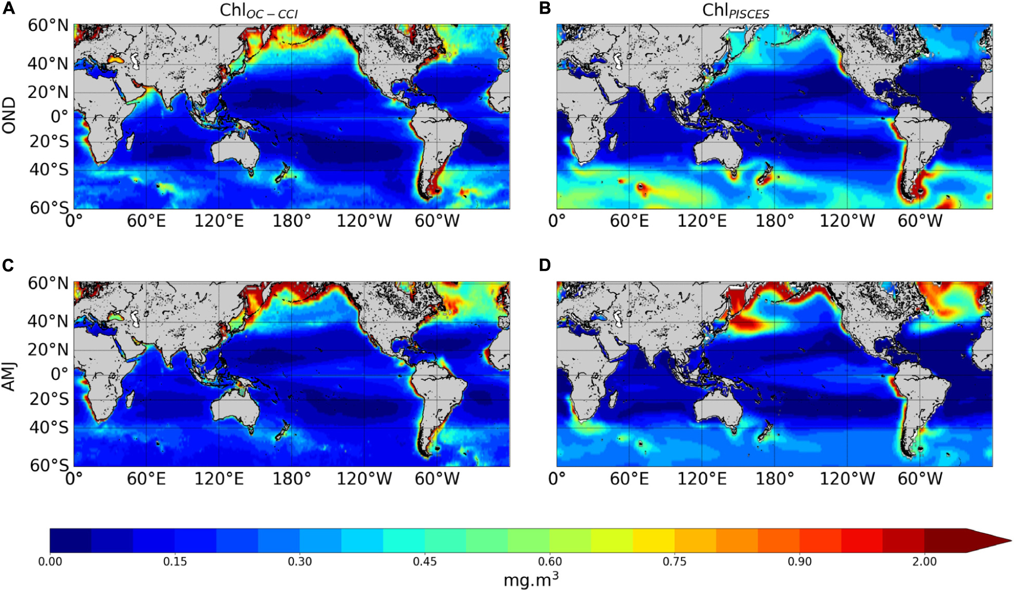
Figure 2. Surface seasonal mean of Chl (mg.m–3) over 1998–2010 derived from satellite (left panels) and the PISCES model (right panels), in October–November–December (A,B) and April–May–June (C,D).
High Chl are accurately simulated in the eastern boundary upwelling systems. In two of the three main High Nutrient Low Chlorophyll (HNLC) regions, i.e. the equatorial Pacific and the eastern subarctic Pacific, the model successfully reproduces the moderate ChlOC–CCI. However, the model overestimates ChlOC–CCI east of Japan because of an incorrect representation of the Kuroshio current trajectory. This common bias in coarse resolution models (i.e., Gnanadesikan et al., 2002; Dutkiewicz et al., 2005; Aumont and Bopp, 2006) is potentially related to too deep mixed layer simulated in winter inducing very strong spring blooms (Aumont et al., 2015). In the Southern Ocean, the third and largest main HNLC region, the model overestimates ChlOC–CCI values, especially during summer. However, the standard satellite algorithms that deduce Chl from reflectance tend to underestimate in situ observations by a factor of about 2–2.5, especially for intermediate concentrations (e.g., Dierssen and Smith, 2000; Kahru and Mitchell, 2010). It is to note that Chl in physical-biogeochemical coupled models is commonly overestimated in the Southern Ocean, and systematically underestimated in the oligotrophic gyres (Séférian et al., 2013).
The 1st mode of the EOF analysis performed on interannual Chl displays close percent of total variance for ChlOC–CCI and ChlPISCES (16.6% vs. 21.1%, respectively). Their PCs in the Pacific Ocean are well correlated with the MEI (r = 0.71 and 0.89 with p = 0.0015 and p < 0.001, respectively; Figure 3C). PCs show the greatest positive values in January 1998 during the peak of the strong 1997/1998 El Niño event and the greatest negative values during the following La Niña beginning of 1999. The associated EOFs display a Chl horseshoe pattern (Figures 3A,B), reminiscent of the ENSO pattern on SST (Supplementary Figure 2; Messié and Chavez, 2012). While the tropical Pacific experiences a Chl decrease during El Niño events, the North and South Pacific display a Chl increase, and inversely during La Niña. This typical ENSO pattern is also related to remote Chl anomalies outside the Pacific induced by atmospheric teleconnections, such as a Chl decrease in the tropical North Atlantic and in the South Indian Ocean during El Niño. Although the Atlantic and Indian Ocean’s PCs are not correlated with the MEI (0.14 and 0.05, respectively), their EOFs are similar to those obtained from analysis performed at global scale (vs. basin scale here) and which have been largely discussed in the past (e.g., Behrenfeld et al., 2001, 2006; Yoder and Kennelly, 2003; Chavez et al., 2011). ChlPISCES reasonably well captures the first mode of ChlOC–CCI interannual variability over 1998–2010 in the Pacific and Atlantic Oceans, with 0.89 and 0.77 (p < 0.001) correlations between their PCs, respectively, but not in the Indian Ocean, where the PCs correlation is far weaker (0.13) and insignificant (Figures 3C–E).
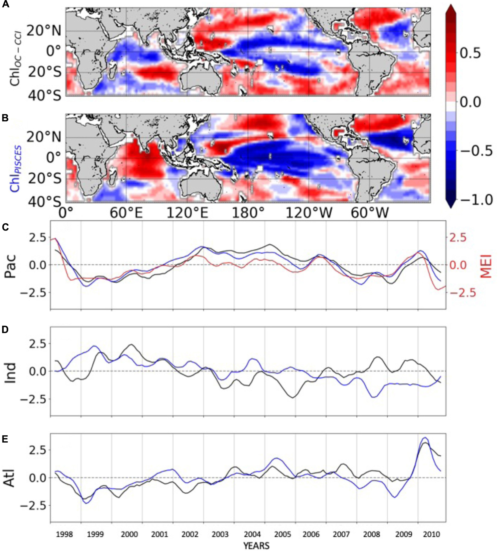
Figure 3. First mode of basin-scale EOFs of interannual (A) ChlOC–CCI and (B) ChlPISCES, and their corresponding PCs over 1998–2010 in the (C) Pacific, (D) Indian and (E) Atlantic Oceans. ChlOC–CCI and ChlPISCES PCs are represented by the black and blue lines, respectively. The MEI index is reported in red (right y-axis) on (C).
Evaluation of the SVR Method Trained on Synthetic Data Only
Statistical Performances
A first evaluation of the SVR applied on the synthetic dataset (i.e., both physical and biogeochemical model outputs) is provided for the dedicated subset (i.e., 20% of 9% of the total data set) over the 1998–2010 training time period. ChlPISCES and ChlSvr–PISCES datasets display a determination coefficient of 0.95 and a root mean square error (RMSE) of 0.22 (see Supplementary Figure 1C), indicating at first glance a very good ability of the SVR to reconstruct ChlPISCES. The SVR reconstruction is very accurate when comparing the full modeled and reconstructed Chl for (i) the 1998–2010 training time period, (ii) the 1979–1997 fully independent dataset, and (iii) the 1979–2010 whole dataset, both at global and basin scales (Table 2 and Figure 4). For each oceanic basin, determination coefficients between both datasets over 1979–1997 exceed 0.84, except in the Austral Ocean where they get down to 0.71. RMSE are lower than 0.14 and associated with a slope ranging from 0.84 in the Austral to 0.97 in the Atlantic (Figure 4). In addition, the quality of the reconstructed ChlSvr–PISCES over the 1979–1997 independent time period is only marginally degraded compared to the 1998–2010 training period or the 1979–2010 full period.
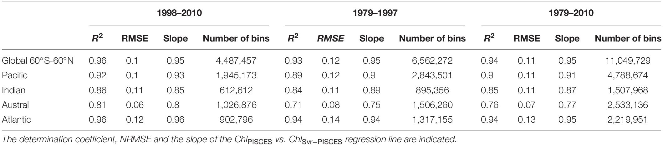
Table 2. Statistical performances between ChlPISCES vs. ChlSvr–PISCES normalized monthly anomalies for the global ocean and the 4 oceanic basins over the 1998–2010, 1979–1997, and the whole 1979–2010 time period.
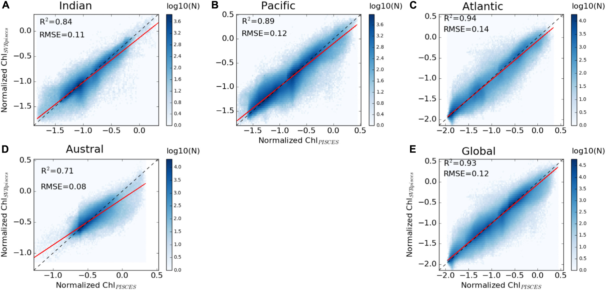
Figure 4. Scatter plots of ChlPISCES vs. ChlSvr–PISCES normalized monthly anomalies over 1979–1997, (A–D) for each basin and (E) at global scale between 60°S and 60°N. The ChlPISCES vs. ChlSvr–PISCES and the 1:1 regression lines are plotted as the continuous red and dash black lines, respectively. The figure is color-coded according to the density of observations.
Evaluation of the Reconstructed Chl Spatio-Temporal Variability
The Normalized Root-Mean-Square-Error (NRMSE, i.e., RMSE normalized by the average Chl used to train the SVR) between ChlPISCES and ChlSvr–PISCES filtered with a 5-month running mean (to discard the high frequency signal) shows an error ranging between 10 and 20% over 1998–2010 (Figure 5A). Their correlation exceeds 0.7 (p < 0.001) over most of the global ocean (Figure 5B). At mid-latitudes they are generally larger than 0.8, and they range between 0.6 and 0.9 in the equatorial Pacific. This accurate reconstruction demonstrates that a strong relationship exists between physical processes and Chl at global scale. However, the reconstructed Chl field can be regionally less accurate. For instance, the edges of the oligotrophic gyres (delimited by the 0.1 mg.m–3 contour in Figure 5A) exhibit the highest NRMSE and lowest correlations. Large NRMSE are also evident in the Gulf Stream region while the western tropical Atlantic exhibits lower correlations than 0.5.
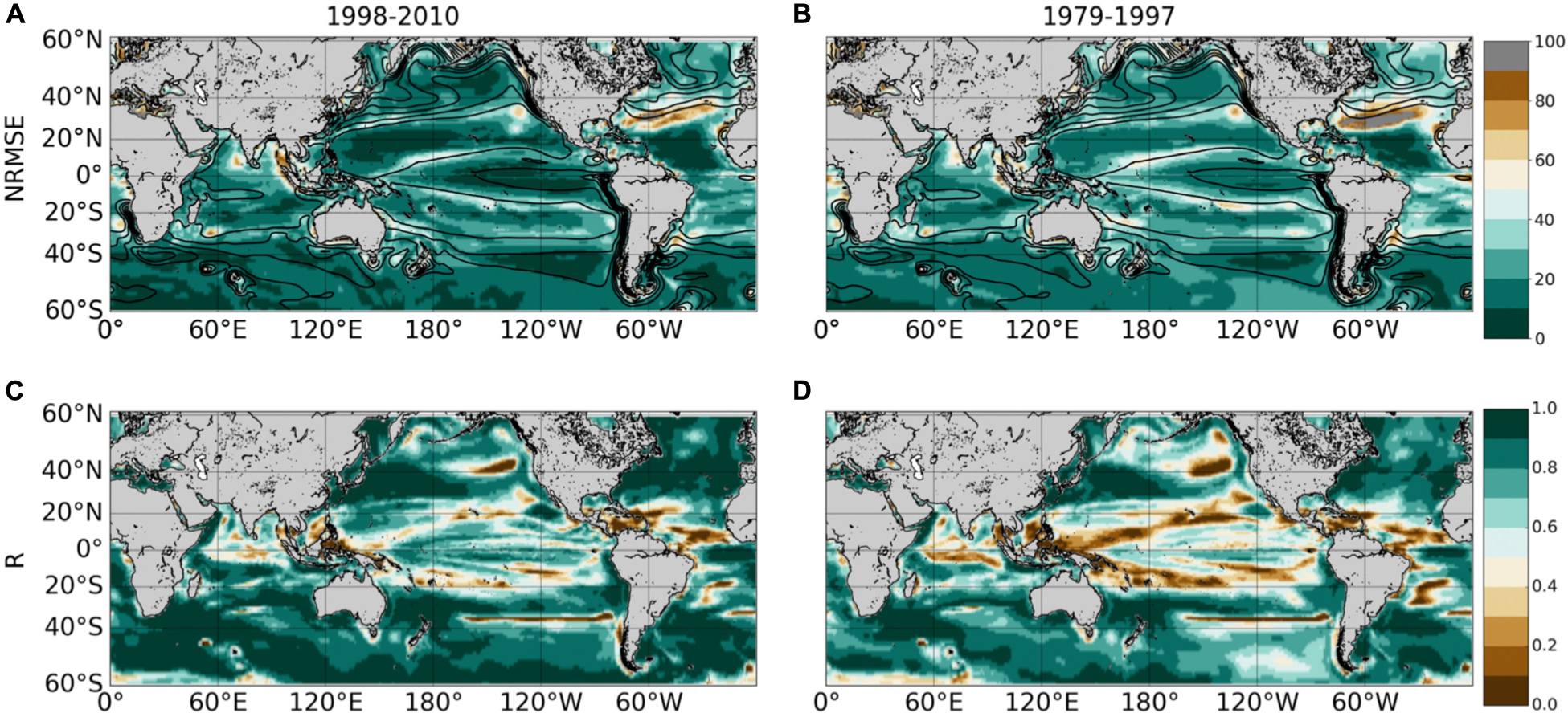
Figure 5. (A,B) NRMSE (in%) and (C,D) correlation between ChlPISCES vs. ChlSvr–PISCES after applying a 5 month-running mean on both time-series. These 2 diagnostics are calculated over 1998–2010 (left column) and 1979–1997 (right column). Contours on the upper panels show their respective 1998–2010 Chl time average (every 0.1 mg.m–3).
Those discrepancies could be due first to the zooplankton grazing pressure (top–down control) which is often overestimated in PISCES simulations. It results in an underestimated nanophytoplankton biomass in the oligotrophic gyres, emphasized along their edges (Laufkötter et al., 2015). Because the top–down control is not accounted for by the SVR, Chl variability induced by the overgrazing in these areas might not be captured. Second, in the equatorial Pacific Ocean, a minimum iron threshold value has been imposed (0.01 nmol.L–1) in the biogeochemical model. Without that threshold Chl is too low on both sides of the equator, resulting in a strong accumulation of macronutrients and a spurious poleward migration of the subtropical gyre boundaries (Aumont et al., 2015). While the existence of such a threshold suggests that a minor but regionally important source of iron is missing in PISCES, it also suggests the inability of the SVR in reproducing ecosystem dynamics related to such artificial input of micro-nutrient. Finally, atmospheric input of iron through desert dust deposition is known to be stronger in the Atlantic than in the Pacific Ocean (Jickells et al., 2005). Such signal cannot be accounted for by the SVR with the given predictors, which might (with meso – and sub-mesoscale activities) explain the higher NRMSE in the north western Atlantic than in the north-western Pacific.
As expected, areas of high NRMSE and low correlations between ChlPISCES and ChlSvr–PISCES identified over 1998–2010 (Figure 5, left column) extend and strengthen over 1979–1997 (Figure 5, right column). Indeed, the correlations significantly decrease in the tropical Pacific while they slightly decrease in mid-latitudes between the two periods. Correlations remain high and NRMSE low in the North-West Pacific, North and South-West Atlantic, and South Indian Oceans as well as over a large part of the Southern Ocean providing confidence for analyses extended beyond the training period of the SVR.
The analysis is now extended to the 1979–2010 time-period to investigate the skills of the SVR in reproducing phytoplankton interannual/decadal cycles. The 1st EOFs of ChlPISCES vs. ChlSvr–PISCES have the same sign of variability over 72% of the global ocean (Figures 6A,B). Both EOFs are similar in the Pacific and Atlantic Oceans and their PCs are highly correlated over 1979-2010 (Table 3 and Figures 6C,E). In the Pacific, these EOFs strongly resemble the typical horseshoe pattern of IPO with SST anomalies of opposite polarities in the tropical and extra-tropical Pacific regions (Supplementary Figure 3). Correlations between ChlPISCES and ChlSvr–PISCES 1st PCs and the IPO index are high (0.94 and 0.95 with p < 0.001, respectively; blue and black vs. red lines in Figure 6C). It highlights that the 1st mode of Chl variability in the Pacific is strongly driven by the IPO. In the Atlantic, both PCs are strongly correlated with the AMO (−0.8 for ChlSvr–PISCES and −0.85 for ChlPISCES with p < 0.001; Figure 6E). The AMO shifts from a cold to a warm phase in the mid-1990’s (Supplementary Figure 3), and is associated with a decrease in Chl (Figures 6A,B).
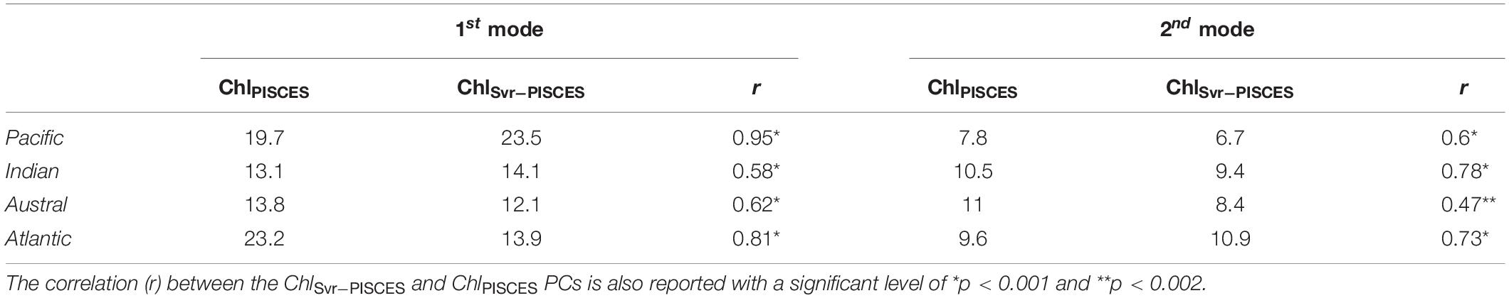
Table 3. Percent variance explained by the first two modes of the Empirical Orthogonal Function analysis performed on ChlPISCES and ChlSvr–PISCES for each oceanic basin over 1979–2010.
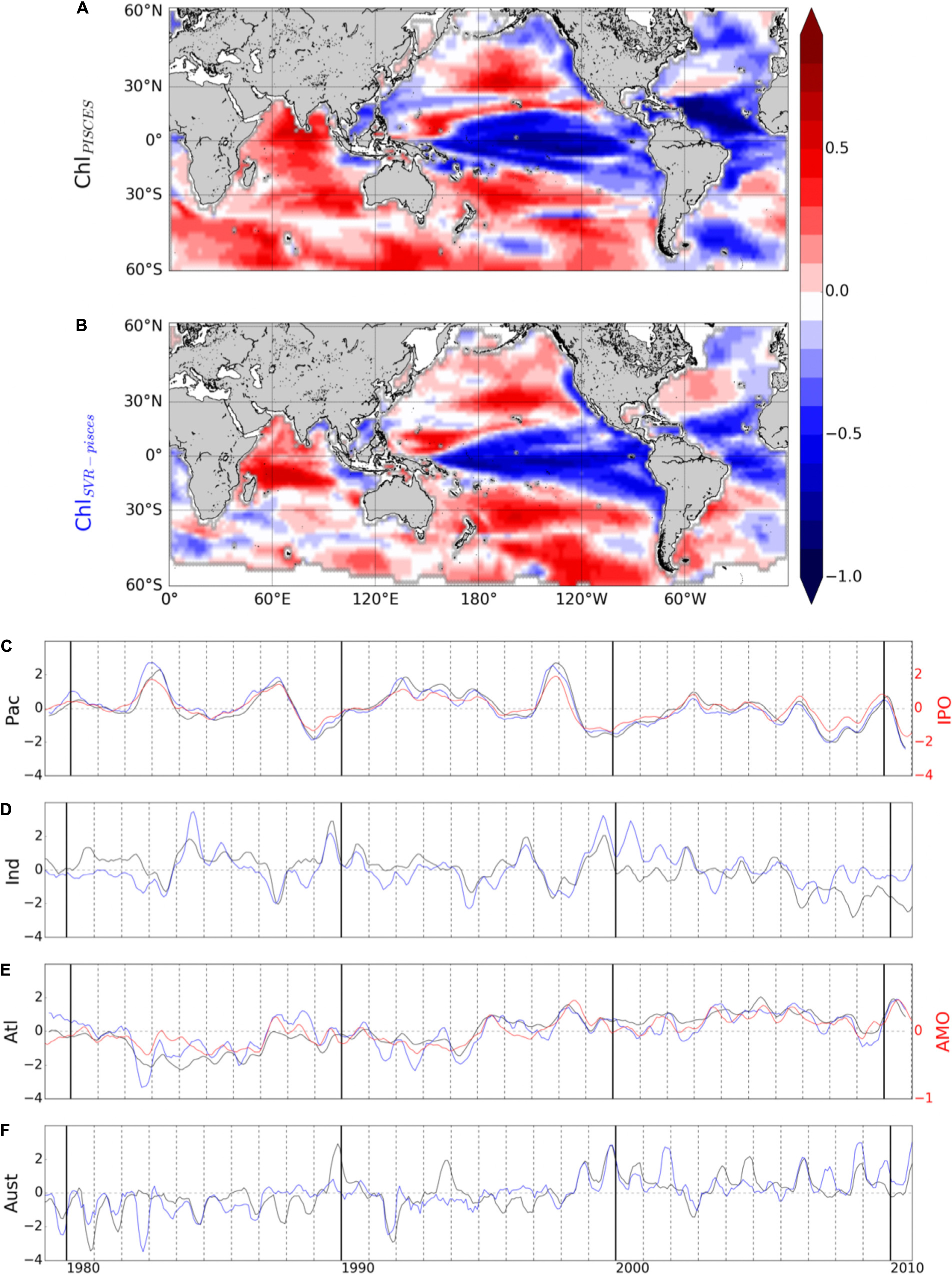
Figure 6. First mode of basin-scale EOFs of interannual (A) ChlPISCES and (B) ChlSvr–PISCES, and their corresponding PCs over 1979–2010 in the (C) Pacific, (D) Indian, (E) Atlantic, and (F) Austral Oceans (black and blue lines, respectively). Climate indices are reported in red (right y-axis).
The 1st two modes explain a similar percent variance for ChlPISCES and ChlSvr–PISCES in the four oceanic basins, with the exception of the 1st mode in the Atlantic Ocean (see Table 3). In this basin ChlSvr–PISCES percent variance is underestimated by a factor 2 compared to ChlPISCES, while their 1st EOFs and PCs are well correlated. One explanation might be that the AMO is the climate cycle with the longest period (80 years) when compared to the IPO. Thus, it might be the most difficult signal to reproduce as the SVR is trained over a relatively “short” 12 years’ time-period.
The agreement between ChlPISCES and ChlSvr–PISCES 1st mode is not as good in the Austral and Indian Oceans when compared to the Atlantic and Pacific Oceans (Table 3 and Figures 6A,B,D,F). In the Indian Ocean, the ChlPISCES EOF exhibits a maximum positive variability along the western Arabian Sea, while it is located north-east of Madagascar for ChlSvr–PISCES. In the Austral Ocean, ChlPISCES and ChlSvr–PISCES EOFs roughly follow a zonal distribution.
A strong correspondence between SST and Chl has been previously reported over a large part of the global ocean (Behrenfeld et al., 2006; Martinez et al., 2009; Siegel et al., 2013), demonstrating the close interrelationship between ocean biology and climate variations. Consequently, it is not surprising to observe strong correlations between ChlPISCES or ChlSvr–PISCES and climatic indexes mostly built on SST anomalies (Supplementary Figure 3).
The 2nd mode of variability of ChlPISCES is also well reproduced by the SVR. The percent variances are close (Table 3) as well as their spatio-temporal variability in the four oceanic basins (Supplementary Figure 4). The high correlations between the first two modes of ChlPISCES vs. ChlSvr–PISCES highlight the SVR ability to relatively well reproduce the ChlPISCES low-frequency variability.
Application to Satellite Radiometric Observations
SVR Statistical Performances and Sensitivity Tests
In this section, the SVR uses the same physical predictors from NEMO-DFS5.2 as in Section “Synthetic reconstruction from a physical-biogeochemical ocean model,” but it is trained on satellite radiometric observations (e.g., ChlOC–CCI). The same procedure is followed (see Supplementary Figures 5A,B). A first validation is performed for 20% of 9% of the full data set and over the 1998–2010 training period showing a high determination coefficient of 0.87 and RMSE of 0.37 between ChlOC–CCI and ChlSvr–CCI (Supplementary Figure 5C).
As expected, the regression lines between the whole dataset of ChlOC–CCI vs. ChlSvr–CCI for each oceanic basin and at global scale are farther away from the 1:1 line than for the synthetic study over the training period, but still remain close (higher slope than 0.8, except in the Austral Ocean; Figure 7). The SVR trained on NEMO-DFS5.2 predictors vs. satellite Chl is expected to be less efficient than the SVR trained on the coherent NEMO-DFS5.2-PISCES physical-biogeochemical dataset. Some of the biological interactions/processes (such as the diversity of the prey-predator relationships, the complexity of photoacclimation phenomena) are not yet optimally formulated by model equations inducing that Chl derived from numerical modeling is oversimplified compared to the complexity of the real ocean. Not to mention that satellite Chl may itself be partially affected by other components that are not Chl, such as colored dissolved organic matter (CDOM; Morel and Gentili, 2009) and suspended particulate matter (SPM). Phytoplankton can also adjust their intracellular Chl according to light and nutrient availability (e.g., Laws and Bannister, 1980; Behrenfeld et al., 2015). The induced Chl changes are no longer ascribed to changes in biomass. All these signatures on satellite Chl could explain ChlSvr–CCI underestimation. Nevertheless, determination coefficients between ChlSvr–CCI and ChlOC–CCI remain high over the training time period (0.85, 0.89, and 0.86 for the Indian, Pacific and Atlantic Oceans, respectively, Figure 7).
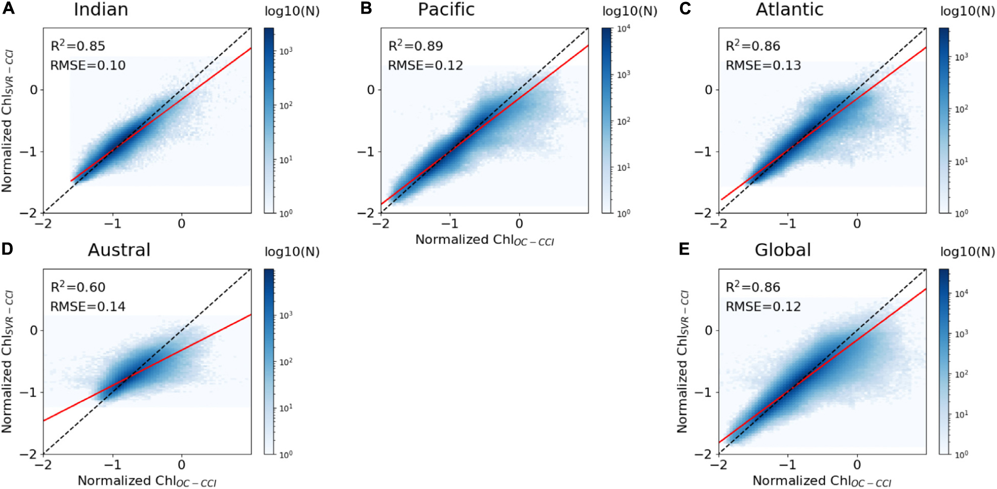
Figure 7. Scatter plots of ChlOC–CCI vs. ChlSvr–CCI normalized monthly anomalies over 1998–2010, (A–D) for each basin and (E) at global scale between 60°S and 60°N. The ChlOC–CCI vs. ChlSvr–CCI and the 1:1 regression lines are plotted as the continuous red and dash black lines, respectively. The figure is color-coded according to the density of observations.
The NRMSE between ChlOC–CCI vs. ChlSvr–CCI is lower than 20% over most of the global ocean (Figure 8A). Correlations higher than 0.9 (p < 0.001) are evident over large subtropical areas in the Atlantic, Indian and Pacific Oceans as well as in the Equatorial Pacific (Figure 8B). Interestingly, the SVR generally does a better job at reconstructing the satellite Chl than the modeled one (Figures 5A,C vs. Figure 8). NRMSE are higher at high latitudes and along the oligotrophic area boundaries, although to a less extent than for ChlPISCES. Because ChlOC–CCI can only be retrieved under clear sky conditions, gaps in satellite observations (especially during wintertime) likely alters the SVR learning and could explain such a degradation of ChlSvr–CCI as moving toward high latitudes.
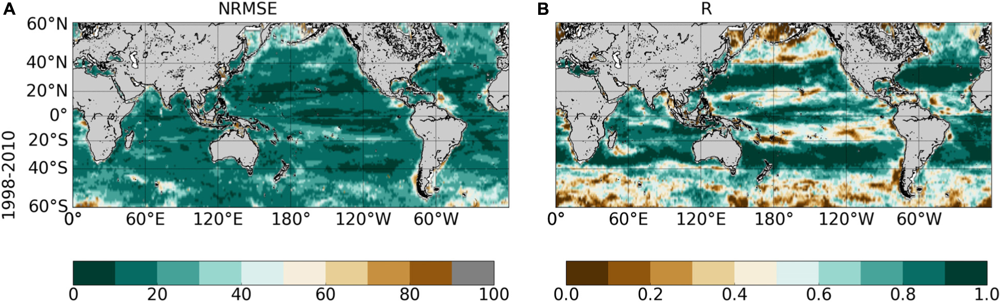
Figure 8. (A) NRMSE (in%) and (B) correlation between ChlOC–CCI vs. ChlSvr–CCI over 1998–2010 after applying a 5 month-running mean on both time-series. Contours on the NRMSE show the 1998–2010 ChlOC–CCI time average (every 0.1 mg.m–3). Correlations < 0.73 and 0.6 are significant with a p-value < 0.001 and 0.01, respectively.
Reconstruction of Satellite Chl Interannual to Decadal Variability and Trends
The SVR ability to replicate ChlOC–CCI interannual variability is now investigated over 1998–2010 (Figure 9). In the Pacific Ocean, ChlOC–CCI and ChlSvr–CCI 1st EOFs are close (Figure 9A vs. 9B), their PCs are highly correlated (r = 0.89, p < 0.001; Figure 9C), and their percent variance are similar (Table 4). As presented in Section “Evaluation of ChlPISCES at global scale,” this mode of Chl variability can be attributed to ENSO, given their EOFs pattern as well as their PCs highly correlated with the MEI (rOC–CCI/MEI = 0.71 and rSvr–CCI/MEI = 0.91, with p = 0.0015 and p < 0.001, respectively). Interestingly, ChlSvr–CCI EOFs are closer to ChlOC–CCI than ChlPISCES in several areas such as in the north-western Pacific, the south-western Atlantic and the Indian Ocean from Madagascar to the western coast of Australia (Figures 9A,B vs. Figure 3B). Consistently, correlations between ChlOC–CCI and ChlSvr–CCI PCs in the three basins and for the 1st two modes are higher than between ChlOC–CCI and ChlPISCES (Table 4).
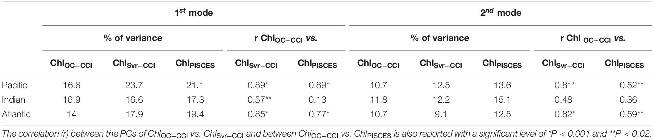
Table 4. Percent variance explained by the first two modes of the Empirical Orthogonal Function analysis performed on ChlOC–CCI, ChlSvr–CCI, and ChlPISCES for each oceanic basin over 1998–2010.
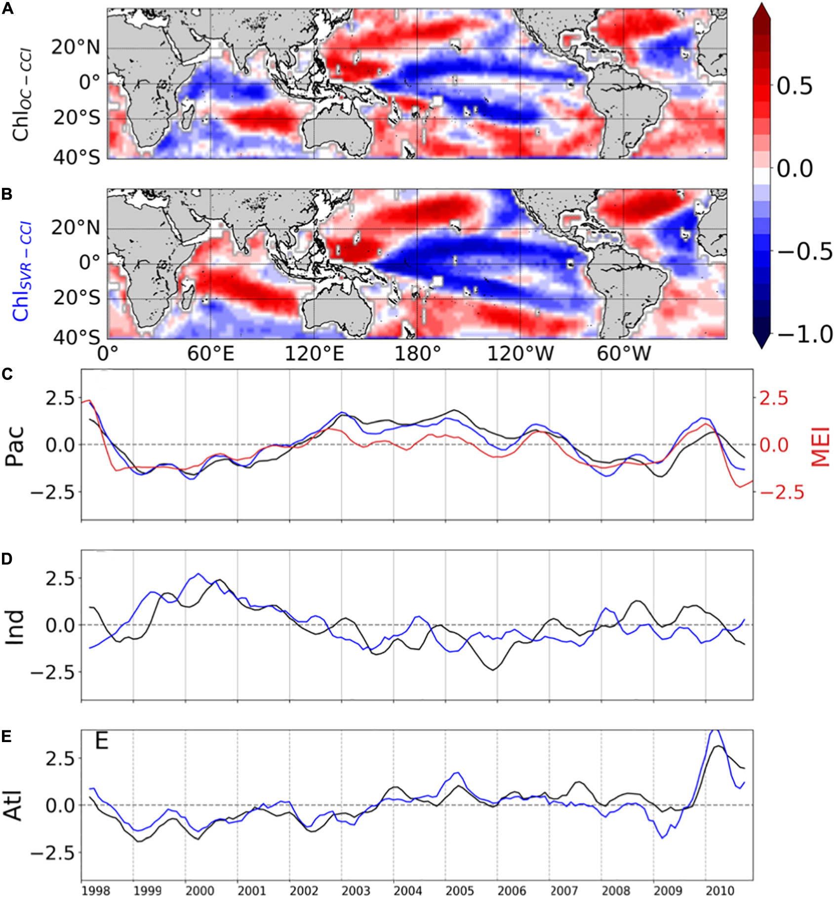
Figure 9. First mode of basin-scale EOFs of interannual (A) ChlOC–CCI and (B) ChlSvr–CCI and their associated PCs over 1998–2010 in the (C) Pacific, (D) Indian, and (E) Atlantic Oceans as the black and blue lines, respectively (left y-axis). The climate indices are reported in red on the right y-axis.
ChlOC–CCI linear trends over 1998–2010 exhibit large areas of increase or decrease (red and blue areas in Figure 10A, respectively). Productive regions at high latitudes and along the equatorial and upwelling areas generally exhibit positive ChlOC–CCI trends, albeit many underlying regional nuances. Contrastingly, trends are generally negative in the center of the gyres. These regional trends are consistent with those extracted from the first 13 years of the SeaWiFS record and discussed by Siegel et al. (2013) (see their Figures 5B, 8B). The negative trends in the oligotrophic gyres were also reported by Signorini et al. (2015) who attributed this behavior to MLD shallowing trends. Surface water density variability induced by changes in temperature and salinity, combined with wind stirring, are effective drivers of vertical mixing, which in turn control the renewal of nutrients from the rich-deep layers toward the euphotic zone. Thus, shallower MLD would decrease nutrient uplift and phytoplankton growth in the oligotrophic areas.
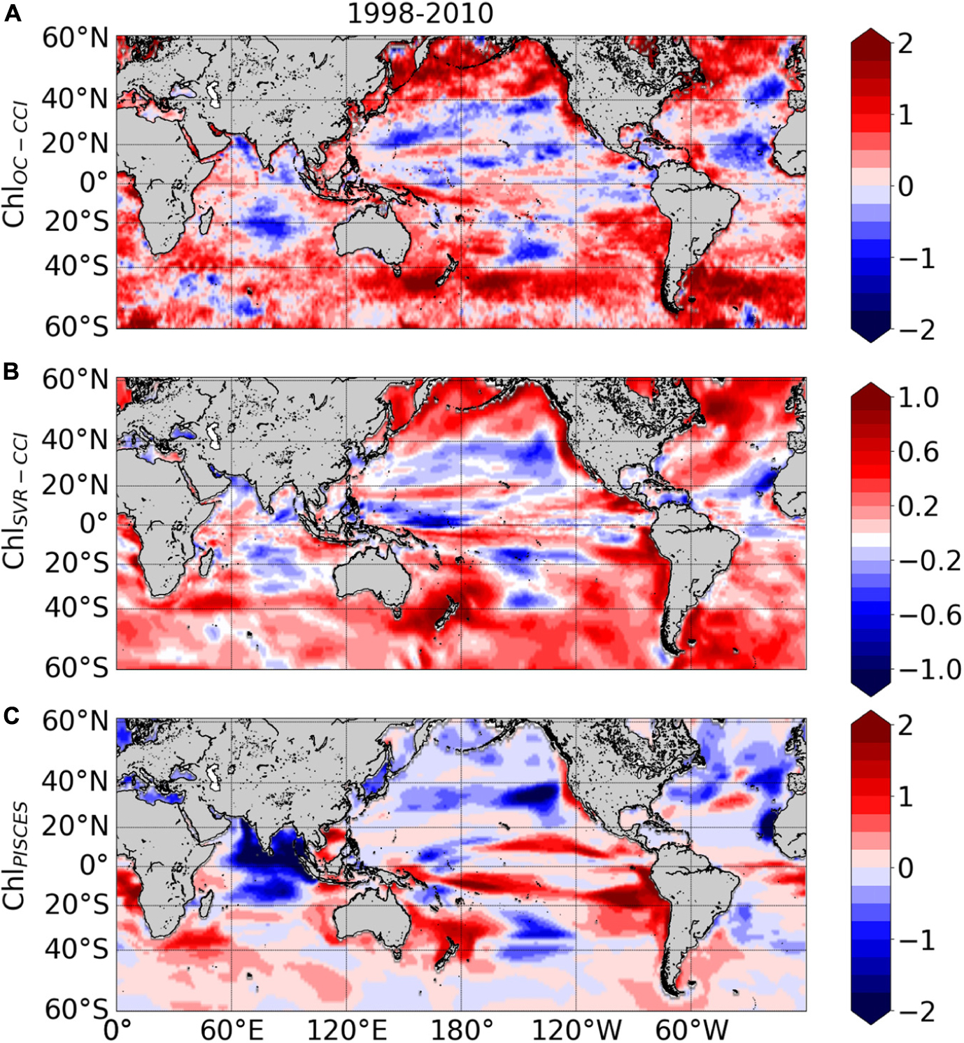
Figure 10. Linear trends (in% year –1) calculated over 1998–2010 from the monthly (A) ln(ChlOC–CCI), (B) ln(ChlSvr–CCI), (C) ln(ChlPISCES). Note that the scale is divided by 2 for ln(ChlSvr–CCI).
ChlSvr–CCI trends agree qualitatively well with those of ChlOC–CCI at global scale (Figure 10B vs. 10A, respectively). Indeed, decline of ChlSvr–CCI can be observed in the center of the gyres, while outside ChlSvr–CCI generally increases in a similar way to ChlOC–CCI. ChlSvr–CCI accurately captures the largest ChlOC–CCI increase observed in the Southern Ocean along the Antarctic Circumpolar Current. While Gregg and Casey (2004) reported a substantial negative bias in the SeaWiFS data for this region when compared to in situ observations, which could hamper the reliability of satellite trends discussed in this area (e.g., Siegel et al., 2013), the SVR remains able to reproduce the positive observed trend. Despite qualitative spatial agreements, it is noteworthy that the SVR underestimates by half the magnitude of the satellite trend (see scales in Figure 10A vs. 10B).
Interestingly, trends in ChlPISCES generally differ from ChlOC–CCI (Figure 10C). This is striking for the North Pacific and Atlantic high latitudes, but also in the equatorial Atlantic and Arabian Sea with opposite trends when compared with ChlOC–CCI and ChlSvr–CCI, and in a more mitigated manner in the Austral Ocean.
ChlSvr–CCI is also compared with the only historical consistent dataset built by Antoine et al. (2005) who reanalyzed ocean color time series from CZCS (1979–1983) and SeaWiFS (1998–2002). A 22% global mean increase of Chl between the two era was reported. It was mainly due to large increases in the intertropical areas and to a lesser extent in higher latitudes, while oligotrophic gyres displayed declining concentrations (Figure 11A). SST from the SODA reanalysis was used as a proxy of ocean stratification and opposite Chl and SST changes over 60% of the ocean between 50°S and 50°N was reported (light blue and yellow in Figure 11B, adapted from Martinez et al., 2009). This inverse relationship was used to hypothesized that multidecadal changes in global phytoplankton abundances were related to basin-scale oscillations of the ocean dynamics. Briefly, SST changes were related to a regime shift of the PDO (although the use of the basin-scale IPO would have been more appropriate) from a warm to a cold phase in the Pacific and Indian Oceans leading to an increase of Chl, and inversely in the Atlantic Ocean with a regime shift from a cold to a warm phase of the AMO leading to a Chl decrease.
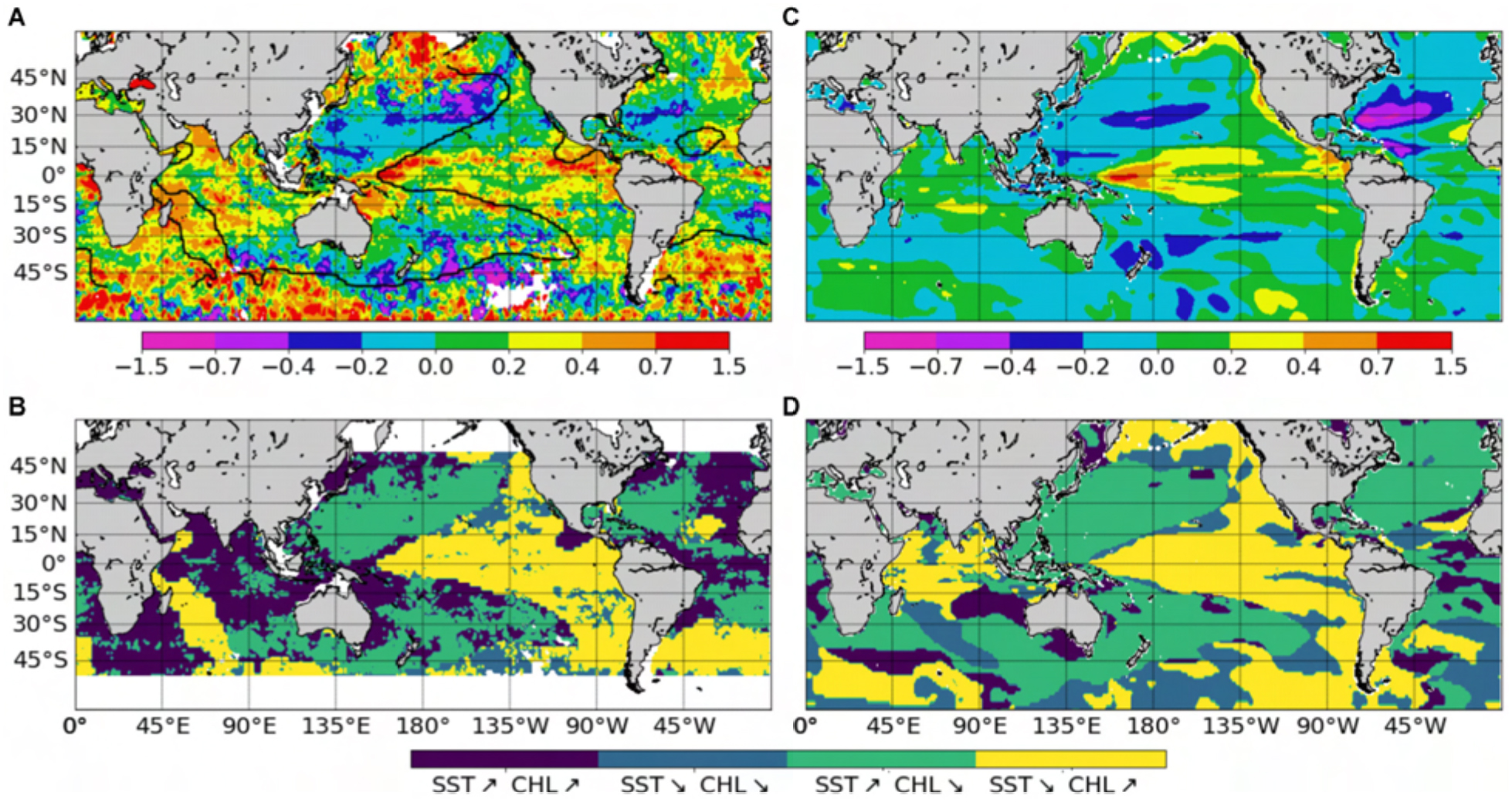
Figure 11. Chl change from the CZCS (1979–1983) to the SeaWiFS (1998–2002) era, expressed as the logarithm of the ratio of the average values over the two time periods (A) from satellite Chl adapted from Antoine et al. (2005), (C) from ChlSvr–CCI. Note that this ratio is multiplied by 2 to fit the same color bar as in (A). Maps of areas with concomitant parallel or opposite changes of Chl and SST (B) from Chl satellite and SST from the SODA reanalysis adapted from Martinez et al. (2009) and (D) from ChlSvr–CCI and SSTNEMO. The respective SST zero differences are shown on the maps as a thick black curve.
Observed Chl changes over the last decades are accurately reproduced by ChlSvr–CCI, including a Chl increase in the equatorial Pacific and the southern tropical Indian Oceans, as well as a Chl decline in both the Atlantic and Pacific oligotrophic gyres (Figure 11C). However, the magnitude of the SVR reconstructed Chl is underestimated (note that the Chl ratio is multiplied by 2 in Figure 11C to allow the comparison with Figure 11A). On average, the inverse relationship between ChlSvr–CCI and SSTNEMO (Figure 11D) occurs over 69.4% of the global ocean between 50°S and 50°N in a similar way to that reported by Martinez et al. (2009), especially in the Pacific Ocean (see Figure 11D vs. 11B). In the Indian Ocean, although Chl mainly increases in both studies, it is here associated with a SST decrease. Interestingly, this inverse Chl-SST relationship in the Indian Ocean (yellow area in Figure 11D) was reported in Behrenfeld et al. (2006) over the SeaWiFS era, suggesting that the SST dataset used in Martinez et al. (2009) may have decadal discrepancies for this region.
In their study, Martinez et al. (2009) analyzed two 5-year time periods apart from each other by 15 years. They suggested that averaging observations separately over the two time-periods may have dampen the effect of interannual variability and reveal the decadal one. Most of the changes observed between the time periods covered by the two satellites are here confirmed based on the reconstructed ChlSvr–CCI. However, the continuous 30-year time series of ChlSvr–CCI provides new insights on the observed regime shifts (Figure 12). In the Pacific Ocean, the 1st EOF of ChlSvr–CCI (Figure 12A) is close to the Chl spatial patterns obtained from the CZCS to SeaWiFS era (Figure 11C) and the PC remains highly correlated with the IPO over 1979-2010 (r = 0.94 with p < 0.001, Figure 12B). The Chl increase in the Indian Ocean, north-east of Madagascar toward the west coast of Australia, between the 1980’s and the 2000’s also appears on the ChlSvr–CCI EOF. These temporal changes might also be related to the IPO variability (correlation between the IPO index and ChlSvr–CCI PC = 0.6, p < 0.001; Figure 12C).
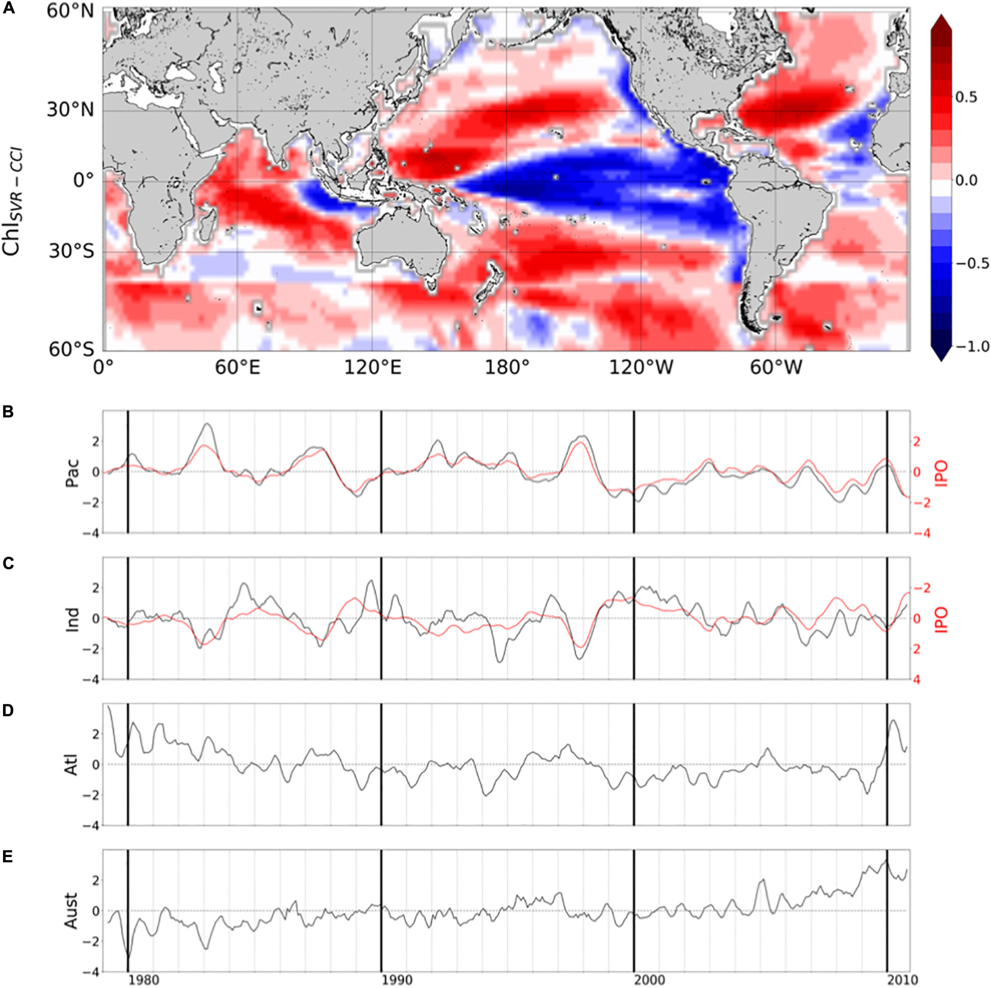
Figure 12. (A) 1st mode of basin-scale EOFs of interannual ChlSvr–CCI over 1979–2010 and their corresponding PCs in the (B) Pacific (23.2% of the total variance), (C) Indian (15.2% of the total variance), (D) Atlantic (13.5% of the total variance) and (E) Austral Oceans (11.4% of the total variance). IPO is reported in red (right y-axis).
In the Atlantic Ocean, CZCS-SeaWiFS Chl and ChlSvr–CCI 1st EOF also share some similarities, including a decrease of Chl in the subtropical gyres and an increase in the equatorial/tropical regions. The associated PC (Figure 12D), exhibits a shift between 1979–1983 and 1998–2002 consistently with Figure 2C of Martinez et al. (2009). In this latter study, this change was attributed to a regime shift of the AMO. However, the AMO index is not correlated with the 1st ChlSvr–CCI PC (r = 0.03, p = 0.43) but rather with the 2nd mode (r = 0.43 with p = 0.003, Supplementary Figure 6), likely explaining the spatial discrepancies in Figure 11A vs. 11C. Although the detailed analysis of Chl decadal variability is beyond the scope of the present study, these initial findings underscore the importance of continuous time series at regional/global scales to combine spatial and temporal information’s and properly investigate Chl long-term variability.
Summary and Conclusion
In this paper, we assess the efficiency of a machine learning statistical approach based on support vector regression to reconstruct surface Chl from oceanic and atmospheric variables. We first apply this strategy on a self-consistent global dataset gathering physical predictors and Chl data simulated by a coupled physical-biogeochemical model simulation. Our results indicate that this non-linear method accurately hindcasts interannual-to-decadal variations of the phytoplankton biomass simulated at global scale by the model, except at the boundaries of the subtropical gyres where the strong top-down control of zooplankton grazing in the numerical model is not accounted for by the SVR. Likewise, this statistical approach cannot yet reproduce Chl variability induced by nutrient inputs that are not directly related to our selected physical predictors, such as atmospheric iron deposit.
The SVR was then trained on satellite Chl observations. It accurately reproduces observed interannual Chl variations in most regions, including El Niño signature in the tropical Pacific and Indian Oceans as well as the main modes of Atlantic Chl variability. Despite an amplitude underestimation by half, it also accurately captures spatial patterns of Chl trends over the satellite period, with a Chl increase in most extratropical regions and a Chl decrease in the center of the subtropical gyres, as well as their changes between the CZCS and SeaWiFS era. Interestingly, while ChlPISCES magnitude is closer to ChlOC–CCI than ChlSvr–CCI, interannual variability and spatial trends of ChlPISCES are farther than ChlSvr–CCI to ChlOC–CCI. Equations representing the processes that govern the evolution of biogeochemical variables in a biogeochemical model are obviously less complex than the ones at play in the real ocean. We thus anticipated the modeled Chl to be easier to reconstruct than the satellite one. Additional complications were also expected through the reconstruction of satellite Chl from the model oceanic and atmospheric predictors, which may be less realistic than physical parameters derived from satellite measurements. As a consequence, the SVR is indeed slightly less efficient at reproducing the major satellite Chl patterns compared to the model ones but is surprisingly more efficient at capturing observed Chl temporal variations. This results in a NRMSE generally weaker when reconstructing satellite data compared to the model one, although the predictors used are identical.
Machine learning techniques are powerful tools to statistically model non-linear processes. They require a significant amount of data to be trained and are well-suited to analyze remote sensing data. While several attempts have been made over the last decade to retrieve oceanic Chl content (Kwiatkowska and Fargion, 2003; Zhan et al., 2003; Camps-Valls et al., 2009; Jouini et al., 2013; Blix and Eltoft, 2018), the present work is one of the first attempt to use such machine learning techniques to reconstruct past time series of phytoplankton biomass at global scale. To our knowledge only Schollaert Uz et al. (2017) tried to reconstruct the Chl multi-decadal variability in the tropical Pacific using a canonical correlation analysis built only from SST and SSH. Our SVR approach leads to higher correlations between reconstructed and satellite Chl in the tropical Pacific, highlighting the strength of such non-linear machine-learning methods with multiple predictors. These results emphasize deep learning approaches as promising tools to reconstruct multidecadal Chl time series in the global ocean, based on the knowledge of physical conditions. The successful use of surface variables only in reproducing Chl variability which is influenced by 3D-processes is here clearly noteworthy, and investigation of variable importance in the Chl reconstruction will deserve some future insights.
An obvious short-term perspective of the current study is to train a wider range of such statistical models with physical predictors from surface satellite observations but also from observations within the water column which could be derived from Argo data (i.e., mixed layer and thermocline depth). Including complementary variables such as satellite particulate backscattering coefficient (as a proxy of the Particulate Organic Carbon) in the training/reconstruction process should also be considered. It would allow to investigate the extent to which the Chl variability reflects changes in phytoplankton biomass vs. cellular changes in response to light (e.g., Siegel et al., 2005; Westberry et al., 2008; Behrenfeld et al., 2015). The use of longitude and latitude as predictors may limit the ability to capture long-term trends in the evolution of the biogeochemical province boundaries, such as the expansion of the oligotrophic areas (Polovina et al., 2008; Irwin and Oliver, 2009; Staten et al., 2018). Thus, exploring deep learning schemes which may not explicitly depend on longitude and latitude, especially convolutional representations (LeCun et al., 2015), are particularly appealing. Further efforts need also to be dedicated to alleviate the issue of the underestimation of the long-term Chl trends. For instance, it would be noteworthy to investigate secular trends such as the 30% Chl decrease reported at global scale over the last century by Boyce et al. (2010), which remains largely debated (Mackas, 2011; McQuatters-Gollop et al., 2011; Rykaczewski and Dunne, 2011).
Whatever the methodology used (i.e., numerical models, satellite or in situ observations), they all have both advantages and drawbacks. In situ observations are considered as ground truth (with some errors/uncertainties depending for instance on the field measurement protocols), but are heterogeneous in time and space. Satellite Chl data provide a spatio-temporal synoptic view but they have their own measurement issues and uncertainties (e.g., radiometric sensors and spectral properties, atmospheric corrections, water constituents and their optical properties) and are limited to 20 years in their record length. Biogeochemical models are useful tools to (i) interpolate or extrapolate in time and space biogeochemical tracers such as Chl and to (ii) investigate complex three-dimensional processes responsible for their variations. However, those models also suffer from biases and are farther from in situ observations than satellite data. They are also not straightforward to run and require large computing resources. Thus, machine learning statistical schemes could be seen as a complementary tool to the “interpolate/extrapolate” use of biogeochemical models in providing a long-term synoptic surface view built from observations (being aware of the uncertainties associated with the variables used in the training schemes). Such methods, applied on observations only, will then provide an independent tool that may either question or enforce conclusions drawn from model simulations. Comparison between both methods and observations will help to improve biogeochemical models with acute quantification of model biases and identification of the most meaningful predictors that may point to missing processes in biogeochemical models. As a conclusion, machine learning is a versatile tool that, associated with biogeochemical models and observations, may greatly enhance our view of global biogeochemistry.
Data Availability Statement
Publicly available datasets were analyzed in this study. Climate indices can be found at: www.esrl.noaa.gov/psd and Chl satellite at: http://www.esa-oceancolour-cci.org/. The model predictors can be found at: http://data.umr-lops.fr/pub/AFCM85/HISTORICAL_OCEAN/ and http://data.umr-lops.fr/pub/AF CM85/HISTORICAL_ATM/DFS5_1979-2012/. Reconstructed Chl can be found at: http://data.umr-lops.fr/pub/DeepLearning/PhytoDev_SVR.
Author Contributions
EM led the project, analyzed the results, and wrote the first draft of the manuscript. TG provided the physical model outputs. TG and ML provided support in the analysis and the writing of the manuscript. CF processed the machine learning approach with support from RS. RF provided the feedbacks on the statistical approach. All the authors contributed to the development of the manuscript and provided the feedbacks throughout its many stages of preparation.
Funding
This work was supported by CNES under contract n°160515/00 within the framework of the PhytoDev project.
Conflict of Interest
The authors declare that the research was conducted in the absence of any commercial or financial relationships that could be construed as a potential conflict of interest.
Acknowledgments
We thank the two reviewers who helped to improve this manuscript. C. Berthin is also thanked for providing Figure 11.
Supplementary Material
The Supplementary Material for this article can be found online at: https://www.frontiersin.org/articles/10.3389/fmars.2020.00464/full#supplementary-material
Footnotes
References
Aguilar-Martinez, S., and Hsieh, W. W. (2009). Forecasts of tropical pacific sea surface temperatures by neural networks and support vector regression. Int. J. Oceanog. 2009:167239. doi: 10.1155/2009/167239
Antoine, D., Morel, A., Gordon, H. R., Banzon, V. F., and Evans, R. H. (2005). Bridging ocean color observations of the 1980s and 2000s in search of long-term trends. J. Geophys. Res. Oceans 110:C06009.
Aumont, O., and Bopp, L. (2006). Globalizing results from ocean in situ iron fertilization studies. Glob. Biogeochem. Cycles 20:GB2017. doi: 10.1029/2005GB002591
Aumont, O., Ethé, C., Tagliabue, A., Bopp, L., and Gehlen, M. (2015). PISCES-v2: an ocean biogeochemical model for carbon and ecosystem studies. Geosci. Model Dev. 8, 2465–2513. doi: 10.5194/gmd-8-2465-2015
Ayata, S. D., Lévy, M., Aumont, O., Sciandra, A., Sainte-Marie, J., Tagliabue, A., et al. (2013). Phytoplankton growth formulation in marine ecosystem models: should we take into account photoacclimation and variable stoichiometry in oligotrophic areas? J. Mar. Syst. 125, 29–40. doi: 10.1016/j.jmarsys.2012.12.010
Banse, K., and English, D. C. (2000). Geographical differences in seasonality of CZCS-derived phytoplankton pigment in the Arabian Sea for 1978-1986. Deep Sea Res. II Top. Stud. Oceanogr. 47, 1623–1677. doi: 10.1016/s0967-0645(99)00157-5
Beaulieu, C., Henson, S. A., Sarmiento, J. L., Dunne, J. P., Doney, S. C., Rykaczewski, R. R., et al. (2013). Factors challenging our ability to detect long-term trends in ocean chlorophyll. Biogeosciences 10, 2711–2724. doi: 10.5194/bg-10-2711-2013
Behrenfeld, M. J., O’Malley, R. T., Boss, E. S., Westberry, T. K., Graff, J. R., Halsey, K. H., et al. (2015). Revaluating ocean warming impacts on global phytoplankton. Nat. Clim. Chang. 6, 323–330. doi: 10.1038/nclimate2838
Behrenfeld, M. J., O’Malley, R. T., Siegel, D. A., McClain, C. R., Sarmiento, J. L., Feldman, G. C., et al. (2006). Climate-driven trends in contemporary ocean productivity. Nature 444, 752–755. doi: 10.1038/nature05317
Behrenfeld, M. J., Randerson, J. T., McClain, C. R., Feldman, G. C., Los, S. O., Tucker, C. J., et al. (2001). Biospheric primary production during an ENSO transition. Science 291, 2594–2597. doi: 10.1126/science.1055071
Belo Couto, A., Brotas, V., Mélin, F., Groom, S., and Sathyendranath, S. (2016). Inter-comparison of OC-CCI chlorophyll-a estimates with precursor data sets. Int. J. Remote Sens. 37, 4337–4355. doi: 10.1080/01431161.2016.1209313
Blix, K., and Eltoft, T. (2018). Machine learning automatic model selection algorithm for oceanic chlorophyll-a content retrieval. Remote Sens. 10:775. doi: 10.3390/rs10050775
Bopp, L., Aumont, O., Cadule, P., Alvain, S., and Gehlen, M. (2005). Response of diatoms distribution to global warming and potential implications: a global model study. Geophys. Res. Lett. 32:L19606.
Boyce, D. G., Lewis, M. R., and Worm, B. (2010). Global phytoplankton decline over the past century. Nature 466, 591–596. doi: 10.1038/nature09268
Campbell, J. W., and Aarup, T. (1992). New production in the North Atlantic derived from seasonal patterns of surface chlorophyll. Deep Sea Res. A 39, 1669–1694. doi: 10.1016/0198-0149(92)90023-m
Camps-Valls, G., Muñoz-Marí, J. L., Gómez-Chova, K. R., and Calpe-Maravilla, J. (2009). Biophysical parameter estimation with a semisupervised support vector machine. IEEE Geosci. Remote Sens. Lett. 6, 248–252. doi: 10.1109/lgrs.2008.2009077
Chavez, F. P., Messié, M., and Pennington, J. T. (2011). Marine primary production in relation to climate variability and change. Annu. Rev. Mar. Sci. 3, 227–260. doi: 10.1146/annurev.marine.010908.163917
Chavez, F. P., Strutton, P. G., Friederich, G. E., Feely, R. A., Feldman, G. C., Foley, D. G., et al. (1999). Biological and chemical response of the equatorial Pacific Ocean to the 1997-98 El Niño. Science 286, 2126–2131. doi: 10.1126/science.286.5447.2126
Currie, J. C., Lengaigne, M., Vialard, J., Kaplan, D., Aumont, O., Naqvi, S. W. A., et al. (2013). Indian Ocean dipole and El Nino/southern oscillation impacts on regional chlorophyll anomalies in the Indian Ocean. Biogeosciences 10, 6677–6698. doi: 10.5194/bg-10-6677-2013
Dandonneau, Y., Deschamps, P. Y., Nicolas, J. M., Loisel, H., Blanchot, J., Montel, Y., et al. (2004). Seasonal and interannual variability of ocean color and composition of phytoplankton communities in the North Atlantic, equatorial Pacific and South Pacific. Deep Sea Res. II Top. Stud. Oceanogr. 51, 303–318. doi: 10.1016/j.dsr2.2003.07.018
Descloux, E., Mangeas, M., Menkes, C. E., Lengaigne, M., Leroy, A., Tehei, T., et al. (2012). Climate-based models for understanding and forecasting dengue epidemics. PLoS Negl. Trop. Dis. 6:e1470. doi: 10.1371/journal.pntd.0001470
Dierssen, H. M., and Smith, R. C. (2000). Bio-optical properties and remote sensing ocean color algorithms for Antarctic Peninsula waters. J. Geophys. Res. Oceans 105, 26301–26312. doi: 10.1029/1999JC000296
D’Ortenzio, F., Antoine, D., Martinez, E., and Ribera d’Alcalà, M. (2012). Phenological changes of oceanic phytoplankton in the 1980s and 2000s as revealed by ocean-color remote-sensing observations. Glob. Biogeochem. Cycles 26:GB4003.
Dussin, R., Barnier, B., Brodeau, L., and Molines, J. M. (2014). The Making of Drakkar Forcing Set DFS5, DRAKKAR/MyOcean Report 01-04-16. Grenoble: LGGE.
Dutheil, C., Aumont, O., Gorguès, T., Lorrain, A., Bonnet, S., Rodier, M., et al. (2018). Modelling N2 fixation related to Trichodesmium sp.: driving processes and impacts on primary production in the tropical Pacific Ocean. Biogeosciences 15, 4333–4352. doi: 10.5194/bg-15-4333-2018
Dutkiewicz, S., Follows, M., Marshall, J., and Gregg, W. W. (2001). Interannual variability of phytoplankton abundances in the North Atlantic. Deep Sea Res. II Top. Stud. Oceanogr. 48, 2323–2344. doi: 10.1016/s0967-0645(00)00178-8
Dutkiewicz, S., Follows, M. J., and Parekh, P. (2005). Interactions of the iron and phosphorus cycles: a three-dimensional model study. Glob. Biogeochem. Cycles 19:GB1021. doi: 10.1029/2004GB002342
Elbisy, M. S. (2015). Sea wave parameters prediction by support vector machine using a genetic algorithm. J. Coastal Res. 31, 892–899. doi: 10.2112/jcoastres-d-13-00087.1
Emery, W., and Thomson, R. (1997). Data Analysis in Physical Oceanography. (New York, NY: Pergamon), 634
Enfield, D. B., Mestas Nunez, A. M., and Trimble, P. J. (2001). The Atlantic multidecadal oscillation and its relation to rainfall and river flows in the continental U.S. Geophys. Res. Lett. 28, 2077–2080. doi: 10.1029/2000gl012745
Feng, J., Durant, J. M., Stige, L. C., Hessen, D. O., Hjermann, D. Ø., Zhu, L., et al. (2015). Contrasting correlation patterns between environmental factors and chlorophyll levels in the global ocean. Glob. Biogeochem. Cycles 29, 2095–2107. doi: 10.1002/2015GB005216
Garcia, H. E., Locarnini, R. A., Boyer, T. P., and Antonov, J. I. (2006). “World Ocean Atlas 2005, Volume 4: Nutrients (phosphate, nitrate, silicate),” in NOAA Atlas NESDIS 64, ed. S. Levitus (Washington, DC: U.S. Government Printing Office), 396.
Gehlen, M., Bopp, L., Emprin, N., Aumont, O., Heinze, C., and Ragueneau, O. (2006). Reconciling surface ocean productivity, export fluxes and sediment composition in a global biogeochemical ocean model. Biogeosciences 3, 521–537. doi: 10.5194/bg-3-521-2006
Gnanadesikan, A., Slater, R. J., Gruber, N., and Sarmiento, J. L. (2002). Oceanic vertical exchange and new production: a comparison between models and observations. Deep Sea Res. II Top. Stud. Oceanogr. 49, 363–401. doi: 10.1016/s0967-0645(01)00107-2
Gregg, W. W., and Casey, N. W. (2004). Global and regional evaluation of the SeaWiFS chlorophyll data set. Remote Sens. Environ. 93, 463–479. doi: 10.1016/j.rse.2003.12.012
Gregg, W. W., and Conkright, M. E. (2002). Decadal changes in global ocean chlorophyll. Geophys. Res. Lett. 29, 20–21.
Gregg, W. W., and Rousseaux, C. S. (2014). Decadal trends in global pelagic ocean chlorophyll: a new assessment integrating multiple satellites, in situ data, and models. J. Geophys. Res. Oceans 119, 5921–5933. doi: 10.1002/2014jc010158
Henson, S. A., Beaulieu, C., and Lampitt, R. (2016). Observing climate change trends in ocean biogeochemistry: when and where. Glob. Change Biol. 22, 1561–1571. doi: 10.1111/gcb.13152
Henson, S. A., Dunne, J. P., and Sarmiento, J. L. (2009a). Decadal variability in North Atlantic phytoplankton blooms. J. Geophys. Res. Oceans 114:C04013.
Henson, S. A., Raitsos, D., Dunne, J. P., and McQuatters-Gollop, A. (2009b). Decadal variability in biogeochemical models: comparison with a 50-year ocean colour dataset. Geophys. Res. Lett. 36:L21061.
Hood, R. R., Kohler, K. E., McCreary, J. P., and Smith, S. L. (2003). A four-dimensional validation of a coupled physical-biological model of the Arabian Sea. Deep Sea Res. II Top. Stud. Oceanogr. 50, 2917–2945. doi: 10.1016/j.dsr2.2003.07.004
Hovis, W. A., Clark, D. K., Anderson, F., Austin, R. W., Wilson, W. H., Baker, E. T., et al. (1980). Nimbus-7 Coastal Zone Color Scanner: system description and initial imagery. Science 210, 60–63. doi: 10.1126/science.210.4465.60
Hu, S., Liu, H., Zhao, W., Shi, T., Hu, Z., Li, Q., et al. (2018). Comparison of machine learning techniques in inferring phytoplankton size classes. Remote Sens. 10:191. doi: 10.3390/rs10030191
Huang, B., Thorne, P. W., Banzon, V. F., Boyer, T., Chepurin, G., Lawrimore, J. H., et al. (2017). Extended reconstructed sea surface temperature, version 5 (ERSSTv5): upgrades, validations, and intercomparisons. J. Clim. 30, 8179–8205. doi: 10.1175/jcli-d-16-0836.1
Irwin, A. J., and Oliver, M. J. (2009). Are ocean deserts getting larger? Geophys. Res. Lett. 36:L18609. doi: 10.1029/2009GL039883
Jickells, T. D., An, Z. S., Andersen, K. K., Baker, A. R., Berga-metti, G., Brooks, N., et al. (2005). Global iron connections between desert dust, ocean biogeochemistry, and climate. Nature 308, 67–71. doi: 10.1126/science.1105959
Jouini, M., Lévy, M., Crépon, M., and Thiria, S. (2013). Reconstruction of satellite chlorophyll images under heavy cloud coverage using a neural classification method. Remote Sens. Environ. 131, 232–246. doi: 10.1016/j.rse.2012.11.025
Kahru, M., Gille, S. T., Murtugudde, R., Strutton, P. G., Manzano-Sarabia, M., Wang, H., et al. (2010). Global correlations between winds and ocean chlorophyll. J. Geophys. Res. Oceans 115:C12040. doi: 10.1029/2010JC006500
Kahru, M., and Mitchell, B. G. (2010). Blending of ocean colour algorithms applied to the Southern Ocean. Remote Sens. Lett. 1, 119–124. doi: 10.1080/01431160903547940
Keerthi, M. G., Lengaigne, M., Levy, M., Vialard, J., and de Boyer Montegut, C. (2017). Physical control of interannual variations of the winter chlorophyll bloom in the northern Arabian Sea. Biogeosciences 14, 3615–3632. doi: 10.5194/bg-14-3615-2017
Kim, Y. H., Im, J., Ha, H. K., Choi, J. K., and Ha, S. (2014). Machine learning approaches to coastal water quality monitoring using GOCI satellite data. GISci. Remote Sens. 51, 158–174. doi: 10.1080/15481603.2014.900983
Kwiatkowska, E. J., and Fargion, G. S. (2003). Application of machine-learning techniques toward the creation of a consistent and calibrated global chlorophyll concentration baseline dataset using remotely sensed ocean color data. IEEE Trans. Geosci. Remote Sens. 41, 2844–2860. doi: 10.1109/tgrs.2003.818016
Laufkötter, C., Vogt, M., Gruber, N., Aita-Noguchi, M., Aumont, O., Bopp, L., et al. (2015). Drivers and uncertainties of future global marine primary production in marine ecosystem models. Biogeosciences 12, 6955–6984. doi: 10.5194/bg-12-6955-2015
Launois, T., Belviso, S., Bopp, L., Fichot, C. G., and Peylin, P. (2015). A new model for the global biogeochemical cycle of carbonyl sulfide–Part 1: assessment of direct marine emissions with an oceanic general circulation and biogeochemistry model. Atmos. Chem. Phys. 15, 2295–2312. doi: 10.5194/acp-15-2295-2015
Laws, E. A., and Bannister, T. T. (1980). Nutrient-and light-limited growth of Thalassiosira fluviatilis in continuous culture, with implications for phytoplankton growth in the ocean. Limnol. Oceanogr. 25, 457–473. doi: 10.4319/lo.1980.25.3.0457
LeCun, Y., Bengio, Y., and Hinton, G. (2015). Deep learning. Nature 521, 436–444. doi: 10.1038/nature14539
Lengaigne, M., Menkes, C., Aumont, O., Gorgues, T., Bopp, L., André, J. -M., et al. (2007). Influence of the oceanic biology on the tropical Pacific climate in a Coupled General Circulation Model. Clim. Dyn. 28, 503–516. doi: 10.1007/s00382-006-0200-2
Lewandowska, A. M., Hillebrand, H., Lengfellner, K., and Sommer, U. (2014). Temperature effects on phytoplankton diversity—The zooplankton link. J. Sea Res. 85, 359–364. doi: 10.1016/j.seares.2013.07.003
Longhurst, A., Sathyendranath, S., Platt, T., and Caverhill, C. (1995). An estimate of global primary production in the ocean from satellite radiometer data. J. Plankton Res. 17, 1245–1271. doi: 10.1093/plankt/17.6.1245
Madec, G. (2008). NEMO Reference Manual, Ocean Dynamics Component: NEMO-OPA. Preliminary version. Note du Pole de Modélisation. Jussieu: Institut Pierre-Simon Laplace (IPSL), 1288–1161.
Mantua, N. J., Hare, S. R., Zhang, Y., Wallace, J. M., and Francis, R. C. (1997). A pacific interdecadal climate oscillation with impacts on salmon production. Bull. Am. Meteorol. Soc. 78, 1069–1079. doi: 10.1175/1520-0477(1997)078<1069:apicow>2.0.co;2
Martinez, E., Antoine, D., D’Ortenzio, F., and de Boyer Montégut, C. (2011). Phytoplankton spring and fall blooms in the North Atlantic in the 1980s and 2000s. J. Geophys. Res. Oceans 116:C11029.
Martinez, E., Antoine, D., D’Ortenzio, F., and Gentili, B. (2009). Climate-driven basin-scale decadal oscillations of oceanic phytoplankton. Science 36, 1253–1256. doi: 10.1126/science.1177012
Martinez, E., Raitsos, D., and Antoine, D. (2016). Warmer, deeper and greener mixed layers in the north Atlantic subpolar gyre over the last 50 years. Glob. Change Biol. 22, 604–612. doi: 10.1111/gcb.13100
McClain, C. R., Christian, J. R., Signorini, S. R., Lewis, M. R., Asanuma, I., Turk, D., et al. (2002). Satellite ocean-color observations of the tropical Pacific Ocean. Deep Sea Res. II Top. Stud. Oceanogr. 49, 2533–2560. doi: 10.1016/s0967-0645(02)00047-4
McClain, C. R., Feldman, G., and Hooker, S. (2004). An overview of the SeaWiFS project and strategies for producing a climate research quality global ocean bio-optical time series. Deep Sea Res. II Top. Stud. Oceanogr. 51, 5–42. doi: 10.1016/j.dsr2.2003.11.001
McQuatters-Gollop, A., Reid, P. C., Edwards, M., Burkill, P. H., Castellani, C., Batten, S., et al. (2011). Is there a decline in marine phytoplankton? Nature 472, E6–E7.
Messié, M., and Chavez, F. P. (2012). A global analysis of ENSO synchrony: the oceans’ biological response to physical forcing. J. Geophys. Res. Oceans, 117:C09001. doi: 10.1029/2012JC007938
Messié, M., and Chavez, F. P. (2015). Seasonal regulation of primary production in eastern boundary upwelling systems. Prog. Oceanogr. 134, 1–18. doi: 10.1016/j.pocean.2014.10.011
Morel, A., and Gentili, B. (2009). The dissolved yellow substance and the shades of blue in the Mediterranean Sea. Biogeosciences 6, 2625–2636. doi: 10.5194/bg-6-2625-2009
Murtugudde, R. G., Signorini, S. R., Christian, J. R., Busalacchi, A. J., McClain, C. R., and Picaut, J. (1999). Ocean color variability of the tropical Indo-Pacific basin observed by SeaWiFS during 1997– 1998. J. Geophys. Res. Oceans 104, 18351–18366. doi: 10.1029/1999jc900135
Neetu, S., Lengaigne, M., Mangeas, M., Vialard, J., Leloup, J., Menkes C., et al. (2020). Quantifying the benefits of non-linear methods for global statistical hindcasts of tropical cyclones intensity. Mon. Weather Rev. 35, 807–820. doi: 10.1175/WAF-D-19-0163.1
Nidheesh, A. G., Lengaigne, M., Vialard, J., Izumo, T., Unnikrishnan, A. S., Meyssignac, B., et al. (2017). Robustness of observation-based decadal sea level variability in the Indo-Pacific Ocean. Geophys. Res. Lett 44, 7391–7400. doi: 10.1002/2017gl073955
Parvathi, V., Suresh, I., Lengaigne, M., Ethé, C., Vialard, J., Levy, M., et al. (2017). Positive Indian Ocean Dipole events prevent anoxia along the west coast of India. Biogeosciences 14, 1541–1559. doi: 10.5194/bg-14-1541-2017
Patara, L., Visbeck, M., Masina, S., Krahmann, G., and Vichi, M. (2011). Marine biogeochemical responses to the North Atlantic Oscillation in a coupled climate model. J. Geophys. Res. Oceans 116:C07023.
Polovina, J. J., Howell, E. A., and Abecassis, M. (2008). Ocean’s least productive waters are expanding. Geophys. Res. Lett. 35:L03618. doi: 10.1029/2007GL031745
Radenac, M. H., Léger, F., Singh, A., and Delcroix, T. (2012). Sea surface chlorophyll signature in the tropical Pacific during eastern and central Pacific ENSO events. J. Geophys. Res. Oceans 117:C04007.
Radenac, M. H., Messié, M., Léger, F., and Bosc, C. (2013). A very oligotrophic zone observed from space in the equatorial Pacific warm pool. Remote Sens. Environ. 134, 224–233. doi: 10.1016/j.rse.2013.03.007
Resplandy, L., Lévy, M., Madec, G., Pous, S., Aumont, O., and Kumar, D. (2011). Contribution of mesoscale processes to nutrient budgets in the Arabian Sea. J. Geophys. Res. Oceans 116:C04007.
Rykaczewski, R. R., and Dunne, J. P. (2011). A measured look at ocean chlorophyll trends. Nature 472, E5–E6.
Saji, N. H., Goswami, B. N., Vinayachandran, P. N., and Yamagata, T. (1999). A dipole mode in the tropical Indian Ocean. Nature 401, 360–363. doi: 10.1038/43854
Sakamoto, T., Gitelson, A. A., Wardlow, B. D., Verma, S. B., and Suyker, A. E. (2011). Estimating daily gross primary production of maize based only on MODIS WDRVI and shortwave radiation data. Remote Sens. Environ. 115, 3091–3101. doi: 10.1016/j.rse.2011.06.015
Sauzède, R., Claustre, H., Jamet, C., Uitz, J., Ras, J., Mignot, A., et al. (2015). Retrieving the vertical distribution of chlorophyll a concentration and phytoplankton community composition from in situ fluorescence profiles: A method based on a neural network with potential for global-scale applications. J. Geophys. Res. Oceans 120, 451–470. doi: 10.1002/2014JC010355
Schneider, B., Bopp, L., Gehlen, M., Segschneider, J., Frölicher, T. L., Cadule, P., et al. (2008). Climate-induced interannual variability of marine primary and export production in three global coupled climate carbon cycle models. Biogeosciences 5, 597–614. doi: 10.5194/bg-5-597-2008
Schollaert Uz, S., Busalacchi, A. J., Smith, T. M., Evans, M. N., Brown, C. W., Hackert, E. C., et al. (2017). Interannual and decadal variability in tropical pacific chlorophyll from a statistical reconstruction: 1958–2008. J. Clim. 30, 7293–7315. doi: 10.1175/JCLI-D-16-0202.1
Séférian, R., Bopp, L., Gehlen, M., Orr, J. C., Ethé, C., Cadule, P., et al. (2013). Skill assessment of three earth system models with common marine biogeochemistry. Clim. Dyn. 40, 2549–2573. doi: 10.1007/s00382-012-1362-8
Siegel, D. A., Behrenfeld, M. J., Maritorena, S., McClain, C. R., Antoine, D., Bailey, S. W., et al. (2013). Regional to global assessments of phytoplankton dynamics from the SeaWiFS mission. Remote Sens. Environ. 135, 77–91. doi: 10.1016/j.rse.2013.03.025
Siegel, D. A., Maritorena, S., Nelson, N. B., and Behrenfeld, M. J. (2005). Independence and interdependencies among global ocean color properties: reassessing the bio-optical assumption. J. Geophys. Res. Oceans 110:C07011.
Signorini, S. R., Franz, B. A., and McClain, C. R. (2015). Chlorophyll variability in the oligotrophic gyres: mechanisms, seasonality and trends. Front. Mar. Sci. 2:1. doi: 10.3389/fmars.2015.00001
Signorini, S. R., and McClain, C. R. (2012). Subtropical gyre variability as seen from satellites. Remote Sens. Lett. 3, 471–479. doi: 10.1080/01431161.2011.625053
Smith, T. M., Arkin, P. A., Ren, L., and Shen, S. S. (2012). Improved reconstruction of global precipitation since 1900. J. Atmos. Ocean Technol. 29, 1505–1517. doi: 10.1175/jtech-d-12-00001.1
Staten, P. W., Lu, J., Grise, K. M., Davis, S. M., and Birner, T. (2018). Re-examining tropical expansion. Nat. Clim. Change 8, 768–775. doi: 10.1038/s41558-018-0246-2
Steinacher, M., Joos, F., Frölicher, T. L., Bopp, L., Cadule, P., Cocco, V., et al. (2010). Projected 21st century decrease in marine productivity: a multi-model analysis. Biogeosciences 7, 979–1005. doi: 10.5194/bg-7-979-2010
Storm, T., Boettcher, M., Grant, M., Zühlke, M., Fomferra, N., Jackson, T., et al. (2013). Product User Guide, Ocean Colour Climate Change Initiative. Available online at: www.esa-oceancolour-cci.org/?q=webfm_send/317
Tagliabue, A., Bopp, L., Dutay, J. C., Bowie, A. R., Chever, F., Jean-Baptiste, P., et al. (2010). Hydrothermal contribution to the oceanic dissolved iron inventory. Nat. Geosci. 3, 252–256. doi: 10.1038/ngeo818
Tang, W., Li, Z., and Cassar, N. (2019). Machine learning estimates of global marine nitrogen fixation. J. Geophys. Res. Biogeosci. 124, 717–730. doi: 10.1029/2018jg004828
Thomas, A. C., Strub, P. T., Weatherbee, R. A., and James, C. (2012). Satellite views of Pacific chlorophyll variability: Comparisons to physical variability, local versus nonlocal influences and links to climate indices. DeepSea Res. II Top. Stud. Oceanogr. 77, 99–116. doi: 10.1016/j.dsr2.2012.04.008
Vantrepotte, V., and Mélin, F. (2009). Temporal variability of 10-year global SeaWiFS time-series of phytoplankton chlorophyll a concentration. ICES J. Mar. Sci. 66, 1547–1556. doi: 10.1093/icesjms/fsp107
Vantrepotte, V., and Mélin, F. (2011). Inter-annual variations in the SeaWiFS global chlorophyll a concentration (1997–2007). Deep Sea Res. Part I Oceanogr. Res. Pap. 58, 429–441. doi: 10.1016/j.dsr.2011.02.003
Vapnik, V. (1998). “The support vector method of function estimation,” in Nonlinear Modeling, eds J. Suykens, and J. Vandewalle (Boston, MA: Kluwer Academic Publishers), 55–85. doi: 10.1007/978-1-4615-5703-6_3
Vapnik, V. (2000). “Statistics for engineering and information science,” in The Nature of Statistical Learning Theory, eds M. J. Jordan, J. F. Lawless, S. L. Lauritzen, and V. Nair (New York, NY: Springer).
Westberry, T., Behrenfeld, M. J., Siegel, D. A., and Boss, E. (2008). Carbon-based primary productivity modeling with vertically resolved photoacclimation. Glob. Biogeochem. Cycles 22:GB2024.
Wiggert, J. D., Murtugudde, R. G., and Christian, J. R. (2006). Annual ecosystem variability in the tropical Indian Ocean: Results of a coupled bio-physical ocean general circulation model. Deep Sea Res. II Top. Stud. Oceanogr. 53, 644–676. doi: 10.1016/j.dsr2.2006.01.027
Wiggert, J. D., Vialard, J., and Behrenfeld, M. J. (2009). “Basin wide modification of dynamical and biogeochemical processes by the positive phase of the Indian Ocean Dipole during the SeaWiFS era,” in Indian Ocean Biogeochemical Processes and Ecological Variability, Vol. 185, eds J. D. Wiggert, R. R. Hood, S. Wajih, A. Naqvi, K. H. Brink, and S. L. Smith (Washington, DC: AGU), 350.
Wilson, C., and Adamec, D. (2001). Correlations between surface chlorophyll and sea surface height in the tropical Pacific during the 1997-1999 El Nino-Southern event. J. Geophys. Res. Oceans 106, 31175–31188. doi: 10.1029/2000jc000724
Wilson, C., and Adamec, D. (2002). A global view of bio-physical coupling from SeaWiFS and TOPEX satellite data, 1997–2001. Geophys. Res. Lett. 29:1257. doi: 10.1029/2001GL014063
Wilson, C., and Coles, V. J. (2005). Global climatological relationships between satellite biological and physical observations and upper ocean properties. J. Geophys. Res. Oceans 110:C10001. doi: 10.1029/2004JC002724
Yoder, J. A., and Kennelly, M. A. (2003). Seasonal and ENSO variability in global ocean phytoplankton chlorophyll derived from 4 years of SeaWiFS measurements. Glob. Biogeochem. Cycles 17:1112. doi: 10.1029/2002GB001942
Yoo, S., and Son, S. -H. (1998). Seasonal patterns of phytoplankton biomass change in the Northwestern Pacific Marginal Seas observed by CZCS. Ocean Res. 20, 29–42.
Keywords: machine learning, phytoplankton variability, satellite ocean color, decadal variability, global scale
Citation: Martinez E, Gorgues T, Lengaigne M, Fontana C, Sauzède R, Menkes C, Uitz J, Di Lorenzo E and Fablet R (2020) Reconstructing Global Chlorophyll-a Variations Using a Non-linear Statistical Approach. Front. Mar. Sci. 7:464. doi: 10.3389/fmars.2020.00464
Received: 14 February 2020; Accepted: 25 May 2020;
Published: 30 June 2020.
Edited by:
Juliet Hermes, South African Environmental Observation Network (SAEON), South AfricaReviewed by:
Michelle Jillian Devlin, Centre for Environment, Fisheries and Aquaculture Science (CEFAS), United KingdomZhongping Lee, University of Massachusetts Boston, United States
Copyright © 2020 Martinez, Gorgues, Lengaigne, Fontana, Sauzède, Menkes, Uitz, Di Lorenzo and Fablet. This is an open-access article distributed under the terms of the Creative Commons Attribution License (CC BY). The use, distribution or reproduction in other forums is permitted, provided the original author(s) and the copyright owner(s) are credited and that the original publication in this journal is cited, in accordance with accepted academic practice. No use, distribution or reproduction is permitted which does not comply with these terms.
*Correspondence: Elodie Martinez, elodie.martinez@ird.fr
†Present address: Matthieu Lengaigne, MARBEC, University of Montpellier, CNRS, IFREMER, IRD, Sete, France; Raphaëlle Sauzède, CNRS-INSU, Institut de la Mer de Villefranche, Sorbonne Universités, Villefranche-sur-Mer, France