Small Reservoirs, Landscape Changes and Water Quality in Sub-Saharan West Africa
by
 , ,
, ,
Philippe Cecchi
1,2,*,† ,
,
Gerald Forkuor
3,†,
Olufunke Cofie
4,
Franck Lalanne
5,
Jean-Christophe Poussin
6 and
Jean-Yves Jamin
7 1
MARBEC, Univ Montpellier, CNRS, Ifremer, IRD, Montpellier, France
2
CRO, BP V18 Abidjan 08, Cote D’Ivoire
3
Institute for Natural Resources in Africa (UNU-INRA), United Nations University, Accra, Ghana
4
International Water Management Institute (IWMI), PMB CT 112 Accra, Ghana
5
2iE, Institut International d’Ingénierie de l’Eau et de l’Environnement, 01 BP 594 Ouagadougou, Burkina Faso
6
IRD G-EAU, Irstea, BP 5095 Montpellier, France
7
CIRAD G-EAU, Irstea, BP 5095 Montpellier, France
*
Author to whom correspondence should be addressed.
†
Both authors contributed equally to this work.
Water 2020, 12(7), 1967; https://doi.org/10.3390/w12071967
Submission received: 3 June 2020
/
Revised: 7 July 2020
/
Accepted: 8 July 2020
/
Published: 11 July 2020
(This article belongs to the Section Water Quality and Contamination)
Abstract
:Small reservoirs (SRs) are essential water storage infrastructures for rural populations of Sub-Saharan West Africa. In recent years, rapid population increase has resulted in unprecedented land use and land cover (LULC) changes. Our study documents the impacts of such changes on the water quality of SRs in Burkina Faso. Multi-temporal Landsat images were analyzed to determine LULC evolutions at various scales between 2002 and 2014. Population densities were calculated from downloaded 2014 population data. In situ water samples collected in 2004/5 and 2014 from selected SRs were analyzed for Suspended Particulate Matter (SPM) loads, an integrative proxy for water quality. The expansion of crop and artificial areas at the expense of natural covers controlled LULC changes over the period. We found a very significant correlation between SPM loads and population densities calculated at a watershed scale. A general increase between the two sampling dates in the inorganic component of SPM loads, concomitant with a clear expansion of cropland areas at a local scale, was evidenced. Results of the study suggest that two complementary but independent indicators (i.e., LULC changes within 5-km buffer areas around SRs and demographic changes at watershed scale), relevantly reflected the nature and intensity of overall pressures exerted by humans on their environment, and locally on aquatic ecosystems. Recommendations related to the re-greening of peripheral areas around SRs in order to protect water bodies are suggested.
1. Introduction
Small reservoirs (SRs) are important artificial water resource structures in semi-arid environments around the world and noticeably in Sub-Saharan Africa [1]. They harvest rainwater during the rainy season and are often the only source of water for multiple uses such as domestic water supply, livestock watering, irrigation, etc., and also in delivering local employment opportunities during the dry season. In Burkina Faso, there are an estimated 1450 SRs (ca. 1/3 perennial), most of which were constructed between 1974 and 1987 in response to the Sahel droughts of the 1970s and 1980s [2]. These SRs mitigate adverse effects of rainfall variability [3], but may sometimes cause deleterious health effects [4,5,6]. Several studies have pointed to challenges in terms of their performance [7], construction [8], sensitivity to siltation [9], and governance [10,11]. However, both improved household income and food security associated with their presence and uses are universally acknowledged by riverine populations [1].
The rapid population increase in Burkina Faso has resulted in unprecedented land use and land cover (LULC) changes [12,13], which potentially present further challenges to the existence and usefulness of SRs. Most notable changes have been the conversion of natural and semi-natural areas to cropland, settlements and bare areas [14,15,16,17,18]. Modeling predicts that this trend will not slow down [19]. These LULC changes, especially expansion in cropland and bare areas, induce many impacts on water resources including SRs [16,18,20,21]. Apart from effects on water availability, LULC changes negatively affect water quality [22,23,24,25,26,27]. Many studies conducted in West Africa [4,5,28], and elsewhere [29,30,31,32,33], highlighted the impacts of farming on water quality and aquatic organisms [34,35,36,37], including siltation [38] and eutrophication [39,40,41,42].
To our knowledge, the occurrence of LULC changes around SRs and their effects on the properties and usefulness of SRs have never been explored. A better understanding of the interaction between anthropogenic pressures around SRs and their water quality shall provide practical outcomes for sustainable landscape management. The present study sought to fill this gap by documenting in Burkina Faso the possible impacts of observed LULC changes over a decade on the water quality of SRs using Suspended Particulate Matter concentrations (SPM) as a proxy for water quality. SPM loads measured in situ are classically associated with watershed erosion and associated sediment transport in degraded landscapes [43], with a dominant influence of agricultural practices [44]. Nevertheless, elevated SPM loads negatively affect water resources, including serious ecological degradation and a noticeable decline in fisheries [45,46]. SPM concentration is also often used as a surrogate of water quality because of its close relationship with pathogens [47]. Elevated SPM concentrations are indeed considered as a vector of microbiological contaminants, which cause severe diarrheal diseases [17,48,49,50]. SPM concentrate hydrophobic contaminants and are thus potential vectors of pollutants [51], particularly in very small water bodies [52]. SPM accumulation obviously contributes to siltation within reservoirs, and threaten their durability [53].
LULC changes around SRs between 2002 and 2014 were mapped using Landsat data, while SPM measurements were performed on a selection of SRs sampled during the dry seasons 2014 (n = 37), most of them being already sampled in 2004/5 (n = 21). First, a synchronic analysis of 2014 SPM data was performed to ascertain possible relationships between anthropogenic pressures (LULC classes and population densities) exerted on landscapes at two spatial scales (watersheds and 5-km buffer areas around SRs), and the water quality of small reservoirs. Further, SPM data collected in 2014 were compared to 2004/5 values to evaluate changes, which were subsequently analyzed in relation to LULC changes between the two dates for a diachronic perspective. The study aimed thus at addressing the following research questions:
- What have been the dominant LULC changes occurring around SRs in Burkina Faso between 2002 and 2014?
- What are the possible linkages between LULC and demographic situations, and the water quality assessed in 2014 within a set of selected SRs?
- What have been the impacts of LULC changes observed between 2002 and 2014 on the water quality of a sub-series of these SRs studied twice, in 2004/5 and in 2014?
The first part of the paper deciphers LULC changes. The second one analyzes SPM measurements and correlates them with anthropogenic pressures and changes. Results are then discussed and recommendations are finally provided.
2. Materials and Methods
Study area: Burkina Faso (≈274,000 km2) is a Sub-Saharan country located in West Africa (Figure 1). Its population was estimated at 18.6 million in 2016, with an annual growth rate of 3.1% [54]. Agriculture plays a major economic role, employing 80% of the active population, accounting for about 40% of the gross domestic product and 80% of export earnings [55]. Burkina Faso is characterized by a tropical climate with a single rainy season centered on summer months, but of variable duration (from ≈3 months in the North to ≈7 months in the South), and with significant inter-annual variability in rainfall [56]. Mean annual rainfall varies from South (>1000 mm/year) to North (<500 mm/year), with a regular latitudinal gradient (≈1 mm/km). As a result, almost all the rivers in the country are temporary and remain dry each year for several months. Water scarcity constitutes a major challenge for a long time in Burkina Faso and water storage in reservoirs during the wet season for use during the dry season, proved as an efficient adaptation strategy [57]. SRs have, for example, enabled irrigation of about 15% of the 165,000 ha of irrigable land in Burkina Faso [58].
Remote Sensing Data: A total of twenty-two Landsat images (Enhanced Thematic Mapper, ETM+, and Operational Land Imager, OLI) from five scenes were downloaded from the Global Visualization Viewer (GloVis) and analyzed to map LULC changes between 2002 and 2014 (eleven images in both cases; Figure 2). In processing the data, only the reflective spectral bands (i.e., red, blue, green, NIR, SWIR1 and SWIR2) were extracted and analyzed. The raw digital numbers (DNs) were converted to at-sensor reflectance using the information in the associated metadata files to reduce the effects of atmospheric attenuation [59]. Reference data for classifying the Landsat images were primarily generated by interpreting various image color composites. The use of color composites (i.e., displaying different spectral bands as red, blue and green) permits the identification of general LULC classes such as the ones considered in this study with reasonable accuracy [60]. In instances where it was difficult to decipher one LULC type from the other (e.g., sparse from dense vegetation), Google Earth images were used. Five classes were considered for this study: (1) cropland, i.e., all cultivated land, (2) sparse vegetation, i.e., short grass with significant base soil areas, (3) dense vegetation, including woodland, grass, shrub and their mixture, (4) artificial areas, i.e., bares areas, settlements and (5) water bodies. Varying numbers of polygons ranging from 164 to 253 were generated for the respective classes, with an average of 189. Image classification was performed to distinguish the five general LULC classes. LULC classes have been assessed at two different geographical scales: within 5-km radius buffer areas around SRs, and at the watershed level (i.e., the upland-contributing area of each SR).
Demographic data: Gridded population data of Burkina Faso were downloaded for the year 2014 from the WorldPop website [61]. The spatial resolution is of 100 m, and population data have been adjusted to United Nations population projection estimates. The accuracy of the data was assessed by comparing it with other widely used population datasets (e.g., GRUMP, GPW, LandScan, UNEP) based on data from four countries where official population estimates are reported at a higher administrative unit level than used in constructing the WorldPop dataset. The assessments revealed lower root mean square errors compared to the other datasets in all four countries [61]. Updated population estimates were extracted based on the 2014 gridded data. Population densities have been calculated at the two same geographical scales as those used for LULC classes’ assessment.
Water quality sampling: In 2014, 37 SRs, selected to represent the full range of sizes of water masses in Burkina Faso, were studied during the dry season (see [49] for a complete description). All the sampling sites are situated in the upper basin of the Volta River. Of 37 of these, 21 had already been studied in 2004/5 during the same season and in using the same sampling and analysis protocols (Figure 1). Selected SRs were located close to main roads in order to minimize travel time between sample collection (one to three sites every day, early in the morning) and lab analyses (performed in the afternoon in Ouagadougou). One sample per site has been boat-collected during each campaign. Sampling locations were georeferenced with a Garmin GPS receiver (Table 1). The depth of the water column at sampling locations was measured with a hand-held 0.1 m-resolution echo sounder (Plastimo Echotest II). Transparency was evaluated using a white Secchi disc (30-cm diameter), gently immersed and which depth of disappearance was measured (±2 cm). Temperature and conductivity vertical profiles were performed with a WTW LF 197 probe (accuracy ±0.5%) daily calibrated with an 84 µS/cm standard calibration solution. pH was also measured on the field with a WTW pH 197 (accuracy ±0.01 digit) daily checked against 4.01, 6.87 and 9.18 (Schott Instruments GmbH, Waltham, MA, USA) buffer solutions. An AlgaeTorch® (BBE-Moldaenke, GmbH, Schwentinental, Germany) was used to quantify subsurface phytoplankton biomass, using chlorophyll a (Chl a, µg·L−1) as a proxy (see [49]). Then a 5-L subsurface grab water sample was collected for SPM concentrations measurement. The sample was filtered through a 200-µm mesh size net in order to eliminate large debris, then stored in a fridge (4 °C) and transported to the laboratory where it was processed within <1 to 5 h after collection. The SPM sampling approach described here applies to both 2004/5 and 2014 field campaigns.
LULC analysis: LULC dynamics between 2002 and 2014 around SRs and on their watersheds were analyzed by classifying Landsat data using the Random Forest (RF) classification algorithm [62]. RF was selected due to its superior performance over other classifiers in classification and regression problems [63,64]. The generated reference data/polygons were overlaid on the Landsat data and the corresponding pixel values (samples) extracted. For each LULC class, a maximum of 2000 samples were extracted. These samples were split into 50% training and 50% validation for the RF classification. The RF package [65] in the R statistical software [66] was used for the classification. RF generates multiple decision trees based on the training data, each tree built from a different sub-sample randomly selected from the training data. By creating multiple trees, RF reduces the correlation between trees in the “forest” and increases accuracy. In this study, five hundred decision trees were generated in each classification while other RF parameters were set to default values [62]. Although RF has an internal accuracy measure that is calculated from samples deliberately left out during tree building (i.e., the so-called ‘out-of-bag’ samples), the accuracy of each classification in this study was independently tested using the 50% validation samples. Overall, producer’s and user’s accuracies [67] were subsequently determined for each Landsat scene classified. LULC analysis was performed at two scales: watersheds and 5-km buffer areas around SRs.
Water quality analysis: Samples were collected to measure Suspended Particulate Matter (SPM) concentrations within SRs and to quantify their inorganic fraction (Particulate Inorganic Matter (PIM)). Back at the lab, two sub-samples of each specimen were filtered using Whatman GF/F filters (0.7 µm pore size), pre-weighed (0.1 mg) after being dried at 105 °C. Filtered volumes were adjusted in order to saturate filters without excess; they varied between 15 mL for Pouytenga (an urban site) and 700 mL for Bala (a natural reserve). After filtration, filters were dried again (105 °C for 90 min) and weighed to determine SPM concentration (mg·L−1). Filters were then placed in a furnace at 500 °C for four hours. They were weighed a second time for quantifying the loss on ignition and thus the inorganic fraction of SPM (PIM, expressed in percent of the SPM concentration). Duplicate measurements were averaged. The laboratory procedures described here (standard method ISO 11923:1997) applies to both 2004/5 and 2014 campaigns.
Statistical analysis: Spearman rank–order correlation coefficients were calculated to examine possible correlations between variables (LULC classes and population densities for the two geographical scales; environmental parameters and water quality proxies associated with the 37 reservoirs studied in 2014). Mann–Whitney non-parametric rank-sum tests were performed in order to compare changes in the water quality of SRs over time (2004/5 and 2014) and changes in anthropogenic pressures (LULC and demography) over the same period. The significance level was set at p < 0.01. Statistical analyses were performed using the software SigmaStat (v3.5, Systat Software Inc., San Jose, CA, USA).
3. Results
3.1. LULC Changes (2002–2014) at Multiple Scales
Accuracy assessment of the LULC maps using the independent set of validation data revealed overall accuracies of more than 90% for six out of the 10 classifications and more than 81% for the remaining 4. Generally, classification accuracies were affected by confusion between sparse and dense vegetation on one hand, and cropland and artificial surfaces (especially bare areas) on the other. The latter case can be attributed to the use of images acquired during or after harvest (as was for this study). Indeed, cutting down the stalks of cereals (sorghum, maize) and transporting them for use elsewhere may leave the agricultural fields bare after harvest. This is aggravated as the dry season sets in. Confusion between cropland and vegetation types may also occur because medicinal, sacred, and fruit trees are maintained in croplands [15,68], which leads to mixed pixels. Table S1 (Supplementary materials) presents a summary of the classification accuracies obtained for all 10 classifications. Figure 3 shows box plots of LULC classes around the 37 SRs for 2002 and 2014. For both years, cropland and dense vegetation represent the dominant LULC classes. Cropland areas around SRs increased substantially between the two dates, while dense vegetation witnessed a significant reduction. Marginal but not statistically significant increases were observed for sparse vegetation, artificial surfaces and water bodies (p > 0.01). General trends seem globally persisting with very significant autocorrelations of all the different classes between the two dates (Spearman rank–order correlation coefficients varying between 0.478 and 0.829, p < 0.001). In other words, sites affected by important anthropogenic pressures in 2014 were already affected by important anthropogenic pressures in 2002.
LULC changes between 2002 and 2014 reported on an obvious trend toward the increase of anthropogenic pressures on landscapes around SRs. However, depending on the scale used for characterizing landscapes (i.e., 5-km buffer areas or watersheds), spatial autocorrelations between the different LULC classes differed (Table 2).
The results reveal a strong negative correlation between cropland and sparse vegetation, and between dense vegetation and artificial area at the local scale (5-km buffer areas). Dense vegetation and artificial surfaces were negatively correlated at the watershed scale as well, with also a negative correlation between dense vegetation and water at the same scale. Some expected correlations were not realized, e.g., negative correlation between cropland and sparse vegetation areas (p = 0.023) at the watershed scale, and between sparse and dense vegetation areas (p > 0.1) at both scales. The reduction in dense vegetation areas appeared only to be associated with an increase in artificial areas at both local and watershed scales. The confusion between cropland and artificial surfaces at the classification stage could have influenced this, as dense vegetation is most likely to be converted to cropland. However, increasing (historical) forest degradation and desertification, especially in the northern part of Burkina Faso [69], makes the negative correlation between dense vegetation and artificial surfaces putatively valid. The correlation between dense vegetation and water at watershed scale corroborates the existence of a link between the location of water masses and human pressures on watersheds (i.e., SRs seemed preferentially located in agriculture prone areas).
3.2. Indicators of Anthropogenic Pressures
Complementary and non-redundant indicators of population density and LULC changes that accurately represent anthropogenic pressures on SRs at local (5-km buffer area) and regional (watershed) scales were determined by analyzing correlations between the two datasets at both spatial scales. First, a comparison of 2014 population densities from the WorldPop data at watershed scales revealed a large diversity of demographic situations for the studied SRs (varying between <15 and >9000 Inh·km−2–Table 1). Population densities calculated at local and watershed scales appeared highly correlated (Spearman rank–order correlation coefficient: 0.682, p < 0.001). The same has been observed when considering 10-km buffer areas for comparative purposes. In other words, population densities calculated at the watershed scale, easily obtained in using secondary and freely available databases, satisfactorily document demographic pressures at local scales, independently of the basins. Population densities calculated at the watershed scale will further be used as a proxy of the global human-pressures exerted on water masses.
Possible correlations between population densities at the watershed scale and LULC at both local and watershed scales were then studied. Results indicate redundant relationships between population densities at the watershed scale and several LULC classes at both geographical scales (Table 3). Firstly, population densities appeared strongly and positively correlated with the extent of artificial areas at the watershed scale (p < 0.001), indicating that population increase induces infrastructures creation, but destroys natural environment (i.e., dense vegetation areas) as indicated by the negative coefficient (p = 0.002). All the LULC classes identified at the watershed scale, except for water surfaces, were strongly correlated with their corresponding class at local scales (p < 0.001). We have already reported the temporal persistence of global trends, which appear thus widely shared spatially, regardless of the size and location of the watersheds and SRs concerned. Additionally, a strong negative correlation existed between water surfaces at the watershed scale and the extent of dense vegetation areas at the local scale (5-km buffer area: p < 0.001). This ‘inter-scales’ correlation indirectly corroborates our earlier assertion that water surfaces at a regional scale are intimately associated with agriculture-prone areas. High negative correlations between ‘artificial areas’ and the ‘dense vegetation’ classes at the local scale, on the one hand, and population densities at watershed scale on another hand (first column), suggest that these two LULC classes cannot provide complementary information (in addition to population densities at watershed scale) to characterize pressures on SRs. Table 3 further reveals that cropland areas at the local scale were not correlated with population densities at the watershed scale (p = 0.927). We have seen (Table 2) that cropland areas at the local scale were systematically and negatively correlated with sparse vegetation and, at the same time, never correlated with dense vegetation surfaces. Consequently, the cropland class determined at buffer area scales constituted the most discriminating class when considering the pool of the 37 sites of interest (Figure 4). Owing to the absence of correlation with population densities calculated at the watershed scale, the cropland class identified at the 5-km buffer areas scale was selected as a proxy of the local human-pressures exerted on water masses.
Ultimately, the above observations led to the selection of two proxies for introducing anthropogenic pressures in the analyses and interpretations of water quality data:
- Contribution of the cropland class to LULC calculated in buffer areas of 5-km radius around reservoirs, associated with local anthropogenic pressures. This is possible because synoptic information is available at this scale: (i) such a buffer area corresponds to a 78.5 km2 area; (ii) remote sensing information is based on Landsat ETM+/OLI-based description of land use at the national scale in using 30 m × 30 m pixels; (iii) there is thus enough information for defining classes and then calculating cropland contribution.
- Population densities calculated at the watershed scale, associated with global anthropogenic pressures. This is possible because (i) this corresponds to the least disaggregated data level that is not an administrative division; and (ii) these data are not correlated to the data quantifying the cropland class contribution to LULC at local scales.
3.3. Synchronic Analysis
3.3.1. Water Quality Characteristics
Table 1 summarizes the main characteristics of SRs studied in 2014. Depth was <3 m for more than 85% of the studied sites, with 1.45 m as median value. Transparency was extremely contrasting, varying between 1.5 cm in Koubri and 137 cm in Bala (median value: 20 cm) Water temperature was uniformly elevated (mean temperature: 28.9 °C; coefficient of variation < 5%), and conductivity varied between 73.8 μS·cm−1 in Dissin and 480.9 μS·cm−1 in Pouytenga (median value: 115.4 μS·cm−1). None of the sampled SRs was stratified (i.e., temperature and conductivity values were the same across the water column), and sub-surface samples were thus representative of the whole water column. The pH was near neutral for all water samples (median value: 7.6) Spectrofluorometric assessments of phytoplankton biomass were made for 28 sites: biomass concentrations varied between 1.2 and 66.3 µg·Chl a·L−1 in Petit Bagré and Saaba respectively (median value: 20.9 µg·Chl a·L−1). Correlations analysis between SRs characteristics (Table 4) revealed positive significant links between the depth (measured during the campaign), the volumetric capacity of the water bodies and the surface area of their watersheds, which were correlated one to the other as well. Neither the population density calculated at watershed level (Inh·km−2), nor the contribution of cropland to the LULC within 5-km radius buffer areas around reservoirs (%) were correlated to the other descriptive variables (depth, environmental parameters, capacity and watershed area: p > 0.01).
Observed SPM loads were extremely contrasting and varied between 5 mg·L−1 (Bala) and >3 g·L−1 (Pouytenga). SPM concentrations were fully disconnected from other environmental parameters, which were independent of each other as well. Secchi disk disappearance depth was directly controlled by SPM loads. The PIM fraction contributed predominantly to the suspended particulate loading (>50% for 82% of the sites) and appeared intimately linked to the SPM load (correlation coefficient 0.846; Table 4). Very significant inverse correlations linked SPM (Figure 5) and PIM (not shown) to the depth of the sampled sites. These correlations are strengthened when the extremes, i.e., Bagré Lake (deepest, 11.9 m, but extremely turbid site) and Bala Lakes (the clearest despite its relative shallowness, 1.6 m), were excluded from the analysis. The observed inverse correlations between SPM values, the size of the watersheds and the capacity of sampled water masses corresponded in reality to co-variations between the two later (descriptive variables), which were both closely correlated with the depth of the sampling stations, as previously mentioned.
3.3.2. Impact of Anthropogenic Factors on Water Quality
Possible correlations between SRs characteristics (SPM, PIM, depth, environmental parameters, surface area, capacity) and the two selected indicators of anthropogenic pressures have been explored (Table 4). There existed a statistically very significant positive correlation between SPM values and watershed population density (correlation coefficient 0.534; Table 4), which indicated that anthropogenic pressures exerted at this scale do stimulate the turbidity of downstream water masses (i.e., high SPM loads). Poor waste management associated with high population densities, increased infrastructural development, erosive agricultural practices and subsequent expansion of bare areas are example activities that could be the cause of this. Population densities were indeed intimately but inversely correlated to the LULC class associated to dense vegetation, and positively correlated to the LULC class associated to artificial areas, in both cases at the watershed level (correlation coefficients −0.465 and 0.601, respectively; Table 3). The contribution of crop areas within 5-km radius buffer zones around reservoirs was not linked to SPM and PIM values (p = 0.157 and 0.191, respectively; Table 4). This would suggest that agricultural practices in close proximity to SRs do not directly control SPM and PIM loadings of water bodies. Neither the population density at watershed level (Inh·km−2) nor cropland areas within 5-km radius around reservoirs (%) were correlated to the other descriptive variables (depth, environmental parameters, capacity, surface: p > 0.01). There existed a very significant positive correlation between PIM values and, again, the population density at the watershed level (correlation coefficient 0.523; Table 4). Conversely, PIM values were not correlated with watershed’s surfaces (p = 0.068; Table 4), while these surfaces were strongly associated with both SPM values and depth values. The lack of correlation between PIM values and watershed’s surfaces on the one hand, and the existence of a very significant negative correlation between PIM values and depth (which is nevertheless strongly positively correlated with the watershed surface), on the other hand, underlined the role that vertical water motions and sediment resuspension might play within such shallow and well-mixed aquatic ecosystems.
3.4. Diachronic Perspective
SPM and PIM values obtained during the field trip of 2014 were compared to equivalent data (same season, same field and lab procedures) gathered about ten years earlier in 21 SRs (Figure 1). The samples were collected exactly at the same stations (GPS validation), during the same hydrological period (the heart of the dry season). Depths of the SRs measured at both dates were not statistically different (Mann–Whitney non-parametric rank-sum test, p = 0.347), and the two series have been considered as comparable. The pairs of SPM and PIM series obtained from both campaigns were not statistically different (Mann–Whitney non-parametric rank-sum test, p > 0.1) despite an apparent global increase in both parameters (Figure 6). SPM values increased for 17 lakes out of 21, while PIM values increased for 15 lakes out of 21 (Figure S1 Supplementary Materials).
During the same decade, the contributions of the different LULC classes have evolved within 5-km buffer areas around water masses (Figure 7). These changes were not statistically significant (p > 0.1), except for the “dense vegetation” class (Mann–Whitney non-parametric rank-sum test: U = 97.5, p = 0.002) characterized by an important reduction of its contribution (shift of median values from 28.7% in 2002 to 20.9% in 2014).
We then studied possible correlations between the rates of change between the two dates (expressed in percent of 2002’s values) of SPM and PIM values and of LULC classes (Table 5). The evolution of SPM was correlated, though insignificantly (p > 0.01), to the evolution of the water and artificial areas classes which were strongly negatively correlated one to the other (p = 0.003), while that of PIM was significantly positively correlated with the evolution of cropland areas at local scales (p = 0.006). At the same time, the evolution of dense vegetation at the local scale had a statistically significant negative correlation with the evolution of the class of artificial areas (p = 0.002). This suggests that, in the period between the two campaigns, the contribution of the dense vegetation class to LULC within 5-km buffer of SRs has been significantly eroded, and this benefited the contribution of the class of artificial areas, which increased. The evolution of the class of artificial areas is believed to have marginally stimulated the increase in SPM load between the two periods (p = 0.037). However, the augmentation of the PIM contribution to the SPM load during the same period might firstly be associated with the expansion of cropland surfaces in the immediate vicinity of SRs (Figure 8), which could eventually result in an increase in artificial areas. This can be related to poor agricultural practices that increase land degradation and promote erosion sensitivity.
4. Discussion
4.1. LULC Changes
Landsat analyses performed for the years 2002 and 2014 unambiguously demonstrated an increase of human induced pressures at different spatial scales around SRs in Burkina Faso, with an increase in cropland and artificial areas and a general decrease of natural spaces. The conversion of savanna to cropland in this region has already been documented by several authors [14,15,16,70,71]. Farming remains characterized by low inputs, and production increase relies most often on field expansion rather than on productivity strengthening. Such a practice, combined with population growth, explain the conversion of natural vegetation to cropland area, as observed in the present study in Burkina Faso, and by several authors in the neighboring Northern Ghana [72,73,74]. Important inter-provincial and international migrations [75] exacerbate demographic dynamics and then associated LULC changes in migration destination areas [76,77], as this is the case in the southern and central regions of Burkina Faso. In addition, fallowing practice has reduced throughout the region [78] resulting in soil quality decline and fertility loss, which favors the augmentation of bare surfaces [15]. Expansion of human settlement across the country also contributed to the extent of artificial areas and bare surface at the expense of natural vegetation, as observed elsewhere [79]. Other anthropogenic activities, such as wood harvesting for domestic uses or charcoal production, may contribute to the observed landscape degradation. Ultimately, the diminution of natural vegetation may be also exacerbated by climate change, which acts synergistically with anthropogenic pressures [80,81,82].
4.2. SPM Concentration Measurements
SPM concentrations measured during the dry season 2014 (median value: 50.8 mg·L−1) were in the same order of magnitude as SPM values observed in the North of Ivory Coast in a set of 49 reservoirs sampled during the 1997 dry season: median values of 45.1 mg·L−1 and 55.4 mg·L−1 for sub-surface samples and bottom samples respectively [83]. They were substantially more elevated than values observed in Burkina Faso during the dry season of 2004 in a set of 10 (large) reservoirs (median value: 16.0 mg·L−1; [84]). These values were also higher than SPM values observed in the lentic water bodies of the Inner Niger Delta in Mali during a two years survey, which varied between 7.4 and 34.5 mg·L−1 depending on the season and on the location [85]. Beyond median values, large variations in SPM concentrations have been encountered (three orders of magnitude: from some mg·L−1 in Bala to more than 3 g·L−1 in Pouytenga). Undoubtedly, local conditions including the location (a natural reserve and an urban site, respectively) and the mean depth of the SR (160 cm and 60 cm, respectively) did influence the observed values. Meanwhile, SPM concentrations appeared fully disconnected from other environmental parameters.
Turbidity assessment provides relevant information related to the ecological functioning of water masses and their interactions with the environment. SPM and PIM concentrations within a water body depend on both long-term (interannual and seasonal) trends (e.g., runoff) but also on short-term events (meteorological, human or animal-induced disturbances), and may thus vary in time and space [86]. Here, SPM assessments were performed on samples collected during the heart of the dry season, i.e., long weeks after the last runoffs and before the onset of the next rainy season. During the dry season, particulate matter transported by floods do settle and water transparency increases slowly in SRs, while the water level decreases progressively [87]. At this time of the year, SPM concentrations reach their annual minimum (see Figure 5 in [17]). SPM concentrations measured during our field campaigns corresponded thus to a sort of baseline, which integrated both the external inputs and the internal processes of production [88]. None of the studied reservoirs were stratified, as previously noted by other studies in this area [35]. SPM and PIM values, associated to sub-surface grab samples, exemplified thus the intrinsic properties of the whole water body.
SPM samples were systematically collected early in the morning (median value 07:40 am in 2014). This timing does not correspond to a period of intense frequentation of SRs by humans for domestic uses or by livestock herds for drinking: we assume that SRs had not been artificially disturbed before our sample collection. On another note, it is known that during the dry season, gusts of very violent stormy winds (i.e., reaching >30 m·s−1, [89]) occur stochastically, inducing rapid and total mixing of the water column and immediate pulses of resuspended sediments. Such events were not encountered during our sampling collection. Ultimately, there exists a well-known diurnal pattern of northeast trade winds during the dry season, with wind blowing vigorously during the hot hours of the day, but never at night and early morning. Intense wind-induced sediment resuspension linked to such pattern were not likely to occur owing to our sampling timeframe. However, the duration of the impact of such regular and repetitive energy input into the water column may largely exceed hourly patterns, and one may not discard the hypothesis of a turbid and inorganic-dominated environment in SRs largely controlled by daily wind-induced motions [90,91]. Moreover, shallow sites that are intensively frequented never cleared up and always exhibit elevated turbidity, firstly because of the earthy or sandy nature of their soils. This explains why PIM contribution to SPM load was dominant compared to organic matter, and increased when SPM concentration increased. Such a close relationship is a classical observation in shallow water bodies [92,93], where it is most often associated with the remobilization of already settled inorganic particles whatever their origins [91,94]. Repetitive sediment resuspensions [95] induce random sedimentation over large areas [96]. The main consequence is that in absence of progressive accumulation to deeper sites, the same fine material remains liable to resuspension and contributes to the maintenance of elevated turbidity. Finally, [95] underlined the importance of sediment transfer from the edge of lakes, firstly attributed to the wave-induced shore erosion and redistribution of these coastal sediments. Such process might be of particular importance in SRs, owing to the increasing use of their immediate margins for vegetable production that hugely disturb the physical stability of shoreline soils. Gardening has indeed often been made responsible for SRs siltation in Burkina Faso, even if this has never been scientifically demonstrated. Meanwhile this activity is severely denounced as unsustainable agricultural practice in terms of soil management and erosion control [97].
4.3. Synchronic Analysis
We observed that SPM loads measured in 2014 were intimately associated to population densities calculated at the watershed scale for this same year. Contamination of surface waters by human activities follows two ways: (1) by point sources (e.g., sewage treatment discharge and storm-water runoff), and (2) by non-point sources or diffuse contaminations (e.g., runoff from agricultural areas) that are often difficult to detect because they generally encompass large areas in drainage basins [98]. Wide contributing areas are thus needed for being included in analyses, in order to take into account distant sources of possible disturbances [99]. Independent of latitude and socio-economical contexts, the watershed scale is often indicated as a key spatial scale on which land use affects water quality parameters, especially turbidity and nutrients [100,101,102]. We have adopted population density at watershed level as a proxy of overall pressures exerted by human populations on their environment, owing to the huge autocorrelations observed between population densities and LULC’ classes distribution at this same geographical scale. Indeed, increasing population, urban expansion and agricultural intensification exacerbate soil degradation, including erosion and sediment transports, in sub-Saharan Africa [103]. Clearing of vegetation leaves land bare between cultivation cycles that accelerate soil erosion; the replacement of forest by cropland is historically used as a landscape scale indicator of degradation [68]. It is well-known that the conversion of natural landscapes into cropland promotes their sensitivity to water and wind erosion [79,104], thus indirectly contributing to SRs turbidity and siltation. Previous studies have indeed recorded increased levels of SPM in agricultural land use areas [105]. Elevated rates of soil loss, associated with poor management of cropping (intensification) and grazing (overexploitation of natural resources) contribute to downstream sedimentation and degradation of water bodies [53,106]. Moreover, land use and land use change are known to alter particle size characteristics of SPM in aquatic systems [107]. Intense land use practices typically produce greater quantities of fine (<5 μm) inorganic particles relative to other land uses [108]. Their positive-buoyancy obviously contributes to increased turbidity.
4.4. Diachronic Perspective
Twenty-one of the 37 SRs studied in 2014 had been already sampled ten years before, allowing a diachronic perspective on their properties. We found that the changes of the PIM contribution to the SPM loadings between the two dates were sensitively associated to the evolution of cropland within 5-km buffer areas within the same period. Indeed, the intrinsic properties of watersheds and buffer areas around SRs (geology, slope, etc.) did not change between the two dates, in contrast to land use imposed by demographic dynamics. Similarly, [17] already mentioned an increase in turbidity of the Bagré Lake between 2000 and 2015, firstly attributed by the authors to ‘an increase of bare soils and croplands areas in this region’ as observed by our study. Landscape changes (LULC, demography) are known to induce changes in the ecology and health status of aquatic ecosystems [36,37,109]. Studies found that higher percentages of urban or agricultural lands are usually associated with poor water quality, while higher percentages of natural vegetation and notably forest are related to better water quality [110]. Controls exerted by landscape changes on water quality have been classically documented, and numerous studies have highlighted in particular the role of cropland on sediment loads within water masses [111,112]. For example, [113] demonstrated the existence of a close link between the proportion of cropland and the percentage of inorganic matter within the sediments of 22 natural marshes in Ontario. Concentration of clays systematically increases with denaturation of landscape and its conversion towards cropland [105,114], then justifying the diachronic association between enhanced PIM concentrations and increased cropland areas as observed here.
4.5. Defining Scales of Interest
The issue of whether land use near water bodies (local scale) is a better predictor of water quality than land use over the entire watershed has remained unsettled for a long time [115,116,117]. Two spatial scales (including the whole watershed and 1 to 5 km riparian buffers) are often used to interpret the relationship between the characteristics of watershed and water quality measures, but which one is better is still in big arguments [118,119]. Because land uses are not randomly distributed throughout basins, changing the scale of the contributing area modifies the relative proportion of various land uses, the perceived dominant land use, and the perceived rate of land use change [120,121]. For example, [115] reported that nutrient and fecal coliforms concentrations were better predicted by local riparian land use rather than watershed land use in small low-order streams in pasture watersheds in New Zealand. [116] also concluded that the impact of land use on water quality is stronger in the immediate buffers around water masses than that in the watersheds. These findings may be related to the differences in watershed’ land use patterns or to the water quality parameters of interest. Moreover, the relationships between land use changes and water quality indicators are known to be scale dependent [101,122]. There is nevertheless a growing consensus acknowledging that management options need to address both processes at large scales, (e.g., watershed-wide forest land cover and urban expansion), and processes that develop on small scales (e.g., agricultural activities and riparian vegetation near water bodies) [101,123]. This has been for example recently highlighted for lakes and reservoirs of Northeast Brazil, a climatically comparable region of Burkina Faso [124]. Authors emphasized that: “(…) to safeguard water quality, not only the protection and conservation of nearby areas of the aquatic systems are important, but also it is fundamental to consider the land use characteristics of the whole catchment area (…)” and that “This is especially relevant for small and shallow lakes.” ([124] and references herein). Simpultaneously considering watersheds (‘global pressures’, here exemplified by population densities) and small buffer areas around water masses (‘local pressures’, here the contribution of cropland within 5-km buffer areas) as we did, allows taking into account both the influence of upstream inputs and of lateral ‘immediate’ inputs.
The number of SRs involved in the comparison of water quality between 2004/5 and 2015 (21) is admittedly a limitation of this study. Nonetheless, results obtained are promising and provides basis for stimulating further works, in including more SRs and more water quality indicators. This recommendation aims hopefully at pave the way for future research.
5. Conclusions
The possible impacts of anthropogenic pressures (LULC and demography) on ecological properties of Sub-Saharan small reservoirs have never been investigated. This study sought to fill this gap by relating demography and LULC changes at different geographical scales and water quality changes in a decade. We firstly found important redundancy between downloaded population data and remote-sensing deduced LULC information. This allows a cross-validation of the two sources of information, and validates the relevance of the approach. Two complementary indicators have been identified that reflect the nature and intensity of pressures exerted by humans on their environment, and, indirectly, on aquatic ecosystems. The involvement of population densities calculated at the watershed scale is the most inclusive proxy that can be defined for encompassing global human pressures in their diversity. This is also the most easily accessible secondary data (open access gridded population density data are available on the internet), which needs ‘only’ the delineation of watershed to be included in future analyses. This proxy can thus be used as an indicator of the trends associated to ‘the overall pressure exerted by humans on the landscapes’, here exemplified by the positive relationship linking SPM loads within SRs and population densities of their basins. The proportion of cropland within small buffer areas around reservoirs (5-km) is not correlated to population density. The involvement of this unique LULC can thus be considered as a complementary, easily available and valid proxy of the intensity of ‘local anthropogenic pressures immediately around water masses’, here illustrated by the positive relationship linking small-scale LULC evolutions in a decade, and changes in PIM contribution to SPM loads of SRs over the same period.
Recommendations
The implementation of soil and water conservation measures at the watershed scale in order to increase agricultural rainwater productivity and to limit efficiently soil erosion and sediment transport, has to be supported: beneficial for farmers, such measures do also protect downstream aquatic ecosystems [125,126,127]. Moreover, at the catchment scale, a series of evidences suggests that LULC-diversified landscapes reduce fluxes of nutrients and contaminants towards water bodies, when compared to crop-specialized landscapes, and mitigate efficiently the impacts of diffuse pollution [128,129,130]. Proactive investments for maintaining watersheds and landscapes diversity have to be promoted. Meanwhile, protection measures immediately around water masses have also to be encouraged. This point does correspond in reality to the official and legal posture in Burkina Faso (article 7 of the Law n° 014/96/ADP, in date of 23 May 1996) which indicates that there should exist a 100 m-easement around water bodies where human activities are not allowed. Protection perimeters where agriculture is excluded, is classically recommended for alleviating erosion and then siltation [97]. Forested riparian buffer strips are known for their recovery functions, in catching nutrients and sediments and then protecting water masses [131,132]. Their crucial role for the pollination of adjacent agriculture fields has also been recently demonstrated [133]. Tree planting and re-greening the immediate vicinity of SRs [134] could thus be considered as a valuable perspective for increasing the multiple ecosystem services associated with SRs, as recently experimented in Burkina Faso [135]. Increasing the vegetation within buffer zones around water bodies in order to enhance their quality has indeed been urgently pleaded [136]. Such a nature-based solution could be a proposal for the management of the immediate neighborhood of SRs. Farmers are the primary actors on SRs landscapes and their perspective and expectations have to be incorporated in management strategies, particularly when strategies for reversing degradation and improving food security are implemented [103]. It remains that there exists a fundamental nexus between water resource protection and the intensification of agricultural practices, in terms of spatial extension and in terms of inputs (e.g., fertilizers and pesticides). This obligatorily requires in a near future the implementation of explicit conservation policies focused on SRs, in order to maintain the many ecosystem services they do provide to rural populations [137]. Research on the impact of management practices on erosion control, namely regarding agricultural practices, reforestation and protection of riparian areas, is also urgently needed [138].
Supplementary Materials
The following are available online at https://www.mdpi.com/2073-4441/12/7/1967/s1, Table S1: Summary of classification accuracies for Landsat images acquired in 2002 and in 2014. OA, PA and UA (%): Overall, Producer’s and User’s accuracies (respectively). Figure S1: Bar charts of SPM values (A; mg·L−1) and PIM values (B; %) in 2004/5 and in 2014, for the 21 SRs that have been sampled at the two periods.
Author Contributions
Conceptualization, P.C., J.-C.P., J.-Y.J. and O.C.; methodology, P.C. and G.F.; software, G.F.; validation, P.C. and G.F.; formal analysis, P.C. and G.F.; investigation, P.C., G.F. and F.L.; resources, O.C.; data curation, P.C. and G.F.; writing—original draft preparation, P.C.; writing—review and editing, P.C., G.F., O.C., F.L., J.-C.P. and J.-Y.J.; visualization, P.C.; supervision, P.C.; funding acquisition, P.C., J.-C.P. and J.-Y.J. All authors have read and agreed to the published version of the manuscript.
Funding
This research was carried out under the umbrella of the CGIAR Water, Land and Ecosystems Research Program, “Managing water and food systems in the Volta-Niger basins, (W4F) project”, with funding from the European Commission (EC) and technical support from the International Fund for Agricultural Development (IFAD).
Acknowledgments
Authors wish to thank Matthieu Da for his help on field and at lab. Reviewers are also thanked for the time dedicated and their comments.
Conflicts of Interest
The authors declare no conflict of interest.
References
- Saruchera, D.; Lautze, J. Small Reservoirs in Africa: A Review and Synthesis to Strengthen Future Investment; IWMI Working Paper 189; International Water Management Institute: Colombo, Sri Lanka, 2019; 40p. [Google Scholar]
- Cecchi, P.; Meunier-Nikiema, A.; Moiroux, N.; Sanou, B. Towards an atlas of lakes and reservoirs in Burkina Faso. In Small Reservoirs Toolkit; Andreini, M., Schuetz, T., Harrington, L., Eds.; International Water Management Institute: Colombo, Sri Lanka, 2009; 23p. [Google Scholar]
- Douxchamps, S.; Ayantunde, A.; Barron, J. Taking stock of forty years of agricultural water management interventions in smallholder systems of Burkina Faso. Water Resour. Rural Dev. 2014, 3, 1–13. [Google Scholar] [CrossRef]
- Boelee, E.; Cecchi, P. Health Impacts of Small Reservoirs in Burkina Faso; IWMI Working Paper 136; International Water Management Institute: Colombo, Sri Lanka, 2009; 50p. [Google Scholar]
- Boelee, E.; Yohannes, M.; Poda, J.-N.; McCartney, M.; Cecchi, P.; Kibret, S.; Hagos, F.; Laamrani, H. Options for water storage and rainwater harvesting to improve health and resilience against climate change in Africa. Reg. Environ. Chang. 2012, 13, 509–519. [Google Scholar] [CrossRef]
- Perez-Saez, J.; Mari, L.; Bertuzzo, E.; Casagrandi, R.; Sokolow, S.H.; De Leo, G.A.; Mande, T.; Ceperley, N.C.; Froehlich, J.-M.; Sou, M.; et al. A theoretical analysis of the geography of schistosomiasis in burkina faso highlights the roles of human mobility and water resources development in disease transmission. PLOS Neglected Trop. Dis. 2015, 9, e0004127. [Google Scholar] [CrossRef]
- Venot, J.P.; Cecchi, P. Valeurs d’usage ou performances techniques: Comment apprécier le rôle des petits barrages en Afrique subsaharienne ? Cah. Agric. 2011, 20, 112–117. [Google Scholar]
- Venot, J.-P.; De Fraiture, C.; Acheampong, E.N. Revisiting Dominant Notions: A Review of Costs, Performance and Institutions of Small Reservoirs in Sub-Saharan Africa; IWMI Research Report 144; International Water Management Institute: Colombo, Sri Lanka, 2012; 39p. [Google Scholar]
- Schmengler, A.C.; Vlek, P.L.G. Assessment of accumulation rates in small reservoirs by core analysis, 137Cs measurements and bathymetric mapping in Burkina Faso. Earth Surf. Process. Landf. 2015, 40, 1951–1963. [Google Scholar] [CrossRef]
- Sally, H.; Lévite, H.; Cour, J. Local water management of small reservoirs: Lessons from two case studies in Burkina Faso. Water Altern. 2011, 4, 365–382. [Google Scholar]
- De Fraiture, C.; Kouali, G.N.; Sally, H.; Kabre, P. Pirates or pioneers? Unplanned irrigation around small reservoirs in Burkina Faso. Agric. Water Manag. 2014, 131, 212–220. [Google Scholar] [CrossRef]
- Ouedraogo, I.; Tigabu, M.; Savadogo, P.; Compaoré, H.; Oden, P.C.; Ouadba, J.M. Land cover change and its relation with population dynamics in Burkina Faso, West Africa. Land Degrad. Dev. 2010, 21, 453–462. [Google Scholar] [CrossRef]
- Ahmed, K.F.; Wang, G.; You, L.; Yu, M. Potential impact of climate and socioeconomic changes on future agricultural land use in West Africa. Earth Syst. Dyn. 2016, 7, 151–165. [Google Scholar] [CrossRef] [Green Version]
- Pare, S.; Söderberg, U.; Sandewall, M.; Ouadba, J.M. Land use analysis from spatial and field data capture in southern Burkina Faso, West Africa. Agric. Ecosyst. Environ. 2008, 127, 277–285. [Google Scholar] [CrossRef]
- Zoungrana, B.J.-B.; Conrad, C.; Amekudzi, L.K.; Thiel, M.; Da, E.D.; Forkuor, G.; Löw, F. Multi-temporal landsat images and ancillary data for land use/cover change (LULCC) detection in the southwest of burkina faso, West Africa. Remote Sens. 2015, 7, 12076–12102. [Google Scholar] [CrossRef] [Green Version]
- Yira, Y.; Diekkrueger, B.; Steup, G.; Bossa, A. Modeling land use change impacts on water resources in a tropical West African catchment (Dano, Burkina Faso). J. Hydrol. 2016, 537, 187–199. [Google Scholar] [CrossRef]
- Robert, E.; Grippa, M.; Kergoat, L.; Pinet, S.; Gal, L.; Cochonneau, G.; Martinez, J.-M. Monitoring water turbidity and surface suspended sediment concentration of the Bagre Reservoir (Burkina Faso) using MODIS and field reflectance data. Int. J. Appl. Earth Obs. Geoinf. 2016, 52, 243–251. [Google Scholar] [CrossRef]
- De Hipt, F.O.; Diekkrueger, B.; Steup, G.; Yira, Y.; Hoffmann, T.; Rode, M.; Näschen, K. Modeling the effect of land use and climate change on water resources and soil erosion in a tropical West African catch-ment (Dano, Burkina Faso) using SHETRAN. Sci. Total Environ. 2019, 653, 431–445. [Google Scholar] [CrossRef] [PubMed]
- Larbi, I.; Forkuor, G.; Hountondji, F.C.; Agyare, W.A.; Mama, D. Predictive land use change under business-as-usual and afforestation scenarios in the vea catchment, West Africa. Int. J. Adv. Remote Sens. GIS 2019, 8, 3011–3029. [Google Scholar] [CrossRef]
- Li, K.; Coe, M.; Ramankutty, N.; De Jong, R. Modeling the hydrological impact of land-use change in West Africa. J. Hydrol. 2007, 337, 258–268. [Google Scholar] [CrossRef]
- Awotwi, A.; Yeboah, F.; Kumi, M. Assessing the impact of land cover changes on water balance components of White Volta Basin in West Africa. Water Environ. J. 2014, 29, 259–267. [Google Scholar] [CrossRef]
- Hall, R.I.; Leavitt, P.R.; Quinlan, R.; Dixit, A.S.; Smol, J.P. Effects of agriculture, urbanization, and climate on water quality in the northern Great Plains. Limnol. Oceanogr. 1999, 44, 739–756. [Google Scholar] [CrossRef] [Green Version]
- Sponseller, R.A.; Benfield, E.F.; Valett, H.M. Relationships between land use, spatial scale and stream macroinvertebrate communities. Freshw. Biol. 2001, 46, 1409–1424. [Google Scholar] [CrossRef]
- Knoll, L.B.; Vanni, M.J.; Renwick, W.H. Phytoplankton primary production and photosynthetic parameters in reservoirs along a gradient of watershed land use. Limnol. Oceanogr. 2003, 48, 608–617. [Google Scholar] [CrossRef]
- Foley, J.A.; DeFries, R.; Asner, G.P.; Barford, C.; Bonan, G.; Carpenter, S.R.; Chapin, F.S.; Coe, M.T.; Daily, G.C.; Gibbs, H.K.; et al. Global consequences of land use. Science 2005, 309, 570–574. [Google Scholar] [CrossRef] [PubMed] [Green Version]
- Catherine, A.; Mouillot, D.; Maloufi, S.; Troussellier, M.; Bernard, C. Projecting the impact of regional land-use change and water management policies on lake water quality: An application to periurban lakes and reservoirs. PLoS ONE 2013, 8, e72227. [Google Scholar] [CrossRef] [PubMed]
- Giri, S.; Qiu, Z. Understanding the relationship of land uses and water quality in Twenty First Century: A review. J. Environ. Manag. 2016, 173, 41–48. [Google Scholar] [CrossRef] [PubMed] [Green Version]
- Steinmann, P.; Keiser, J.; Bos, R.; Tanner, M.; Utzinger, J. Schistosomiasis and water resources development: Systematic review, meta-analysis, and estimates of people at risk. Lancet Infect. Dis. 2006, 6, 411–425. [Google Scholar] [CrossRef]
- Dodson, S.I.; Lillie, R.A.; Will-Wolf, S. Land use, water chemistry, aquatic vegetation, and zooplankton community structure of shallow lakes. Ecol. Appl. 2005, 15, 1191–1198. [Google Scholar] [CrossRef]
- Declerck, S.A.J.; De Bie, T.; Ercken, D.; Hampel, H.; Schrijvers, S.; Van Wichelen, J.; Gillard, V.; Mandiki, S.N.M.; Losson, B.J.; Bauwens, D.; et al. Ecological characteristics of small farmland ponds: Associations with land use practices at multiple spatial scales. Biol. Conserv. 2006, 131, 523–532. [Google Scholar] [CrossRef]
- Burford, M.A.; Johnson, S.A.; Cook, A.J.; Packer, T.V.; Taylor, B.M.; Townsley, E.R. Correlations between watershed and reservoir characteristics, and algal blooms in subtropical reservoirs. Water Res. 2007, 41, 4105–4114. [Google Scholar] [CrossRef] [Green Version]
- Weijters, M.J.; Janse, J.; Alkemade, R.; Verhoeven, J.T.A. Quantifying the effect of catchment land use and water nutrient concentrations on freshwater river and stream biodiversity. Aquat. Conserv. Mar. Freshw. Ecosyst. 2009, 19, 104–112. [Google Scholar] [CrossRef]
- Hughes, S.J.; Cabral, J.A.; Bastos, R.; Cortes, R.; Vicente, J.R.; Eitelberg, D.A.; Yu, H.; Honrado, J.P.; Santos, M.A. A stochastic dynamic model to assess land use change scenarios on the ecological status of fluvial water bodies under the Water Framework Directive. Sci. Total Environ. 2016, 565, 427–439. [Google Scholar] [CrossRef]
- Melcher, A.H.; Ouedraogo, R.; Schmutz, S. Spatial and seasonal fish community patterns in impacted and protected semi-arid rivers of Burkina Faso. Ecol. Eng. 2012, 48, 117–129. [Google Scholar] [CrossRef]
- Ouédraogo, O.; Chételat, J.; Amyot, M. Bioaccumulation and trophic transfer of mercury and selenium in African sub-tropical fluvial reservoirs food webs (Burkina Faso). PLoS ONE 2015, 10, e0123048. [Google Scholar] [CrossRef] [PubMed]
- Wilson, C. Land use/land cover water quality nexus: Quantifying anthropogenic influences on surface water quality. Environ. Monit. Assess. 2015, 187, 424. [Google Scholar] [CrossRef] [PubMed]
- Novikmec, M.; Hamerlík, L.; Kočický, D.; Hrivnák, R.; Kochjarová, J.; Oťaheľová, H.; Paľove-Balang, P.; Svitok, M. Ponds and their catchments: Size relationships and influence of land use across multiple spatial scales. Hydrobiologia 2015, 774, 155–166. [Google Scholar] [CrossRef]
- Adwubi, A.; Amegashie, B.K.; Agyare, W.A.; Tamene, L.; Odai, S.N.; Quansah, C.; Vlek, P. Assessing sediment inputs to small reservoirs in Upper East Region, Ghana. Lakes Reserv. Res. Manag. 2009, 14, 279–287. [Google Scholar] [CrossRef]
- Moss, B. Water pollution by agriculture. Philos. Trans. R. Soc. B Biol. Sci. 2007, 363, 659–666. [Google Scholar] [CrossRef] [PubMed]
- Smith, V.H.; Schindler, D.W. Eutrophication science: Where do we go from here? Trends Ecol. Evol. 2009, 24, 201–207. [Google Scholar] [CrossRef]
- Dodds, W.; Perkin, J.S.; Gerken, J.E. Human impact on freshwater ecosystem services: A global perspective. Environ. Sci. Technol. 2013, 47, 9061–9068. [Google Scholar] [CrossRef]
- Doody, D.G.; Withers, P.J.; Dils, R.M.; McDowell, R.W.; Smith, V.; McElarney, Y.R.; Dunbar, M.; Daly, D. Optimizing land use for the delivery of catchment ecosystem services. Front. Ecol. Environ. 2016, 14, 325–332. [Google Scholar] [CrossRef] [Green Version]
- Mallya, G.; Hantush, M.; Govindaraju, R.S. Composite measures of watershed health from a water quality perspective. J. Environ. Manag. 2018, 214, 104–124. [Google Scholar] [CrossRef]
- Valentin, C.; Agus, F.; Alamban, R.; Boosaner, A.; Bricquet, J.; Chaplot, V.; De Guzman, T.; De Rouw, A.; Janeau, J.-L.; Orange, D.; et al. Runoff and sediment losses from 27 upland catchments in Southeast Asia: Impact of rapid land use changes and conservation practices. Agric. Ecosyst. Environ. 2008, 128, 225–238. [Google Scholar] [CrossRef]
- Bilotta, G.; Brazier, R. Understanding the influence of suspended solids on water quality and aquatic biota. Water Res. 2008, 42, 2849–2861. [Google Scholar] [CrossRef] [PubMed]
- Giacomazzo, M.; Bertolo, A.; Brodeur, P.; Massicotte, P.; Goyette, J.-O.; Magnan, P. Linking fisheries to land use: How anthropogenic inputs from the watershed shape fish habitat quality. Sci. Total Environ. 2020, 717, 135377. [Google Scholar] [CrossRef] [PubMed]
- Rao, S. Particulate Matter and Aquatic Contaminants; CRC Press: Boca Raton, FL, USA, 1993; 224p. [Google Scholar]
- Rochelle-Newall, E.; Ribolzi, O.; Viguier, M.; Thammahacksa, C.; Silvera, N.; Latsachack, K.; Dinh, R.P.; Naporn, P.; Sy, H.T.; Soulileuth, B.; et al. Effect of land use and hydrological processes on Escherichia coli concentrations in streams of tropical, humid headwater catchments. Sci. Rep. 2016, 6, 32974. [Google Scholar] [CrossRef] [PubMed] [Green Version]
- Kaboré, S.; Cecchi, P.; Mosser, T.; Toubiana, M.; Traoré, O.; Ouattara, A.S.; Traoré, A.S.; Barro, N.; Colwell, R.R.; Monfort, P.; et al. Occurrence of Vibrio cholerae in water reservoirs of Burkina Faso. Res. Microbiol. 2018, 169, 1–10. [Google Scholar] [CrossRef]
- Petersen, F.; Hubbart, J. Quantifying Escherichia coli and Suspended Particulate Matter concentrations in a mixed-Land USE Appalachian watershed. Water 2020, 12, 532. [Google Scholar] [CrossRef] [Green Version]
- Schubert, B.; Heininger, P.; Keller, M.; Claus, E.; Ricking, M. Monitoring of contaminants in suspended particulate matter as an alternative to sediments. Trends Anal. Chem. 2012, 36, 58–70. [Google Scholar] [CrossRef]
- Lorenz, S.; Rasmussen, J.J.; Süß, A.; Kalettka, T.; Golla, B.; Horney, P.; Stähler, M.; Hommel, B.; Schäfer, R.B. Specifics and challenges of assessing exposure and effects of pesticides in small water bodies. Hydrobiologia 2016, 793, 213–224. [Google Scholar] [CrossRef]
- Tamene, L.; Park, S.J.; Dikau, R.; Vlek, P.L.G. Reservoir siltation in the semi-arid highlands of northern Ethiopia: Sediment yield–catchment area relationship and a semi-quantitative approach for predicting sediment yield. Earth Surf. Process. Landf. 2006, 31, 1364–1383. [Google Scholar] [CrossRef]
- World Bank. Burkina Faso: Overview. 2017. Available online: http://www.worldbank.org/en/country/burkinafaso/overview (accessed on 31 July 2018).
- Evans, A.E.V.; Giordano, M.; Clayton, T. Investing in Agricultural Water Management to Benefit Smallholder Farmers in Burkina Faso. AgWater Solutions Project Country Synthesis Report; International Water Management Institute: Colombo, Sri Lanka, 2012; Volume 149, 30p. [Google Scholar]
- Fowe, T.; Karambiri, H.; Paturel, J.-E.; Poussin, J.-C.; Cecchi, P. Water balance of small reservoirs in the Volta basin: A case study of Boura reservoir in Burkina Faso. Agric. Water Manag. 2015, 152, 99–109. [Google Scholar] [CrossRef]
- Van de Giesen, N.; Liebe, J.; Junge, G. Adapting to climate change in the Volta Basin, West Africa. Curr. Sci. 2010, 98, 1033–1037. [Google Scholar]
- Obuobie, E.; Barry, B. Burkina Faso. In Groundwater Availability and Use in Sub-Saharan Africa; A Review of Fifteen Countries; Pavelic, P., Mark Giordano, M., Keraita, B., Ramesh, V., Rao, T., Eds.; International Water Management Institute: Colombo, Sri Lanka, 2012; pp. 14–23. [Google Scholar]
- Mishra, N.; Haque, O.; Leigh, L.; Aaron, D.; Helder, D.; Markham, B. Radiometric cross calibration of Landsat 8 operational land imager (OLI) and Landsat 7 enhanced thematic mapper plus (ETM+). Remote Sens. 2014, 6, 12619–12638. [Google Scholar] [CrossRef] [Green Version]
- Forkuor, G.; Conrad, C.; Thiel, M.; Zoungrana, B.J.-B.; Tondoh, J.E. Multiscale remote sensing to map the spatial distribution and extent of cropland in the sudanian savanna of West Africa. Remote Sens. 2017, 9, 839. [Google Scholar] [CrossRef] [Green Version]
- Linard, C.; Gilbert, M.; Snow, R.W.; Noor, A.M.; Tatem, A.J. Population distribution, settlement patterns and accessibility across Africa in 2010. PLoS ONE 2012, 7, e31743. [Google Scholar] [CrossRef] [PubMed] [Green Version]
- Breiman, L. Random Forests. Mach. Learn. 2001, 45, 5–32. [Google Scholar] [CrossRef] [Green Version]
- Inglada, J.; Arias, M.; Tardy, B.; Hagolle, O.; Valero, S.; Morin, D.; Dedieu, G.; Sepulcre, G.; Bontemps, S.; Defourny, P.; et al. Assessment of an operational system for crop type map production using high temporal and spatial resolution satellite optical imagery. Remote Sens. 2015, 7, 12356–12379. [Google Scholar] [CrossRef] [Green Version]
- Forkuor, G.; Hounkpatin, K.O.L.; Welp, G.; Thiel, M. High resolution mapping of soil properties using remote sensing variables in South-Western Burkina Faso: A comparison of machine learning and multiple linear regression models. PLoS ONE 2017, 12, e0170478. [Google Scholar] [CrossRef]
- Liaw, A.; Wiener, M. Classification and regression by random forest. R News 2002, 2, 18–22. [Google Scholar]
- R Core Team. R: A Language and Environment for Statistical Computing. 2017. Available online: https://www.R-project.org/ (accessed on 31 August 2017).
- Congalton, R.G.; Green, K. Assessing the Accuracy of Remotely Sensed Data: Principles and Practices, 2nd ed.; CRC Press: Boca Raton, FL, USA, 2009; 200p. [Google Scholar]
- Gray, L.C. Is land being degraded? A multi-scale investigation of landscape change in southwestern Burkina Faso. Land Degrad. Dev. 1999, 10, 329–343. [Google Scholar] [CrossRef]
- Reij, C.; Tappan, G.; Belemvire, A. Changing land management practices and vegetation on the Central Plateau of Burkina Faso (1968–2002). J. Arid Environ. 2005, 63, 642–659. [Google Scholar] [CrossRef]
- Stéphenne, N.; Lambin, E. A dynamic simulation model of land-use changes in Sudano-sahelian countries of Africa (SALU). Agric. Ecosyst. Environ. 2001, 85, 145–161. [Google Scholar] [CrossRef]
- Mahe, G.; Paturel, J.-E.; Servat, E.; Conway, D.; Dezetter, A. The impact of land use change on soil water holding capacity and river flow modelling in the Nakambe River, Burkina-Faso. J. Hydrol. 2005, 300, 33–43. [Google Scholar] [CrossRef]
- Braimoh, A.K. Random and systematic land-cover transitions in northern Ghana. Agric. Ecosyst. Environ. 2006, 113, 254–263. [Google Scholar] [CrossRef]
- Aduah, M.S.; Aabeyir, R. Land cover dynamics in WA municipality, upper west region of Ghana. Res. J. Environ. Earth Sci. 2012, 4, 658–664. [Google Scholar]
- Kleemann, J.; Baysal, G.; Bulley, H.N.; Fürst, C. Assessing driving forces of land use and land cover change by a mixed-method approach in north-eastern Ghana, West Africa. J. Environ. Manag. 2017, 196, 411–442. [Google Scholar] [CrossRef] [PubMed]
- Henry, S.; Boyle, P.; Lambin, E.F. Modelling inter-provincial migration in Burkina Faso, West Africa: The role of socio-demographic and environmental factors. Appl. Geogr. 2003, 23, 115–136. [Google Scholar] [CrossRef]
- Braimoh, A.K. Seasonal migration and land-use change in Ghana. Land Degrad. Dev. 2004, 15, 37–47. [Google Scholar] [CrossRef] [Green Version]
- Van der Geest, K.; Vrieling, A.; Dietz, T. Migration and environment in Ghana: A cross-district analysis of human mobility and vegetation dynamics. Environ. Urban. 2010, 22, 107–123. [Google Scholar] [CrossRef] [Green Version]
- Bilgo, A.; Masse, D.; Sall, S.; Serpantié, G.; Chotte, J.-L.; Hien, V. Chemical and microbial properties of semiarid tropical soils of short-term fallows in Burkina Faso, West Africa. Biol. Fertil. Soils 2007, 43, 313–320. [Google Scholar] [CrossRef]
- Gomiero, T. Soil degradation, land scarcity and food security: Reviewing a complex challenge. Sustainability 2016, 8, 281. [Google Scholar] [CrossRef] [Green Version]
- Laube, W.; Schraven, B.; Awo, M. Smallholder adaptation to climate change: Dynamics and limits in Northern Ghana. Clim. Chang. 2011, 111, 753–774. [Google Scholar] [CrossRef] [Green Version]
- Taniwaki, R.H.; Piggott, J.J.; Ferraz, S.F.; Matthaei, C.D. Climate change and multiple stressors in small tropical streams. Hydrobiologia 2016, 793, 41–53. [Google Scholar] [CrossRef]
- Bessah, E.; Raji, A.O.; Taiwo, O.J.; Agodzo, S.K.; Ololade, O.O.; Strapasson, A. Hydrological responses to climate and land use changes: The paradox of regional and local climate effect in the Pra River Basin of Ghana. J. Hydrol. Reg. Stud. 2020, 27, 100654. [Google Scholar] [CrossRef]
- Arfi, R.; Bouvy, M.L.; Cecchi, P.; Pagnao, M.; Thomas, S. Factors limiting phytoplankton productivity in 49 shallow reservoirs of North Côte d’Ivoire (West Africa). Aquat. Ecosyst. Health Manag. 2001, 4, 123–138. [Google Scholar] [CrossRef]
- Maiga, A.H.; Konaté, Y.; Denyigba, K.; Karambiri, H.; Wethe, J. Risques d’eutrophisation et de comblement des retenues d’eau au Burkina Faso. In Proceedings of the Fifth FRIEND World Conference, Havana, Cuba, November 2006; IAHS Publication: Wallingford, UK, 2006; Volume 308, pp. 606–611. Available online: https://iahs.info/uploads/dms/13728.109-606-611-53-308-Maiga-et-al.pdf (accessed on 20 April 2020).
- Orange, D.; Arfi, R.; Picouet, C.; Hetcheber, H. Comportement du carbone organique dans les eaux du fleuve Niger lors de leur traversée du delta intérieur du Niger (au Mali). Bull. Réseau Eros. 2004, 22, 432–445. [Google Scholar]
- Meybeck, M.; Laroche, L.; Dürr, H.; Syvitski, J. Global variability of daily total suspended solids and their fluxes in rivers. Glob. Planet. Chang. 2003, 39, 65–93. [Google Scholar] [CrossRef]
- Thomas, S.; Cecchi, P.; Corbin, D.; Lemoalle, J. The different primary producers in a small African tropical reservoir during a drought: Temporal changes and interactions. Freshw. Biol. 2000, 45, 43–56. [Google Scholar] [CrossRef]
- Malmaeus, J.M.; Håkanson, L. A dynamic model to predict suspended particulate matter in lakes. Ecol. Model. 2003, 167, 247–262. [Google Scholar] [CrossRef]
- Sivakumar, M.V.K.; Gnoumou, F. Agroclimatology of West Africa: Burkina Faso; Information Bulletin 23; International Crops Research Institute for the Semi-Arid Tropics (ICRISAT): Hyderabad, India, 1987; Available online: http://oar.icrisat.org/864/1/RA_00104.pdf (accessed on 9 April 2020).
- Beadle, L.C. The Inland Waters of Tropical Africa. An Introduction to Tropical Limnology; Longman: London, UK, 1974; 365p. [Google Scholar]
- Talling, J.F.; Lemoalle, J. Ecological Dynamics of Tropical Inland Waters; Cambridge University Press: Cambridge, UK, 1998; 441p. [Google Scholar]
- Dokulil, M.T. Environmental control of phytoplankton productivity in turbulent turbid systems. Hydrobiologia 1994, 289, 65–72. [Google Scholar] [CrossRef]
- Weyhenmeyer, G.; Meili, M.; Pierson, D. A simple method to quantify sources of settling particles in lakes: Resuspension versus new sedimentation of material from planktonic production. Mar. Freshw. Res. 1995, 46, 223–231. [Google Scholar] [CrossRef]
- Hellström, T. The effect of resuspension on algal production in a shallow lake. Hydrobiologia 1991, 213, 183–190. [Google Scholar] [CrossRef]
- Hilton, J. A conceptual framework for predicting the occurrence of sediment focusing and sediment redistribution in small lakes. Limnol. Oceanogr. 1985, 30, 1131–1143. [Google Scholar] [CrossRef]
- Bloesch, J. Mechanisms, measurement and importance of sediment resuspension in lakes. Mar. Freshw. Res. 1995, 46, 295–304. [Google Scholar] [CrossRef]
- Kondolf, G.M.; Gao, Y.; Annandale, G.W.; Morris, G.L.; Jiang, E.; Zhang, J.; Cao, Y.; Carling, P.A.; Fu, K.; Guo, Q.; et al. Sustainable sediment management in reservoirs and regulated rivers: Experiences from five continents. Earth’s Future 2014, 2, 256–280. [Google Scholar] [CrossRef]
- Sliva, L.; Williams, D.D. Buffer zone versus whole catchment approaches to studying land use impact on river water quality. Water Res. 2001, 35, 3462–3472. [Google Scholar] [CrossRef]
- Pratt, B.; Chang, H. Effects of land cover, topography, and built structure on seasonal water quality at multiple spatial scales. J. Hazard. Mater. 2012, 209, 48–58. [Google Scholar] [CrossRef] [PubMed]
- Nielsen, A.; Trolle, D.; Søndergaard, M.; Lauridsen, T.; Bjerring, R.; Olesen, J.E.; Jeppesen, E. Watershed land use effects on lake water quality in Denmark. Ecol. Appl. 2012, 22, 1187–1200. [Google Scholar] [CrossRef] [PubMed]
- Ding, J.; Zhaojiang, H.; Liu, Q.; Hou, Z.; Liao, J.; Fu, L.; Peng, Q. Influences of the land use pattern on water quality in low-order streams of the Dongjiang River basin, China: A multi-scale analysis. Sci. Total Environ. 2016, 551, 205–216. [Google Scholar] [CrossRef] [PubMed]
- Gong, X.; Bian, J.; Wang, Y.; Jia, Z.; Wan, H. Evaluating and Predicting the Effects of Land Use Changes on Water Quality Using SWAT and CA–Markov Models. Water Resour. Manag. 2019, 33, 4923–4938. [Google Scholar] [CrossRef]
- Tully, K.L.; Sullivan, C.; Weil, R.; Sanchez, P. The State of Soil Degradation in Sub-Saharan Africa: Baselines, Trajectories, and Solutions. Sustainability 2015, 7, 6523–6552. [Google Scholar] [CrossRef] [Green Version]
- Pereira, P.S.; Murillo, J.F.M. Editorial overview: Sustainable soil management and land restoration. Curr. Opin. Environ. Sci. Heal. 2018, 5, 98–101. [Google Scholar] [CrossRef]
- Jeloudar, F.T.; Sepanlou, M.G.; Emadi, S.M. Impact of land use change on soil erodibility. Glob. J. Environ. Sci. Manag. 2018, 4, 59–70. [Google Scholar]
- Collins, A.; Walling, D.; Sichingabula, H.; Leeks, G. Suspended sediment source fingerprinting in a small tropical catchment and some management implications. Appl. Geogr. 2001, 21, 387–412. [Google Scholar] [CrossRef]
- Kellner, E.; Hubbart, J. Improving understanding of mixed-land-use watershed suspended sediment regimes: Mechanistic progress through high-frequency sampling. Sci. Total Environ. 2017, 598, 228–238. [Google Scholar] [CrossRef] [PubMed]
- Kellner, E.; Hubbart, J.A. Flow class analyses of suspended sediment concentration and particle size in a mixed-land-use watershed. Sci. Total Environ. 2019, 648, 973–983. [Google Scholar] [CrossRef]
- Tu, J. Spatial Variations in the Relationships between Land Use and Water Quality across an Urbanization Gradient in the Watersheds of Northern Georgia, USA. Environ. Manag. 2011, 51, 1–17. [Google Scholar] [CrossRef]
- Giri, S.; Qiu, Z.; Zhang, Z. Assessing the impacts of land use on downstream water quality using a hydrologically sensitive area concept. J. Environ. Manag. 2018, 213, 309–319. [Google Scholar] [CrossRef]
- Li, S.; Gu, S.; Liu, W.; Han, H.; Zhang, Q. Water quality in relation to land use and land cover in the upper Han River Basin, China. Catena 2008, 75, 216–222. [Google Scholar] [CrossRef]
- Casalí, J.; Gimenez, R.; Diez, J.; Álvarez-Mozos, J.; Lersundi, J.D.V.D.; Goñi, M.; Campo-Bescós, M.A.; Chahor, Y.; Gastesi, R.; López, J.J. Sediment production and water quality of watersheds with contrasting land use in Navarre (Spain). Agric. Water Manag. 2010, 97, 1683–1694. [Google Scholar] [CrossRef]
- Crosbie, B.; Chow-Fraser, P. Percentage land use in the watershed determines the water and sediment quality of 22 marshes in the Great Lakes basin. Can. J. Fish. Aquat. Sci. 1999, 56, 1781–1791. [Google Scholar] [CrossRef]
- Dutal, H.; Reis, M. Determining the effects of land use on soil erodibility in the Mediterranean highland regions of Turkey: A case study of the Korsulu stream watershed. Environ. Monit. Assess. 2020, 192, 192. [Google Scholar] [CrossRef]
- Buck, O.; Niyogi, D.K.; Townsend, C.R. Scale-dependence of land use effects on water quality of streams in agricultural catchments. Environ. Pollut. 2004, 130, 287–299. [Google Scholar] [CrossRef] [PubMed]
- Guo, Q.; Ma, K.; Yang, L.; He, K. Testing a Dynamic Complex Hypothesis in the Analysis of Land Use Impact on Lake Water Quality. Water Resour. Manag. 2009, 24, 1313–1332. [Google Scholar] [CrossRef] [Green Version]
- Brogna, D.; Dufrêne, M.; Michez, A.; Latli, A.; Jacobs, S.; Vincke, C.; Dendoncker, N. Forest cover correlates with good biological water quality. Insights from a regional study (Wallonia, Belgium). J. Environ. Manag. 2018, 211, 9–21. [Google Scholar] [CrossRef] [PubMed] [Green Version]
- Uriarte, M.; Yackulic, C.B.; Lim, Y.; Arce-Nazario, J.A. Influence of land use on water quality in a tropical landscape: A multi-scale analysis. Landsc. Ecol. 2011, 26, 1151–1164. [Google Scholar] [CrossRef] [Green Version]
- Zhang, L.; Zhang, Z.; Chen, Y.; Tao, F. Spatial pattern of surface water quality in China and its driving factors—Implication for the environment sustainability. Hum. Ecol. Risk Assess. Int. J. 2018, 25, 1789–1801. [Google Scholar] [CrossRef]
- Gove, N.E.; Edwards, R.T.; Conquest, L.L. Effects of scale on land use and water quality relationships: A longitudinal basin-wide perspective. JAWRA J. Am. Water Resour. Assoc. 2001, 37, 1721–1734. [Google Scholar] [CrossRef]
- Huang, J.; Li, Q.; Pontius, R.G.; Klemas, V.; Hong, H. Detecting the Dynamic Linkage between Landscape Characteristics and Water Quality in a Subtropical Coastal Watershed, Southeast China. Environ. Manag. 2011, 51, 32–44. [Google Scholar] [CrossRef]
- Sun, J.; Hunter, P.D.; Tyler, A.N.; Willby, N.J. The influence of hydrological and land use indicators on macrophyte richness in lakes—A comparison of catchment and landscape buffers across multiple scales. Ecol. Indic. 2018, 89, 227–239. [Google Scholar] [CrossRef]
- Shi, P.; Zhang, Y.; Li, Z.; Li, P.; Xu, G. Influence of land use and land cover patterns on seasonal water quality at multi-spatial scales. Catena 2017, 151, 182–190. [Google Scholar] [CrossRef]
- Nobre, R.L.G.; Caliman, A.; Cabral, C.R.; Araújo, F.D.C.; Guérin, J.; Dantas, F.D.C.C.; Quesado, L.B.; Venticinque, E.M.; Guariento, R.D.; Amado, A.M.; et al. Precipitation, landscape properties and land use interactively affect water quality of tropical freshwaters. Sci. Total Environ. 2020, 716, 137044. [Google Scholar] [CrossRef]
- Bossio, D.; Geheb, K.; Critchley, W. Managing water by managing land: Addressing land degradation to improve water productivity and rural livelihoods. Agric. Water Manag. 2010, 97, 536–542. [Google Scholar] [CrossRef]
- Zougmore, R.; Jalloh, A.; Tioro, A. Climate-smart soil water and nutrient management options in semiarid West Africa: A review of evidence and analysis of stone bunds and zaï techniques. Agric. Food Secur. 2014, 3, 16. [Google Scholar] [CrossRef] [Green Version]
- Sinare, H.; Gordon, L.J.; Kautsky, E.E. Assessment of ecosystem services and benefits in village landscapes—A case study from Burkina Faso. Ecosyst. Serv. 2016, 21, 141–152. [Google Scholar] [CrossRef] [Green Version]
- Benton, T.G.; Vickery, J.A.; Wilson, J.D. Farmland biodiversity: Is habitat heterogeneity the key? Trends Ecol. Evol. 2003, 18, 182–188. [Google Scholar] [CrossRef]
- Bianchi, F.J.J.A.; Booij, C.; Tscharntke, T. Sustainable pest regulation in agricultural landscapes: A review on landscape composition, biodiversity and natural pest control. Proc. R. Soc. B 2006, 273, 1715–1727. [Google Scholar] [CrossRef] [PubMed] [Green Version]
- Landis, D.A. Designing agricultural landscapes for biodiversity-based ecosystem services. Basic Appl. Ecol. 2017, 18, 1–12. [Google Scholar] [CrossRef] [Green Version]
- De Mello, K.; Randhir, T.O.; Valente, R.A.; Vettorazzi, C.A. Riparian restoration for protecting water quality in tropical agricultural watersheds. Ecol. Eng. 2017, 108, 514–524. [Google Scholar] [CrossRef]
- Mander, Ü.; Tournebize, J.; Sauvage, S.; Sánchez-Pérez, J. Wetlands and buffer zones in watershed management. Ecol. Eng. 2017, 103, 289–295. [Google Scholar] [CrossRef]
- Santos, A.; Fernandes, M.R.; Aguiar, F.C.; Branco, M.R.; Ferreira, M. Effects of riverine landscape changes on pollination services: A case study on the River Minho, Portugal. Ecol. Indic. 2018, 89, 656–666. [Google Scholar] [CrossRef]
- Joniak, T.; Kuczyńska-Kippen, N.; Gąbka, M. Effect of agricultural landscape characteristics on the hydrobiota structure in small water bodies. Hydrobiologia 2016, 793, 121–133. [Google Scholar] [CrossRef] [Green Version]
- Lanzanova, D.; Whitney, C.; Shepherd, K.; Luedeling, E. Improving development efficiency through decision analysis: Reservoir protection in Burkina Faso. Environ. Model. Softw. 2019, 115, 164–175. [Google Scholar] [CrossRef]
- Huang, W.; Mao, J.; Zhu, D.; Lin, C. Impacts of Land Use and Land Cover on Water Quality at Multiple Buffer-Zone Scales in a Lakeside City. Water 2019, 12, 47. [Google Scholar] [CrossRef] [Green Version]
- Biggs, J.; Von Fumetti, S.; Kelly-Quinn, M. The importance of small waterbodies for biodiversity and ecosystem services: Implications for policy makers. Hydrobiologia 2016, 793, 3–39. [Google Scholar] [CrossRef]
- Schleiss, A.J.; Franca, M.; Juez, C.; De Cesare, G. Reservoir sedimentation. J. Hydraul. Res. 2016, 54, 595–614. [Google Scholar] [CrossRef]
Figure 1.
Map of Burkina Faso. The four main hydrographic basins of Burkina Faso (Comoé, Mouhoun, Nakambé and Niger) are delineated, the latitudinal gradient of the mean annual rainfall is shown, and the location of reservoirs studied during the dry season in 2014 (n = 37) is indicated. Red dots (n = 21) correspond to sites that have been sampled twice, in 2004/5 and in 2014.

Figure 2.
Landsat tiles used for studying land use and land cover (LULC) changes between 2002 and 2014 in Burkina Faso. Dates of acquisition are indicated. Scenes cover geographical locations of all sampled small reservoirs (SRs).
Figure 2.
Landsat tiles used for studying land use and land cover (LULC) changes between 2002 and 2014 in Burkina Faso. Dates of acquisition are indicated. Scenes cover geographical locations of all sampled small reservoirs (SRs).

Figure 3.
LULC classes around the 37 SRs of interest in this study. Median values are indicated in bold. The p-values of the Mann–Whitney non-parametric rank-sum tests performed for comparing the two dates are indicated in italics.
Figure 3.
LULC classes around the 37 SRs of interest in this study. Median values are indicated in bold. The p-values of the Mann–Whitney non-parametric rank-sum tests performed for comparing the two dates are indicated in italics.

Figure 4.
LULC classes repartition within the 5-km buffer areas around SRs (n = 37) in 2014.

Figure 5.
Inverse relationship linking the SPM load and the depth of the studied reservoirs in 2014. The linear regression (grey dots) does not include the Bagré and Bala Lakes (dark dots).
Figure 5.
Inverse relationship linking the SPM load and the depth of the studied reservoirs in 2014. The linear regression (grey dots) does not include the Bagré and Bala Lakes (dark dots).

Figure 6.
Box-plots of SPM (A; mg·L−1) and PIM (B; %) values in 2004/5 and in 2014, for the 21 water masses that have been sampled at the two periods. The statistics of the Mann–Whitney non-parametric rank-sum tests that compare median values (in bold) for the two periods are indicated.
Figure 6.
Box-plots of SPM (A; mg·L−1) and PIM (B; %) values in 2004/5 and in 2014, for the 21 water masses that have been sampled at the two periods. The statistics of the Mann–Whitney non-parametric rank-sum tests that compare median values (in bold) for the two periods are indicated.

Figure 7.
Contributions of the different LULC classes within 5-km buffer areas around reservoirs in 2002 and in 2014. (SRs are identically ordered in the two graphs).
Figure 7.
Contributions of the different LULC classes within 5-km buffer areas around reservoirs in 2002 and in 2014. (SRs are identically ordered in the two graphs).

Figure 8.
Relationship between the rate of change of the “cropland” class contribution to LULC [log (cropland (%) + 100)] within 5-km buffer areas around water masses between 2002 and 2014, and the rate of change of PIM contribution to the SPM load (%) during the same period.
Figure 8.
Relationship between the rate of change of the “cropland” class contribution to LULC [log (cropland (%) + 100)] within 5-km buffer areas around water masses between 2002 and 2014, and the rate of change of PIM contribution to the SPM load (%) during the same period.


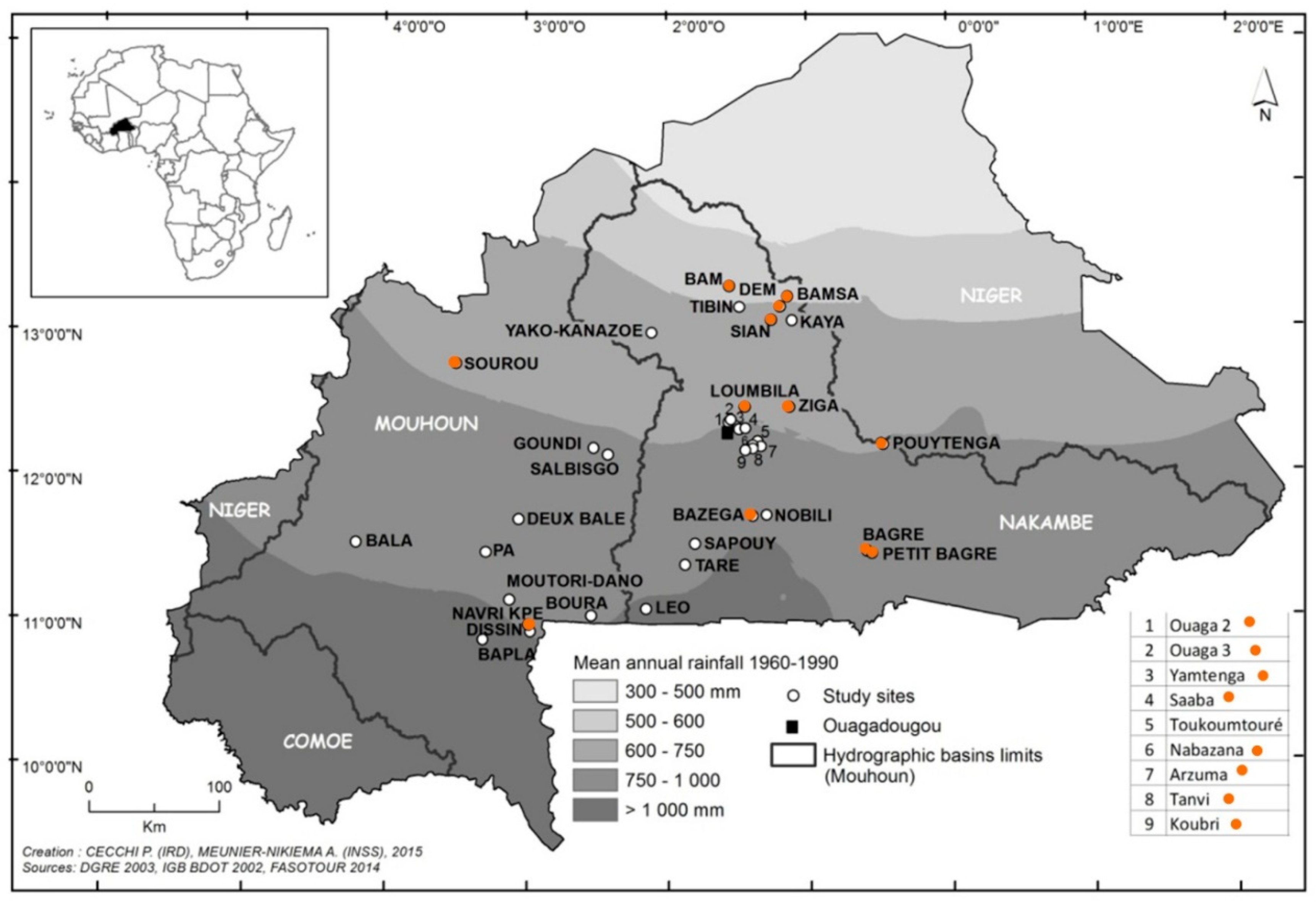
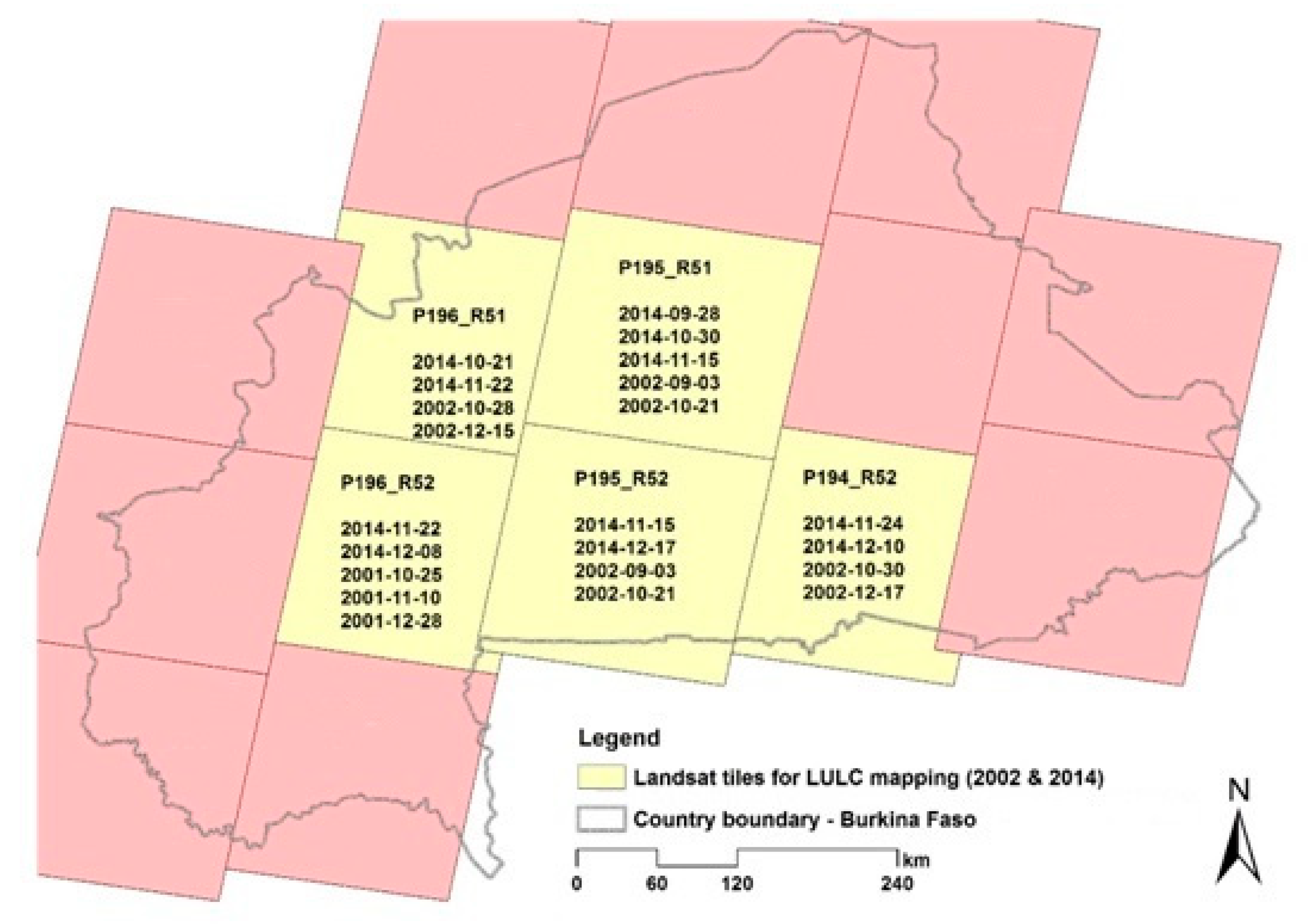
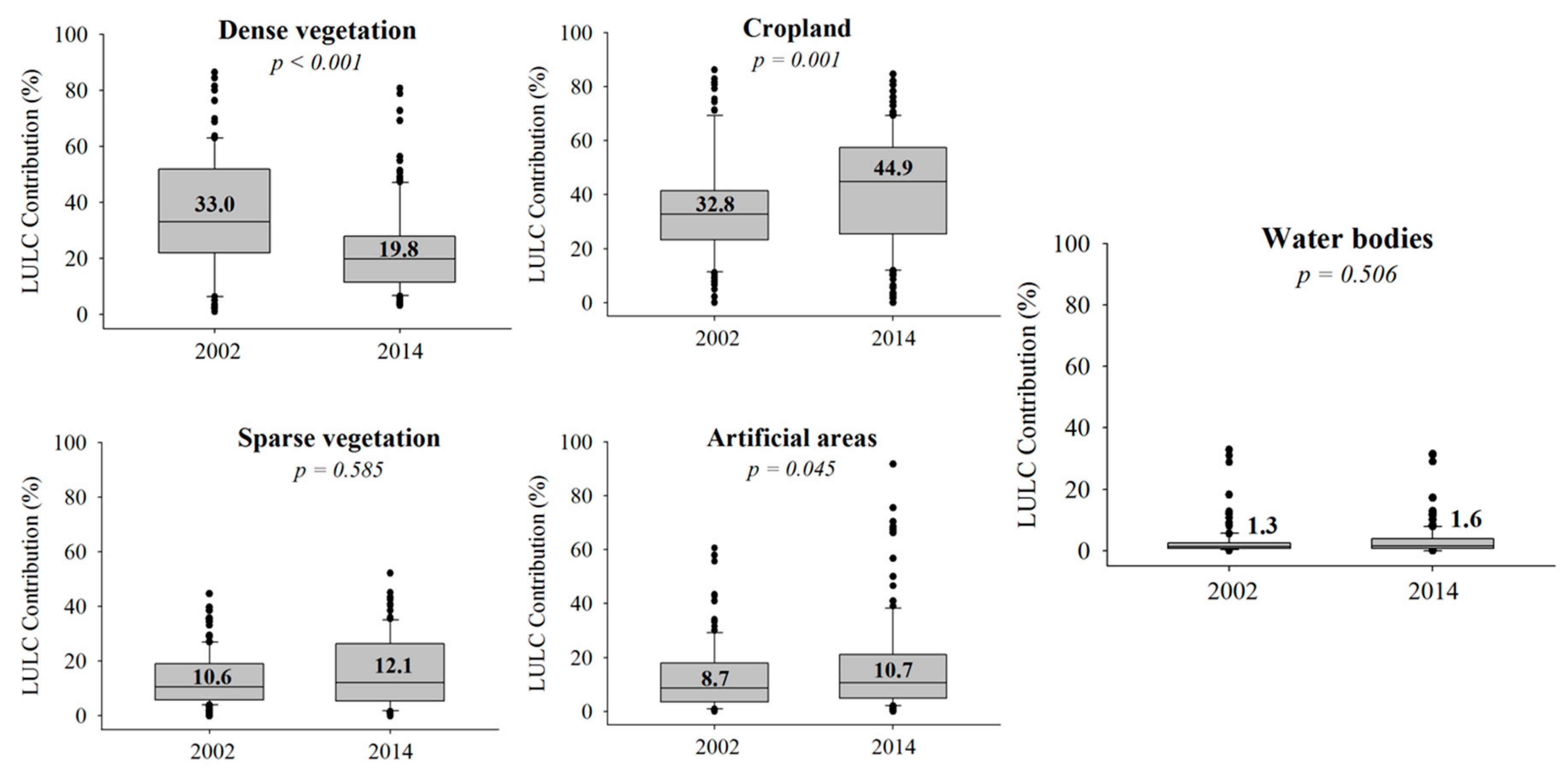
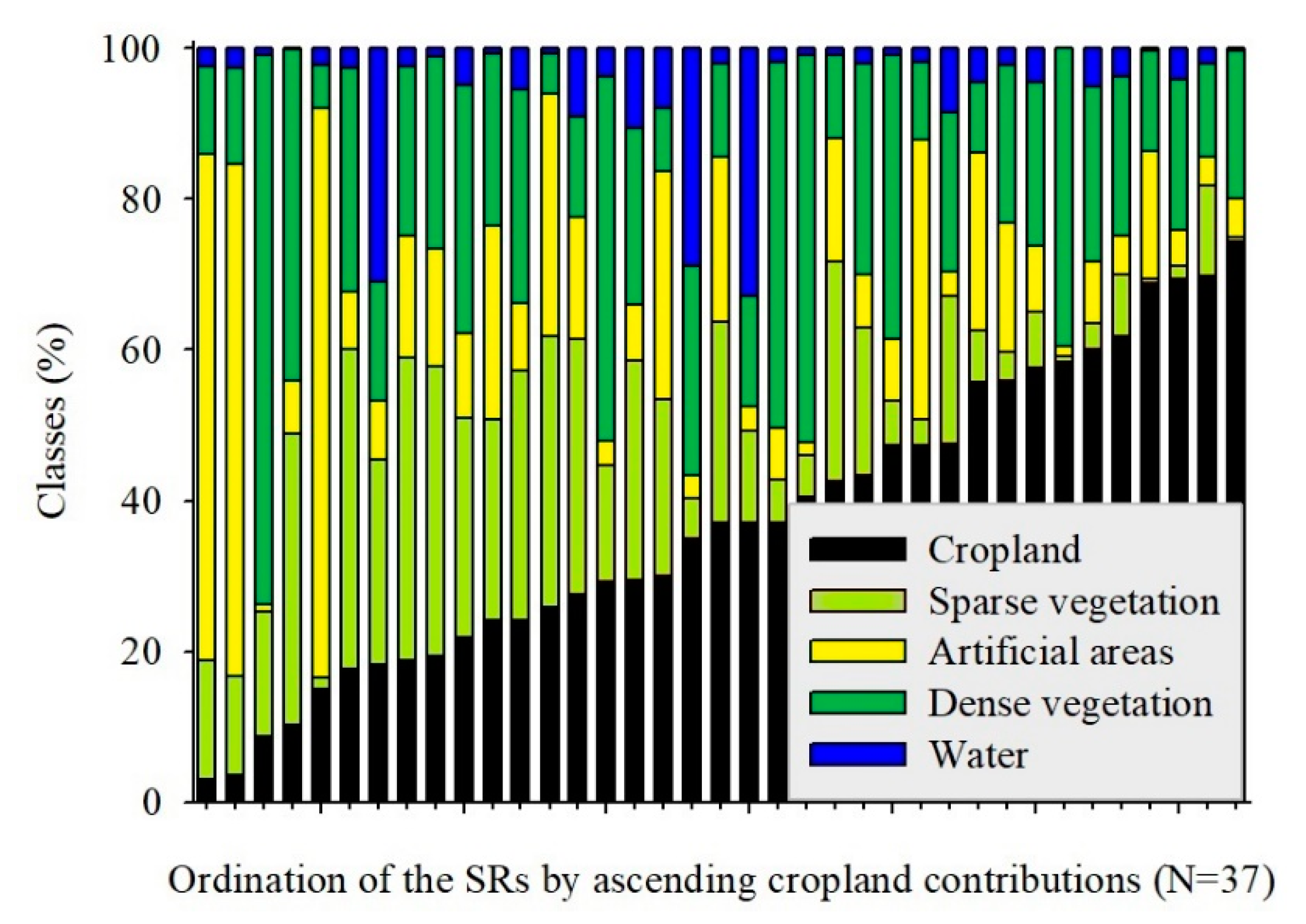
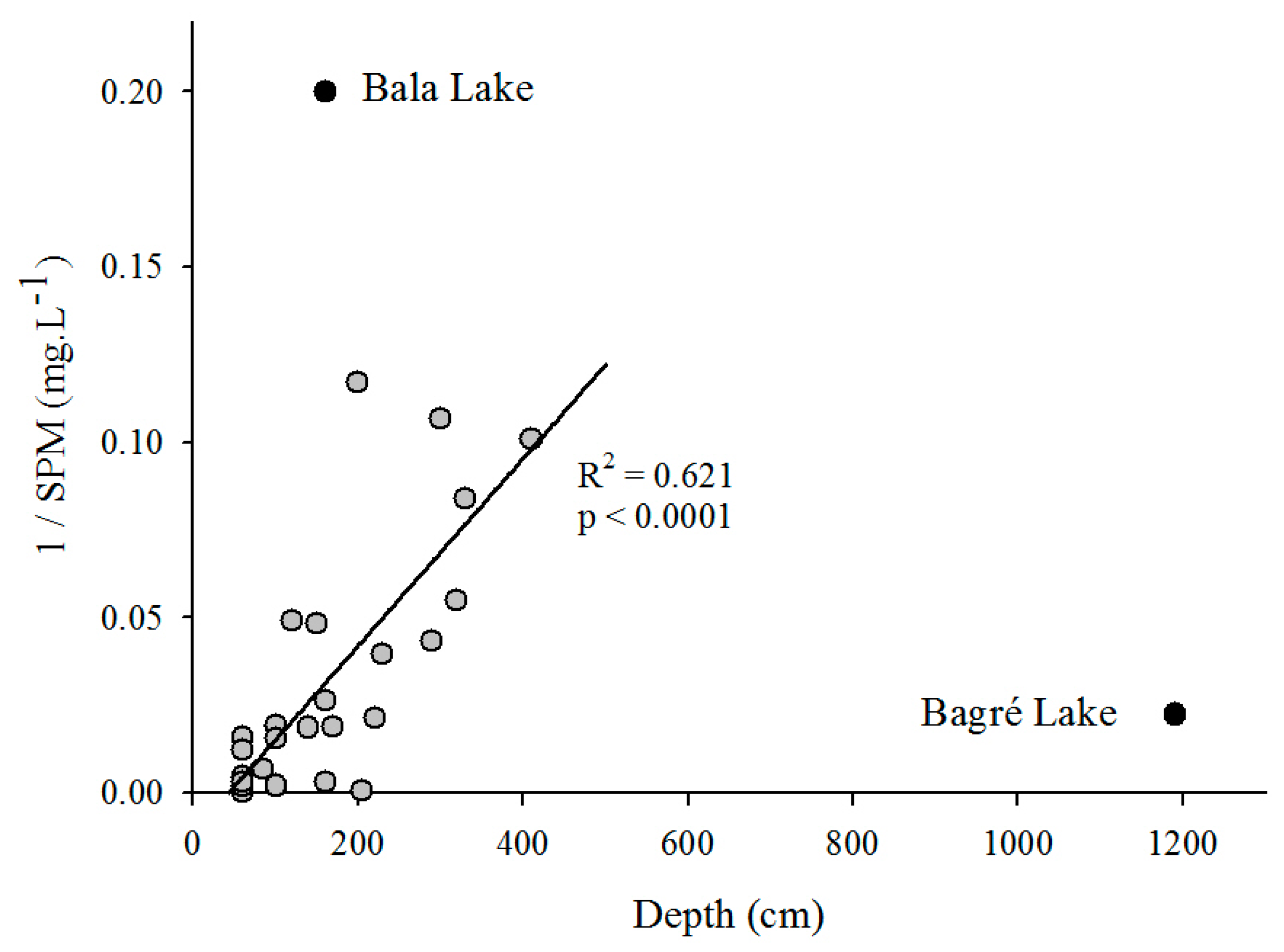
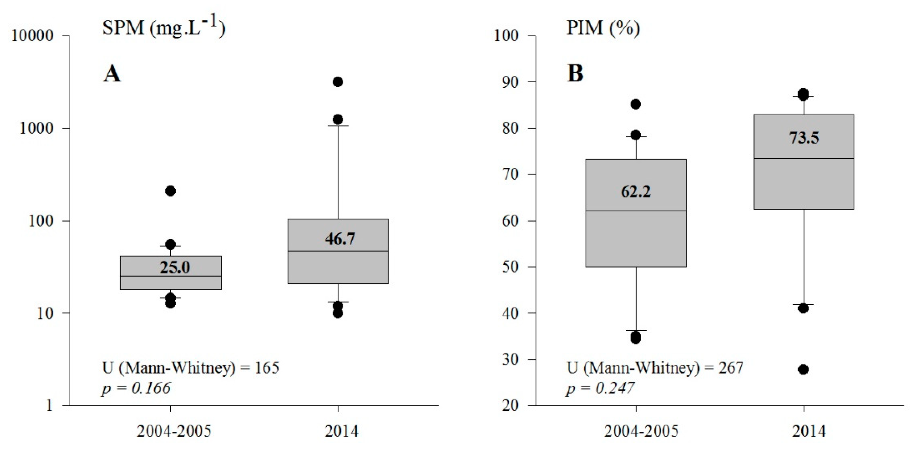
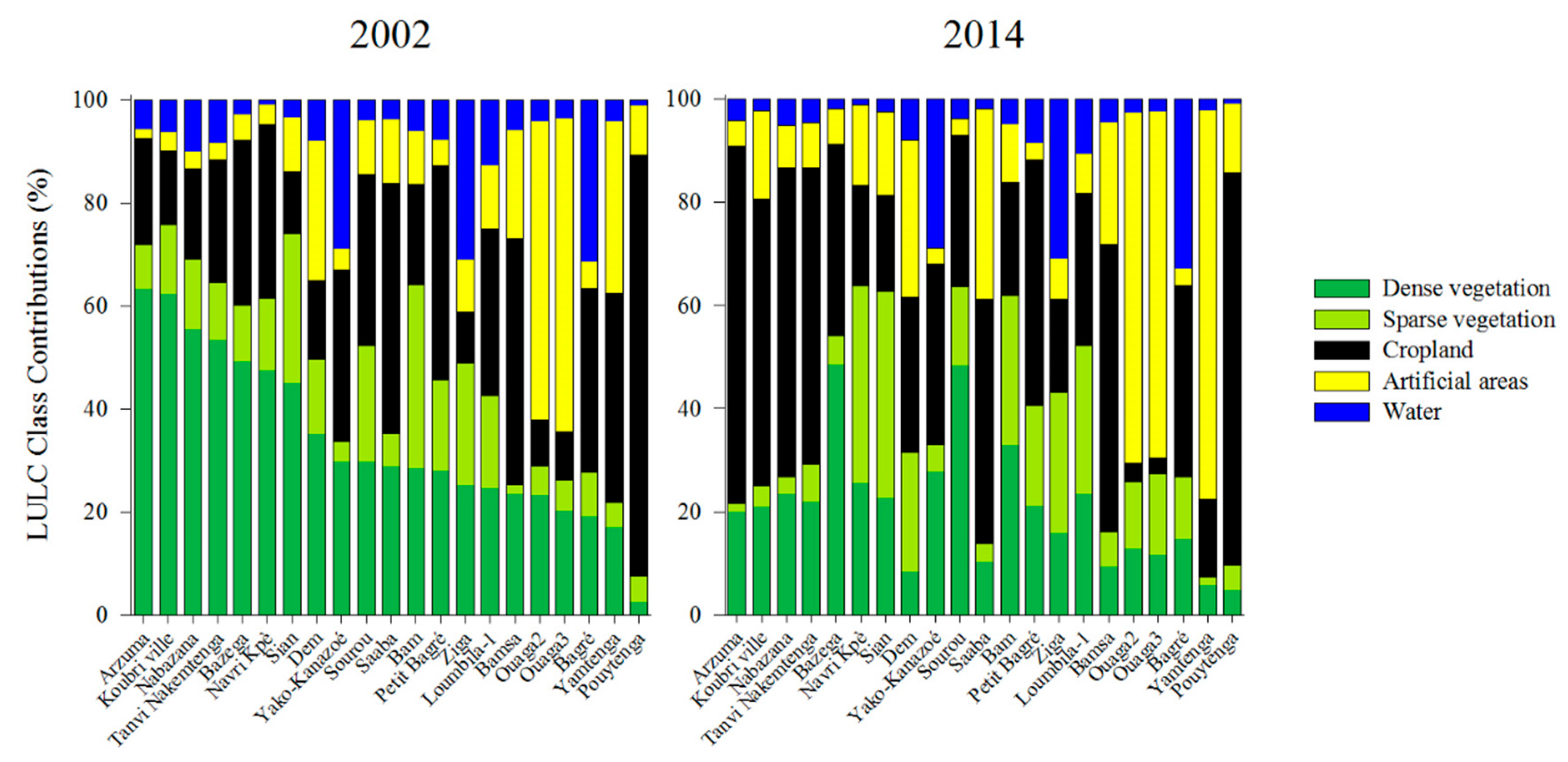
Table 1.
Sites studied in Burkina Faso during the 2014 dry season, ranked by alphabetical order.
| Site | Latitude | Longitude | Depth | dS | pH | C25 | Chl a | SPM | PIM | Capacity | Cropland | Surface | Pop. Density |
|---|---|---|---|---|---|---|---|---|---|---|---|---|---|
| (cm) | (cm) | (i.u.) | (µS·L−1) | (µg·L−1) | (mg·L−1) | (%) | (Mm3) | (%) | (km2) | (Inh·km−2) | |||
| Arzuma | 12°13′07.6″ | 01°17′46.0″ | 150 | 48.0 | 7.8 | 105.3 | 27.1 | 20.7 | 47 | 1.4 | 69.4 | 885 | 141.6 |
| Bagré | 11°29′25.7″ | 00°32′56.9″ | 1190 | 16.0 | 7.5 | 86.6 | 2.6 | 44.7 | 82.5 | 1700.0 | 37.1 | 35,308 | 158.3 |
| Bala | 11°33′37.9″ | 04°09′24.8″ | 160 | 137.0 | 6.6 | 129.6 | 5.3 | 5.0 | 62.9 | 1.5 | 8.7 | 37.3 | 13.7 |
| Bam | 13°19′57.4″ | 01°30′48.8″ | 160 | 19.5 | 7.6 | 101.1 | 10.5 | 38.1 | 81.1 | 31.0 | 21.8 | 2608 | 71.7 |
| Bamsa | 13°15′36.2″ | 01°06′02.8″ | 220 | 23.8 | 7.9 | 115.4 | 12.0 | 46.7 | 74.5 | n.d. | 55.7 | 189 | 52.2 |
| Bapla-Diébougou | 10°52′56.0″ | 03°15′46.7″ | 300 | 90.5 | 8.5 | 257.0 | 23.8 | 9.4 | 28.9 | n.d. | 24.1 | 423 | 40.6 |
| Bazega | 11°44′06.2″ | 01°21′12.0″ | 230 | 36.5 | 7.4 | 94.9 | 44.1 | 25.3 | 41 | 11.2 | 37.1 | 246 | 78 |
| Boura | 11°02′49.3″ | 02°29′52.1″ | 330 | 56.5 | 8.1 | 75.0 | 15.9 | 11.9 | 51.2 | 4.2 | 40.6 | 156 | 16.7 |
| Dem | 13°11′27.8″ | 01°09′12.1″ | 120 | 38.1 | 7.8 | 141.4 | 25.8 | 20.4 | 68.6 | 4.0 | 30.1 | 577 | 65.1 |
| Deux Balé | 11°43′04.9″ | 03°00′37.5″ | n.d. | 26.0 | 7.7 | 132.7 | 42.8 | 26.8 | 42.9 | 6.0 | 17.7 | 1000 | 45.7 |
| Dissin | 10°56′21.7″ | 02°55′36.4″ | 60 | 9.0 | 7.5 | 73.8 | n.m. | 237.9 | 85 | 0.1 | 24.1 | 0.6 | 9282.2 |
| Goundi | 12°12′48.4″ | 02°28′37.1″ | 100 | 11.0 | 8.6 | 106.4 | 17.9 | 53.2 | 77.2 | n.d. | 42.6 | 9.8 | 47.9 |
| Kaya | 13°05′33.4″ | 01°04′07.5″ | n.d. | 11.0 | 8.5 | 230.3 | 25.4 | 391.0 | 84.3 | 1.1 | 25.9 | 9.1 | 368.1 |
| Koubri | 12°11′34.0″ | 01°24′16.2″ | 205 | 1.5 | 5.7 | n.d. | n.m. | 1240.0 | 87 | 9.7 | 55.9 | 449 | 211.8 |
| Leo | 11°05′34.0″ | 02°06′35.4″ | 60 | 7.5 | 6.3 | 114.0 | n.m. | 485.0 | 87.6 | 0.1 | 47.3 | 9.3 | 2308.2 |
| Loumbila | 12°29′34.0″ | 01°24′25.8″ | 330 | 64.7 | 7.6 | n.d. | n.d. | 11.9 | 56.3 | 42.2 | 29.4 | 2079 | 87.1 |
| Moutori-Dano | 11°09′29.7″ | 03°04′32.3″ | 60 | 17.5 | 8.3 | 170.7 | 64.6 | 63.5 | 65.5 | n.d. | 10.3 | 7.8 | 67.3 |
| Nabazana | 12°12′13.4″ | 01°21′07.8″ | 100 | 20.0 | 7.7 | 97.6 | 24.7 | 51.7 | 71 | 4.0 | 60.1 | 679 | 167.2 |
| Navri Kpè | 10°59′05.3″ | 02°56′26.7″ | n.d. | 46.0 | 7.4 | 117.9 | 53.8 | 21.2 | 27.8 | 2.6 | 19.4 | 76.2 | 72 |
| Nobili | 11°44′27.6″ | 01°15′24.0″ | 60 | 7.0 | 7.0 | 97.0 | n.m. | 217.9 | 83.7 | 0.7 | 68.8 | 14 | 78.4 |
| Ouaga2 | 12°23′16.7″ | 01°31′22.4″ | 85 | 10.0 | 7.7 | 309.8 | 64.5 | 144.5 | 73.5 | 1.2 | 3.6 | 310 | 1892.6 |
| Ouaga3 | 12°23′24.9″ | 01°30′29.3″ | 140 | 28.5 | 8.6 | 92.5 | 65.5 | 53.6 | 72 | 1.5 | 2.9 | 369 | 3127.5 |
| Pa | 11°29′23.9″ | 03°14′33.6″ | 200 | 80.5 | 7.7 | 96.4 | 17.4 | 8.6 | 58.4 | n.d. | 69.7 | 246 | 45.9 |
| Petit Bagré | 11°28′25.4″ | 00°30′47.0″ | n.d. | 17.0 | 7.5 | 111.1 | 1.2 | 52.1 | 82.5 | 3.5 | 47.6 | 32.8 | 65.4 |
| Pouytenga | 12°13′41.5″ | 00°25′54.9″ | 60 | 2.5 | 7.4 | 480.9 | n.m. | 3153.3 | 87.5 | 0.6 | 76.1 | 13.4 | 421.4 |
| Saaba | 12°20′39.8″ | 01°24′12.2″ | 60 | n.d. | 7.9 | 369.9 | 66.3 | 333.0 | 84.4 | 5.4 | 47.4 | 141 | 2572.1 |
| Salbisgo | 12°09′53.6″ | 02°22′36.1″ | 100 | 10.0 | 7.7 | 362.8 | 15.8 | 481.3 | 87.5 | 3.6 | 43.4 | 188 | 135.7 |
| Sapouy | 11°32′38.6″ | 01°45′45.8″ | 160 | 7.0 | 6.3 | n.d. | n.m. | 313.2 | 83.9 | 0.7 | 74.4 | 34 | 46.9 |
| Sian | 13°05′46.1″ | 01°13′04.7″ | 100 | 14.7 | 7.8 | 163.3 | 14.3 | 64.7 | 83.5 | 2.0 | 18.7 | 760 | 71 |
| Sourou | 12°48′07.2″ | 03°26′55.9″ | 320 | 57.0 | 8.6 | 226.0 | 33.4 | 18.2 | 45.1 | 370.0 | 29.3 | 30,214 | 21.3 |
| Tanvi Nakemtenga | 12°13′35.7″ | 01°21′06.6″ | 170 | 29.0 | 7.6 | 105.3 | 15.8 | 53.1 | 69.1 | 0.6 | 57.5 | 25 | 54.4 |
| Taré | 11°23′55.7″ | 01°49′55.9″ | 60 | 20.0 | 6.9 | n.d. | 52.2 | 81.5 | 72.9 | n.d. | 58.3 | 4.5 | 40.9 |
| Tibin | 13°11′11.8″ | 01°26′36.0″ | n.d. | n.d. | 7.3 | 138.6 | 15.0 | 167.6 | 89 | 0.0 | 27.5 | 3052 | 72.5 |
| Toukoumtouré | 12°15′17.3″ | 01°19′02.6″ | 60 | 4.5 | 6.7 | 75.1 | n.m. | 580.0 | 85.3 | 0.4 | 61.8 | 12.1 | 58.4 |
| Yako-Kanazoé | 13°00′41.9″ | 02°03′55.1″ | 410 | 79.0 | 7.6 | 136.1 | 11.7 | 9.9 | 71.2 | 75.0 | 35 | 8127 | 105.6 |
| Yamtenga | 12°20′20.1″ | 01°26′51.0″ | 60 | 9.0 | 7.9 | 350.0 | n.m. | 319.0 | 86.2 | 0.6 | 15.1 | 12.2 | 5256.3 |
| Ziga | 12°29′24.4″ | 01°05′25.5″ | 290 | 35.0 | 7.4 | 112.3 | 9.0 | 23.0 | 77.6 | 200.0 | 18.2 | 20,689 | 97.8 |
Depth: measured at the sampling station; dS: Secchi disk disappearance depth; pH: sub-surface pH value; C25: equivalent conductivity at 25 °C; Chl a: sub-surface chlorophyll a concentration; SPM: Suspended Particulate Matter; PIM: Particulate Inorganic Matter; Capacity: storage capacity of the water body; Cropland: cropland class contribution within 5-km radius buffer area around reservoirs in 2014; Surface: the surface of the watershed; Pop. Density: 2014 population density at the watershed scale. n.d.: non-determined values; n.m.: non-measurable Chl a values owing to excessive turbidity.
Table 2.
Spearman rank–order correlation coefficients between 2014 LULC classes at different scales around SRs (n = 37). Associated probabilities are indicated in italics and significant statistics in bold.
Table 2.
Spearman rank–order correlation coefficients between 2014 LULC classes at different scales around SRs (n = 37). Associated probabilities are indicated in italics and significant statistics in bold.
| 5-km Buffer | Sparse vegetation | Dense vegetation | Water | Artificial areas |
| Cropland | −0.648 (<0.001) | −0.228 (0.151) | −0.142 (0.374) | −0.281(0.075) |
| Sparse vegetation | 0.131(0.413) | 0.223 (0.160) | 0.112 (0.486) | |
| Dense vegetation | −0.058 (0.717) | −0.594 (<0.001) | ||
| Water | −0.098 (0.541) | |||
| Watershed | Sparse vegetation | Dense vegetation | Water | Artificial areas |
| Cropland | −0.354 (0.023) | −0.164 (0.302) | 0.112 (0.484) | −0.259 (0.102) |
| Sparse vegetation | 0.152 (0.341) | 0.143 (0.370) | −0.160 (0.317) | |
| Dense vegetation | −0.476 (0.002) | −0.672 (<0.001) | ||
| Water | 0.192 (0.227) |
Table 3.
Autocorrelations of anthropogenic pressures’ proxies around SRs (n = 37). Statistically significant (p < 0.01) Spearman rank–order correlation coefficients and their associated probabilities are indicated in bold and italics, respectively.
Table 3.
Autocorrelations of anthropogenic pressures’ proxies around SRs (n = 37). Statistically significant (p < 0.01) Spearman rank–order correlation coefficients and their associated probabilities are indicated in bold and italics, respectively.
| Watershed | |||||||
|---|---|---|---|---|---|---|---|
| Population Density | Cropland | Sparse Vegetation | Dense Vegetation | Water | Artificial Areas | ||
| Watershed | Population Density | −0.070 | −0.324 | −0.465 | 0.071 | 0.601 | |
| 0.664 | 0.039 | 0.002 | 0.655 | <0.001 | |||
| 5-km Buffer area | Cropland | −0.015 | 0.667 | −0.340 | 0.009 | 0.051 | −0.259 |
| 0.927 | <0.001 | 0.030 | 0.956 | 0.751 | 0.101 | ||
| Sparse vegetation | −0.220 | −0.323 | 0.747 | 0.030 | 0.212 | −0.046 | |
| 0.165 | 0.040 | <0.001 | 0.853 | 0.182 | 0.775 | ||
| Dense vegetation | −0.447 | −0.135 | 0.065 | 0.742 | −0.528 | −0.469 | |
| 0.004 | 0.399 | 0.687 | <0.001 | <0.001 | 0.002 | ||
| Water | −0.033 | 0.173 | 0.238 | −0.001 | 0.212 | 0.042 | |
| 0.836 | 0.277 | 0.134 | 0.995 | 0.182 | 0.793 | ||
| Artificial areas | 0.540 | −0.264 | −0.059 | −0.676 | 0.304 | 0.788 | |
| <0.001 | 0.095 | 0.714 | <0.001 | 0.053 | <0.001 | ||
Table 4.
Non-parametric Spearman rank–order correlation coefficients and associated probabilities (italics), between Suspended Particulate Matter (SPM) and Particulate Inorganic Matter (PIM) values, and environmental variables.
Table 4.
Non-parametric Spearman rank–order correlation coefficients and associated probabilities (italics), between Suspended Particulate Matter (SPM) and Particulate Inorganic Matter (PIM) values, and environmental variables.
| PIM (%) | Depth (cm) | dS (cm) | pH (i.u.) | C25 (µS·cm−1) | Chl a (µg·L−1) | Cropland (%) | Surface (km2) | Pop. Density (Inh·km−2) | Capacity (Mm3) | |
|---|---|---|---|---|---|---|---|---|---|---|
| SPM | 0.846 | −0.723 | −0.950 | −0.245 | 0.216 | 0.245 | 0.238 | −0.524 | 0.534 | −0.569 |
| (mg·L−1) | <0.001 | <0.001 | <0.001 | 0.143 | 0.225 | 0.207 | 0.157 | <0.001 | <0.001 | <0.001 |
| PIM | −0.555 | −0.864 | −0.325 | 0.160 | −0.354 | 0.219 | −0.303 | 0.523 | −0.513 | |
| (%) | <0.001 | <0.001 | 0.050 | 0.370 | 0.064 | 0.191 | 0.068 | <0.001 | 0.003 | |
| Depth | 0.649 | 0.096 | −0.231 | −0.559 | −0.127 | 0.724 | −0.374 | 0.773 | ||
| (cm) | <0.001 | 0.598 | 0.234 | 0.006 | 0.485 | <0.001 | 0.035 | <0.001 | ||
| dS | 0.323 | −0.065 | −0.016 | −0.258 | 0.474 | −0.490 | 0.558 | |||
| (cm) | 0.058 | 0.725 | 0.936 | 0.134 | 0.004 | 0.003 | 0.002 | |||
| pH | 0.280 | 0.385 | −0.314 | 0.099 | −0.027 | 0.187 | ||||
| (i.u.) | 0.113 | 0.043 | 0.058 | 0.557 | 0.874 | 0.319 | ||||
| C25 | 0.261 | −0.238 | −0.003 | 0.109 | 0.009 | |||||
| (µS·cm−1) | 0.187 | 0.181 | 0.987 | 0.545 | 0.960 | |||||
| Chl a | −0.137 | −0.271 | 0.217 | −0.201 | ||||||
| (µg·L−1) | 0.482 | 0.161 | 0.264 | 0.376 | ||||||
| Cropland | −0.201 | −0.091 | −0.144 | |||||||
| (%) | 0.231 | 0.591 | 0.435 | |||||||
| Surface | −0.056 | 0.737 | ||||||||
| (km2) | 0.740 | <0.001 | ||||||||
| Pop. Density | −0.206 | |||||||||
| (Inh·km−2) | 0.264 |
(SPM: Suspended Particulate Matter; PIM: Particulate Inorganic Matter; Depth: measured depth at the sampling station; dS: Secchi disk disappearance depth; pH: sub-surface pH value; C25: equivalent conductivity at 25 °C; Chl a: sub-surface chlorophyll a concentration; Cropland: cropland class contribution within 5-km radius buffer areas around reservoirs; Surface: surface of watersheds; Pop. Density: population density at the watershed scale; Capacity: volume of studied water masses). Statistically significant results are in bold.
Table 5.
Non-parametric Spearman rank–order correlation coefficients and associated probabilities (italics), between rates of change (2002–2014), of SPM load [Δ (SPM)], PIM contribution [Δ (PIM)], and LULC classes’ contribution within 5-km buffer areas around water masses [Δ (Crop areas), Δ (Sparse vegetation), etc.]. Statistically significant results are in bold.
| Δ (PIM) | Δ (Crop Areas) | Δ (Sparse Vegetation) | Δ (Dense Vegetation) | Δ (Water Bodies) | Δ (Artificial Areas) | |
|---|---|---|---|---|---|---|
| Δ (SPM) | 0.248 | −0.240 | −0.330 | −0.071 | −0.521 | 0.457 |
| 0.274 | 0.289 | 0.141 | 0.754 | 0.016 | 0.037 | |
| Δ (PIM) | 0.579 | −0.419 | −0.317 | −0.360 | 0.274 | |
| 0.006 | 0.058 | 0.159 | 0.107 | 0.225 | ||
| Δ (Crop areas) | −0.438 | −0.418 | −0.181 | 0.310 | ||
| 0.047 | 0.058 | 0.428 | 0.168 | |||
| Δ (Sparse vegetation) | 0.171 | 0.514 | −0.400 | |||
| 0.452 | 0.017 | 0.071 | ||||
| Δ (Dense vegetation) | 0.436 | −0.647 | ||||
| 0.047 | 0.002 | |||||
| Δ (Water bodies) | −0.610 | |||||
| 0.003 |
© 2020 by the authors. Licensee MDPI, Basel, Switzerland. This article is an open access article distributed under the terms and conditions of the Creative Commons Attribution (CC BY) license (http://creativecommons.org/licenses/by/4.0/).
Share and Cite
MDPI and ACS Style
Cecchi, P.; Forkuor, G.; Cofie, O.; Lalanne, F.; Poussin, J.-C.; Jamin, J.-Y. Small Reservoirs, Landscape Changes and Water Quality in Sub-Saharan West Africa. Water 2020, 12, 1967. https://doi.org/10.3390/w12071967
AMA Style
Cecchi P, Forkuor G, Cofie O, Lalanne F, Poussin J-C, Jamin J-Y. Small Reservoirs, Landscape Changes and Water Quality in Sub-Saharan West Africa. Water. 2020; 12(7):1967. https://doi.org/10.3390/w12071967
Chicago/Turabian StyleCecchi, Philippe, Gerald Forkuor, Olufunke Cofie, Franck Lalanne, Jean-Christophe Poussin, and Jean-Yves Jamin. 2020. "Small Reservoirs, Landscape Changes and Water Quality in Sub-Saharan West Africa" Water 12, no. 7: 1967. https://doi.org/10.3390/w12071967
Note that from the first issue of 2016, this journal uses article numbers instead of page numbers. See further details here.