Toward a Harmonization for Using in situ Nutrient Sensors in the Marine Environment
 Anne Daniel1*
  Agathe Laës-Huon2
  Carole Barus3
  Alexander D. Beaton4
  Daniel Blandfort5
  Nathalie Guigues6
  Marc Knockaert7 Dominique Munaron8
  Ian Salter9,10
  E. Malcolm S. Woodward11
  Naomi Greenwood12
  Eric P. Achterberg13
- 1Laboratoire Ecologie Pélagique, Unité Dynamiques des Écosystèmes Côtiers, Ifremer, Plouzané, France
- 2Laboratoire Détection, Capteurs et Mesures, Unité Recherches et Développements Technologiques, Ifremer, Plouzané, France
- 3Laboratoire d’Etudes en Géophysique et Océanographie Spatiales, UMR 5566, CNRS/UPS/CNES/IRD, Toulouse, France
- 4Ocean Technology and Engineering Group, National Oceanography Centre, Southampton, United Kingdom
- 5Institut für Küstenforschung, Helmholtz-Zentrum Geesthacht, Geesthacht, Germany
- 6Pôle Chimie et Biologie, Direction de la Métrologie Scientifique et Industrielle, LNE, Paris, France
- 7ECOCHEM, Operationele Directie Natuurlijk Milieu, Ostend, Belgium
- 8MARBEC, Ifremer, IRD, Univ. Montpellier, CNRS, Sète, France
- 9Faroe Marine Research Institute, Tórshavn, Faroe Islands
- 10Helmholtz Centre for Polar and Marine Research, Alfred Wegener Institute, Bremerhaven, Germany
- 11Plymouth Marine Laboratory, Plymouth, United Kingdom
- 12Centre for Environment, Fisheries and Aquaculture Science, Lowestoft, United Kingdom
- 13GEOMAR, Helmholtz Centre for Ocean Research, Kiel, Germany
Improved comparability of nutrient concentrations in seawater is required to enhance the quality and utility of measurements reported to global databases. Significant progress has been made over recent decades in improving the analysis and data quality for traditional laboratory measurements of nutrients. Similar efforts are required to establish high-quality data outputs from in situ nutrient sensors, which are rapidly becoming integral components of ocean observing systems. This paper suggests using the good practices routine established for laboratory reference methods to propose a harmonized set of deployment protocols and of quality control procedures for nutrient measurements obtained from in situ sensors. These procedures are intended to establish a framework to standardize the technical and analytical controls carried out on the three main types of in situ nutrient sensors currently available (wet chemical analyzers, ultraviolet optical sensors, electrochemical sensors) for their deployments on all kinds of platform. The routine reference controls that can be applied to the sensors are listed for each step of sensor use: initial qualification under controlled conditions in the laboratory, preparation of the sensor before deployment, field deployment and finally the sensor recovery. The fundamental principles applied to the laboratory reference method are then reviewed in terms of the calibration protocol, instrumental interferences, environmental interferences, external controls, and method performance assessment. Data corrections (linearity, sensitivity, drifts, interferences and outliers) are finally identified along with the concepts and calculations for qualification for both real time and time delayed data. This paper emphasizes the necessity of future collaborations between research groups, reference-accredited laboratories, and technology developers, to maintain comparability of the concentrations reported for the various nutrient parameters measured by in situ sensors.
Introduction
Nutrients are identified by the GOOS expert panels as one of the EOVs1. The measurement of nutrient concentrations in seawater provides a number of challenges, which are specific to the marine system. Strong concentration gradients are typically observed from estuarine, coastal and open ocean waters (Zhang et al., 2007). Vertical concentration gradients also occur as a result of processes including biological uptake, remineralization of sinking organic particles and upwelling of nutrient-rich deep waters into the euphotic zone (Sigman and Hain, 2012). In addition to better resolved spatial data, high temporal resolution measurements are required to characterize daily or semi-diurnal processes including episodic and transient events (phytoplankton blooms, storms, runoff, waste water treatment discharges, etc…). Furthermore, nutrient changes driven by natural and anthropogenic global change are only fully understandable by applying long-term observations integrated over months to years (Evans et al., 2003).
The sampling and analysis of seawater samples for nutrient determination is traditionally carried out by taking discrete water samples using a dedicated water sampling device. Subsequent analysis can be conducted either on board survey vessels or in a land-based laboratory using a variety of analytical instruments. It is apparent that in certain cases traditional sampling and analysis approaches are insufficient to resolve correctly episodic events or local phenomena (Prien, 2007). In situ nutrient sensors have thus been identified as critical tools across the marine biogeochemical and biological communities to enhance the spatial and temporal resolution of nutrient profiles to be able to investigate these events in finer detail.
However, nutrients have historically been more difficult to measure in situ than physical parameters such as salinity and temperature. Instrumentation for in situ measurement of nutrients in seawater first appeared in the late 1980s (Johnson et al., 1986, 1989). Over the last 30 years, manufacturers and research institutions have attempted to develop more compact devices that are simpler to operate, with lower power and reagent consumption and requiring less maintenance. Various detection technologies have been employed including spectrophotometry, fluorometry and electrochemistry. Despite significant technological progress numerous challenges remain in the correct application of instrumentation to guarantee comparability of data from different analytical systems. These challenges include:
– level of reliability a priori lower than for reference laboratory techniques,
– lack of harmonized deployment protocols,
– limit of detection insufficient to quantify nutrient concentrations in some research areas (e.g., oligotrophic waters),
– difficulties in interpreting results following completion of metrology operations (e.g., calibration) of pre- and post-deployment as a result (e.g., sensor drift, biofouling),
– absence of quality control procedures and standards to validate and certify in situ data.
Nowadays, it is fundamental to be able to compare nutrient data from all technologies with full confidence in order to be able to report the values to global data bases. Standardized approaches to in situ nutrient measurements are an essential condition for effective global monitoring of the ocean. As a result of the work by the oceanographic community over more than 60 years, it is now crucial that nutrient sensors benefit from the experience and best practices that have been established for standard laboratory methods.
The AtlantOS2 and JERICO3 European projects organized a joint workshop focusing on the “interoperability of technologies and best practices – in situ applications to nutrient measurements” in December 2018. This workshop highlighted a disparity in the way in which users control the deployment of sensors and in which raw data from sensors are processed. This working group proposes to build upon quality control procedures that have been implemented for standard laboratory methods, and to use essential parts of these procedures for the qualification of in situ nutrient data sets. After reviewing the existing techniques to measure nutrients in seawater, we provide here a set of quality procedures for field measurements along with concepts and calculations for data qualification. The goal is to propose a protocol that can be easily used and adopted by end-users, and standardized between different technology types.
Review of Existing Techniques to Measure Nutrients in Seawater
The main macro-nutrient elements playing a major role in stimulating planktonic primary production in the oceans and, regulating the amount of organic carbon fixed by phytoplankton, are nitrogen and phosphorus. A third important macro-nutrient is silicon because of its uptake by diatoms, a major class of single-cell algae with a silicaceous skeleton. The commonly designated nutrients are dissolved inorganic nitrogen compounds (three main forms: nitrate NO3–, nitrite NO2– and ammonium NH4+), dissolved inorganic phosphorus (under the pre-dominant form orthophosphate PO43–, analytically defined as Soluble Reactive Phosphate), and the dissolved forms of the orthosilicate ion (commonly known as silicate, the predominant form being orthosilicic acid Si(OH)4). The abundance of nutrients determines how productive the waters are. Nutrient ratios also provide useful chemical signatures to distinguish oceanic water masses and identify their origins.
Laboratory Benchmark Techniques for Nutrient Analysis in Seawater
A variety of methods has been established since the 1950s to determine nutrients in seawater. The first category of methods includes the manual methods where each sample is treated individually. A second category of methods is composed of automated methods based on flow analysis: a peristaltic pump delivers sample and reagents into tubing and mixing coils which acts as the reaction vessel before the flow stream reaches a detector. Two main techniques of flow analysis are used to measure nutrients: FIA and SFA. FIA (Růžička and Hansen, 1981) is the injection of a sample into a moving continuous carrier stream of reagent. The reaction zone is then transported toward the detector that continuously records the changes in absorbance within the flow cell. SFA is a continuous flow divided by air bubbles into discrete segments to minimize dispersion and enhance the mixing with reagents. FIA is not as sensitive or precise as SFA because detection occurs in a transition phase. SFA is the analytical system most widely used by marine chemists and has become the unofficial benchmark technique as it offers simplicity of operation, rapid sample throughput and outstanding analytical performance. Since the mid-1970s, most oceanographic laboratories have been using SFA AutoAnalysers commercialized by Technicon.
Due to the significance of nutrient measurements in marine systems, they are among the most commonly analyzed parameters in oceanographic research. Since the publication of the first well known seawater nutrient analysis handbooks (Strickland and Parsons, 1972; Grasshoff, 1976), numerous comprehensive methods and reviews have been published (Miró et al., 2003; Motomizu and Li, 2005; Gray et al., 2006; Molins-Legua et al., 2006; Aminot and Kérouel, 2007; Aminot et al., 2009; Ma et al., 2016; Worsfold et al., 2016). The first guide suggesting best practice in performing nutrient measurements at sea was proposed by the WOCE in the early 1990s (Gordon et al., 1993). This guide was updated by the GO-SHIP nutrient manual published by Hydes et al. (2010), itself recently rewritten and updated (Becker et al., 2019) as an output of the SCOR International Nutrient Working Group #147. Over the last decade, another important milestone in the quality control of nutrient measurements has been the development and application of CRMs for nutrients. A range of CRMs are now available, which, when used and applied correctly, are starting to improve the quality of nutrient analysis in laboratories and allows for the determination of analytical measurement uncertainty (Aoyama et al., 2018; Birchill et al., 2019).
In situ Nutrient Sensors and Their Deployment Platforms
Ideally, in situ instruments should allow the measurement of short-term variability and also long-term trends, and potentially over a wide global region from the coast to the open ocean. Rarely is a single sensor type suitable for all deployment purposes, applications, platforms or monitoring strategies (Figure 1), but there are sensors whose characteristics are specific to a particular type of deployment. The choice of an in situ nutrient device must be made ensuring that its analytical performance meets the monitoring objectives and taking into account the specific environmental factors of the study area. The expected analytical performance, the deployment platform (e.g., moored/buoy systems, CTD rosette frames, profiling floats, gliders, powered AUVs, benthic chambers, FerryBox-systems) and the characteristics of the water to be measured (expected concentration range and variability, salinity and depth range, temperature variations, presence of potential interferences such as suspended matter) must be identified and taken into account when making the sensor choice. Weight, size, buoyancy, power requirements and communication bandwidth limitations on deployment platforms (Table 1) are also important considerations for data collection and transmission. Furthermore, it must be noted that the optimal benefit-cost ratio forms an important consideration (Griffiths et al., 2001) and actually may be a major limiting factor, especially for expendable platforms such as drifters.
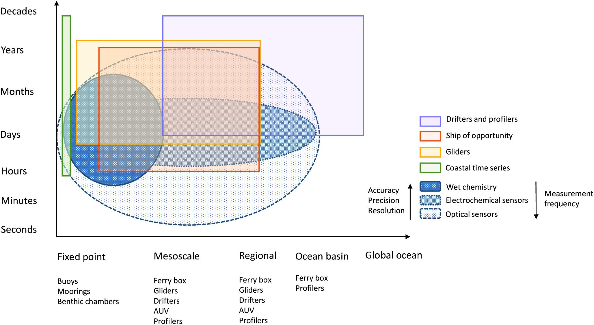
Figure 1. Spatial and temporal coverage of various observing platforms and in situ nutrient sensors (adapted from Liblik et al., 2016).
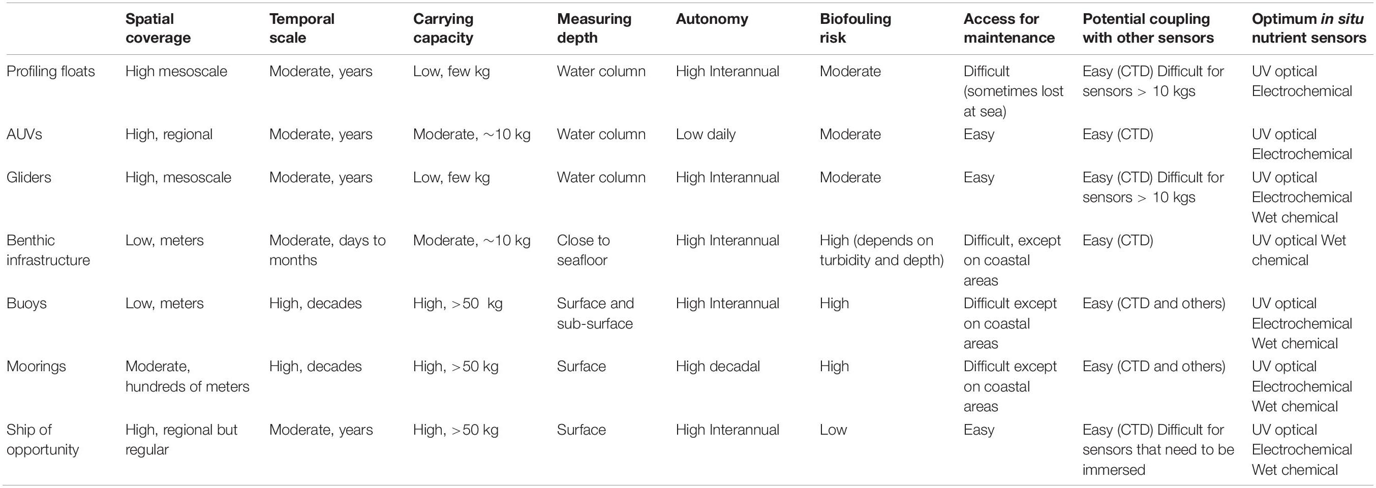
Table 1. Technical constraints of the different types of deployment platforms for the installation of in situ nutrient sensors.
Only dissolved inorganic nutrients can currently be measured by in situ sensors, dedicated instrumentation for the analysis of dissolved organic and particulate nutrients have not yet been developed. In addition to analytical performance, in situ devices have further requirements relative to laboratory techniques, including: physical robustness, resistance to biofouling, high pressure and temperature variations, and stable long-term operation with low energy and, where relevant, low reagent consumption (Mukhopadhyay and Mason, 2013). At present, three main analytical technologies have been used for in situ nutrient monitoring: wet chemical, optical systems, and electrochemistry. While most in situ nutrient sensors are academic prototypes, a list of the commercially available nutrient sensors is available in the ACT database4. Here we attempt to highlight some of the advantages and disadvantages of these three technologies based on independent user experience (Table 2).
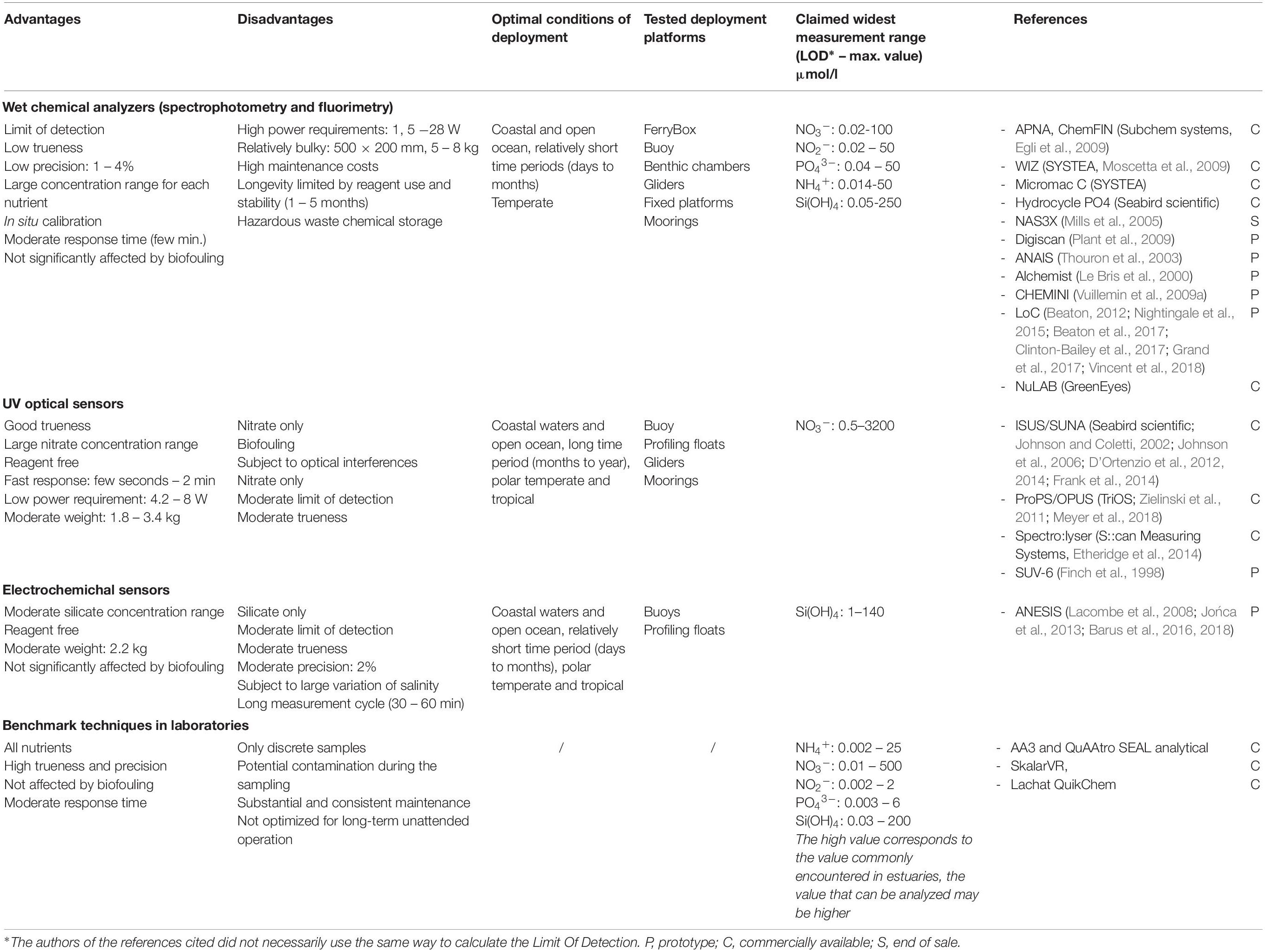
Table 2. Advantages and disadvantages of the analytical technologies used for the in situ determination of nutrients in seawater.
Wet Chemical Analyzers
The basic analytical principles for most of the in situ wet chemical analyzers are derived from standard colorimetric analytical methods, which use chemicals either to form a colored reaction product which is then detected spectroscopically, or by using a fluorescence analytical technique. These in situ analytical instruments are usually based on FIA or on batch analysis. Many instruments based on FIA (Table 2) have been developed and used by academic institutions (Alchimist, Le Bris et al., 2000; NAS3X, Mills et al., 2005; Digiscan, Plant et al., 2009; CHEMINI, Vuillemin et al., 2009a), or are commercially available (APNA/ChemFIN, SubChem Systems Inc.; Hydrocycle, Seabird Scientific). Other devices are based on different flow analysis techniques such as μLFR which is used on WIZ (Systea, Azzaro and Galetta, 2006), or RFA as used on ANAIS (Thouron et al., 2003). Miniaturization of the manifold sensors has been a focus over recent years with the development of sensors based on microfluidics such as LoC devices (Beaton et al., 2011, 2017; Beaton, 2012; Grand et al., 2017). Most wet chemistry systems are recalibrated in situ at regular intervals by replacing the sample by a blank and a standard. Typically, wet chemical analyzers show high resolution, accuracy and precision with a moderate response time (Table 2). The systems are limited by reagent and power consumption, cost, size, and weight (Grand et al., 2019).
Wet chemical analyzers have traditionally been deployed on observing platforms that afford a large load capacity. However, wet chemical analyzers may not always be suitable for long-term deployment due to limited lifetime of reagents and standards and waste disposal concerns. Most wet chemical sensors have been deployed on platforms for the collection of high-frequency time-series of surface coastal waters at a fixed station (NAS3X, Mills et al., 2005; CHEMINI, Répécaud et al., 2009; WIZ, Vuillemin et al., 2009b; LoC, Beaton et al., 2017; Clinton-Bailey et al., 2017; Grand et al., 2017). FerryBox-systems (Petersen et al., 2011) also provide a compatible observing infrastructure for wet chemical analyzers to collect surface nutrient data on board Ships of Opportunity. Wet chemical analyzers have also been deployed as components of benthic incubation chambers (NH4-Digiscan, Plant et al., 2009), and seabed landers, in order to detect nutrient concentration at the water/sediment interface which can vary on hourly to seasonal time scales (Gevaert et al., 2011). Despite their high bulk density, in situ nutrient chemical analyzers have been adapted to moving platforms such as AUVs, to process water column depth profiles (LoC, Vincent et al., 2018), and on ROV’s to characterize the chemical gradients in the patchy distribution of hydrothermal fauna (Alchimist, Le Bris et al., 2000).
Ultraviolet Optical Sensors
The UV optical sensors are chemical-free because they are based on the UV absorption characteristics of seawater constituents. Currently nitrate is the only macronutrient that can be quantified using optical measurement principals. A broad spectral range is required to accurately resolve absorption spectra in complex media such as seawater as the detection of nitrate is based on deconvolution of absorbance spectra that include halogenates such as bromide (Johnson and Coletti, 2002; Frank et al., 2014; Sakamoto et al., 2017). Several commercially available instruments and one prototype can be found: ISUS/SUNA (Seabird Scientific), ProPS/OPUS (TRIOS), Spectro::lyser (S::can Measuring Systems) and SUV-6 (Finch et al., 1998; Pidcock et al., 2010). UV sensors are characterized by a wide concentration range, rapid response times, small size and low power consumption, enabling their deployment across both fixed and profiling observing platforms (Table 2). However, their sensitivity and accuracy are poorer than those of wet chemical analyzers due to a range of optical interferences (dissolved and particulate organic matter). Temperature and salinity compensation, and turbidity correction are required to enhance the analytical performances of the UV optical sensors. Signal drift due to biofouling on the optical measuring window has been observed especially in coastal waters over long deployments (Prien, 2007; Pellerin et al., 2013).
UV optical sensors have been widely used on coastal platforms (Spectro::lyser, Etheridge et al., 2014), moorings (OPUS and SUNA; Collins et al., 2013; Sakamoto et al., 2017) and FerryBox-systems (ProPS, Petersen et al., 2011; SUNA, Frank et al., 2014). Recently Meyer et al. (2018) demonstrated that an in situ UV sensor (OPUS) has the capability to resolve vertical nitrate profiles with high frequency. Three-dimensional profiling platforms, such as BioGeoChemical Argo profiling floats (D’Ortenzio et al., 2012, 2014; Johnson et al., 2017), gliders (Jones et al., 2011), powered AUVs (Johnson and Needoba, 2008) and towed vehicles (Pidcock et al., 2010) have been deployed with UV optical sensors.
Electrochemical Sensors
Electrochemistry proposes promising reagentless sensors that could facilitate miniaturization and decrease energy requirements (Lacombe et al., 2008). Electrochemical methods have been developed to detect silicate (Barus et al., 2016, 2018) and phosphate (Jońca et al., 2011, 2013) in seawater. As silicate and phosphate are non-electroactive compounds, a chemical reaction with molybdates under acidic pH is required to transform these nutrients into silico- and phospho-molybdic complexes. A simple oxidation of a molybdenum electrode is used to form in situ the reagents needed. These complexes are then detected on gold working electrode using cyclic or square wave voltammetry. The method has the benefit to be robust and simple because based on straightforward sample fluidics with no liquid reagent (Table 2). However, although the electrochemical reaction is performed in few seconds, the total measurement time is about 30 min due to a rather slow pumping technology (Barus et al., 2018).
These sensors are considered more suitable for long-term deployments on moored/buoy platforms. At the present time, only one silicate prototype (ANESIS, Barus et al., 2018) has been implemented on moorings off shore as well as on profiling float.
Processes for Using In Situ Nutrient Sensors
General requirements and test procedures for verifying the performances of measurement devices used to monitor natural waters are defined in European standard (DIN EN 17075, 2017). We describe here the three main steps essential for proper use of in situ nutrient sensors in the marine environment (Figure 2), as well as the suggested control procedures (Table 3).
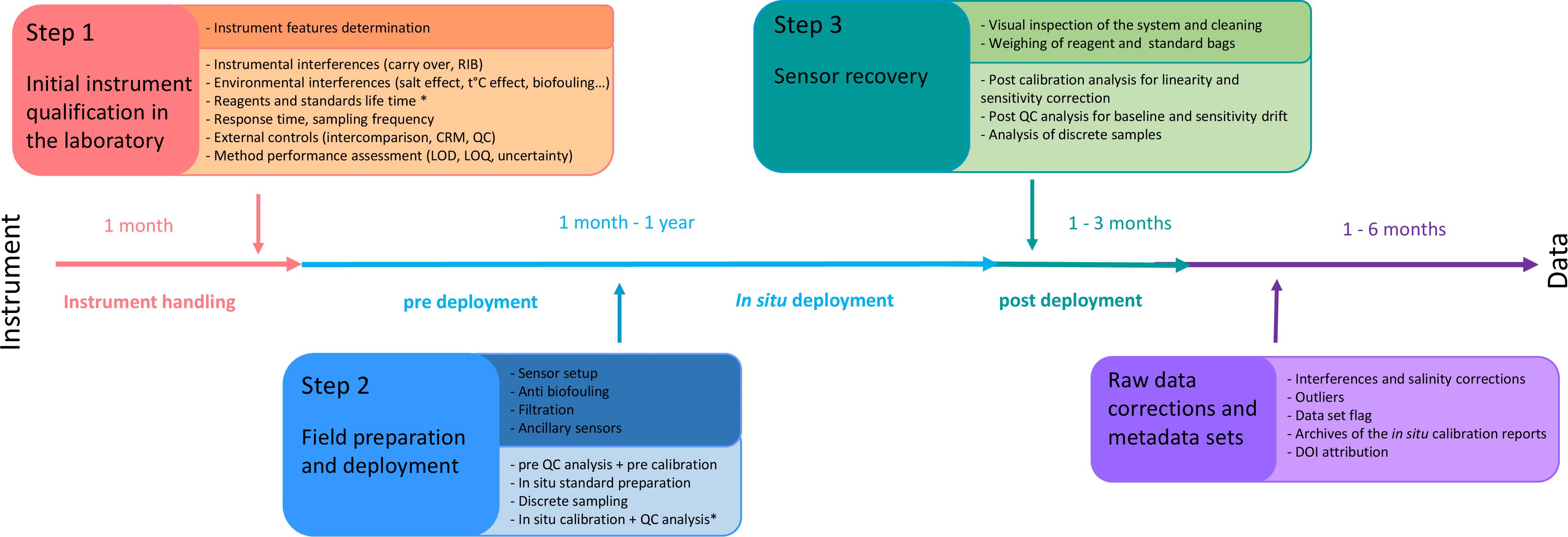
Figure 2. Schematic workflow describing the various steps for using in situ nutrient sensors in seawater (∗ only for wet chemical analyzers).
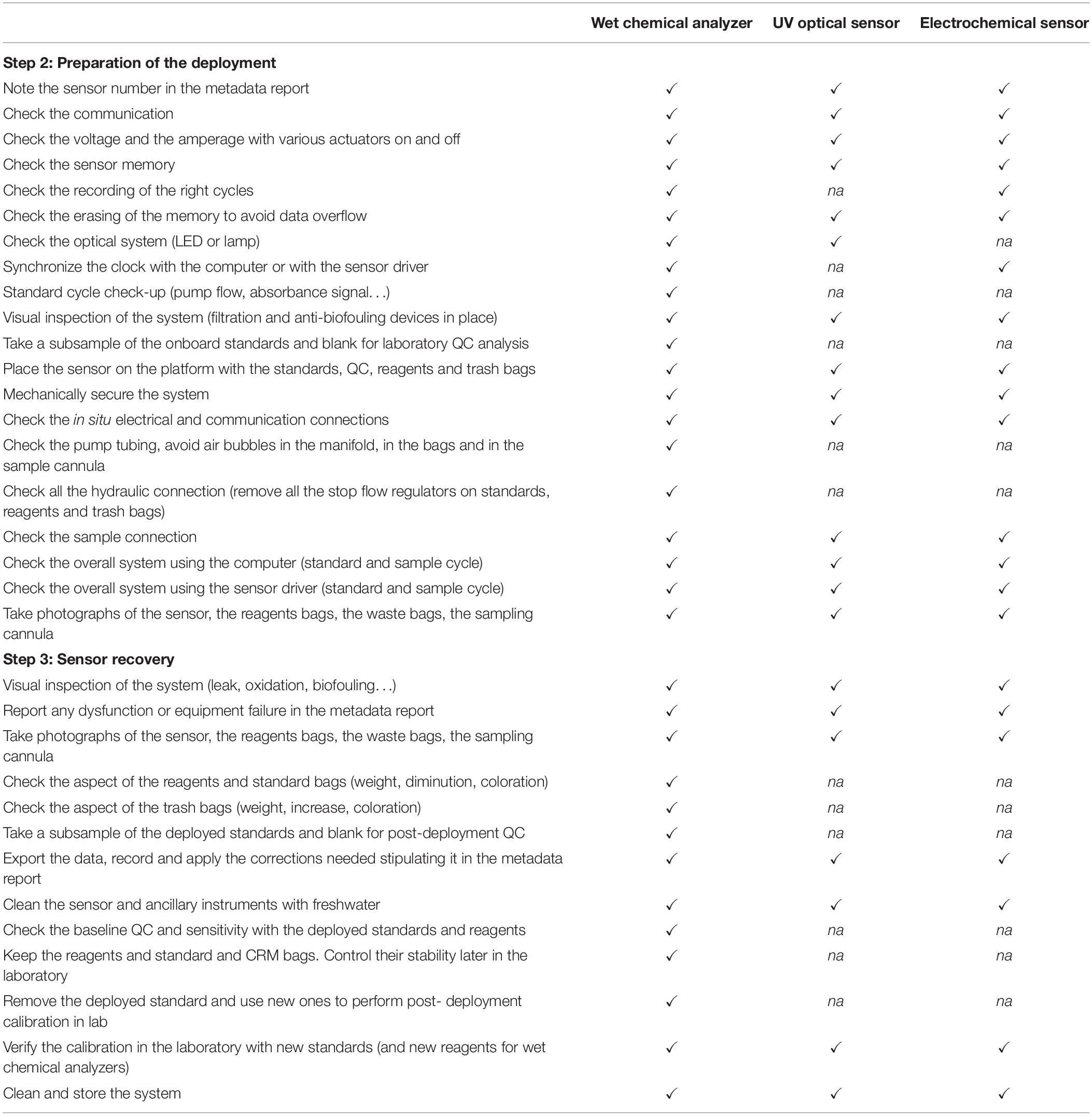
Table 3. Example of a technical check-list to conduct during the deployment of in situ nutrient sensors (to evaluate ✓, not applicable na).
Step 1: Initial Instrument Qualification in the Laboratory
The first assessment is the initial nutrient sensor qualification which is carried out under controlled conditions in the laboratory. It is considered as the reference test for understanding the intrinsic operation of the system. Users should familiarize themselves with the device and determine its capability to make reliable measurements. The technical limitations of the sensors (power consumption, data memory, measurement rate, volume of reagents and standards) have to be carefully evaluated in relation to the applications for which the sensor is intended (study area, deployment modes). The possible impact of instrumental (e.g., corrosion of the infrastructure) and environmental interferences (e.g., salinity and temperature ranges, biofouling) will be simulated in the laboratory. The reagent and standard lifetime will also be verified. Finally, the method performance (e.g., calibration range, limit of detection, linearity, accuracy, and measurement uncertainty) will be assessed. It is recommended to describe in the operational manual the following tests procedures, and to document the results.
Step 2: Field Preparation and Deployment
The field preparation consists of the checking of some essential instrument performances in the laboratory and on-site just before the deployment in a systematic and consistent way. A pre-calibration and pre-Quality Control (QC) samples analysis are required in the laboratory just before the deployment. An overall system check (clock synchronization, memory check, battery) must be conducted on-site (Table 4). When possible, in situ QC analysis and calibration should be planned. It is recommended that, as minimum, additional parameters such as temperature, salinity and pressure are determined at the same time as nutrients because they are important for the interpretation of the results. For long-term monitoring, pictures of the sensor should be taken before and after deployment to archive the effects of biofouling and corrosion.
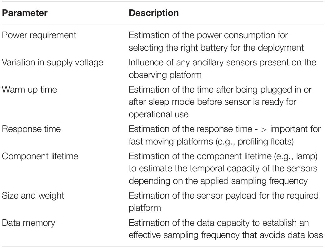
Table 4. Examples of parameters to control before a sensor deployment.
Real-time data transmission is highly desirable as any equipment failure can be detected early, and intervention can be quickly organized to fix faults. Some essential servicing and maintenance for long term deployment should be carried out where and when possible: visual inspection by knowledgeable personnel, maintenance of sensor surfaces by gentle cleaning, changes of pre-filter and filter, running of diagnostics to monitor basic functionalities (power, telemetry, communications, data transmission), and the inspection of the state of hydraulic circuit performance, if present.
Step 3: Sensor Recovery
Finally, the last step lies in the sensor recovery. A visual inspection and taking pictures of the overall system are necessary on site for later diagnosis in the laboratory. The sensors are brought back on board the vessel or taken on land to investigate the overall functioning after deployment (filter, pump flow, battery voltage, flow cell compartment). Actions would have to be taken in response to any equipment failure or faults. Reporting of faults should also be recorded later in the metadata report. For wet chemical analyzers, it is necessary to check the state of reagent bags and their connecting tubes, to look for leaks, blockages or damage, or any reagent precipitation in the bags or deposit build-up on tubing walls. Reagents and standard bags must be measured (by weighing or using a measuring cylinder) to check whether the expected volume has been correctly dispensed in relation to the deployment time so as to interpret eventual discrepancies in the data (leaks, too high or too low volume dispensed, not completed sampling cycles).
The equipment should be cleaned with freshwater, soaked to remove any salt deposits, and dried with pressurized air if necessary. For wet chemical analyzers, the manifold system should be cleaned according to the manufacturer instructions (e.g., cycle consisting of deionized water, HCl 0.1 mol/l and again deionized water), followed by air pumped through the overall manifold. The in situ sensors should generally be stored in the laboratory at ambient temperature, but not in humid conditions or under sunlight.
Essential Good Laboratory Practices for In Situ Sensors
The aim of this section is to consider the best practices implemented and proven for reference instrumentation in the laboratory for application to in situ instrumentation and measurements. These best practices used in SFA are issued from documents such as the GO-SHIP nutrient manual (Hydes et al., 2010; Becker et al., 2019) and Aminot et al. (2009) which describe calibration protocol, instrumental and environmental interferences, external controls and method performance assessment. These recommended practices should only be implemented depending on the sensors being used (Table 5).
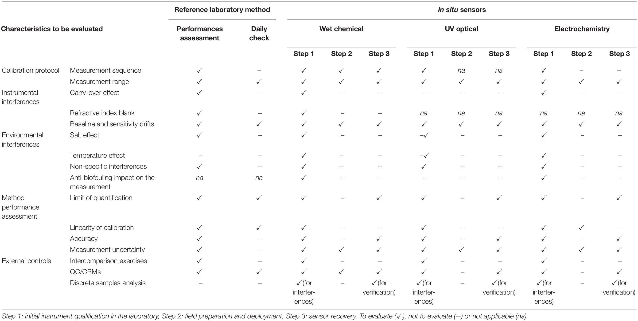
Table 5. A road map for assessing nutrient performances with the laboratory reference method and with each in situ nutrient sensor type.
Calibration Protocol
Units for Expression of Results
The conventional measurement unit adopted for nutrients by marine chemists is μmol/l. The unit μmol/kg is also used for open ocean measurements in order to circumvent ambient pressure and temperature of seawater samples. The conversion is made using the salinity of the sample and the temperature of the laboratory where the analysis is carried out. The mg/l unit is no longer used in the oceanographic community although it is still commonly used by the freshwater community. This concentration in mass by volume leads to an obvious risk of calculation error since it is expressed either in mg/l of the element (e.g., x μmol/l = x ∗ 0.014 mg/l N-NO3–) or in mg/l of the ion (e.g., x μmol/l = x ∗ 0.062 mg/l NO3–).
Reagent Stability
Although some manufacturers provide a guideline to prepare reagents, each laboratory must conduct its own studies to determine the stability of each reagent being used in an analytical protocol regarding the expiration deadline (day to year) and the best storage conditions: type of container (plastic or glass, clear or brown), temperature (fridge or ambient) and light conditions (ambient or dark).
Preparation of Primary Standards
It is essential that materials used to prepare the standards are chemically compatible and clean handling procedures must be adhered to. Primary standards are prepared using analytical-grade salts and UPW. Any new preparation of stock solution must be compared with the old stock solution and an external standard (e.g., MERCK Certipur® NIST certified solution) and validated with a CRM solution. A reference/working range is then made from the newly made stock solution. The two stock solutions and the external standard are diluted to obtain the same concentration (mid measurement range). These three samples are duplicated and analyzed afterward. The results are expressed as a percentage of the sample concentration of the new stock solution. The new stock solution is considered acceptable if the deviations from the old stock solution are not greater than a predetermined value (e.g., 2%). In general, the old stock solution will have the highest concentration due to possible evaporation. This procedure is also recommended to determine the stability of the stock solution for a predetermined period (e.g., one year) with a monthly testing frequency. If the deviation is higher than the expected value, the test should first be repeated and, if found to be consistent, then a new stock solution should be prepared. When the deviation is too high, the expiration deadline or the storage conditions of the stock solution should be reviewed.
The stability of the nitrite stock solution is generally shortest because of oxidation of nitrite to nitrate. Particular attention should be given to the dissolution of sodium hexafluorosilicate for the preparation of the silicate stock solution as this is known to be particularly slow (Aminot et al., 2009). This stock solution must be prepared approximately 1 week before use.
Preparation of Working Standards
Working standards can be prepared with three different categories of diluents: UPW, LNSW, and ASW. Dilution of primary standard with ASW or LNSW presents the advantage to have roughly the same salinity as the samples and will also avoid any differences in color development (see salt effect section). The ideal scenario is to use LNSW that can be obtained by collection of surface oceanic seawater or by filtered and aged coastal seawater (Aminot et al., 2009). Analytical-grade salts used to prepare ASW may contain impurities that can cause much higher nutrient concentrations than those of LNSW: this contamination needs to be checked [especially for Si(OH)4 and NH4+]. The final working standard must always be made up in a solution of comparable salinity to the samples.
Stock solutions should be at room temperature before use to avoid error made on the pipetted volume (Hydes et al., 2010). In order to minimize systematic errors, it is recommended to use at least three different pipettes to dilute the stock solutions and to check the calibration of each pipette on a regular basis. In the laboratory, gravimetry can be preferred to dilution because of the opportunity to conduct weighing operations swiftly and achieve values close to the theoretical mass without leaving time for powder hydration. This approximate weight is then used to calculate the water weight required for dilution.
Measurement Range
The measurement range of a method is defined as the range between the lower and upper concentration of a compound for which it has been established that the method has appropriate levels of accuracy, precision and linearity. There is no advantage of calibrating over a wider measurement range than required, as the uncertainty of the calibration increases with the range. It is therefore preferable to determine several measurement ranges based on expected concentrations in the study areas (e.g., oceanic range, coastal range, estuary range).
It is recommended to prepare at least five working standards evenly distributed over the measurement range. The measurement range should include the LOQ to up to 120% of the highest sample concentration likely to be encountered. Usually the calibrations are conducted from low to high concentrations to avoid carryover problems and the different concentrations should be prepared independently, not from aliquots of the same solution.
Measurement Sequence
The measurement sequence consists first of choosing the sampling rate (number of samples/hour), the sample/wash ratio and the measurement range which must be in accordance with the concentration of the environmental samples to be measured. The measurement sequence includes consecutive analysis of the baseline, blank, standards, baseline blank, QC sample, baseline, n samples (about 10), baseline, n samples, etc… Baseline blank and QC samples are analyzed at regular intervals during the measurement cycle with a consistent position throughout the measurement sequence.
The baseline blank corresponds to the matrix used to prepare the working standards (LNSW, ASW, UPW). The baseline blank is a freshly prepared wash solution that is used to control the baseline drift during a run. A QC sample is a solution of a known concentration close to the highest calibration working standard (best signal to noise ratio). The QC solution is different from the working standards and prepared from an external solution controlled by another laboratory. It is generally a CRM, ready-to-use or to dilute (e.g., MERCK Certipur®).
Consideration of the Calibration Protocol for in situ Sensors
For UV optical and electrochemical sensors, instrument calibration can only be performed in the laboratory or on site prior to/after in situ deployments, not during deployment. If a flow cell is not fitted to the UV sensors, it is required to fully immerse them for calibration which can be a tricky process. For commercially available wet chemical analyzers, the current best practice recommendation is to carry out pre-deployment calibration in the laboratory and not to send it to the manufacturer. This is due to the requirement of using the same in house reagents and working standards for deployment and pre- and post-deployment checks to ensure measurement stability. The solutions can be split into three batches, one for each pre-deployment, deployment and post-deployment tests, and placed into the same plastic chemical storage bags that will be used during the deployment. All the reagent and standard solutions must be degassed to avoid formation of air bubbles whilst in deployment, and should be cooled and kept in the dark during shipment to the deployment platform. A secure and suitably sized waste bag should be installed to prevent environmental contamination.
Because the in situ nutrient wet chemical analyzers may be subject to a range of temperatures and pressures during deployment, a full assessment of reagents and standards lifetime must be conducted at the temperatures and pressures expected during the deployment. If necessary, the longevity of standards can be increased through addition of preservative (e.g., chloroform 0.01%; Beaton et al., 2017). To resolve freezing effects in polar areas, antifreeze may be added in the reagents (e.g., up to 30% of spectrophotometric grade ethylene glycol; Beaton, 2012). Certain standards and reagents are light sensitive and/or easily oxidized. The use of appropriate containers, such as plastic bags impermeable to light and gases (e.g., coated with aluminum; RestekTM; ChemwareTM) can be used to extend deployment periods. If stabilization of standards and reagents cannot be achieved, the deployment period should be modified accordingly.
The in situ sensor calibration is similar to the procedure performed for the laboratory reference method: a succession of standards with concentrations chosen for the specific deployment, blanks, CRM and/or in-house standard QC. Generally, at least three working standards are used for in situ sensor calibration with concentrations evenly distributed over the measurement range expected on-site. The concentration of these standards must be determined by a measurement using a reference laboratory instrument. This calibration should be carried out at the same temperature and salinity as close as possible to expected deployment conditions.
Instrumental Interferences
Baseline and Sensitivity Drifts
In theory, the analytical response of an instrument should not fluctuate during a measurement cycle. In practice, this response can vary and this change in magnitude of the output signal is called a drift. Drift control has to be part of a quality system and should be formally reviewed on a regular basis. By repeating “baseline blanks” during a run, changes in the baseline can be compensated for. It works on the basis that drift is constant and linear between baseline determinations. This drift is easily corrected by the software. Baseline drift is often due to coating of the flow cell or to background contamination.
The approach to correct the sensitivity drift is similar to the baseline drift. A sensitivity drift is observed when the height of the QC, regularly placed in the run, changes gradually. The correction is also a linear interpolation. This sensitivity drift should be treated with caution to be sure that it is really due the analytical system (electronic, hydraulic, coating effect) and not to a change of the QC nature (contamination, evaporation). When QC concentrations are recorded on a control chart, it is possible to prove that the measurement procedure works within given limits. If a value is outside the control limits, corrective actions must be taken to identify and eliminate the sources of errors. The control chart can also be used for the determination of the measurement uncertainty.
Carry-Over Effect
Carry-over is a phenomenon that occurs when the dispersion of the sample in the flow is high. The dispersion plume is responsible for transferring a fraction of the compound to be analyzed from one sample to the next. The importance of the carry-over effect is related to the concentration of the previous sample: it is reduced or eliminated by analyzing samples from low to higher concentrations. The first way to correct this effect consists in increasing the time period between two successive samples. Because it is not always possible to reduce the sampling rate, the second method is based on the analysis of one high standard either analyzed twice again or followed up with a duplicated analysis of a lower concentration standard. The calculations for correction are based on the difference of the signal heights (Aminot et al., 2009). The carry-over should be determined at several points in a run as it can be sensitive to any system changes.
Refractive Index Blank
The RIB is specific to the flow analysis method being used and is considered equivalent to the sample blank. It is the signal that a zero concentration will have produced for a given salinity. In practice, at the end of the run, the key color-forming compound is removed from reagent solution and the RIB is determined by reanalyzing a few selected samples. The RIB signal rarely exceeds 0.1 μmol/l for all nutrients except some coastal waters which can be naturally colored by organic matter (Aminot et al., 2009). However, it is important that the RIB is determined and where required the final concentrations must be adjusted accordingly.
Consideration of the Instrumental Interferences for in situ Sensors
Baseline and sensitivity drift will be estimated during the analytical performance assessment using blanks and QC standards as it is performed for the reference laboratory method, and this applies to the three main in situ techniques. When possible, these drifts should also be carefully checked during the deployment, ideally at the start of each sample run, because it is strongly related to changes in the instrument behavior (electronic, hydraulic and heat dissipation by electronic components).
Carry-over corrections are not required for UV optical sensors. Carry-over correction for flow-through analyzers is not achievable in situ, the sample being unique. It is therefore essential to avoid this effect by setting a suitable sampling rate and flushing time between samples that allows the system to return to its initial baseline before the measurement of the next sample. If the user can not adjust this in the sensor settings, a global carry-over correction coefficient might be calculated in the laboratory (Aminot et al., 2009) and applied for correction after deployment.
RIB corrections are not required for UV optical and electrochemical sensors. It is also not possible to determine in situ the RIB occurring with wet chemical analyzers because this procedure consists of reanalysis of a sample without addition of the key color forming reagent. This is therefore an effect that needs to be carefully evaluated during primary tests in the laboratory to serve as a reference for the in situ measurements.
Environmental Interferences
Salt Effect
Salt effect is defined as the signal variation obtained for the same concentration as a function of salinity. The salt effect can reach 10–20% on a salinity range and it is not always linear. The salt effect is specific to each analytical method and should be estimated for each instrument especially when measurements are done in coastal waters and estuaries or when UPW is used for baseline and/or working standards. A procedure for correction of the salt effect is presented by Coverly et al. (2012).
Temperature Effect
The effect of temperature on the measurement is unusual when using a laboratory analyzer because generally most laboratories are equipped with air conditioning and temperature mediated reactions are controlled by heating baths. However, it is important to ensure samples are brought to the laboratory temperature prior to analysis (e.g., sampling in polar or tropical waters).
Non-specific Interferences
Interferences are negligible in natural unpolluted waters. However, when studying particular areas (estuaries, mangrove swamps, hydrothermal events), the potential impact of other chemical elements (e.g., high suspended matter, dissolved organic matter, humic acids, sulfide) present at a concentration greater than that usually encountered in seawater must be tested. They are estimated by spiking seawater of known nutrient concentrations with the possible interfering compound. The concentration at which a significant effect (positive or negative) is observed should be carefully related to typically observed concentrations at the study site. Particulates can be easily eliminated by filtration (e.g., Acrodisc® syringe filters 0.45 μm) or centrifuging the sample. It is also essential to remove particulate phosphate that may contribute to the sample reading from the dissolved fraction of phosphate.
Consideration of the Environmental Interferences for in situ Sensors
If the sensor is deployed in an environment which experiences a large range in salinity then testing must be carried out to determine the magnitude of the effects upon the in situ sensors, so that the results can be corrected post-deployment. It is also recommended to measure salinity simultaneously with nutrient concentrations. To minimize the salt effect, standards must be prepared in LNSW or ASW, these suitably diluted with UPW, to match the expected salinity during deployment.
Deployment of in situ sensors in non-temperate areas, such as surface mooring in polar latitudes or tropical regions, or as FerryBox systems located in a ship engine room, requires specific sensor preparation and operational use. The impact of temperature should first be evaluated in the laboratory as a function of the expected environmental conditions. Some wet chemical analyzers use a thermostat to regulate the optimal reaction conditions (e.g., CHEMINI for ammonium detection at 40°C).
Because particle concentrations can exert an impact on measurement performance, pre-filtration may be necessary. For small manifolds, such as LoC systems, filtration is highly recommended to avoid blocking the channels of the microfluidic system (Grand et al., 2019). The correct choice of filter pore size depends on the particle dynamics in the deployment location, acknowledging that this may or may not be known at the time of deployment. Filter pore sizes should not be too small because there is a risk of filter clogging and impeding sample delivery to the device. The use of a pre-filter prior to a smaller pore size filter can be essential (e.g., Millex syringe Merck Millipore). Minimizing flow over the filter by minimizing the sample volume helps filters last longer. The material of the filter and pre-filter should be carefully selected to avoid any contamination of the system (Teflon, glass fiber). A more sophisticated system can sometimes be used, e.g., a hollow- fiber cross-flow filter module for FerryBox applications. Discrete seawater samples can be collected as often as possible at the deployment site for later laboratory measurements to determine the evolution of the potential environmental interferences.
The growth of organic films and organisms on instrumentation surfaces immersed in water (termed biofouling) may affect the analytical and data quality, particularly in highly productive coastal regimes, but also in the open ocean after extended deployment periods (Griffiths et al., 2001; Adornato et al., 2009). The impact of biofouling is less important for instruments using flow conditions (wet chemical analyzers) than static conditions (UV and electrochemical sensors without a flow cell). Faimali et al. (2014) proposed a comprehensive overview of biofouling prevention practices and recommendations. Anti-fouling measures to prevent or reduce this effect come in two forms: passive chemical guards (removable or fixed copper components) and mechanical devices used intermittently during measurement cycles (wipers with nylon bristles or silicon blades). The generation of hypochlorite by seawater electrolysis can also be a solution to avoid major biofouling growth (Sarrazin et al., 2007).
External Controls
After validation of the analytical method, an external quality control can be implemented by participating in intercomparison exercises and using CRMs. These are part of operational procedures which are essential for ensuring long term control of accuracy and good comparability of data among laboratories. Quality control charts should be plotted for each CRM to ensure that the results are consistent with the analytical specifications.
Intercomparison Exercises
An intercomparison exercise consists of the analysis of homogeneous and stable materials by different laboratories, with the analytical method of their choice or with a recognized method, and the comparison of the results. Intercomparison exercises for measurement of nutrients in marine water are organized by a number of institutions, the main international one being QUASIMEME5. Following ICES exercises in the 1990s (Aminot and Kirkwood, 1995), a number of intercomparison studies have also been conducted recently by the Meteorological Research Institute (MRI) in Japan (Aoyama et al., 2007, 2010, 2016, 2018) with the motivation to develop CRMs for nutrients in seawater to improve the comparability of global oceanic nutrient data.
Certified Reference Materials
Certified reference materials are characterized by a metrological validation procedure, accompanied by a certificate that provides the value of the specified property and its associated uncertainty (ISO/Guide 30, 2015). CRMs should have the same characteristics (concentration range and salinity) as the samples that are currently analyzed by the laboratory so that analytical errors can be identified. CRMs should be applied to ensure consistency between analysts and in day-to-day operations, so as to guarantee comparability and traceability of data.
Nutrients CRMs for seawater have only become readily available in recent years6. They have been developed since the 2000s by: the National Research Council Canada (NERC, MOOS CRM; Clancy and Willie, 2004), VKI Eurofins Denmark, the Korean Institute of Ocean Science and Technology (KIOST) and the General Environmental Technos Co., Ltd. (Kanso) in Japan (Ota et al., 2010). These CRMs are essential to achieve one of the most important goals of the chemical oceanographers, i.e., allowing the comparability of nutrient analyses with a level of analytical precision better than 1% (Hydes et al., 2010; Rees et al., 2018). CRMs also facilitate the control of accuracy, and whether it can be maintained, by implementing time control charts (ISO/TS 13530, 2009).
Consideration of the External Controls for in situ Sensors
Typically, intercomparison exercises involve sending aliquots of a sample to multiple institutions. However, the sample volumes commonly delivered for intercomparison exercises are small (about 100 ml) and therefore exclude the participation of many in situ nutrient sensors, particularly the UV optical units without an integrated flow cell, that need to be submerged. CRMs present the same disadvantage due to the sample volume currently proposed by the manufacturers.
Discrete samples can be collected next to the deployed nutrient sensor and analyzed with reference laboratory methods. To better calibrate the data gathered during the deployment, this sampling should be done at least during the installation and prior to the recovery, every additional sampling collection during the deployment being beneficial. For moored/buoy systems, CTD profiling, AUVs and FerryBox deployments, a discrete water sampler unit can also be set up alongside to the nutrient sensor deployment to collect samples for later laboratory analysis, especially in the case of UV optical and electrochemical sensors for which the sensitivity drift cannot be controlled in situ. This comparison of sensor and conventional nutrient measurement is the primary tool for control of trueness and accuracy of sensor-based field measurements.
Method Performance Assessment
Sensor calibration, measurement range, accuracy, sensitivity, resolution, measurement uncertainty, limit of quantification/detection are the main specification requirements for most analytical methodologies. To facilitate comparison between analytical results, the definitions of the terms describing the performance of any analytical method should be the same for all users. It is widely accepted to follow the definitions of the VIM (JCGM, 2012).
Method validation is the process of assessing whether an analytical method is acceptable for its intended purpose. The validation study demonstrating the suitability of a novel method should be carried out before routine adoption. All conditions that are considered critical should be controlled and evaluated. Basic requirements include the determination of (1) the limits of detection and quantification, (2) linearity, (3) accuracy, and (4) measurement uncertainty.
Limit of Detection and Limit of Quantification
The LOD is a value which can affirm that a sample is different from a blank sample, while the LOQ is the concentration that can be reasonably determined with an acceptable level of accuracy and precision (ISO/TS 13530, 2009). Separate determinations of LOD and LOQ may be required for different measurement ranges and for different matrices.
The LOD of a method should not be confused with the lowest instrumental response which is determined using the signal to noise ratio. The ISO/TS 13530 (2009) proposed three methods to determine LOD based on: (1) the standard deviation of blank samples (or very low concentration samples), (2) standard deviation of the method (from calibration), (3) baseline noise. The most commonly used one is the first one, which is based on the work of Taylor (1990). It consists of measuring a large number of blanks (n ≥ 10) and to express the LOD as a mean sample blank value plus three standard deviations (+3 s). Various conventions have been applied to estimating the LOQ. The most common recommendation is to quote the LOQ as the blank value plus 10 times the repeatability standard deviation or sometimes as three times the LOD. The essential step after the estimation of the LOD and LOQ is the verification: analysts need to show that they are able to detect/quantify the analyte at the estimated limits in each matrix. This step is needed to be able to compare LOD and LOQ of different laboratories with the same quality targets.
Linearity of Calibration
The linearity of the calibration of an analytical method is its ability to generate a signal that is directly proportional to the concentration. If the use of the correlation coefficient should be avoided, testing for lack of fit by examining the residuals after linear regression is statistically valid and easy to perform (ISO, 8466-1, 1990; Hydes et al., 2010). There is no need to set the intercept to zero unless there is evidence that it is not statistically different from zero (e.g., “slope only” in SFA).
Accuracy
The accuracy of a measurement result (ISO/TS 13530, 2009) describes how close the result is to its true value and therefore includes the effect of both trueness and precision. It is considered as describing the total error.
Trueness is the estimate of the systematic error. Measurement trueness describes the closeness of agreement between the average of an infinite number of replicate measured values and a reference value (e.g., CRM). To take into account any variation between runs, trueness must be determined over several days. Bias is the quantitative expression of trueness.
Precision is a measure of the spread of repeated measurement results obtained under stipulated conditions (repeatability and reproducibility). Repeatability is the analysis of a sample several times over a short period (e.g., the same day), by one person in one laboratory, and with the same instrument. Reproducibility is the analysis of a sample under varying conditions (e.g., different times and days, by several persons). Precision depends only on the distribution of random errors; it gives no indication of how close those results are to the true value. Standard deviation, obtained from multiple measurements with the same sample, is the quantitative expression of precision.
Measurement Uncertainty
The VIM definition of uncertainty (JCGM, 2012) is a “non-negative parameter characterizing the dispersion of the quantity values being attributed to a measurand (quantity intended to be measured), based on the information used.” Uncertainty estimation of chemical analysis results is associated with the result of a measurement and is now a standard requirement (Eurachem CITAC guide, 2012). Results without an uncertainty estimate cannot be considered as complete.
EUROLAB (2007) gives an overview of the main approaches currently used for uncertainty evaluation (Figure 3): (i) the modeling approach (see the GUM; JCGM, 2008), (ii) the single-laboratory validation approach, (iii) the validation approach based on interlaboratory studies (ISO 21748, 2017), and (iv) the approach using intercomparison exercises data. Uncertainty information requires attention to the scope and form of the data concerned. For example, the results obtained using “empirical” approaches normally refer to the typical performance of a specified test procedure on specified test objects, while uncertainty estimates obtained using the modeling approach most often refer to individual measurement results. Therefore, most practical uncertainty estimates involve elements of both modeling and “empirical” approaches. Several guidelines are available for the estimation of uncertainty in quantitative testing (EA Guideline Ea-4/16, 2003; EUROLAB, 2006) and in the field of water analysis (ISO 11352, 2012). The Finnish Environment Institute (SYKE) makes available free software (Mukit Copyright (c), 2012) which can be applied to estimate measurement uncertainty according to ISO 11352 (2012).
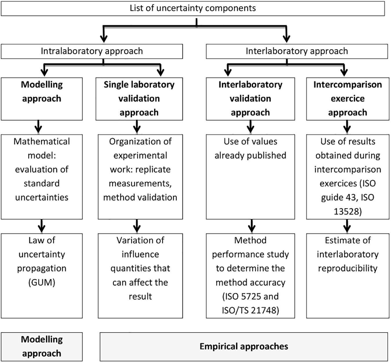
Figure 3. Uncertainty estimation approaches (from EUROLAB, 2007).
Consideration of Methods Performance Assessment for in situ Sensors
Determination of the limit of quantification, accuracy and measurement uncertainty should be carried out as proposed for the laboratory standard method for all in situ nutrient sensors. In this way, the quality control of field measurements will become as stringent as those for laboratory analysis and this for all the analytical approaches. One approach to determine uncertainty of nutrient measurements from LoC sensors is also presented by Birchill et al. (2019). Quality control charts for the analysis of QC samples used by wet chemical analyzers should be recorded and checked to make sure that the analytical performance is continuously maintained and in accordance with the requirements.
Raw Data Treatment for In Situ Sensors
In some studies, raw sensor signals are transmitted via telemetry to shore based data stations, and near real time data can then be made available. If not, data will be stored on the sensor or platform, extracted later and archived to avoid any data loss. Different corrections (Figure 4) are necessary to convert raw data to final data. We describe here the corrections that apply to wet chemical analyzers because they are the most common system. All these corrections are not required for UV and electrochemical sensors because they do not use chemical reagents, cannot yet be calibrated in situ and do not require verification of in situ baseline and sensitivity drifts. The corrections of these two technologies are then only based on pre and post deployment calibration measurements and on measurement of discrete samples taken in the same geographic area as the sensors.
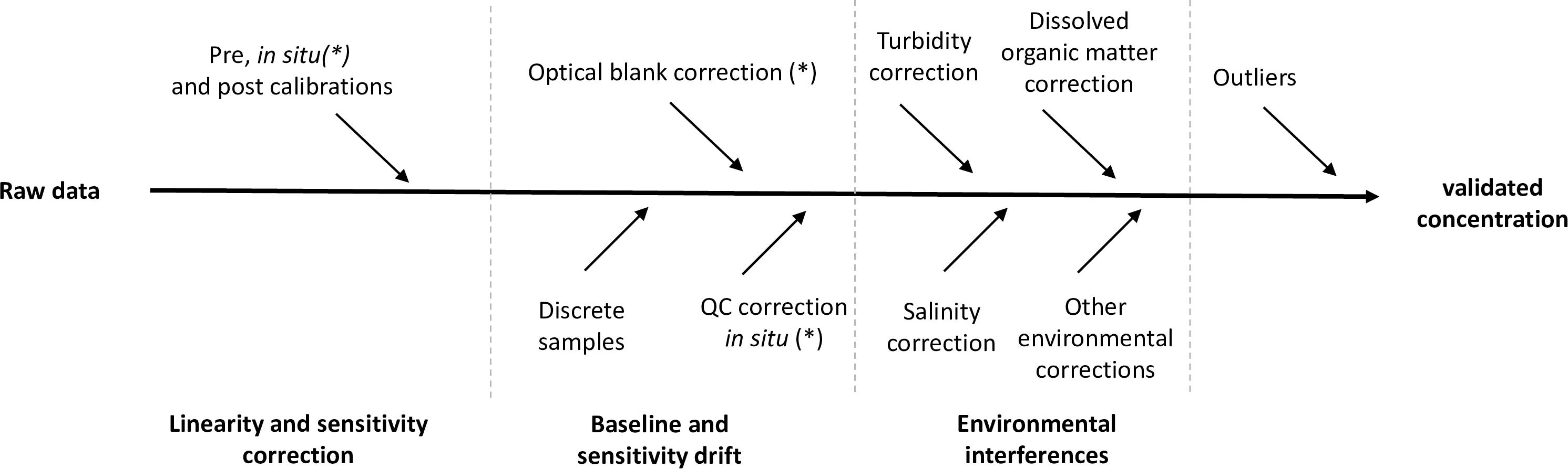
Figure 4. Schematic view of the transformation of raw data across the various correction steps toward final nutrient concentration; some corrections might be applicable only in the case of wet chemical analyzers (∗).
Note that for some manufactured systems, software calculations can sometimes be configured by default (automated RIB calculation) and that some automatically applied corrections are not always explained in the instrument manuals (e.g., RIB correction with WIZ, salinity and temperature correction for SUNA).
Linearity Corrections for in situ Sensors
The chemical quality of the in situ reagents and standards may vary during the deployment period and this may affect the sensitivity and/or linearity of the method. The recovered sensor should be then carefully calibrated after deployment using the field standards and reagents, and then also with fresh reagents and standards.
The linearities of pre, on-going and post-deployment calibrations (Table 6) are then cross-compared according to the residual calculation method. No linearity correction should be made if all linearities are acceptable. If there is a difference between linearities after deployment between in situ and fresh reagents, no correction should be made because it is already taken into account by the in situ calibration itself. On the other hand, if a difference of linearity is apparent between in situ and fresh standards, a correction of linearity should be applied because of the variation in standard concentration. The linearity obtained with the fresh standard and the in situ reagents will be used to calculate the sample concentration. If the in situ reagents/standards calibration linearity and fresh reagents/standards calibration linearity are conflicting, the deployment results are unusable and flagged as “false.”
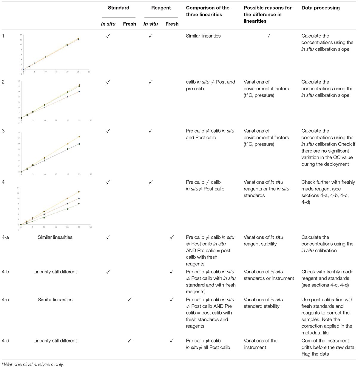
Table 6. Comparison of the linearities obtained with the pre- (yellow dots), in situ (blue dots) and post- (green dots) calibrations made with in situ∗ or freshly made reagents and standards.
The correction of the linearity for UV and electrochemical sensors is based on the same principle but only with pre and post calibration.
Sensitivity and Baseline Corrections for in situ Sensors
Sensitivity and baseline drifts are regularly checked by measuring blanks and QC for wet chemical analyzers. Discrete samples can also be used to correct systemic errors for UV optical and electrochemical sensors. The sensitivity drift is not evaluated by using the slope of the calibration line but by plotting all the QC concentrations in a control chart which allows checking that the sensor works within given limits. The baseline drift is typically due to cell coating, and if observed, it is corrected by a simple linear interpolation between two successive blanks. There are three possible scenarios (Table 7):
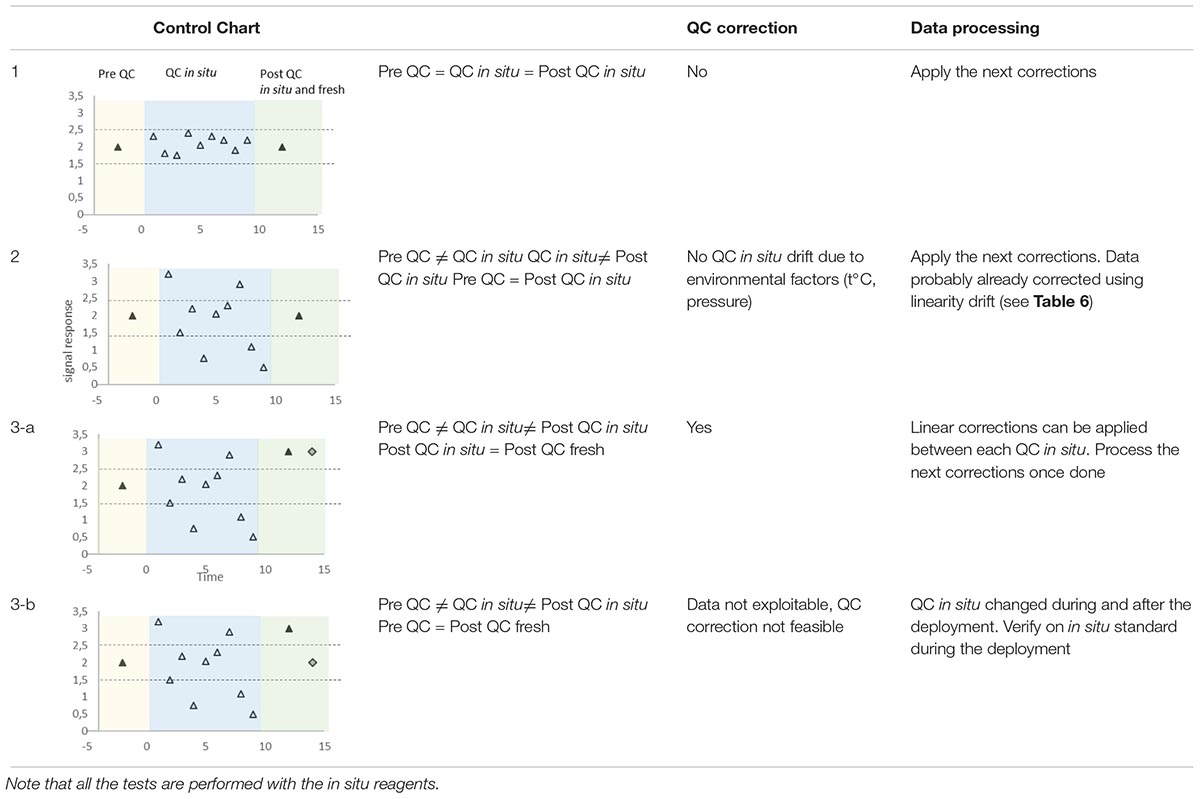
Table 7. Various scenarios and associated corrections (yellow and green areas correspond to tests performed in the laboratory before and after deployment, blue areas are linked to in situ deployment, black triangles stand for analysis of QC before deployment and after deployment (same QC as in situ) in the laboratory, white triangles for in situ QC during deployment, and gray diamonds for freshly prepared QC analyzed after sensor recovery).
(1) all the QC concentrations are included within the recommended limits: no sensitivity correction is to be undertaken,
(2) some in situ QC concentrations are outside of the recommended limits of the control chart but the post-deployment QC measurements carried out with in situ QC solutions are adequate: the changes are likely due to temperature and/or pressure variations, no correction to apply
(3) some in situ QC concentrations are outside of the recommended limits of the control chart just as the post-deployment QC measurements carried out with in situ QC solutions: a second post-deployment control must be conducted with fresh QC solutions. (3-a) If the concentration of this additional control is similar to the ones obtained with the in situ QC solution, a linear interpolation correction is made between each successive QC. (3-b) In contrast, if there is a difference between these two concentrations, it means that the concentration of the in situ QC solution has changed during the deployment. This scenario is similar to that showing a change in the concentration of the standards during deployment. Because the correction of linearity should have been applied before examining the QC, results mean that only the QC concentration has changed. The sensitivity correction is then impossible to achieve.
Correction of Environmental Interferences
When the study area is subject to pronounced salinity variations, the correction factor of the salt effect, which was calculated before deployment, should be applied to the raw data. The potential impact of naturally occurring interferences in the waters of the study area waters (e.g., turbidity, dissolved organic matter, sulfide) is evaluated after the deployment by measuring their concentrations in the discrete samples. The raw nutrient values are then corrected if needed.
Outlier Data
Outlier values below the LOD and higher than the maximum concentration of standards should be flagged as questionable.
Metadata Sets
More widespread use of in situ sensors is expected to result in a significant increase in the amount of marine nutrient data. An archive of all on-site sensor deployment reports should be maintained for an indefinite period of time. These reports should describe all preparation, field and post-deployment performance checks.
Real Time Data
Whilst physical oceanography has long been dealing with high real time data volumes, most of the nutrient sensors are stand-alone data recording units that are not working via near real-time access. The only near-real time nutrient data are obtained from sensors deployed on Ships of Opportunity, where internet connection can be permanent (e.g., SYSTEA Micromac), and from sensors integrated on gliders which are communicating via a satellite transmission system.
The demand of real-time processing poses a challenge because traditional approaches to quality control are no longer practical (Campbell et al., 2013). Basic automated quality checks procedures permit to verify if the sensor is working well (e.g., detection file format error, missing values, low battery, above or below ranges), quickly process data, identify problems in near real time. However most of the analytical corrections should be carried out post deployment. Real time data have then to be considered as raw data that need to be corrected after deployment with metadata. The US Integrated Ocean Observing System has published guidance on the quality control of real-time dissolved nutrient data (U.S. Integrated Ocean Observing System, 2018).
Delayed Mode Data
The data must be accessible and associated with rich and comprehensive standardized set of metadata which follows the requirements of the GO-SHIP manual (Becker et al., 2019) and the additional information list in Table 8. The metadata report should be accessible with unrestricted access, should be interoperable and understandable so as to enable traceability.
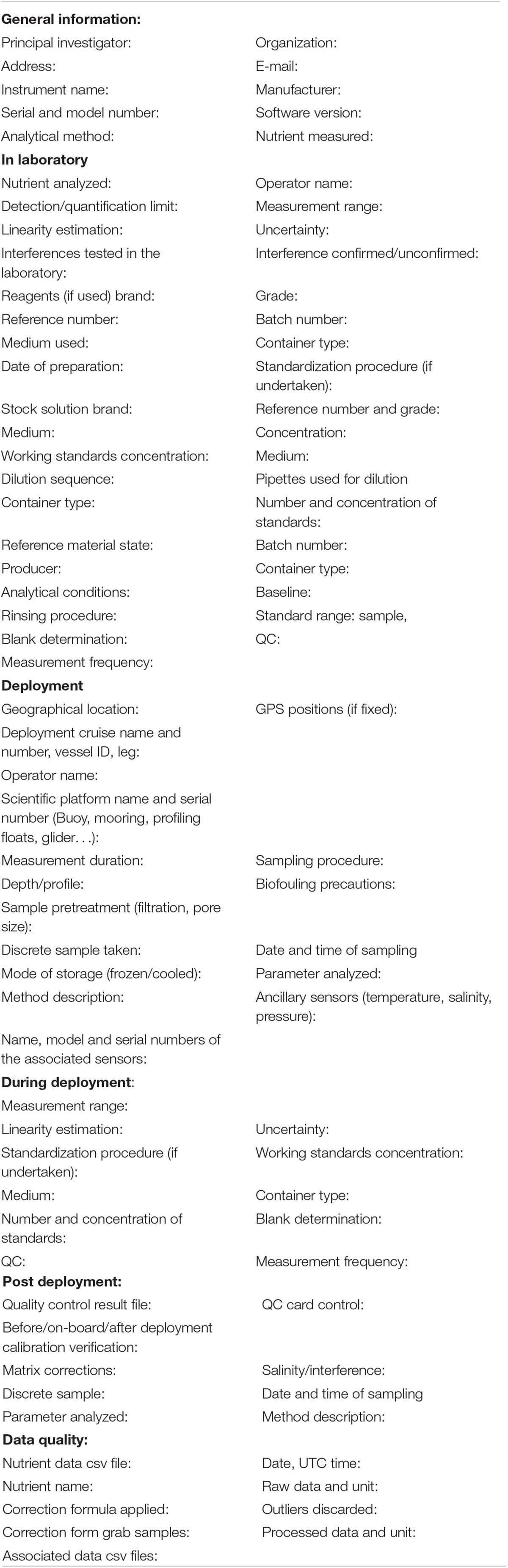
Table 8. Example of form to report metadata of in situ nutrient measurements.
Quality Control of the Data Set
The FAIR (Findable, Accessible, Interoperable, and Re-usable) principles must guide the nutrient data management system (Tanhua et al., 2019). Quality control processes and standards are critical for producing precise and accurate data (Bailey et al., 2019). Documents have been already published to facilitate the exchange and integration of multi-disciplinary oceanographic data (Intergovernmental Oceanographic Commission IOC, 2013) or to establish data quality controls (U.S. Integrated Ocean Observing System, 2017). Successful quality controls require especially convergence in standards in flag schemes. Flagging the data allows enhancing data reliability and conveys information about individual data values, typically using codes. Flags can be highly specific to individual studies or standardized across all data for a program or oceanographic institution.
Given the current state of nutrient sensor technology, only personnel with intimate knowledge of sensor operation are competent to assess the quality status of the data. If data from nutrient sensors are not so far accepted into databases, this is due to a lack of agreed quality control procedures at the point of data being submitted to the database. This can be explained in part because of the small number of laboratories currently using these in situ sensors which has therefore only provided a small amount of experience feedback compared to standard laboratory analysis methods. We hope that this article will help to build consensus on the quality control procedures necessary for in situ nutrient sensor data to be accepted into international databases.
Attribution of DOI
A DOI is a unique alphanumeric string to identify content. An increasing number of publishers require authors to make all the data described in their articles fully available without restriction. If the dataset is available for re-use (e.g., to check a result), it could accelerate scientific progress. Sharing nutrient data is seen as key to improving data integrity and to enhancing transparency and reproducibility in oceanography. Open data is also a societal demand.
Conclusion and Future
The aim of this paper is to help to transfer knowledge on quality procedures implemented for the standard laboratory methods to in situ nutrient sensor operations to get data as close as to the true concentration with the best estimation of analytical performances. The described procedures and corrections applied are intrinsically linked to the technology of the nutrient sensor and of the deployment platform. Not every deployment needs to have the same accuracy and uncertainty but it is required to explain their calculations and to record them in the metadata sets associated. The establishment of a website forum, where metadata forms of all type of sensors could be shared, would be a great advance. This site will be also a useful resource for the oceanographic community to promote and improve the calculations of correction factors for each type of sensor.
The European Union Horizon 2020 projects, AtlantOS and JERICO, are working on the improvement of a clear vision of the observing system of the ocean, and monitoring of nutrients plays an important part in this goal. However, one of the conclusions of these projects is that there is a lack of long-term sustainable funding for this research, which makes it difficult to maintain reliable in situ nutrient observations in the coming years. There is therefore an urgent need to strengthen and coordinate collaborations between research groups, accredited analytical laboratories and industry. In addition, the development of reference materials suitable for in situ sensors, as well as providing deployment platforms to conduct in situ intercomparison exercises with different sensor technologies, has become essential for users.
In the near future, according to the evolution of electronics and the emergence of cost-effective materials, the challenge to develop new instruments capable of performing measurements in all salinity and temperature ranges and under a broad range of nutrient concentrations seems achievable but is currently difficult to meet.
Author’s Note
This article is a compilation of the discussions from the workshop “Interoperability of Technologies and Best Practices: in situ applications to nutrient and phytoplankton fluorescence measurements” organized in Brest (France), December 4–6, 2018.
Data Availability Statement
The raw data supporting the conclusions of this manuscript will be made available by the authors, without undue reservation, to any qualified researcher.
Author Contributions
AD and AL-H co-led the initiative of this work, and coordinated and contributed equally to the writing and the revision of the manuscript. CB, AB, DB, NGu, MK, DM, IS, EW, NGr, and EA reviewed and provided inputs on the manuscript. NGr and EA respectively led the subtask 2.4.1 “Sensors for nutrients” of the JERICO project and the task 6.2 “Common metrology and best practices” of the AtlantOS project.
Funding
This article was funded by AtlantOS and by JERICO.
Conflict of Interest
The authors declare that the research was conducted in the absence of any commercial or financial relationships that could be construed as a potential conflict of interest.
Acknowledgments
Many thanks to all the workshop participants for the very interesting presentations, and the rich and constructive debates. We would like to acknowledge Florian Caradec, Romain Davy, Emilie Rabiller, and Léna Thomas for their technical support especially during the practical courses of the workshop. We are grateful to Chantal Compère for her assistance in the local organization of this workshop. We also thank all the people involved in the development and deployment of the nutrient sensors.
Abbreviations
μ LFR, μ Loop Flow Reactor; ACT, (Alliance for Coastal Technologies); ASW, Artificial Sea Water; AtlantOS, Optimizing and Enhancing the Integrated Atlantic Ocean Observing Systems; AUVs, autonomous underwater vehicles); CRMs, certified reference material); CTD, Conductivity Temperature Depth; DOI, Digital Object Identifier; EOVs, Essential Ocean Variables; FIA, flow injection analysis; GOOS, Global Ocean Observing System; GO-SHIP, Global Ocean Ship-based Hydrographic Investigations Program; GUM, Guide to the expression of Uncertainty in Measurement; ICES, International Council for the Exploration of the Sea; JERICO, Joint European Research Infrastructure Network for Coastal Observatories; LNSW, low nutrient sea water; LoC, Lab-on-Chip; LOD, limit of detection; LOQ, limit of quantification; QC, quality control; QUASIMEME, Quality Assurance of Information for Marine Environmental Monitoring in Europe; RFA, reverse flow analysis; RIB, refractive index blank; SCOR, Scientific Committee on Oceanic Research; SFA, segmented flow analysis; UPW, UltraPure Water; UV, ultraviolet; VIM, International Vocabulary of Metrology; WOCE, World Ocean Circulation Experiment.
Footnotes
- ^ www.goosocean.org/eov
- ^ https://www.atlantos-h2020.eu/
- ^ http://www.jerico-ri.eu
- ^ http://www.act-us.info/database.php
- ^ www.quasimeme.org
- ^ www.jamstec.go.jp/scor
References
Adornato, L., Cardenas-Valencia, A., Kaltenbacher, E. A., Byrne, R. H., Daly, K. L., Larkin, K. E., et al. (2009). “In situ Nutrient Sensors for ocean observing systems,” in Proceedings of OceanObs’09: Sustained Ocean Observations and Information for Society, eds J. Hall, D. E. Harrison, and D. Stammer, (Auckland: ESA Publication), doi: 10.5270/OceanObs09.cwp.01
Aminot, A., and Kérouel, R. (2007). Dosage automatique des nutriments dans les eaux marines. Quae. Rennes: Cloitres Imprimeurs.
Aminot, A., Kérouel, R., and Coverly, S. (2009). “Nutrients in seawater using segmented flow analysis,” in Practical guidelines for the analysis of seawater, ed. O. Wurl, (Boca Raton, FL: CRC Press) 143–178.
Aminot, A., and Kirkwood, D. S. (1995). The fifth ICES intercomparison exercise for nutrients in seawater. ICES Coop. Res. Rep. Ser. 213, 1–78.
Aoyama, M., Abad, M., Anstey, C., Ashraf, M. P., Bakir, A., Becker, S., et al. (2016). IOCCP-JAMSTEC 2015 Inter-laboratory calibration exercise of a certified reference material for nutrients in seawater. IOCCP report number1/2016. Yokosuka: Japan Agency for Marine-Earth Science and Technology.
Aoyama, M., Becker, S., Dai, M., Daimon, H., Gordon, L., Kasai, H., et al. (2007). Recent comparability of oceanographic nutrients data: Results of a 2003 intercomparison exercise using reference materials. Anal. Sci. 23, 1151–1154. doi: 10.2116/analsci.23.1151
Aoyama, M., Abad, M., Aguillar-Islas, A., Ashraf, M., Azetsu-Scott, K., Bakir, A., et al. (2018). “IOCCP-JAMSTEC 2018 inter-laboratory calibration exercise of a certified reference material for nutrients in seawater,” in International Ocean Carbon Coordination Project/Japan Agency for Marine-Earth Science and Technology (JAMSTEC), 214 p. IOCCP Report Number 1/2018 (Yokosuka, Japan), doi: 10.25607/OBP-429.
Aoyama, M., Anstey, C., Barwell-Clarke, J., Baurand, F., Becker, S., Blum, M., et al. (2010). 2008 inter-laboratory comparison study of a reference material for nutrients in seawater. Tech. Rep. Meteorol. Res. Inst. 60:134. doi: 10.11483/mritechrepo.60
Azzaro, F., and Galetta, M. (2006). Automatic colorimetric analyzer prototype for high frequency measurement of nutrients in seawater. Mar. Chem. 99, 191–198. doi: 10.1016/j.marchem.2005.07.006
Bailey, K., Steinberg, C., Davies, C., Galibert, G., Hidas, M., McManus, M. A., et al. (2019). Coastal mooring observing networks and their data products: recommendations for the next decade. Front. Mar. Sci. 6:180. doi: 10.3389/fmars.2019.00180
Barus, C., Legrand, D. C., Striebig, N., Jugeau, B., David, A., Valladares, M., et al. (2018). First deployment and validation of in situ silicate electrochemical sensor in seawater. Front. Mar. Sci. 5:60. doi: 10.3389/fmars.2018.00060
Barus, C., Romanytsia, I., Striebig, N., and Garçon, V. (2016). Toward an in situ phosphate sensor in seawater using Square Wave Voltammetry. Talanta 160, 417–424. doi: 10.1016/j.talanta.2016.07.057
Beaton, A. D. (2012). Development of a Lab-on-Chip Colourimetric Analyser for in situ Nitrate Analysis in Glacial Environments. ph.D. Thesis, University of Bristol, Bristol.
Beaton, A. D., Sieben, V. J., Floquet, C. F. A., Waugh, E. M., Bey, S. A. K., Ogilvie, I. R. G., et al. (2011). An automated microfluidic colourimetric sensor applied in situ to determine nitrite concentration. Sensors Actu. B Chem. 156, 1009–1014. doi: 10.1016/j.snb.2011.02.042
Beaton, A. D., Wadham, J. L., Hawkings, J., Bagshaw, E. A., Lamarche-Gagnon, G., Mowlem, M. C., et al. (2017). High-resolution in situ measurement of nitrate in runoff from the greenland ice sheet. Environ. Sci. Technol. 51, 12518–12527. doi: 10.1021/acs.est.7b03121
Becker, S., Aoyama, M., Woodward, E. M. S., Bakker, K., Coverly, S., Mahaffey, C., et al. (2019). “GO-SHIP repeat hydrography nutrient manual: the precise and accurate determination of dissolved inorganic nutrients in seawater, using continuous flow analysis methods, in The GO-SHIP Repeat Hydrography Manual: A Collection of Expert Reports and Guidelines, Available online at: https://www.oceanbestpractices.net/handle/11329/1023 (accessed December 5, 2019). doi: 10.25607/OBP-555
Birchill, A. J., Clinton-Bailey, G., Hanz, R., Mawji, E., Cariou, T., White, C., et al. (2019). Realistic measurement uncertainties for marine macronutrient measurements conducted using gas segmented flow and Lab-on-Chip techniques. Talanta 200, 228–235. doi: 10.1016/j.talanta.2019.03.032
Campbell, J. L., Rustad, L. E., Porter, J. H., Taylor, J. R., Dereszynski, E. W., Shanley, J. B., et al. (2013). Quantity is nothing without quality: automated QA/QC for streaming environmental sensor data. BioScience 63, 574–585. doi: 10.1525/bio.2013.63.7.10
Clancy, V., and Willie, S. (2004). Preparation and certification of a reference material for the determination of nutrients in seawater. Anal. Bioanal. Chem. 378:1239. doi: 10.1007/s00216-003-2473-1
Clinton-Bailey, G. S., Grand, M. M., Beaton, A. D., Nightingale, A. M., Owsianka, D. R., Slavik, G. J., et al. (2017). A Lab-on-Chip analyzer for in situ measurement of soluble reactive phosphate: improved phosphate blue assay and application to fluvial monitoring. Environ. Sci. Technol. 51, 9989–9995. doi: 10.1021/acs.est.7b01581
Collins, J. R., Raymond, P. A., Bohlen, W. F., and Howard-Strobel, M. M. (2013). Estimates of new and total productivity in central long island sound from in situ measurements of nitrate and dissolved oxygen. Estuaries Coasts 36, 74–97. doi: 10.1007/s12237-012-9560-9565
Coverly, S., Kérouel, R., and Aminot, A. (2012). A re-examination of matrix effects in the segmented-flow analysis of nutrients in sea and estuarine water. Anal. Chim. Acta 712, 94–100. doi: 10.1016/j.aca.2011.11.008
DIN EN 17075 (2017). Water quality - General requirements and Performance test procedures for water monitoring equipment - Measuring devices. Version prEN 17075:2017.
D’Ortenzio, F., Le Reste, S., Lavigne, H., Besson, F., Claustre, H., Coppola, L., et al. (2012). Autonomously profiling the nitrate concentrations in the ocean: the Pronuts project. Mercat. Ocean. Q. Newsl. 45, 8–11.
D’Ortenzio, F. D., Lavigne, H., Besson, F., Claustre, H., Coppola, L., Garcia, N., et al. (2014). Observing mixed layer depth, nitrate and chlorophyll concentrations in the northwestern Mediterranean: A combined satellite and NO3 profiling floats experiment. Geophys. Res. Lett. 41, 64436451. doi: 10.1002/2014GL061020.Received
EA Guideline Ea-4/16 (2003). Expression of Uncertainty in Quantitative Testing EA. Available at: https://european-accreditation.org/wp-content/uploads/2018/10/ea-4-16-g-rev00-december-2003-rev.pdf (accessed December 6, 2019).
Egli, P. J., Veitch, S. P., and Hanson, A. K. (2009). Sustained, autonomous coastal nutrient observations aboard moorings and vertical profilers. Oceans 2009:5422420. doi: 10.23919/OCEANS.2009.5422420
Etheridge, J. R., Birgand, F., Osborne, J. A., Osburn, C. L., Burchell, M. R., and Irving, J. (2014). Using in situ ultraviolet-visual spectroscopy to measure nitrogen, carbon, phosphorus, and suspended solids concentrations at a high frequency in a brackish tidal marsh. Limnol. Oceanogr. Methods 12, 10–22. doi: 10.4319/lom.2014.12.10
Eurachem CITAC guide, (2012). Quantifying Uncertainty in Analytical Measurement, 3rd Edn, eds S. L. R. Ellison and A. Williams, (Torino: Eurachem).
EUROLAB, (2006). Guide to the Evaluation of Measurement Uncertainty for Quantitative Test Results. Technical Report No. 1/2006, (Belgium: EUROLAB).
EUROLAB, (2007). Measurement Uncertainty Revisited: Alternative Approaches to Uncertainty Evaluation. Technical Report No. 1/2007. (Belgium: EUROLAB).
Evans, G. L., Williams, P. L. B., and Mitchelson-Jacob, E. G. (2003). Physical and anthropogenic effects on observed long-term nutrient changes in the Irish Sea. Estuar. Coast. Shelf Sci. 57, 1159–1168. doi: 10.1016/S0272-7714(03)00056-8
Faimali, M., Pavanello, G., Greco, G., Trentin, I., and Sparnocchia, S. (2014). Report on Biofouling Prevention Methods. Technical Report EU FP7 JERICO-WP4-D4.3-100614-V1.2. Available at: http://www.jerico-ri.eu/previous-project/deliverables/d4-3-report-on-biofouling-prevention-methods/ (accessed December 6, 2019).
Finch, M. S., Hydes, D. J., Clayson, C. H., Weigl, B., Dakin, J. P., and Gwilliam, T. J. P. (1998). A low power ultra violet nitrate sensor for use in seawater: Introduction, calibration and initial sea trials. Anal. Chim. Acta 377, 167–177. doi: 10.1016/S0003-2670(98)00616-3
Frank, C., Meier, D., Voß, D., and Zielinski, O. (2014). Computation of nitrate concentrations in coastal waters using an in situ ultraviolet spectrophotometer: Behavior of different computation methods in a case study a steep salinity gradient in the southern North Sea. Methods Oceanogr. 9, 34–43. doi: 10.1016/j.mio.2014.09.002
Gevaert, F., Delebecq, G., Menu, D., and Brutier, L. (2011). A fully automated system for measurements of photosynthetic oxygen exchange under immersed conditions: an example of its use in Laminaria digitata (Heterokontophyta: Phaeophyceae). Limnol. Oceanogr.: Methods 9, 361–379. doi: 10.4319/lom.2011.9.361
Gordon, L. I., Jennings, J. C., Ross, A. A., and Krest, J. M. (1993). A suggested protocol for continuous flow automated analysis of seawater nutrients (phosphate, nitrate, nitrite and silicic acid), in The WOCE Hydrographic Program and the Joint Global Ocean Fluxes Study. Southampton: WOCE Hydrographic program Office.
Grand, M. M., Clinton-Bailey, G. S., Beaton, A. D., Schaap, A. M., Johengen, T. H., Tamburri, M. N., et al. (2017). A Lab-On-Chip phosphate analyzer for long-term in situ monitoring at fixed observatories: optimization and performance evaluation in estuarine and oligotrophic coastal waters. Front. Mar. Sci. 4:255. doi: 10.3389/fmars.2017.00255
Grand, M. M., Laes-Huon, A., Fietz, S., Resing, J. A., Obata, H., Luther, G. W., et al. (2019). Developing autonomous observing systems for micronutrient trace metals. Front. Mar. Sci. 6:35. doi: 10.3389/FMARS.2019.00035
Gray, S., Hanrahan, G., McKelvie, I., Tappin, A., Tse, F., and Worsfold, P. (2006). Flow analysis techniques for spatial and temporal measurement of nutrients in aquatic systems. Environmental Chemistry 3, 3–18. doi: 10.1071/EN05059
Griffiths, G., Davis, R., and Eriksen, C. (2001). Towards New Platform Technology for Sustained Observations. OCEANOB’S 99 Saint Raphael. Available at: http://www.oceanobs09.net/work/oo99/docs/Griffiths.pdf (accessed December 6, 2019).
Hydes, D. M., Aoyama, M., Aminot, A., Bakker, K., Becker, B., Coverly, S., et al. (2010). “Determination of dissolved nutrients (N, P, Si) in seawater with high precision and intercomparability using gas-segmented continuous flow analysers,” in The GO-SHIP repeat hydrography manual: A collection of expert reports and guidelines. IOCCP Report No 14, ICPO Publication Series No. 134, version 1. (Paris: UNESCO/IOC).
Intergovernmental Oceanographic Commission IOC (2013). Ocean Data Standards in Recommendation for a Quality Flag Scheme for the Exchange of Oceanographic and Marine Meteorological Data, (Paris: UNESCO-IOC), doi: 10.25607/OBP-6
ISO (8466)-1, (1990). Water quality - Calibration and Evaluation of Analytical Methods and Estimation of Performance Characteristics - Part 1: Statistical Evaluation of the Linear Calibration Function. Geneva: ISO.
ISO 11352 (2012). Water Quality - Estimation of Measurement Uncertainty Based on Validation and Quality Control Data. Geneva: ISO.
ISO 21748 (2017). Guidance for the use of Repeatability, Reproducibility and Trueness Estimates in Measurement Uncertainty Evaluation. Geneva: ISO
ISO/TS 13530 (2009). Water Quality - Guidance on Analytical Quality Control for Chemical and Physicochemical Water Analysis. Geneva: ISO.
JCGM (2008). Guide to the Expression of Uncertainty in Measurement (GUM). JCGM100:2008. Available at: https://www.bipm.org/utils/common/documents/jcgm/JCGM_100_2008_E.pdf (accessed December 6, 2019).
JCGM (2012). The International Vocabulary of Metrology (VIM) - Basic and General Concepts and Associated Terms, 3rd edition. JCGM 200:2012. Available at: https://www.bipm.org/utils/common/documents/jcgm/JCGM_200_2012.pdf (accessed December 6, 2019).
Johnson, K. S., Beehler, C. L., and Sakamoto-Arnold, C. M. (1986). A submersible flow analysis system. Anal. Chim. Acta 179, 245–257. doi: 10.1016/S0003-2670(00)84469-4
Johnson, K. S., and Coletti, L. J. (2002). In situ ultraviolet spectrophotometry for high resolution and long-term monitoring of nitrate, bromide and bisulfide in the ocean. Deep-Sea Res. PT I 49, 1291–1305. doi: 10.1016/S0967-0637(02)00020-1
Johnson, K. S., Coletti, L. J., and Chavez, F. P. (2006). Diel nitrate cycles observed with in situ sensors predict monthly and annual new production. Deep-Sea Res. PT I 53, 561–573. doi: 10.1016/j.dsr.2005.12.004
Johnson, K. S., and Needoba, J. A. (2008). Mapping the spatial variability of plankton metabolism using nitrate and oxygen sensors on an autonomous underwater vehicle. Limnol. Oceanogr. 53, 2237–2250. doi: 10.4319/lo.2008.53.5_part_2.2237
Johnson, K. S., Plant, J. N., Coletti, L. J., Jannasch, H. W., Sakamoto, C. M., Riser, S. C., et al. (2017). Biogeochemical sensor performance in the SOCCOM profiling float array. J. Geophys. Res. Ocean 122, 6416–6436. doi: 10.1002/2017JC012838
Johnson, K. S., Sakamoto-Arnold, C. M., and Beehler, C. L. (1989). Continuous determination of nitrate concentrations in situ. Deep-Sea Res. 36, 1407–1413. doi: 10.1016/0198-0149(89)90091-5
Jońca, J., Comtat, M., and Garcon, V. (2013). “In situ phosphate monitoring in seawater: today and tomorrow,” in Smart Sensors for Real-Time Water Quality Monitoring, eds S. C. Mukhopadhyay, and A. Mason, (Berlin: Springer) 25–44. doi: 10.1007/978-3-642-37006-9_2
Jońca, J., Leon Fernandez, V., and Garcon, V. (2011). Phosphate determination in seawater: Toward an autonomous electrochemical method. Talanta 87, 161–167. doi: 10.1016/j.talanta.2011.09.056
Jones, C., Webb, D., Glenn, S., Schofield, O., Kerfoot, J., Kohut, J., et al. (2011). “Slocum glider - expanding the capabilities,” in Proceedings of the 17th Int. Symp. Unmanned Untethered Submers. Technol. UUST11. Portsmouth.
Lacombe, M., Garçon, V., Thouron, D., Le Bris, N., and Comtat, M. (2008). Silicate electrochemical measurements in seawater: chemical and analytical aspects towards a reagentless sensor. Talanta 77, 744–750. doi: 10.1016/j.talanta.2008.07.023
Le Bris, N., Sarradin, P. M., Birot, D., and Alayse-Danet, A.-M. (2000). A new chemical analyzer for in situ measurement of nitrate and total sulfide over hydrothermal vent biological communities. Mar. Chem. 72, 1–15. doi: 10.1016/S0304-4203(00)00057-8
Liblik, T., Karstensen, J., Testor, P., Alenius, P., Hayes, D., Ruiz, S., et al. (2016). Potential for an underwater glider component as part of the Global Ocean Observing System. Methods Oceanogr. 17, 50–82. doi: 10.1016/j.mio.2016.05.001
Ma, J., Yuan, D., Lin, K., Feng, S., Zhou, T., and Li, Q. (2016). Applications of flow techniques in seawater analysis: a review. Trends. Anal. Chem. 10, 1–10. doi: 10.1016/j.teac.2016.02.003
Meyer, D., Prien, R. D., Rautmann, L., Pallentin, M., Waniek, J. J., and Schulz-Bull, D. E. (2018). In situ determination of nitrate and hydrogen sulfide in the baltic sea using an ultraviolet spectrophotometer. Front. Mar. Sci. 5:431. doi: 10.3389/fmars.2018.00431
Mills, D. K., Greenwood, N., Kröger, S., Devlin, M., Sivyer, D. B., Pearce, D., et al. (2005). New approaches to improve the detection of eutrophication in UK coastal waters. Environ. Res. Eng. Manag. 32, 36–42. doi: 10.1109/BALTIC.2004.7296835
Miró, M., Estela, J. M., and Cerdà, V. (2003). Application of flowing stream techniques to water analysis. Part I. Ionic species: dissolved inorganic carbon, nutrients and related compounds. Talanta 60, 867–886. doi: 10.1016/S0039-9140(03)00172-173
Molins-Legua, C., Meseguer-Lloret, S., Moliner-Martinez, Y., and Campíns-Falcó, P. (2006). A guide for selecting the most appropriate method for ammonium determination in water analysis. TrAC 25, 282–290. doi: 10.1016/j.trac.2005.12.002
Moscetta, P., Sanfilippo, L., Savino, E., Allabashi, R., and Gunatilaka, A. (2009). Instrumentation for Continuous Monitoring in Marine Environments. OCEANS 2009. Biloxi, MS: IEEE 1–10. doi: 10.23919/OCEANS.2009.5422370
Motomizu, S., and Li, Z.-H. (2005). Trace and ultratrace analysis methods for the determination of phosphorus by flow-injection techniques. Talanta 66, 332–340. doi: 10.1016/j.talanta.2004.12.056
Mukhopadhyay, S. C., and Mason, A. (2013). Smart Sensors for Real-Time Water Quality Monitoring. Berlin: Springer, doi: 10.1007/978-3-642-37006-37009
Mukit Copyright (c), (2012). Finnish Environment Institute SYKE. Software. Available at: https://www.syke.fi/en-US/Services/Quality_and_laboratory_services/Calibration_services_and_contract_laboratory/MUkit__Measurement_Uncertainty_Kit (accessed December 6, 2019).
Nightingale, A. M., Beaton, A. D., and Mowlem, M. C. (2015). Trends in microfluidic systems for in situ chemical analysis of natural waters. Sensors Actuators B Chem. 221, 1398–1405. doi: 10.1016/j.snb.2015.07.091
Ota, H., Mitsuda, H., Kimura, M., and Kitao, T. (2010). “Reference materials for nutrients in seawater: their development and present homogeneity and stability,” in Comparability of nutrients in the world’s ocean, eds M. Aoyama et al. (Tsukuba: Mother tank).
Pellerin, B. A., Bergamaschi, B. A., Downing, B. D., Saraceno, J. F., Garrett, J. D., and Olsen, L. D. (2013). Optical techniques for the determination of nitrate in environmental waters: Guidelines for instrument selection, operation, deployment, maintenance, quality assurance, and data reporting. U.S. Geological Survey Techniques and Methods 1-D5, 37. doi: 10.3133/tm1D5
Petersen, W., Schroeder, F., and Bockelmann, F. D. (2011). FerryBox - Application of continuous water quality observations along transects in the North Sea. Ocean Dyn. 61, 1541–1554. doi: 10.1007/s10236-011-0445-440
Pidcock, R., Srokosz, M., Allen, J., Hartman, M., Painter, S., Mowlem, M., et al. (2010). A novel integration of an ultraviolet nitrate sensor on board a towed vehicle for mapping open-ocean submesoscale nitrate variability. J. Atmos. Ocean. Technol. 27, 1410–1416. doi: 10.1175/2010JTECHO780.1
Plant, J. N., Johnson, K. S., Needoba, J. A., and Coletti, L. J. (2009). NH4-Digiscan : an in situ and laboratory ammonium analyzer for estuarine, coastal, and shelf waters. Limnol. Oceanogr. 7, 144–156. doi: 10.4319/lom.2009.7.144
Prien, R. D. (2007). The future of chemical in situ sensors. Mar. Chem. 107, 422–432. doi: 10.1016/j.marchem.2007.01.014
Rees, C., Pender, L., Sherrin, K., Schwanger, C., Hughes, P., Tibben, S., et al. (2018). Methods for reproducible shipboard SFA nutrient measurement using RMNS and automated data processing. Limnol. Oceanogr. Methods 17, 25–41. doi: 10.1002/lom3.10294
Répécaud, M., Dégrés, Y., Bernard, N., Allenou, J. P., Aoustin, Y., Arrondeau, J. P., et al. (2009). New instruments to monitor coastal sea water masses according to European Water Framework Directive - Trophimatique project. Oceans 2, 1084–1086. doi: 10.1109/OCEANSE.2009.5278128
Sakamoto, C. M., Johnson, K. S., Coletti, L. J., Maurer, T. L., Massion, G., Pennington, J. T., et al. (2017). Hourly in situ nitrate on a coastal mooring: a 15-year record and insights into new production. Oceanography 4, 114–127. doi: 10.5670/oceanog.2017.428
Sarrazin, J., Blandin, J., Delauney, L., Dentrecolas, S., Dorval, P., Dupont, J., et al. (2007). “TEMPO: a new ecological module for studying deep-sea community dynamics at hydrothermal vents,” in Proceedinghs of the OCEANS 2007, Aberdeen. 1–4. doi: 10.1109/oceanse.2007.4302310
Sigman, D. M., and Hain, M. P. (2012). The biological productivity of the ocean. Nat. Educ. Know. 3, 1–16.
Strickland, J. D. H., and Parsons, T. R. (1972). A practical handbook of sea water analysis. Bull. Fish. Res. Board Can. 167:311.
Tanhua, T., Pouliquen, S., Hausman, J., O’Brien, K. M., Bricher, P., de Bruin, T., et al. (2019). Ocean FAIR data services. Front. Mar. Sci. 6:440. doi: 10.3389/fmars.2019.00440
Thouron, D., Vuillemin, R., Philippon, X., Lourenço, A., Provost, C., Cruzado, A., et al. (2003). An autonomous nutrient analyzer for oceanic long-term in situ biogeochemical monitoring. Anal. Chem. 75, 2601–2609. doi: 10.1021/ac020696
U.S. Integrated Ocean Observing System (2017). Manual for Real-Time Oceanographic Data Quality Control Flags Version 1.1. Silver Spring, MD: U.S. Integrated Ocean Observing System Program.
U.S. Integrated Ocean Observing System (2018). Manual for Real-Time Quality Control of Dissolved Nutrients Observations. Version 1.1., 44pp. & Appendices. Silver Spring, MD: U.S. Integrated Ocean Observing System.
Vincent, A. G., Pascal, R. W., Beaton, A. D., Walk, J., Hopkins, J. E., Woodward, E. M. S., et al. (2018). Nitrate drawdown during a shelf sea spring bloom revealed using a novel microfluidic in situ chemical sensor deployed within an autonomous underwater glider. Mar. Chem. 205, 29–36. doi: 10.1016/j.marchem.2018.07.005
Vuillemin, R., Roux, D. L. E., Dorval, P., Bucas, K., Laës-Huon, A., Sudreau, J. P., et al. (2009a). CHEMINI : une nouvelle génération d’analyseurs chimiques in situ pour le milieu marin. Techniques de l’ingénieur 03, 1–7.
Vuillemin, R., Sanfilippo, L., Moscetta, P., Zudaire, L., Carbones, E., Maria, E., et al. (2009b). “Continuous nutrient automated monitoring on the Mediterranean Sea using in situ flow analyser,” in Proceedings of the OCEANS 2009. Biloxi, MS. 1–8. doi: 10.23919/OCEANS.2009.5422405
Worsfold, P., McKelvie, I., and Monbet, P. (2016). Determination of phosphorus in natural waters: a historical review. Anal. Chim. Acta 918, 8–20. doi: 10.1016/j.aca.2016.02.047
Zhang, J., Liu, S. M., Ren, J. L., Wu, Y., and Zhang, G. L. (2007). Nutrient gradients from the eutrophic Changjiang (Yangtze River) Estuary to the oligotrophic Kuroshio Waters and re-evaluation of budgets for the East China Sea. Shelf. Progr. Oceanogr. 74, 449–478. doi: 10.1016/j.pocean.2007.04.019
Keywords: nutrient, EOVs, in situ sensor, data comparability, marine biogeochemistry, ocean observing systems
Citation: Daniel A, Laës-Huon A, Barus C, Beaton AD, Blandfort D, Guigues N, Knockaert M, Munaron D, Salter I, Woodward EMS, Greenwood N and Achterberg EP (2020) Toward a Harmonization for Using in situ Nutrient Sensors in the Marine Environment. Front. Mar. Sci. 6:773. doi: 10.3389/fmars.2019.00773
Received: 30 July 2019; Accepted: 29 November 2019;
Published: 21 January 2020.
Edited by:
Jian Ma, Xiamen University, ChinaReviewed by:
Taketoshi Kodama, National Research Institute of Fisheries Science, Japan Fisheries Research and Education Agency, JapanYong Zhu, Second Institute of Oceanography, State Oceanic Administration, China
Copyright © 2020 Daniel, Laës-Huon, Barus, Beaton, Blandfort, Guigues, Knockaert, Munaron, Salter, Woodward, Greenwood and Achterberg. This is an open-access article distributed under the terms of the Creative Commons Attribution License (CC BY). The use, distribution or reproduction in other forums is permitted, provided the original author(s) and the copyright owner(s) are credited and that the original publication in this journal is cited, in accordance with accepted academic practice. No use, distribution or reproduction is permitted which does not comply with these terms.
*Correspondence: Anne Daniel, anne.daniel@ifremer.fr