Implications of Pixel Quality Flags on the Observation Density of a Continental Landsat Archive


1
Geography Department, Humboldt-Universität zu Berlin, Unter den Linden 6, 10099 Berlin, Germany
2
Geoscience Australia, GPO Box 378, Canberra ACT 2601, Australia
*
Author to whom correspondence should be addressed.
Remote Sens. 2018, 10(10), 1570; https://doi.org/10.3390/rs10101570
Submission received: 31 July 2018
/
Revised: 26 September 2018
/
Accepted: 28 September 2018
/
Published: 1 October 2018
(This article belongs to the Special Issue Science of Landsat Analysis Ready Data)
Abstract
:Pixel quality (PQ) products delivered with Analysis Ready Data (ARD) provide users with information about the conditions of the surface, atmosphere, and sensor at the time of acquisition. Knowing whether an observation was affected by clouds or sensor saturation is crucial when selecting data to include in automated analysis, as imperfect or erroneous observations are undesirable for most applications. There is, however, a certain rate of commission error in cloud detection, and saturation may not affect all spectral bands at a time, which can lead to suitable observations being excluded. This can have a substantial impact on the amount of data available for analysis. To understand how different surface types can affect cloud commission and saturation, we analyzed cloud and per-band saturation PQ flags for 31 years of Landsat data within Digital Earth Australia. Areas showing substantial reduction in observation density compared to their surroundings were investigated to characterize how specific surface types impact on the temporal density of observations deemed desirable. Using Fmask 3.2 by way of example, our approach demonstrates a method that can be applied to summarize the characteristics of cloud-screening algorithms and sensor saturation. Results indicate that cloud commission and sensor saturation rates show specific characteristics depending on the targets under observation. This potentially leads to an imbalance in data availability driven by surface type in a given study area. Based on our findings, the level of detail in PQ flags delivered with ARD is pivotal in maximizing the potential of EO data.
1. Introduction
Remotely sensed data has a demonstrated capacity for detecting and mapping changes evident over the course of time, spanning the Earth’s surface over a range of scales, from a regional [1] to a global extent [2,3]. To realize the value of high-volume and rapidly growing Earth observation (EO) data archives, there is a need for automated analysis. Increasingly popular automated EO analysis techniques include moderate spatial resolution time-series [4,5], best-available pixel composites [6,7,8,9], and whole-of-archive summaries [3,10,11]. These techniques require reliable per-pixel quality information, including cloud contamination and sensor saturation, in order to make informed decisions about which observations meet the individual criteria of an approach tailored to a specific research question.
To lower barriers for users of EO data, providers such as the United States Geological Survey (USGS), the European Space Agency (ESA), or Digital Earth Australia (DEA) provide ‘Analysis Ready Data’ (ARD) products that include radiometric and geometric calibration, ensuring consistency and comparability of data, and pixel quality (PQ) flags (http://ceos.org/ard/). PQ flags provide users of EO with a range of metadata. These include information about whether an observation was affected by cloud, cloud shadow, or saturation at the time of acquisition at the per-pixel level. This information is invaluable for selecting data to include in automated analyses.
1.1. Automated Cloud Screening Algorithms
Automated cloud screening algorithms analyze imagery to provide per-pixel information about cloud contamination. Various algorithms have been developed in the recent past and the methods used to detect the presence of clouds in satellite imagery range from applying physical rules [12,13] to machine learning [7,14,15] and multi-temporal analysis [16,17,18]. At this point, cloud PQ flags for all Landsat Collection 1 data as well as Landsat ARD provided by the USGS are based on the Fmask algorithm [13], making it one of the most widely accessible cloud screening algorithm in the Landsat domain. When validating a range of cloud screening algorithms across several validation datasets, Foga et al. [19] found Fmask to perform well in a wide range of conditions, reaching the highest overall accuracy among the algorithms covered in their study. Automated cloud detection does however remain a challenging problem, and targets that have similar radiometric characteristics to clouds can be falsely identified as 'cloud' (error of commission). Systematic errors of commission can have a substantial impact on the number of observations available for analysis after cloud masking. This has been recognized in the past with the USGS reporting that Fmask may have difficulties in urban/built up areas, beaches, snow/ice, sand dunes, and salt lakes (https://landsat.usgs.gov/what-cfmask). The overall commission error for Fmask reported in [19] is 13.39%, suggesting that more than one in every seventh observation would become unavailable after excluding observations based on PQ flags.
1.2. Sensor Saturation
The radiometric characteristics of the Landsat 5 Thematic Mapper (TM) and Landsat 7 Enhanced Thematic Mapper (ETM+) sensors [20] lead to sensor saturation over bright targets. Sensor saturation is known to affect observations acquired by these two sensors over snow/ice targets [21,22,23] as well as sand/desert targets [24]. The change in sensor design and shift from 8-bit to 12-bit data for Landsat 8 Operational Land Imager (OLI) data [25] mean that sensor saturation is now very rare. However, researchers undertaking multi-decadal analysis of land surface change need to be aware of how historic sensor saturation affects the number of observations available for their analyses. Furthermore, different bands saturate over different targets depending on the spectral characteristics of those targets. Consequently, users need to account for how band-specific sensor saturation affects observations acquired in the spectral bands being used in their analyses.
Both cloud commission errors and sensor saturation effectively lower the temporal density of data sets. This may, among a range of further issues, lead to the masking of phenological key dates that are crucial for accurate mapping of vegetation using time series analysis, or introduce a temporal bias in image compositing. Systematic analysis of more than 30 years of pixel quality for the Landsat archive can be used to identify specific targets that are distinctly affected by errors of commission and sensor saturation. This knowledge enables users to understand where cloud commission errors and sensor saturation are likely to affect their analyses.
Using the capacity of DEA’s archive of ARD, the aim of this research was to summarize the errors of commission of the Fmask 3.2 cloud detection algorithm and per-band sensor saturation from 31 years of Landsat data. The specific objectives were to:
- Summarize clear observation count (no clouds, no saturation in any band detected) to identify areas where either saturation or errors of commission in the cloud screening algorithm are affecting the number of observations available for analysis.
- Identify areas of commission error by normalizing the count of Fmask cloud flags by the total number of observations.
- Identify areas of systematic sensor saturation by normalizing the count of sensor saturation flags by the total number of observations.
The study was undertaken to provide users of ARD with an understanding of how sensor saturation and cloud screening errors of commission can affect the number of observations available for analysis. This study presents a method for summarizing the availability of cloud-free observations in large EO archives and provides an approach for evaluating whether it is cloud screening or sensor saturation that is reducing the number of available observations. As the USGS and ESA develop a global ARD specification for the Landsat and Sentinel 2 archives (http://ceos.org/ard/), a systematic review of pixel quality will be invaluable to users to identify targets that may be affected by high cloud commission rates or sensor saturation.
2. Materials and Methods
2.1. Image Processing
Digital Earth Australia (DEA) contains the entire Australian Landsat archive. We used the complete DEA data holdings for Landsat 5 TM, Landsat 7 ETM+, and Landsat 8 OLI/TIRS, spanning 31 years from 1986–2016. Per-pixel metadata provided by the DEA Pixel Quality product (PQ) [26] were analyzed using the following steps (Figure 1):
- Extracting total observation count (number of total Landsat scenes acquired between 1986 and 2016, per pixel);
- Extracting the number of observations either flagged as cloud by Fmask or saturated in each individual spectral band (BLUE, GREEN, RED, NIR, SWIR1, SWIR2);
- Normalizing PQ flag count by total observation count.
2.1.1. Fmask Cloud
Cloud flags are provided by the DEA implementation of Fmask 3.2. Originally written in MATLAB, the code was ported to Python to run within the DEA environment. Cloud detection rates are reported as percentage of observations flagged as cloud of the total observation count.
2.1.2. Sensor Saturation
The high dynamic range of Earth’s surface brightness variety poses a challenge to sensor design. At 8-bit, the radiometric resolution of Landsat 5 TM and Landsat 7 ETM+ is limited, and saturation will occur when the input signal exceeds the upper limit that the sensor is capable of measuring. Sensor saturation is determined from Level 1 products produced by the Level 1 Product Generation System (LPGS) [27]. Any pixel with a scaled radiance value of 255 (TM and ETM+) or 65,535 (OLI) carries a saturation flag. Reported saturation count is normalized by total number of observations available per pixel.
2.1.3. Experimental Design
Targets that potentially impact saturation and cloud commission rates vary in type (natural materials such as sand or man-made structures such as roofs), scale (salt lakes spanning over hundreds of kilometers or buildings barely larger than a Landsat pixel), and temporal consistency (snow cover lasting days to weeks or sand dunes persisting for decades). Since there are no land cover classifications accounting for these levels of variability that would allow comparing specific surface types directly, we identified areas of low observation count by means of visual interpretation. These areas were investigated further using normalized per-pixel cloud and saturation count to determine the impact of the respective factor on observation density.
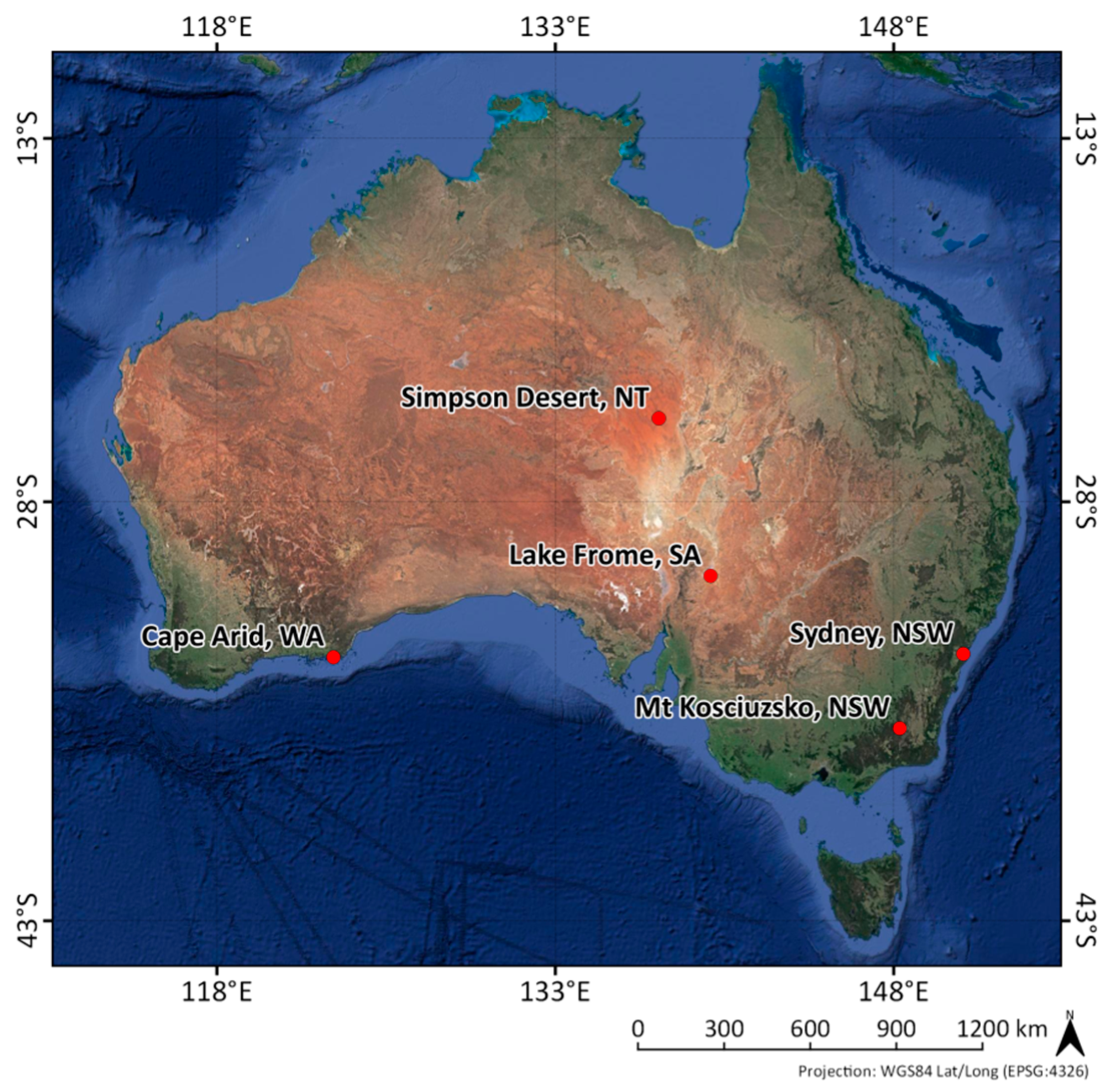
2.2. Location
The five locations chosen for analysis represent a range of different environments and land cover types (Figure 2). They include coastal, urban, desert, salt lakes, and mountainous environments.
3. Results
Results are presented in the following manner. For each of the aforementioned PQ flags (cloud and per-band saturation), one image chip per location was generated. Pixel values represent how often a given pixel was assigned a particular flag (e.g., Fmask Cloud, saturation per band) in relation to how many observations there are in total for that pixel over the course of 31 years.
3.1. Cloud Commission
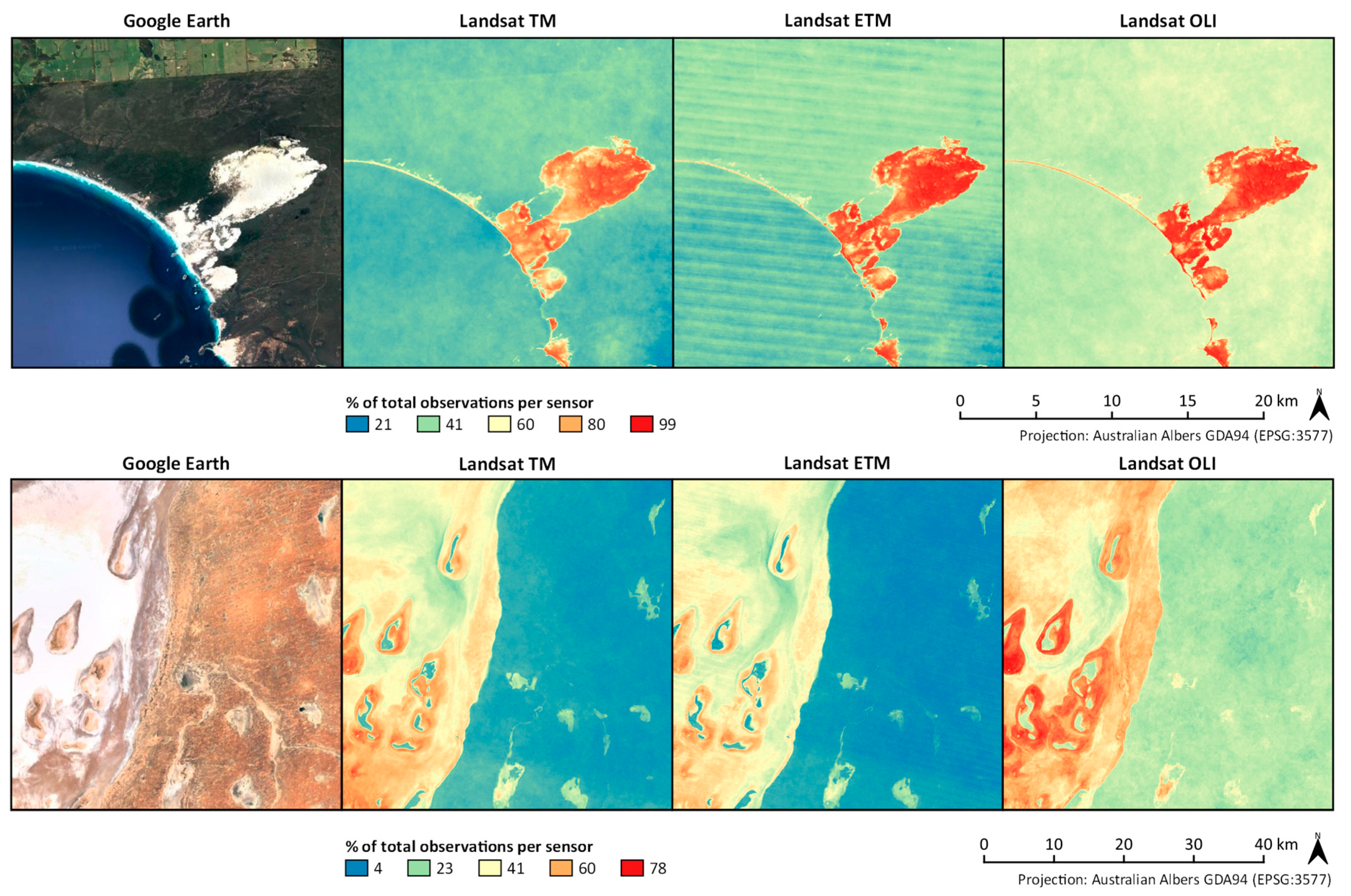
Areas featuring high rates of cloud commission errors appear to share certain characteristics. Reflectance among spectral bands was high, and similar between different bands. This was especially the case for the visible bands, making respective targets appear bright and white to the human eye. Due to high surface albedo, surface temperature in these areas was usually found to be low compared to their surroundings.
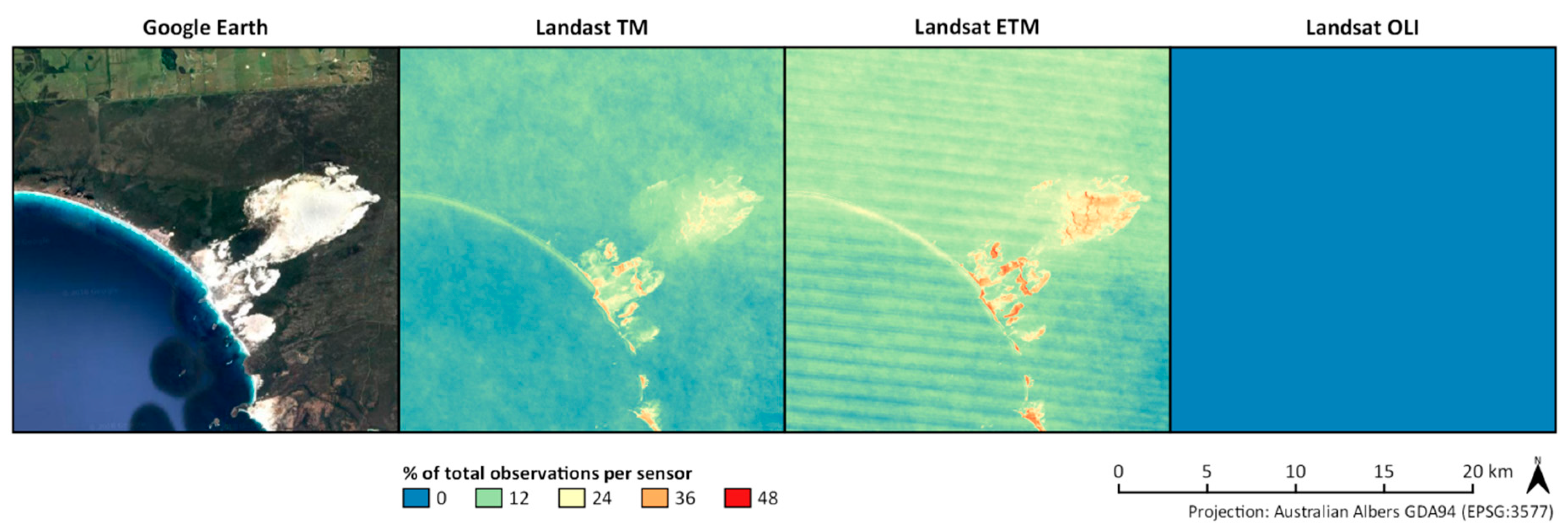
The patterns of cloud detection rates were found to be consistent across the three Landsat sensors analyzed (Figure 3). Highest Fmask cloud flag counts were found for Landsat OLI data, compared to both Landsat TM and ETM+. The uniform increase in cloud detection rate for the OLI data results from the inclusion of a cirrus band on the OLI sensor [28]. The subsequent examples are presented from a ‘whole of archive’ perspective, combining results from all sensors. This approach is taken to provide an overall view of how cloud flags are likely to impact on particular targets for tracking change over time and historical land cover changes.
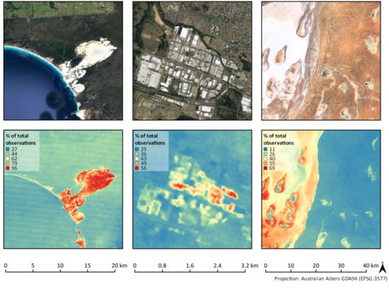
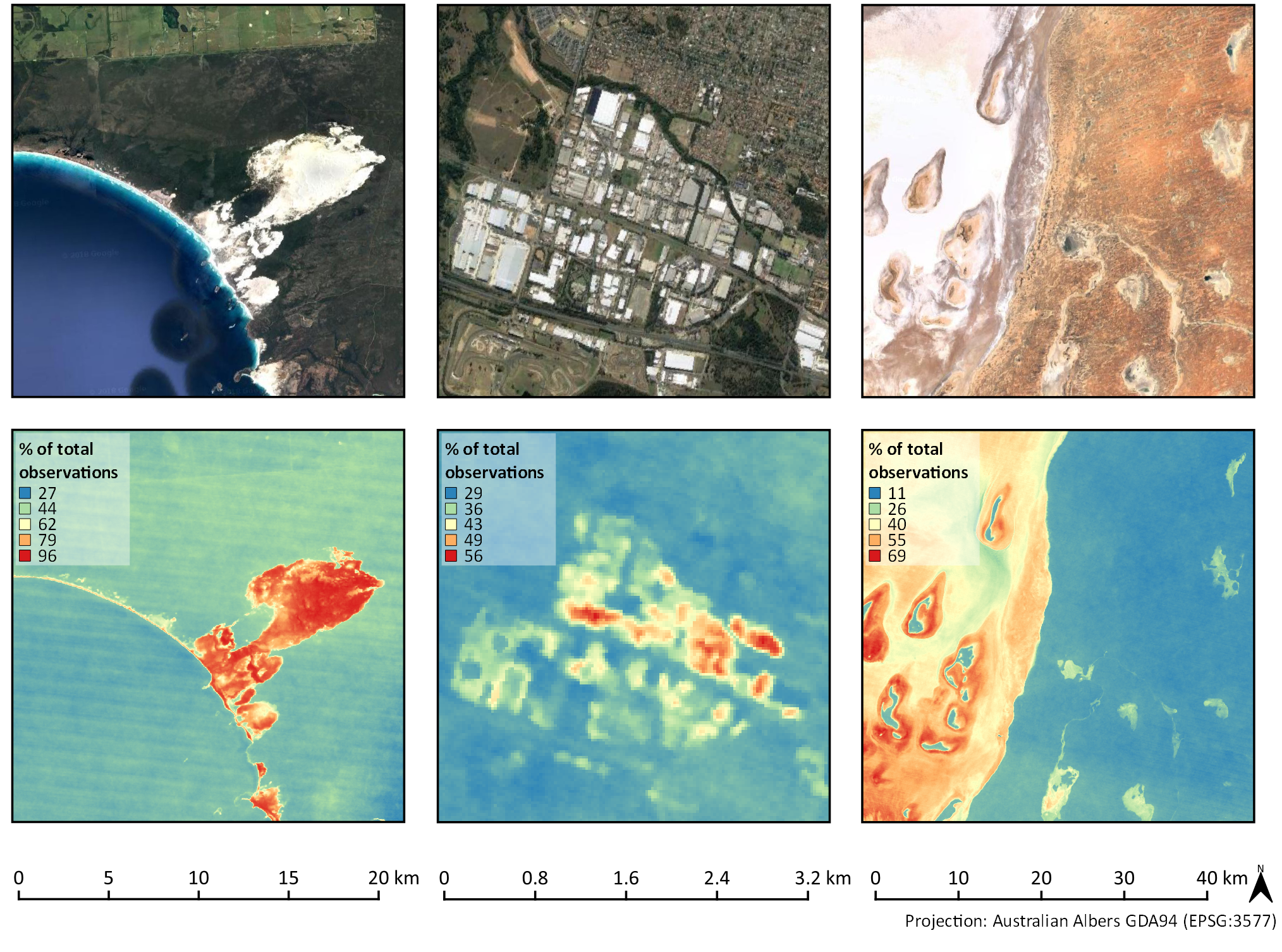
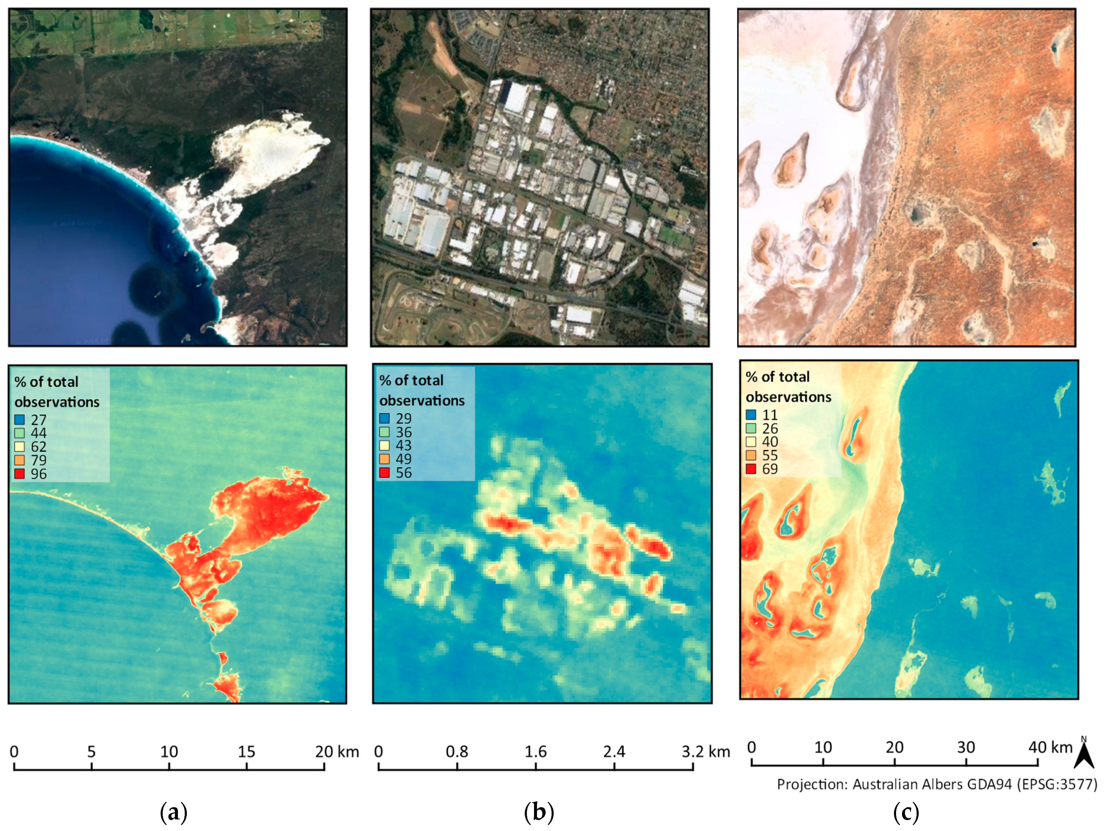
3.1.1. Coastal Areas, Urban Environments, and Salt Lakes
Beaches and sand dunes are frequently classified as cloud by Fmask. Cloud attribution rates over the sand dunes at Cape Arid shown in Figure 4a were the highest among the locations analyzed. A large part of the dunes was flagged as cloud in more than 90% of observations and beaches were frequently flagged in more than two-thirds of all observations. The remaining surface types in the image (ocean to the southwest, grassland to the north, and bushland surrounding the dune) received cloud flags in considerably fewer cases.
Certain artificial materials have the potential to frequently interfere with the accurate detection of clouds [29]. A substantial number of buildings in the Arndell Park/Huntingwood industrial area were classified for cloud; much more so than streets, vegetation patches, or residential areas to the north (Figure 4b). A comparison with historic high-resolution imagery and Landsat imagery revealed that some of the areas standing out due to high PQ cloud counts had only recently been developed. For extended periods of time between 1984 and 2016, however, these areas represented land cover types (e.g., trees, grass) that were not found to feature high cloud commission. One such example is the block to the east in Figure 3b, between the Great Western Highway and Western Motorway, which was developed past 2010. This suggests that some artificial materials can have a significant impact on cloud detection rates.
Areas covered by salt and other evaporates produce cloud commission rates that are notably higher than surrounding areas. Rates at Lake Frome appear to be highest at the fringes of salt pans, where they reach levels similar to those of the Cape Arid sand dunes (Figure 4c).
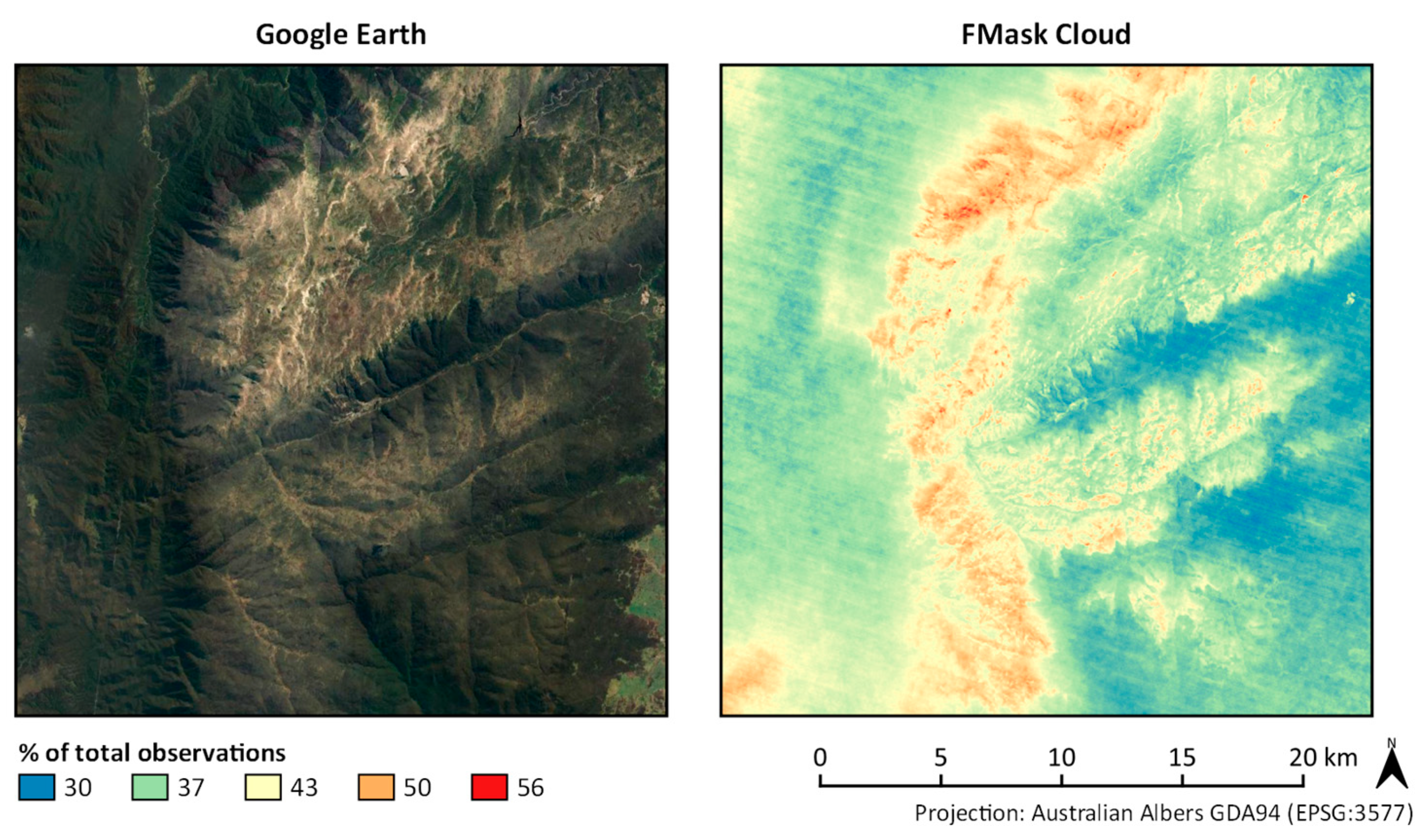
3.1.2. Mountainous/Alpine Environments
Snow and ice cover have been acknowledged to cause difficulties for Fmask [30]. We accordingly observed an increase in the number of observations flagged as cloud in mountainous areas. In the case of Mt. Kosciuszko, we observed high counts for cloud flags along the mountain ridge, while areas at lower elevation covered with vegetation were affected to a much lesser extent (see Figure 5).
3.2. Saturation
A high rate of saturation was observed for bright targets in all study sites. Surface types such as sand, barren soil, or snow/ice commonly affected observations acquired by Landsat 5 TM and Landsat 7 ETM+. Our study did not find any occurrences of saturation for Landsat 8 OLI, which indicates that increasing the radiometric resolution from 8 bit (TM and ETM+) to 12 bit (OLI) successfully addressed the issue of saturation in Landsat imagery.
While the saturation characteristics of each sensor impact their number of usable observations (Figure 6), the subsequent examples combine the results of Landsat TM, ETM, and OLI data over 31 years of data acquisition to provide insight to the characteristics of observation density that are to be expected when monitoring land cover/land use over longer periods of time.
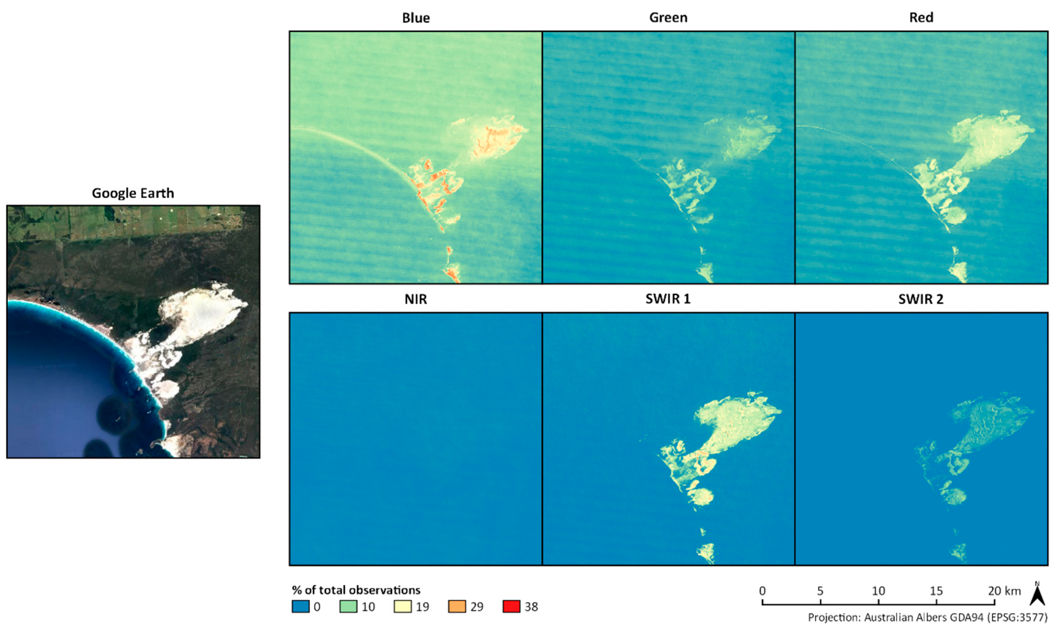
3.2.1. Coastal Environments
Saturation reduces the clear observation count over sandy beaches and sand dunes. This mainly impacts the SWIR 1 band and visible bands, while saturation in the SWIR 2 and especially the NIR band occurs less frequently (Figure 7).
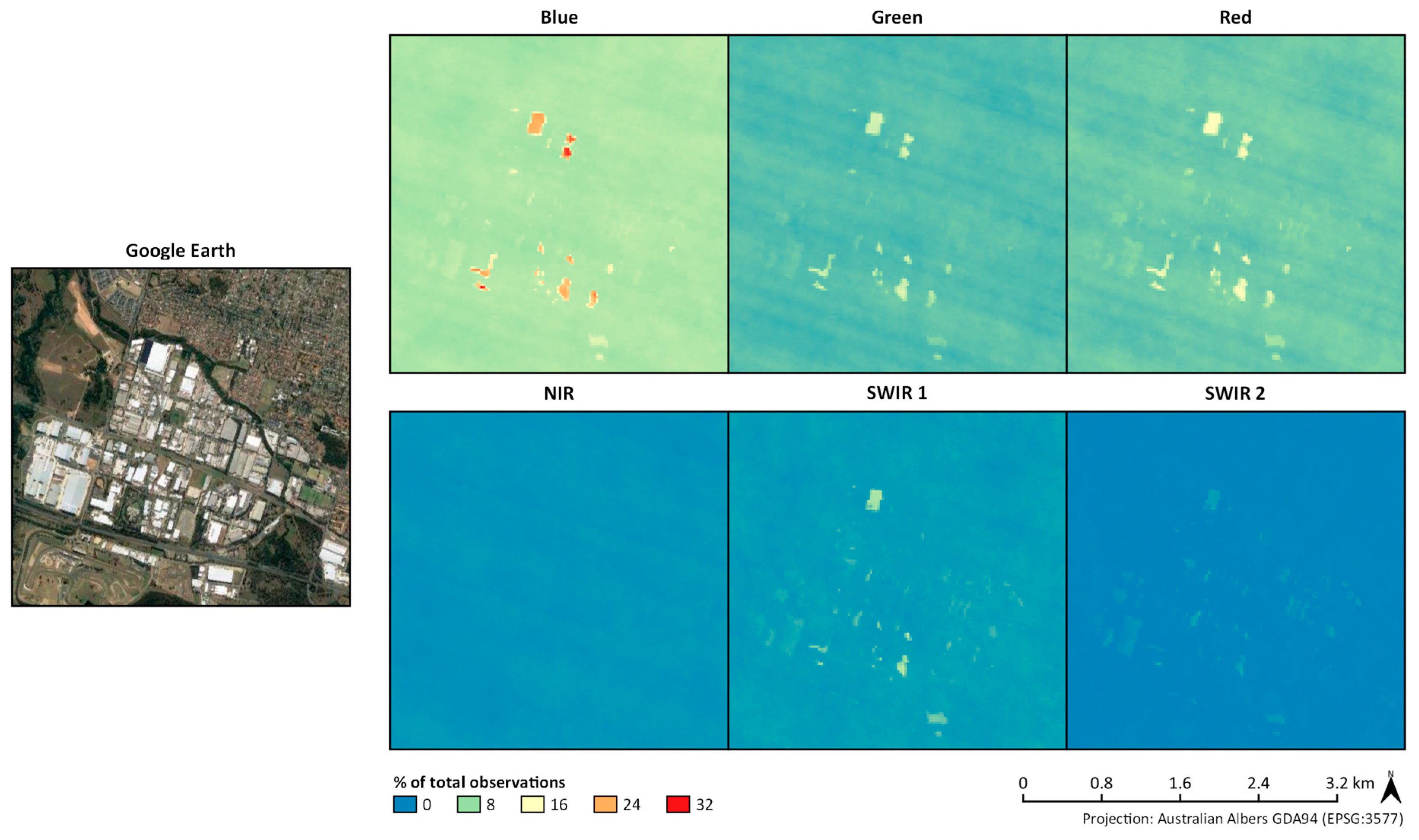
3.2.2. Urban Environments
Urban environments feature a variety of highly reflective materials. The highest saturation rates were observed in the visible bands, while the NIR band was rarely affected. The most prominent objects reducing observation count due to saturation found in the Arndell Park and Huntingwood industrial area (Figure 8) were bright roofs. The dynamic rate of change often observed in urban areas adds a level of complexity to understanding data availability or lack thereof. Based on high-resolution and Landsat imagery, we found that several structures showing high saturation rates in Figure 8 were only constructed after 2005—giving them a much shorter time window to contribute to saturation levels presented here. This suggests that saturation rates of these targets are extremely high compared to other targets that were represented in the time series for a longer period.
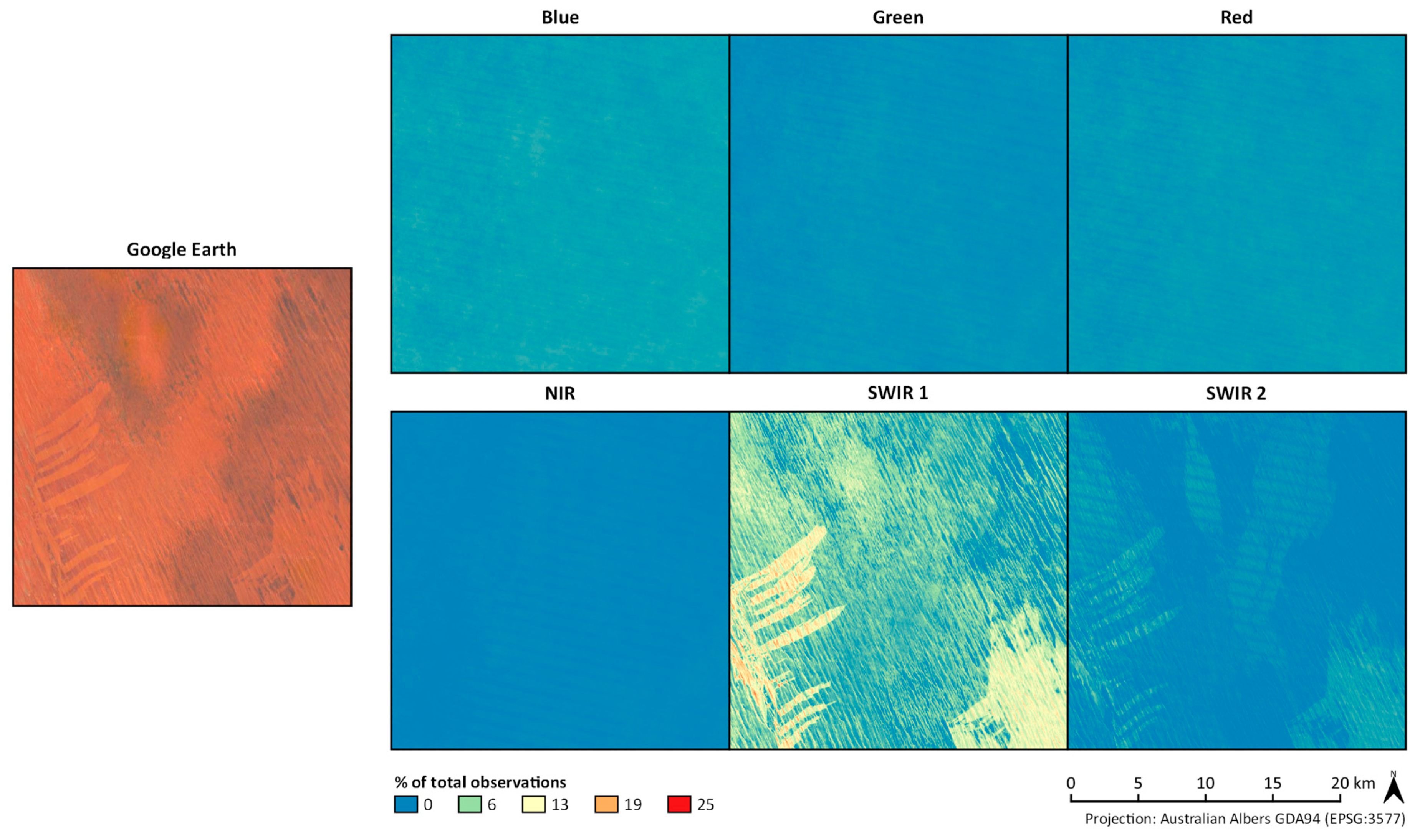
3.2.3. Deserts
Bright sand and bare rock found in Australian deserts can cause sensor saturation. Vegetation cover is often quite sparse to nonexistent, exposing underlying surface materials. Saturation in the Simpson Desert was found to predominantly occur in the SWIR bands, with visible bands and the NIR band being virtually unaffected. The structure of sand dunes is clearly visible in Figure 9 (running northwest to southeast), oriented to reflect sun towards the satellite. Even more prominent are areas in the southwest and southeast. These large stretches originate from fires burning patches of sparse vegetation, exposing bare rock and sand. The resulting burn scars are easily apparent, picked up as clear delineations in the saturation count.
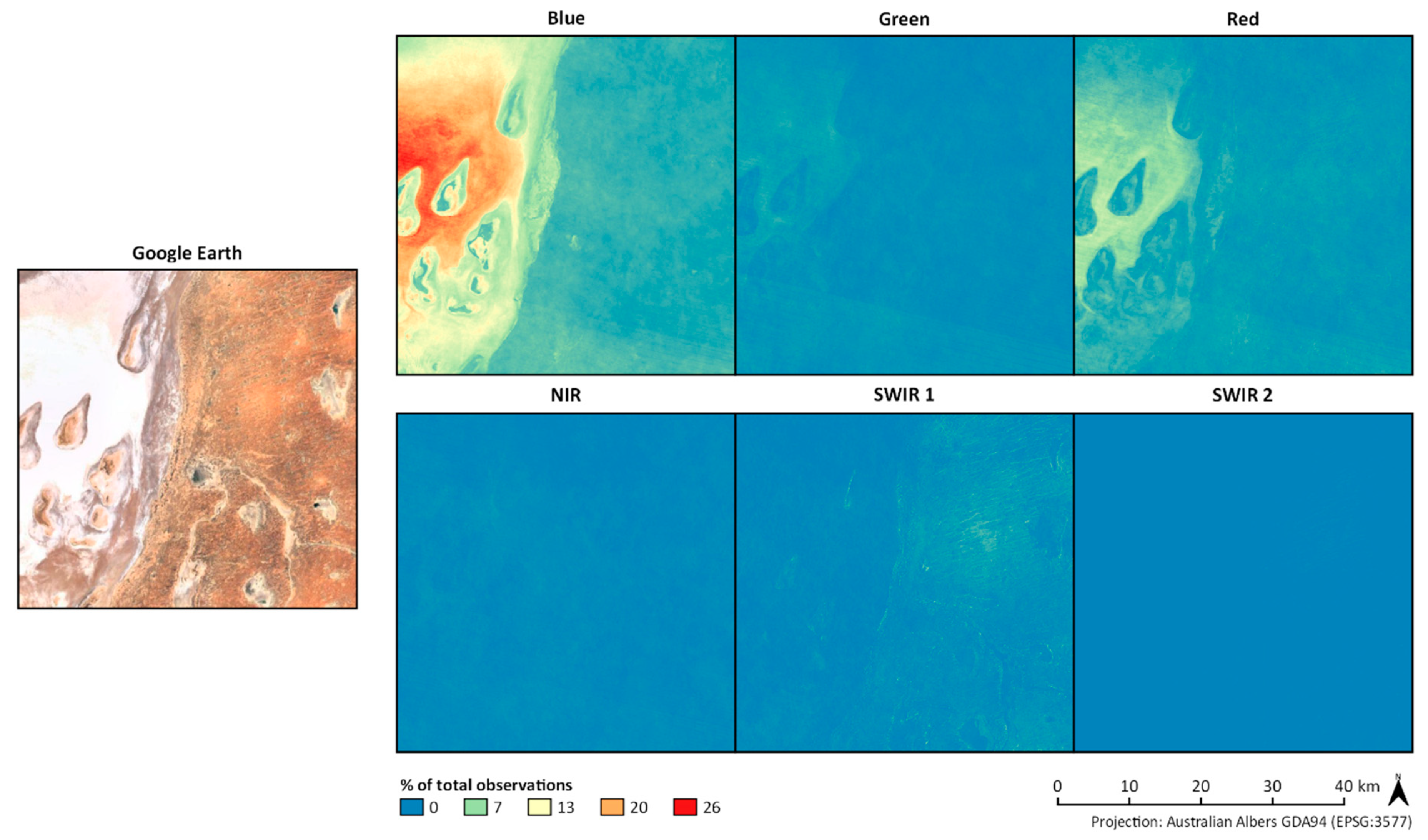
3.2.4. Salt Lakes
Stretching across more than 250,000 hectares (>640,000 acres) in remote South Australia is Lake Frome, an endorheic salt-lake. Within the salt pans of Lake Frome, saturation is most common in the blue and red bands, while the SWIR 1 band tended to saturate in the dry areas surrounding the salt-lake (Figure 10).
3.2.5. Mountainous/Alpine Environments
Moving to the opposite extreme, Australia’s highest mountain peak also left a signature on saturation rates. Standing 2228 m (7310 ft) above sea level, Mt. Kosciuszko’s snow and ice-covered summit areas frequently saturated in the visible bands. Trees may counteract saturation in lower areas due to being darker in spectral signature, as well as their shading effects on snow and ice. We found areas above the tree-line to be affected by saturation more often than areas at lower altitudes. As shown in Figure 11, the regions of Mount Kosciuszko at highest altitude clearly stand out in saturation rates.
4. Discussion and Conclusions
4.1. Cloud Screening Algorithms
This paper presents a method that allows users of ARD to evaluate the ‘fitness for purpose’ of a particular cloud screening algorithm. Fmask version 3.2 is used by way of example, as it was the most widely used cloud screening algorithm at the time when the ARD generation process for the DEA was undertaken. The algorithm has since advanced and current and future updates to Fmask may alleviate some of the cloud commission errors described in this study.
Several improvements to increase cloud detection accuracy under specific conditions have emerged for Fmask. These include updates to Fmask itself [28], but also those suggested by Frantz et al. [31] and Qiu et al. [32]. Algorithms have been designed for specific surface types or environmental conditions [14,30], as well as for sensors that lack a thermal band [28,29,31,33,34]. To overcome some of the inherent limitations of identifying cloud/cloud shadow affected pixels using the spectral characteristics of each pixel, new methods for cloud detection are being developed. These include both machine learning approaches that make use of the spatial domain [14] and multi-temporal approaches that make use of the temporal domain [18,31]. However, implementing methods that perform well across the range of surface types and environmental conditions that the Earth features is a very challenging endeavor. While the development of automated cloud screening algorithms has greatly advanced and still continues to do so, misclassification is likely to remain a challenge, especially for targets that share similar spectral characteristics with clouds. Users may wish to compare between different cloud screening approaches to identify methods that will have the least impact on their application area and analytical approach. The methods presented in this paper (counting the percentage of cloud-free observations at a particular location for a period of time) will enable users to evaluate whether these emerging cloud screening approaches are suitable for their particular region and application.
Adding further complication, pixels adjacent to clouds may become more likely to be affected by cloud shadows. Fmask and other algorithms include detection routines providing flags to indicate the presence of cloud shadow. Just as in cloud detection however, cloud shadow detection has been observed to cause errors of commission [13,19,31,32] and subsequently reduce the availability of observations. The method presented in this paper could also be used to summarize cloud shadow errors of commission.
4.2. Sensor Saturation
Sensor saturation potentially affects observations of high albedo targets in the Landsat 5 TM and Landsat 7 ETM+ components of the global Landsat archive. This issue was addressed by increasing the radiometric resolution of Landsat OLI, and we did not find any occurrences of saturation in PQ flags of OLI during our analysis. Depending on the characteristics of the observed surface type, saturation may affect a single band or multiple bands. Study designs based on spectral subsets or spectral indices may have access to an increased number of observations by excluding bands that saturate frequently in the area of interest. It is therefore desirable to have access to per-pixel information that includes saturation for each individual band during the process of screening data and designing a suitable research approach—as analyses based on spectral subsets or indices that do not include saturated bands potentially have access to an increased number of observations.
4.3. Systematic Summary of ARD
ARD is becoming more readily available, and in combination with platforms such as DEA, Google Earth Engine [35], and the Copernicus Data and Information Access Services, has the potential to greatly facilitate large-area and long-term analyses [36,37].
The availability of ARD products reduces the need for expensive preprocessing and increases transparency across different studies using the same products. While benefits are obvious, the level of customization that users can implement to extract exactly the information they need will not be the same as when preprocessing is carried out individually. It is therefore desirable that major providers of ARD deliver products with summary statistics of per-pixel QA bits to enable users to make informed analytical decisions. Based on our findings, we propose that information about atmospheric contamination (clouds) as well as per-band saturation is included in ARD products. The lack thereof may leave some applications grappling with greatly reduced data sets in some environments, or with an observation density biased towards certain surface types present in the area of interest.
Users who rely on PQ flags need to be aware of potential imbalances in observation density across space caused by saturation and cloud commission. Seasonal patterns of increasing and decreasing cloud frequency may affect the ability to detect phenologically important features. Users of ARD are advised to assess the observation density during their season/period of interest to evaluate whether this phenomenon is likely to affect their analysis. Understanding the implications of different surface types on PQ can guide the process of constructing a study design that makes best use of the available data. Great care should be taken when carrying out long-term analysis in dynamic areas such as urban environments. Targets that have been shown to affect saturation and cloud commission rates may strongly impact data availability. Like change processes themselves, each element of interference is prone to variability. Analyzing the information provided by PQ before analyzing spectral data can therefore provide appropriate insight into what limitations and biases in observation density are to be expected.
Author Contributions
L.L. and S.E. conceived and designed the experiments; S.E. performed the experiments; S.E. and L.L. analyzed the data; J.S. contributed analysis tools; S.E. and L.L. wrote the paper.
Funding
This research received no external funding.
Acknowledgments
The authors would like to thank Robbi Bishop-Taylor, Medhavy Thankappan, David Frantz, and Patrick Hostert as well as two anonymous reviewers for feedback that improved the manuscript. This research was undertaken with the assistance of resources from the National Computational Infrastructure (NCI), which is supported by the Australian Government. This paper is published with the permission of the Chief Executive Officer, Geoscience Australia.
Conflicts of Interest
The authors declare no conflict of interest.
References
- Hermosilla, T.; Wulder, M.A.; White, J.C.; Coops, N.C.; Hobart, G.W.; Campbell, L.B. Mass data processing of time series Landsat imagery: Pixels to data products for forest monitoring. Int. J. Digit. Earth 2016, 9, 1035–1054. [Google Scholar] [CrossRef]
- Hansen, M.C.; Potapov, P.V.; Moore, R.; Hancher, M.; Turubanova, S.A.; Tyukavina, A.; Thau, D.; Stehman, S.V.; Goetz, S.J.; Loveland, T.R.; et al. High-resolution global maps of 21st-century forest cover change. Science 2013, 342, 850–853. [Google Scholar] [CrossRef] [PubMed]
- Pekel, J.F.; Cottam, A.; Gorelick, N.; Belward, A.S. High-resolution mapping of global surface water and its long-term changes. Nature 2016, 540, 418–422. [Google Scholar] [CrossRef] [PubMed]
- Kennedy, R.E.; Yang, Z.; Cohen, W.B. Detecting trends in forest disturbance and recovery using yearly Landsat time series: 1. LandTrendr—Temporal segmentation algorithms. Remote Sens. Environ. 2010, 114, 2897–2910. [Google Scholar] [CrossRef]
- Zhu, Z.; Woodcock, C.E. Continuous change detection and classification of land cover using all available Landsat data. Remote Sens. Environ. 2014, 144, 152–171. [Google Scholar] [CrossRef]
- Griffiths, P.; van der Linden, S.; Kuemmerle, T.; Hostert, P. A pixel-based Landsat compositing algorithm for large area land cover mapping. IEEE J-STARS 2013, 6, 2088–2101. [Google Scholar] [CrossRef]
- Roy, D.P.; Ju, J.; Kline, K.; Scaramuzza, P.L.; Kovalskyy, V.; Hansen, M.; Loveland, T.R.; Vermote, E.; Zhang, C. Web-enabled Landsat Data (WELD): Landsat ETM+ composited mosaics of the conterminous United States. Remote Sens. Environ. 2010, 114, 35–49. [Google Scholar] [CrossRef]
- White, J.C.; Wulder, M.A.; Hobart, G.W.; Luther, J.E.; Hermosilla, T.; Griffiths, P.; Coops, N.C.; Hall, R.J.; Hostert, P.; Dyk, A.; et al. Pixel-based image compositing for large-area dense time series applications and science. Can. J. Remote Sens. 2014, 40, 192–212. [Google Scholar] [CrossRef]
- Frantz, D.; Röder, A.; Stellmes, M.; Hill, J. Phenology-adaptive pixel-based compositing using optical earth observation imagery. Remote Sens. Environ. 2017, 190, 331–347. [Google Scholar] [CrossRef]
- Mueller, N.; Lewis, A.; Roberts, D.; Ring, S.; Melrose, R.; Sixsmith, J.; Lymburner, L.; McIntyre, A.; Tan, P.; Curnow, S.; et al. Water observations from space: Mapping surface water from 25 years of Landsat imagery across Australia. Remote Sens. Environ. 2016, 174, 341–352. [Google Scholar] [CrossRef]
- Sagar, S.; Roberts, D.; Bala, B.; Lymburner, L. Extracting the intertidal extent and topography of the Australian coastline from a 28 year time series of Landsat observations. Remote Sens. Environ. 2017, 195, 153–169. [Google Scholar] [CrossRef]
- Irish, R.R. Landsat 7 Automatic Cloud Cover Assessment. Available online: https://bit.ly/2QQhiiy (accessed on 21 September 2018).
- Zhu, Z.; Woodcock, C.E. Object-based cloud and cloud shadow detection in Landsat imagery. Remote Sens. Environ. 2012, 118, 83–94. [Google Scholar] [CrossRef]
- Hughes, M.; Hayes, D. Automated detection of cloud and cloud shadow in single-date Landsat imagery using neural networks and spatial post-processing. Remote Sens. 2014, 6, 4907–4926. [Google Scholar] [CrossRef]
- Zhou, G.; Zhou, X.; Yue, T.; Liu, Y. An optional threshold with SVM cloud detection algorithm and DSP implementation. Int. Arch. Photogramm. Remote Sens. Spat. Inf. Sci. 2016, XLI-B8, 771–777. [Google Scholar] [CrossRef]
- Goodwin, N.R.; Collett, L.J.; Denham, R.J.; Flood, N.; Tindall, D. Cloud and cloud shadow screening across Queensland, Australia: An automated method for Landsat TM/ETM+ time series. Remote Sens. Environ. 2013, 134, 50–65. [Google Scholar] [CrossRef]
- Jin, S.; Homer, C.; Yang, L.; Xian, G.; Fry, J.; Danielson, P.; Townsend, P.A. Automated cloud and shadow detection and filling using two-date Landsat imagery in the USA. Int. J. Remote Sens. 2013, 34, 1540–1560. [Google Scholar] [CrossRef]
- Zhu, Z.; Woodcock, C.E. Automated cloud, cloud shadow, and snow detection in multitemporal Landsat data: An algorithm designed specifically for monitoring land cover change. Remote Sens. Environ. 2014, 152, 217–234. [Google Scholar] [CrossRef]
- Foga, S.; Scaramuzza, P.L.; Guo, S.; Zhu, Z.; Dilley, R.D.; Beckmann, T.; Schmidt, G.L.; Dwyer, J.L.; Joseph Hughes, M.; Laue, B. Cloud detection algorithm comparison and validation for operational Landsat data products. Remote Sens. Environ. 2017, 194, 379–390. [Google Scholar] [CrossRef] [Green Version]
- Chander, G.; Markham, B.L.; Helder, D.L. Summary of current radiometric calibration coefficients for Landsat MSS, TM, ETM+, and EO-1 ALI sensors. Remote Sens. Environ. 2009, 113, 893–903. [Google Scholar] [CrossRef] [Green Version]
- Bindschadler, R.; Vornberger, P.; Fleming, A.; Fox, A.; Mullins, J.; Binnie, D.; Paulsen, S.J.; Granneman, B.; Gorodetzky, D. The Landsat image mosaic of Antarctica. Remote Sens. Environ. 2008, 112, 4214–4226. [Google Scholar] [CrossRef]
- Dozier, J.; Marks, D. Snow mapping and classification from Landsat Thematic Mapper data. Ann. Glaciol. 1987, 9, 97–103. [Google Scholar] [CrossRef]
- Hall, D.K.; Chang, A.T.; Siddalingaiah, H. Reflectances of glaciers as calculated using Landsat-5 Thematic Mapper data. Remote Sens. Environ. 1988, 25, 311–321. [Google Scholar] [CrossRef]
- Karnieli, A.; Ben-Dor, E.; Bayarjargal, Y.; Lugasi, R. Radiometric saturation of Landsat-7 ETM+ data over the Negev Desert (Israel): Problems and solutions. Int. J. Appl. Earth Obs. Geoinf. 2004, 5, 219–237. [Google Scholar] [CrossRef]
- Morfitt, R.; Barsi, J.; Levy, R.; Markham, B.; Micijevic, E.; Ong, L.; Scaramuzza, P.; Vanderwerff, K. Landsat-8 Operational Land Imager (OLI) radiometric performance on-orbit. Remote Sens. 2015, 7, 2208–2237. [Google Scholar] [CrossRef]
- Sixsmith, J.; Oliver, S.; Lymburner, L. A Hybrid Approach to Automated Landsat Pixel Quality. Available online: https://bit.ly/2zAGGm4 (accessed on 28 September 2018).
- Loveland, T.R.; Dwyer, J.L. Landsat: Building a strong future. Remote Sens. Environ. 2012, 122, 22–29. [Google Scholar] [CrossRef]
- Selkowitz, D.; Forster, R. An Automated Approach for Mapping Persistent Ice and Snow Cover over High Latitude Regions. Remote Sens. 2016, 8. [Google Scholar] [CrossRef]
- Zhu, Z.; Wang, S.; Woodcock, C.E. Improvement and expansion of the Fmask algorithm: Cloud, cloud shadow, and snow detection for Landsats 4–7, 8, and Sentinel 2 images. Remote Sens. Environ. 2015, 159, 269–277. [Google Scholar] [CrossRef]
- Frantz, D.; Röder, A.; Udelhoven, T.; Schmidt, M. Enhancing the detectability of clouds and their shadows in multitemporal dryland Landsat imagery: Extending Fmask. IEEE Geosci. Remote Sens. Lett. 2015, 12, 1242–1246. [Google Scholar] [CrossRef]
- Qiu, S.; He, B.; Zhu, Z.; Liao, Z.; Quan, X. Improving Fmask cloud and cloud shadow detection in mountainous area for Landsats 4–8 images. Remote Sens. Environ. 2017, 199, 107–119. [Google Scholar] [CrossRef]
- Hagolle, O.; Huc, M.; Pascual, D.V.; Dedieu, G. A multi-temporal method for cloud detection, applied to FORMOSAT-2, VENµS, LANDSAT and SENTINEL-2 images. Remote Sens. Environ. 2010, 114, 1747–1755. [Google Scholar] [CrossRef] [Green Version]
- Gomez-Chova, L.; Amoros-Lopez, J.; Ruiz-Verdu, A.; Munoz-Mari, J.; Camps-Vails, G. Operational Cloud Screening Service for Sentinel-2 Image Time Series. Available online: https://bit.ly/2zAQGvm (accessed on 28 September 2018).
- Frantz, D.; Haß, E.; Uhl, A.; Stoffels, J.; Hill, J. Improvement of the Fmask algorithm for Sentinel-2 images: Separating clouds from bright surfaces based on parallax effects. Remote Sens. Environ. 2018, 215, 471–481. [Google Scholar] [CrossRef]
- Gorelick, N.; Hancher, M.; Dixon, M.; Ilyushchenko, S.; Thau, D.; Moore, R. Google Earth Engine: Planetary-scale geospatial analysis for everyone. Remote Sens. Environ. 2017, 202, 18–27. [Google Scholar] [CrossRef]
- Egorov, A.; Roy, D.; Zhang, H.; Hansen, M.; Kommareddy, A. Demonstration of percent tree cover mapping using Landsat Analysis Ready Data (ARD) and sensitivity with respect to Landsat ARD processing level. Remote Sens. 2018, 10. [Google Scholar] [CrossRef]
- Wulder, M.A.; Coops, N.C.; Roy, D.P.; White, J.C.; Hermosilla, T. Land cover 2.0. Int. J. Remote Sens. 2018, 39, 4254–4284. [Google Scholar] [CrossRef] [Green Version]
Figure 1.
Extracting information about how often a pixel was affected by clouds in 31 years from 1986 to 2016: For each individual Landsat observation we derive PQ flags and combine them into a PQ time series stack. This stack is then summarized as a single layer, reflecting how many times a pixel was flagged as cloud. The result is normalized by the number of total observations per pixel.

Figure 2.
Overview of the locations chosen for further analysis. Imagery: Google, Landsat/Copernicus.
Figure 2.
Overview of the locations chosen for further analysis. Imagery: Google, Landsat/Copernicus.

Figure 3.
Fmask cloud flags (in percent of total observations) for Landsat TM, ETM, and OLI for Cape Arid and Lake Frome. High-resolution imagery: Google, CNES/Airbus, TerraMetrics, DigitalGlobe.
Figure 3.
Fmask cloud flags (in percent of total observations) for Landsat TM, ETM, and OLI for Cape Arid and Lake Frome. High-resolution imagery: Google, CNES/Airbus, TerraMetrics, DigitalGlobe.

Figure 4.
Fmask cloud flags (in percent of total observations) for coastal areas (a—Cape Arid, WA), urban environments (b—Ardnell Park/Huntingwood, NSW), and salt lakes (c—Lake Frome, SA). High-resolution imagery: Google, CNES/Airbus, TerraMetrics, DigitalGlobe.
Figure 4.
Fmask cloud flags (in percent of total observations) for coastal areas (a—Cape Arid, WA), urban environments (b—Ardnell Park/Huntingwood, NSW), and salt lakes (c—Lake Frome, SA). High-resolution imagery: Google, CNES/Airbus, TerraMetrics, DigitalGlobe.

Figure 5.
High-resolution imagery (Google, CNES/Airbus, DigitalGlobe) and number of observations flagged as cloud by Fmask in percent of total observations at Mt. Kosciuzsko, NSW.
Figure 5.
High-resolution imagery (Google, CNES/Airbus, DigitalGlobe) and number of observations flagged as cloud by Fmask in percent of total observations at Mt. Kosciuzsko, NSW.

Figure 6.
Saturation characteristics of the BLUE band across the Landsat TM, ETM+, and OLI sensors at Cape Arid, WA: high-resolution imagery (Google, CNES/Airbus, TerraMetrics, DigitalGlobe) and percentage of saturation flags to total observations.
Figure 6.
Saturation characteristics of the BLUE band across the Landsat TM, ETM+, and OLI sensors at Cape Arid, WA: high-resolution imagery (Google, CNES/Airbus, TerraMetrics, DigitalGlobe) and percentage of saturation flags to total observations.

Figure 7.
High-resolution imagery (Google, CNES/Airbus, TerraMetrics, DigitalGlobe), saturation flags in the visible, NIR, and SWIR bands in percent of total observations; Cape Arid, WA.
Figure 7.
High-resolution imagery (Google, CNES/Airbus, TerraMetrics, DigitalGlobe), saturation flags in the visible, NIR, and SWIR bands in percent of total observations; Cape Arid, WA.

Figure 8.
High-resolution imagery (Google), saturation flags in the visible, NIR, and SWIR bands in percent of total observations; Arndell Park/Huntingwood, Sydney, NSW.
Figure 8.
High-resolution imagery (Google), saturation flags in the visible, NIR, and SWIR bands in percent of total observations; Arndell Park/Huntingwood, Sydney, NSW.

Figure 9.
High-resolution imagery (Google, CNES/Airbus), saturation flags in the visible, NIR, and SWIR bands in percent of total observations. Simpson Desert, NT.
Figure 9.
High-resolution imagery (Google, CNES/Airbus), saturation flags in the visible, NIR, and SWIR bands in percent of total observations. Simpson Desert, NT.

Figure 10.
High-resolution imagery (Google, DigitalGlobe, CNES/Airbus), saturation flags in the visible, NIR, and SWIR bands in percent of total observations; Lake Frome, SA.
Figure 10.
High-resolution imagery (Google, DigitalGlobe, CNES/Airbus), saturation flags in the visible, NIR, and SWIR bands in percent of total observations; Lake Frome, SA.

Figure 11.
High-resolution imagery (Google, CNES/Airbus, DigitalGlobe), saturation flags in the visible, NIR, and SWIR bands in percent of total observations; Mt Kosciuszko National Park, NSW.
Figure 11.
High-resolution imagery (Google, CNES/Airbus, DigitalGlobe), saturation flags in the visible, NIR, and SWIR bands in percent of total observations; Mt Kosciuszko National Park, NSW.

© 2018 by the authors. Licensee MDPI, Basel, Switzerland. This article is an open access article distributed under the terms and conditions of the Creative Commons Attribution (CC BY) license (http://creativecommons.org/licenses/by/4.0/).
Share and Cite
MDPI and ACS Style
Ernst, S.; Lymburner, L.; Sixsmith, J. Implications of Pixel Quality Flags on the Observation Density of a Continental Landsat Archive. Remote Sens. 2018, 10, 1570. https://doi.org/10.3390/rs10101570
AMA Style
Ernst S, Lymburner L, Sixsmith J. Implications of Pixel Quality Flags on the Observation Density of a Continental Landsat Archive. Remote Sensing. 2018; 10(10):1570. https://doi.org/10.3390/rs10101570
Chicago/Turabian StyleErnst, Stefan, Leo Lymburner, and Josh Sixsmith. 2018. "Implications of Pixel Quality Flags on the Observation Density of a Continental Landsat Archive" Remote Sensing 10, no. 10: 1570. https://doi.org/10.3390/rs10101570
Note that from the first issue of 2016, this journal uses article numbers instead of page numbers. See further details here.