Article

Mapping Cropping Practices on a National Scale Using Intra-Annual Landsat Time Series Binning

1
Geomatics Lab, Humboldt-Universität zu Berlin, Unter den Linden 6, 10117 Berlin, Germany
2
Integrative Research Institute on Transformation of Human-Environment Systems, Humboldt-Universität zu Berlin, Unter den Linden 6, 10117 Berlin, Germany
3
Earth Observation, Science, Applications & Climate Department, European Space Agency, Largo Galileo Galilei 1, 00044 Frascati (Roma), Italy
4
Department of Forest and Wildlife Ecology, University of Wisconsin, 1630 Linden Drive, Madison, WI 53726, USA
*
Author to whom correspondence should be addressed.
Remote Sens. 2019, 11(3), 232; https://doi.org/10.3390/rs11030232
Submission received: 21 December 2018 / Revised: 17 January 2019 / Accepted: 17 January 2019 / Published: 23 January 2019
(This article belongs to the Section Remote Sensing in Agriculture and Vegetation)

Abstract

:
Spatially explicit information on cropland use intensity is vital for monitoring land and water resource demands in agricultural systems. Cropping practices underlie substantial spatial and temporal variability, which can be captured through the analysis of image time series. Temporal binning helps to overcome limitations concerning operability and repeatability for mapping large areas and can improve the thematic detail and consistency of maps in agricultural systems. We here assessed the use of annual, quarterly, and eight-day temporal features for mapping five cropping practices on annual croplands across Turkey. We used 2403 atmospherically corrected and topographically normalized Landsat Collection 1 L1TP images of 2015 to compute quarterly best-pixel composites, quarterly and annual spectral-temporal metrics, as well as gap-filled eight-day time series of Tasseled Cap components. We tested 22 feature sets for binary cropland mapping, and subsequent discrimination of five cropping practices: Spring and winter cropping, summer cropping, semi-aquatic cropping, double cropping, and greenhouse cultivation. We evaluated area-adjusted accuracies and compared cropland area estimates at the province-level with official statistics. We achieved overall accuracies above 90%, when using either all quarterly features or the eight-day Tasseled Cap time series, indicating that temporal binning of intra-annual image time-series into multiple temporal features improves representations of cropping practices. Class accuracies of winter and spring, summer, and double cropping were robust, while omission errors for semi-aquatic cropping and greenhouse cultivation were high. Our mapped cropland extent was in good agreement with province-level statistics (r2 = 0.85, RMSE = 7.2%). Our results indicate that 71.3% (±2.3%) of Turkey’s annual croplands were cultivated during winter and spring, 15.8% (±2.2%) during summer, while 8.5% (±1.6%) were double-cropped, 4% (±1.9%) were cultivated under semi-aquatic conditions, and 0.32% (±0.2%) was greenhouse cultivation. Our study presents an open and readily available framework for detailed cropland mapping over large areas, which bears the potential to inform assessments of land use intensity, as well as land and water resource demands.

Graphical Abstract

1. Introduction

Growing pressure on agricultural systems under rising requirements for sustainable production results in a growing need for land use intensity and land management datasets [1]. Spatially explicit information on land use intensity is crucial for tracking resource demands in the nexus of land, water, and food over space and time [2]. It is, therefore, crucial to develop mapping approaches that move beyond broad representations of cropland extent towards enabling the distinction of management-driven cropland use intensity [3,4]. Better information on the areal extent and spatial distribution of cropping practices across large areas improves the estimation of current and future land and water resource demands [5,6,7].
The strong spatio-temporal variability of croplands and irregular clear-sky image acquisitions for optical data pose challenges for robust mapping of annual cropping practices [8]. Mapping efforts thus frequently relied on coarse-resolution imagery such as MODIS or AVHRR (500 m–8 km), for instance, in the context of cropping intensity [6,9,10] or irrigation [11,12]. Landsat(-like) medium spatial resolution data (10–30 m) represent cropland management more accurately [4,13], specifically in small-holder cropping systems [9]. Consequently, a variety of studies recently improved the remote-sensing-based characterization of cropland management practices, such as irrigation [14,15,16], field sizes [17], or selected crop types [18]. However, many studies target regional characterization of single management indicators, while large area mapping efforts trying to characterize various management practices remain scarce [4].
Major challenges for mapping cropping practices with medium resolution sensors stem from low revisit frequencies and resulting sparse and irregular observation densities. The Landsat sensor family has a nominal repeat frequency of 16 days at nadir. During times with two operational satellites, repeat coverage can be up to eight days, which can, however, be spatially and temporally fragmented, e.g., due to the failure of Landsat 7’s scan line corrector [19] or changes in long-term acquisition plans [20]. Higher repeat frequency can occur in lateral overlaps of two orbits [21]. However, cloud contamination largely reduces data availability on a pixel-level [22], limiting the large-scale applicability of traditional classification approaches, which relied on a manual selection of cloud-free single or multi-date imagery. Deriving temporally aggregated, (e.g., seasonal or annual) features from Landsat image time series can help to overcome such issues, and aid in improving the thematic detail, consistency, and quality of maps in agricultural systems [23,24,25]. Common techniques to generate standardized gap-free spectral features include pixel-based compositing [26,27,28], the computation of spectral-temporal metrics [29,30,31], as well as data fusion [32,33] or gap-filling techniques [34]. Such temporal features can be produced consistently for multiple periods and large areas [35]. Furthermore, they contain information on land surface phenology, which renders them suitable for mapping cropping practices across gradients of climate, topography, or land use intensity [36].
Land-surface phenology on annual croplands is particularly heterogeneous and dynamic, due to a variety of management-regimes. In water-scarce regions, for instance, growing cycles of cultivated lands are largely precipitation-driven. However, irrigation locally decouples cropland cultivation from precipitation-based restrictions in water availability. Consequently, the timing and amplitude of growing cycles of irrigated lands strongly deviate from the phenological cycles of rainfed crops [36,37]. Identifying the timing of phenological events relevant for characterizing different cropland management practices is a challenging task [38] and requires either regional expert knowledge or data-driven approaches to identify key phenological events in a spatially explicit manner [39]. This problem is further aggravated in the case of large area mapping, where diverse management regimes control for additional heterogeneity in the timing and number of growing cycles, as opposed to natural ecosystems, where climate or topography are primary drivers of shifts in phenology [27]. Additionally, the inter-annual variability of cropland management decisions, such as crop rotations, prohibits data pooling across multiple years, as can be used in more persistent environments such as forested ecosystems [40,41].
Turkey has been, and is, undergoing policy-driven agricultural intensification. In this context, land consolidation efforts increased productivity by reducing parcel fragmentation across the country [42], and the expansion of irrigation infrastructure fostered regional development through increased agricultural production [43]. On the one hand, these policies boosted crop production over decades, ranking Turkey amongst the world’s leading producers of cereals and other industrial crops [44]. On the other hand, they also resulted in a diverse agricultural landscape, dispersed along gradients in climate and topography, with a strong inter-annual variability in management practices [45]. Furthermore, low irrigation water use efficiencies [44,45], as well as the limited availability of land and water resources require optimization of cropland management towards a higher resource use efficiency. In this context, spatially explicit data on cropping practices is of high value to understand past and current patterns and drivers of land use intensity and associated resource consumption.
Growing information needs demand for accessible and operational methodologies, and analysis-ready data (ARD), defined as cloud-screened surface reflectance products delivered in regular tiles [46], or higher level time-series products [47]. Such data can enable large area cropland management mapping, independent of costly calibration efforts, which rely on ancillary ground data or large area characterization of vegetation phenology [4]. The Landsat archive is the longest uninterrupted global satellite dataset and thus provides an accessible and consistent data basis for deriving such information. In this study, we compare different approaches for Landsat time-series aggregation. We used consistently produced Landsat Collection 1 data and openly available processing frameworks for generating ARD to promote readily applicable data and methods for large area mapping at medium spatial resolution. The key aim of this paper is to present a set of scientifically sound and openly accessible good practice recommendations for operational national scale mapping of cropland use intensity, demonstrated using the case of mapping cropping practices across Turkey. Specifically, our objectives are to:
  • Test the performance of Landsat time-series binning methods for mapping cropping practices on annual croplands in Turkey.
  • Investigate the spatial patterns of cropping practices across Turkey.
  • Compile a set of good practice recommendations for Landsat-based mapping of cropping practices over large areas.

2. Materials and Methods
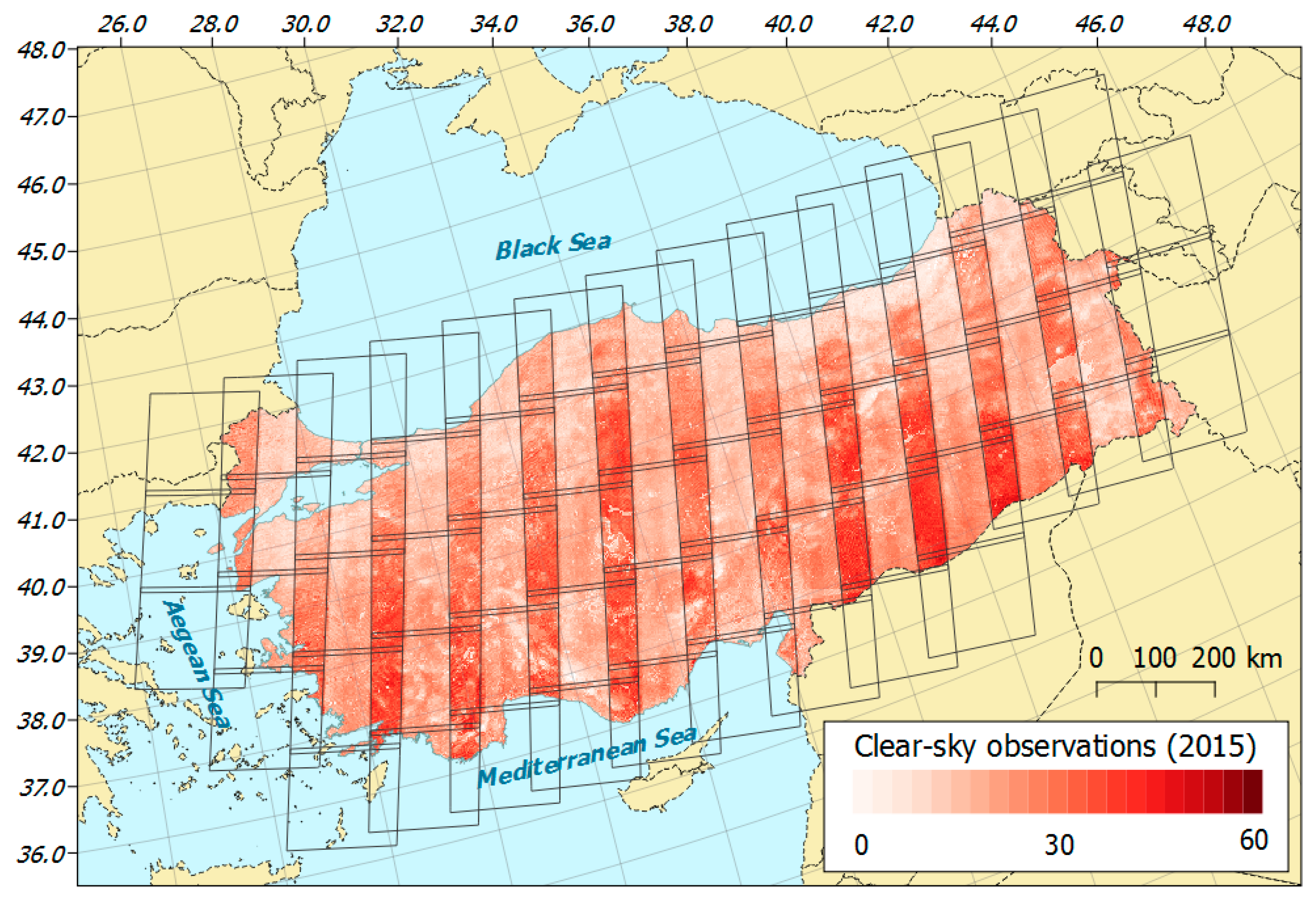
2.1. Study Area

Located at the intersection of the European and Asian continent, Turkey’s geopolitical role in agricultural production and trade has persisted through centuries. Turkey covers an area of 783,000 km2. To date, roughly one-third of the country’s land is cultivated [45]. Due to strong biophysical and cultural gradients, Turkey’s agricultural lands comprise nine distinct agro-ecosystems that differ in biophysical characteristics, crop types, and cropping practices [45]. In 2015, Turkey’s cultivated lands included 15.7 Mha of annual cropland, plus an additional 4.1 Mha of temporary fallow land [48]. Cereals represent nearly two-thirds of the harvested land in Turkey, most notably wheat (35%), barley (12%), and maize (10%) [48]. Additionally, sugar beets (25%), potatoes (7%), sunflower (3%), cotton (3%), and pulses (2%) are grown. As extensive parts of the country have semi-arid to arid climate, irrigation is key for economically viable agricultural production [44]. Rainfed cultivation during spring and the first summer months is possible in most parts of the country. Contrarily, cultivation during the dry summer months requires irrigation for successful crop development in the water-limited regions of Turkey, like Central and South-Eastern Anatolia. Summer cropping in these regions is indicative of irrigation [49]. Irrigation is widespread and currently present on 4.9 Mha, being subject to further expansion and projected to reach 8.5 Mha by 2030 [45]. Seventy-eight percent of the irrigated land is irrigated with surface water, which is mostly applied through surface irrigation (92%), followed by sprinkler (6%) and drip (2%) irrigation [45]. However, national water use efficiency was below 50%, causing substantial water losses [45]. Furthermore, up to 55% of the area equipped for irrigation was not irrigated on an annual basis due to mismanagement, water shortages, and institutional barriers at the local level, reflecting underused investments into irrigation infrastructure [44], which can cause strong spatio-temporal dynamics of rainfed and irrigated cropping, and thus to a high variability in land use intensity.

2.2. Data Pre-Processing and Class Catalogue

We downloaded 1143 Landsat 7 ETM+ and 1269 Landsat 8 OLI images for the year 2015 that cover our study area of 63 WRS-2 scenes. As we aimed for achieving high radiometric and geometric consistency, we used exclusively Landsat Collection 1 Level 1 Tier 1 precision terrain corrected (C1 L1TP T1) images with a cloud cover of less than 80%. For conversion into topographically normalized surface reflectance, we performed atmospheric correction and topographic normalization using a modified C-correction for topographic normalization to avoid topography-driven misclassification [50,51]. Generation of ARD, i.e., cloud and cloud shadow masking, radiometric correction (atmospheric, topographic, BRDF and adjacency effect correction), and data cubing (reprojection to ETRS89-LAEA projection and tiling into a 30 km × 30 km grid) were performed with the Framework for Operational Radiometric Correction for Environmental Monitoring (FORCE v. 1.1, freely available at http://force.feut.de), based on the algorithm described in Reference [52].
For classification, we included several auxiliary features. We used the 1 Arc-Second (~30 m) digital elevation model acquired by the Shuttle Radar Topography Mission [53] to derive elevation and hillslope. Additionally, we generated per-pixel latitude and longitude in geographic coordinates to account for large-scale variability in land cover characteristics.
We used a hierarchical class definition, first distinguishing annual cropland from other land cover and land use classes. In a next step, we classified annual croplands into five distinct classes of cropping practices, which characterize the annual cropland system of Turkey and relate to its use intensity (Table 1). The hierarchical approach enables the evaluation of the cropping practice maps independently of the respective cropland mask used. The areal extent of the cropping practice classes was expected to vary strongly. While wheat production in Turkey covers extensive areas, greenhouse cultivation only accounts for a marginal share of the cropland area [45,48]. Accurately capturing small classes in large area mapping poses additional challenges related to training data collection and validation [54]. However, due to our objective to characterize the annual crop production system in a holistic manner, as well as the relevance of classes like semi-aquatic cropping and greenhouse cultivation regarding land and water resource consumption, we decided to integrate these classes in our class catalog. Examples of the spectral-temporal dynamics of our target classes are available in Appendix B.

2.3. Generation of Temporal Features

We used all available clear-sky observations (CSO) for temporal binning of all images into gap-filled eight-day, quarterly, and annual temporal features. While previous studies relied on annual temporal binning, we here introduced the quarterly binning as an intermediate trade-off between a high temporal resolution and an observation availability, which is sufficient for producing near gap-free coverage. The gap-filled eight-day temporal window represents an ideal case, where clear observations are available on a near-weekly basis. We derived temporally aggregated features using time-series gap filling, best-observation compositing, as well as the computation of spectral-temporal metrics. All higher-level products were generated using FORCE v.1.1.

2.3.1. Best-Observation Composites

We used 2403 atmospherically corrected and topographically normalized, cloud-screened Landsat Collection 1 L1TP T1 images to compute four best-observation composites [26] across Turkey. To identify the best observation, we conducted a parametric scoring which considered the temporal distance to the target day of the year, as well as the distance to clouds and cloud shadows and a haze score as parameters [27]. We used all available imagery from each quarter of 2015 to produce composites for the target days 15 February, 17 May, 16 August, and 16 November for the blue, green, red, near infrared, and both shortwave infrared bands, summing up to 24 features.
For quality checking and interpretation, we derived compositing flags containing information on the quality, number of CSOs per pixel, the acquisition date of the best observation, the difference between the acquisition date and target day of the year (DOY), as well as the sensor. Additionally, we computed the CSO count for the entire year, considering all areas free of clouds, cloud shadows, snow, and ice, which were not compromised by radiometric saturation.

2.3.2. Spectral-Temporal Metrics

We generated eleven band-wise spectral-temporal metrics for each quarter and the entire year using the CSOs available in the respective period. We computed the minimum, 25th percentile, median, 75th percentile, and maximum, mean spectral reflectance as well as the inter-quartile-range, range, and standard deviation of all reflectance values during each period. Additionally, we calculated the skewness and kurtosis of the distribution of reflectance values in the respective period. In total, the eleven spectral-temporal metrics for each quarter and spectral band sum up to 264 quarterly features, plus 66 spectral-temporal metrics from all observations of 2015.

2.3.3. Equidistant Time Series of Tasseled Cap Components

The Tasseled Cap transformation represents a linear transformation of the Landsat spectral bands into components which express selected physical scene characteristics [55]. We applied the Tasseled Cap transformation based on the coefficients for Landsat surface reflectance [56] on the CSOs to generate an equidistant eight-day interval time series of the Tasseled Cap Brightness, Greenness, and Wetness components. We used a data-density weighted ensemble of three Radial Basis Function (RBF) convolution filters for smoothing and gap-filling of the time series [34]. We chose to produce a time series of three Tasseled Cap components over a time series of standard vegetation indices since the Tasseled Cap transformation integrates the entire spectral information content of the six Landsat bands. While the vegetation signal is emphasized by the Tasseled Cap greenness component, the Tasseled Cap wetness, and brightness components potentially aid in the classification of our target classes such as semi-aquatic croplands and greenhouses.
The RBF approach is an ensemble technique, which combines multiple kernels to reduce noise and outliers in a time series while enabling to capture the variability of the signal in managed systems. We defined an ensemble of Gaussian kernels with σ1 = 8, σ2 = 16, and σ3 = 32 days, respectively and applied a kernel-cutoff parameter that restricted the absolute width of the Gaussian kernels to ±21, 41, and 82 days relative to the target date. These kernels are relatively narrow compared to previous studies with a focus on natural ecosystems [34] and provide a trade-off between data gap reduction and the description of dynamic events, such as harvests. We finally aggregated the three kernels by calculating a data-density weighted mean, which gives preference to kernels with a higher data density for the final estimation.
The procedure resulted in a near gap-free eight-day time-series of three Tasseled Cap components for the year 2015, which consisted of 135 features. We further calculated the mean, standard deviation, minimum, and maximum of the Brightness, Greenness, and Wetness time series for the entire year, resulting in 12 additional features.

2.4. Training Data & Classification

We collected training polygons with a minimum extent of nine pixels (0.8ha), using the composites, an Enhanced Vegetation Index (EVI) time series for the years 2014–2016 (produced following the methods for the Tasseled Cap time series), and high-resolution imagery available in Google Earth. We collected 1925 training polygons in the different agricultural regions, comprising the Middle North, Aegean, Thrace, Mediterranean, Northeast, Southeast, Black Sea, Middle East, and Middle South regions [45], to capture the heterogeneous management regimes across Turkey. We reduced the number of training samples to 15% of the pixels in each polygon, with a minimum of two and a maximum of 30 pixels, resulting in 10,340 training points (of which 50.2% represented annual croplands).
We compiled 22 different subsets of the 505 input features (Table 2). We categorized the feature subsets based on the employed temporal binning. The annual scheme refers to annual spectral-temporal metrics, combinations of composites and spectral-temporal metrics from all quarters of the year, all quarterly composites, all quarterly spectral-temporal metrics, or annual statistics derived from the Tasseled Cap time series. The bi-quarterly scheme refers to six combinations of two quarterly composites and spectral-temporal metrics; whereas the quarterly feature sets include composites and spectral-temporal metrics from one quarter only. For the quarterly and annual scheme, we further combined all quarterly feature subsets with annual spectral-temporal metrics. For the weekly scheme, we used the eight-day time series of Brightness, Greenness, and Wetness, as well as the time series together with the annual Tasseled Cap statistics. We used Random Forest classification models [57] for classification of each feature subset using n = 500 trees and included the square root of the number of features at each split. This procedure was used to separately produce binary cropland maps, as well as cropping practice maps for the study region.

2.5. Validation Data & Accuracy Assessment

Assuming user’s accuracies of 0.85 for all classes and targeting a standard error of the overall accuracy of 1% regarding binary cropland mapping and 2% for the cropping practice mapping, we determined a required sample size of 1275 for the binary and 391 for the cropping practices map, respectively [58]. We performed a stratified allocation of the reference samples due to high imbalances in the extent of specific land uses. We produced a preliminary classification based on all quarterly spectral-temporal metrics and composites, which represented the five cropping practice classes plus nine sub-classes not related to annual croplands. This map provided the strata for implementing a stratified random sampling, allowing us to allocate samples in diverse types of non-cropland areas, such as grasslands, shrublands, or urban environments. We calculated the confidence intervals of accuracies and area estimates for four different sample allocation schemes and determined an allocation scheme with a class-wise minimum of 50 samples, and the remainder was distributed according to class weights derived from the preliminary map as a suitable allocation [54]. The final sample comprised 1447 validation points, 465 of which were annual cropland samples (166 samples for winter cropping: 106 for summer cropping, 63 for semi-aquatic cropping, 67 for double cropping, and 63 for greenhouse cultivation).
We pre-compiled relevant information for each validation point, containing image chips of pixel-based composites displayed in false-color RGB at three different zoom levels, pixel spectra of the point locations, and an EVI time series spanning 2014–2016 (see Appendix B for examples). Based on this phenological information, we determined the class label for each validation sample. We further considered the pixel extent of each sample in Google Earth to verify the label against high-resolution imagery from 2015, or the closest acquisition year available. This was particularly useful to increase the certainty for separating cropland from grassland and for identifying greenhouses. Two trained interpreters crosschecked 25% of the samples, finding interpreter agreement in more than 95% of all cases. Reference points where class labels could not be determined with high confidence were removed. We predicted the reference data points for each classification model and computed area-adjusted overall accuracies as well as area-adjusted class accuracies [54].

3. Results

3.1. Clear Sky Observation Density

We registered an average of 20.42 CSOs per pixel (minimum 0; maximum 62) during the study period. A spatially explicit visualization of CSOs (Figure 1) revealed data-scarce areas in the Eastern parts of the Black Sea region, while observation density in the across-track overlap areas in South Eastern Anatolia (southeast Turkey, alongside the Syrian border) was the highest. Time windows covering single quarters of the year showed few gaps, except for the first quarter, where 9% of the study area remained unobserved (Table 3).

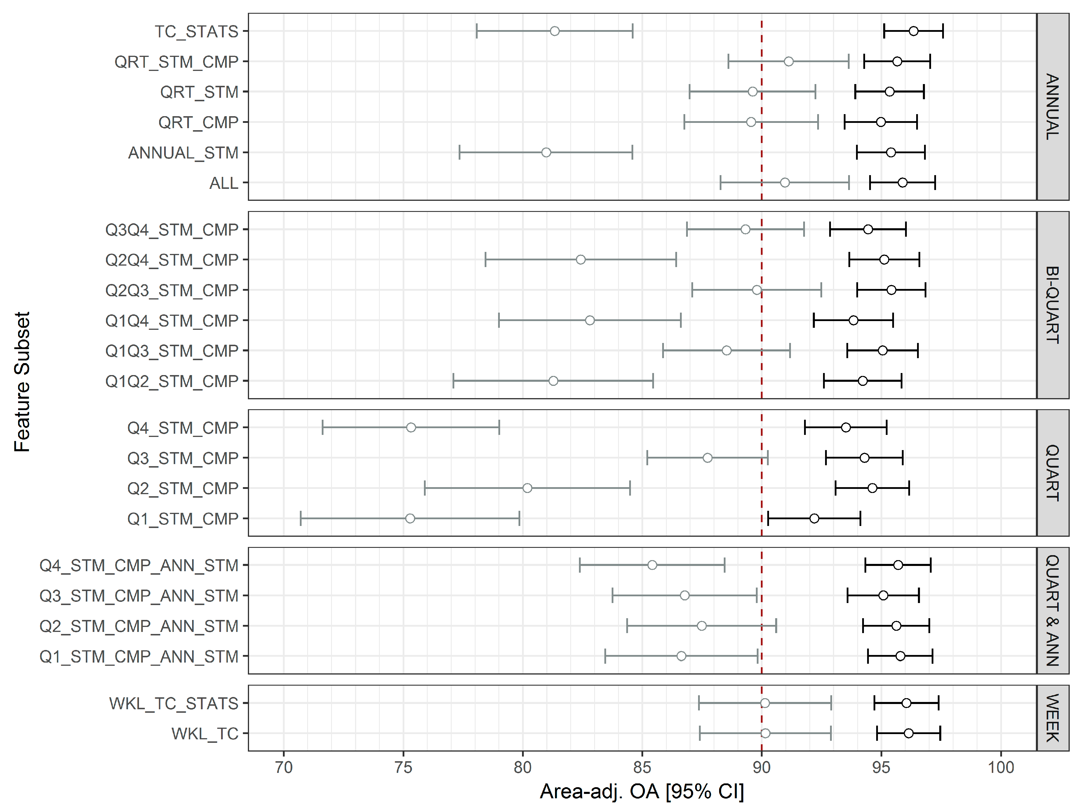
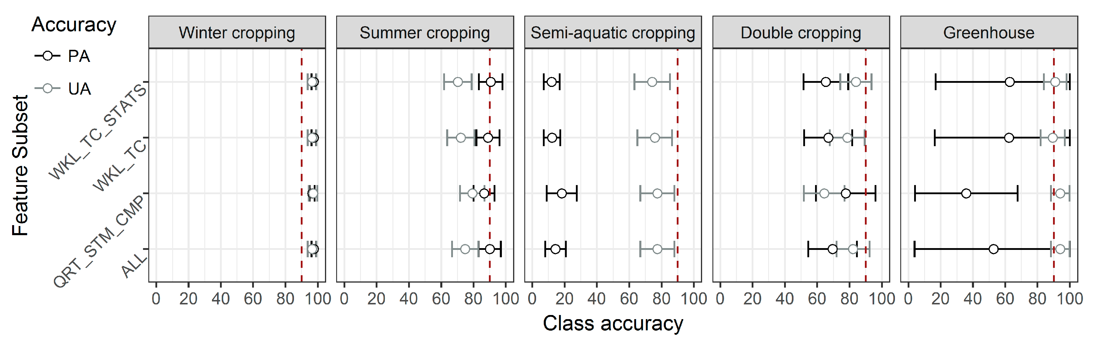
3.2. Classification Accuracies

We calculated the area-adjusted overall accuracies as well as their 95% confidence intervals for each binary cropland and cropping practice classification for all 22 input feature sets. The binary classification was robust (Figure 2, black signature) with overall accuracies exceeding 92% throughout, whereas variations in accuracy values were apparent for the cropping practice classification (Figure 2, grey signature).
Generally, features generated from annual data outperformed the seasonally restricted approaches, while the low accuracies of TC_STATS and ANNUAL_STM suggest that retaining seasonal information in temporal aggregates through seasonal binning is essential. We found no differences in overall accuracy when using only composites or only spectral-temporal metrics. Combining both, however, improved the overall accuracy. In the category of bi-quarterly inputs, involving data from the spring and summer months, performed well. Similarly, the single-quarter classifications showed that spectral-temporal metrics and composites from the summer quarter were sufficient for achieving overall accuracies above 85%. Using spectral-temporal metrics and composites from the data-scarce first and fourth quarters, however, yielded the lowest accuracies. Adding feature sets from other seasons generally increased accuracy. Including geographic location (latitude, longitude) and topography (elevation, slope) as auxiliary variables increased the overall accuracies by 1%–3% throughout, indicating their benefit for large area mapping.
Four models exceeded 90% overall accuracy in both binary cropland and cropping practice mapping (Table A1, Table A2, Table A3 and Table A4). These were ALL (all features), QRT_STM_CMP (quarterly composites and spectral-temporal metrics), WKL_TC (eight-day time series of three Tasseled Cap components), and WKL_TC_STATS (eight-day time series of three Tasseled Cap components complemented with four annual statistics). All these feature sets retain temporal information throughout the different seasons. Class wise user’s and producer’s accuracies of these four best models showed robust mapping of spring and winter cropping, summer cropping, and double cropping, whereas semi-aquatic cropping and greenhouse cultivation showed low producer’s accuracies (Figure 3).
We based the following analyses on model WKL_TC_STATS, because the cropland extent was closest to official statistics (see Section on Cropland Area Estimates), and the spatial consistency was found to be the highest.

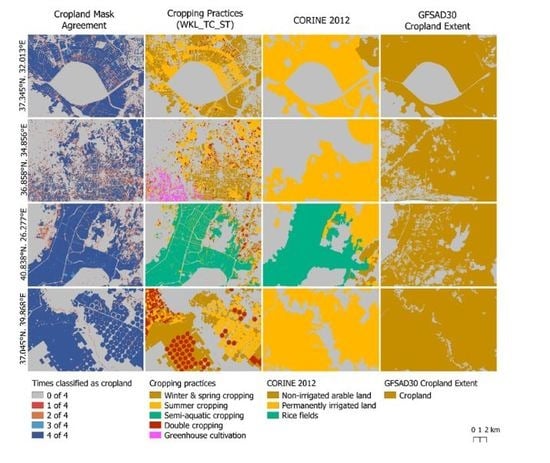
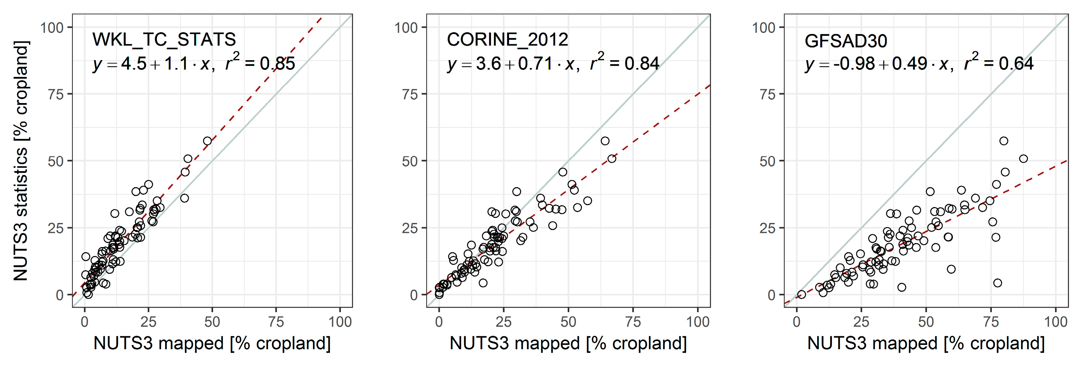
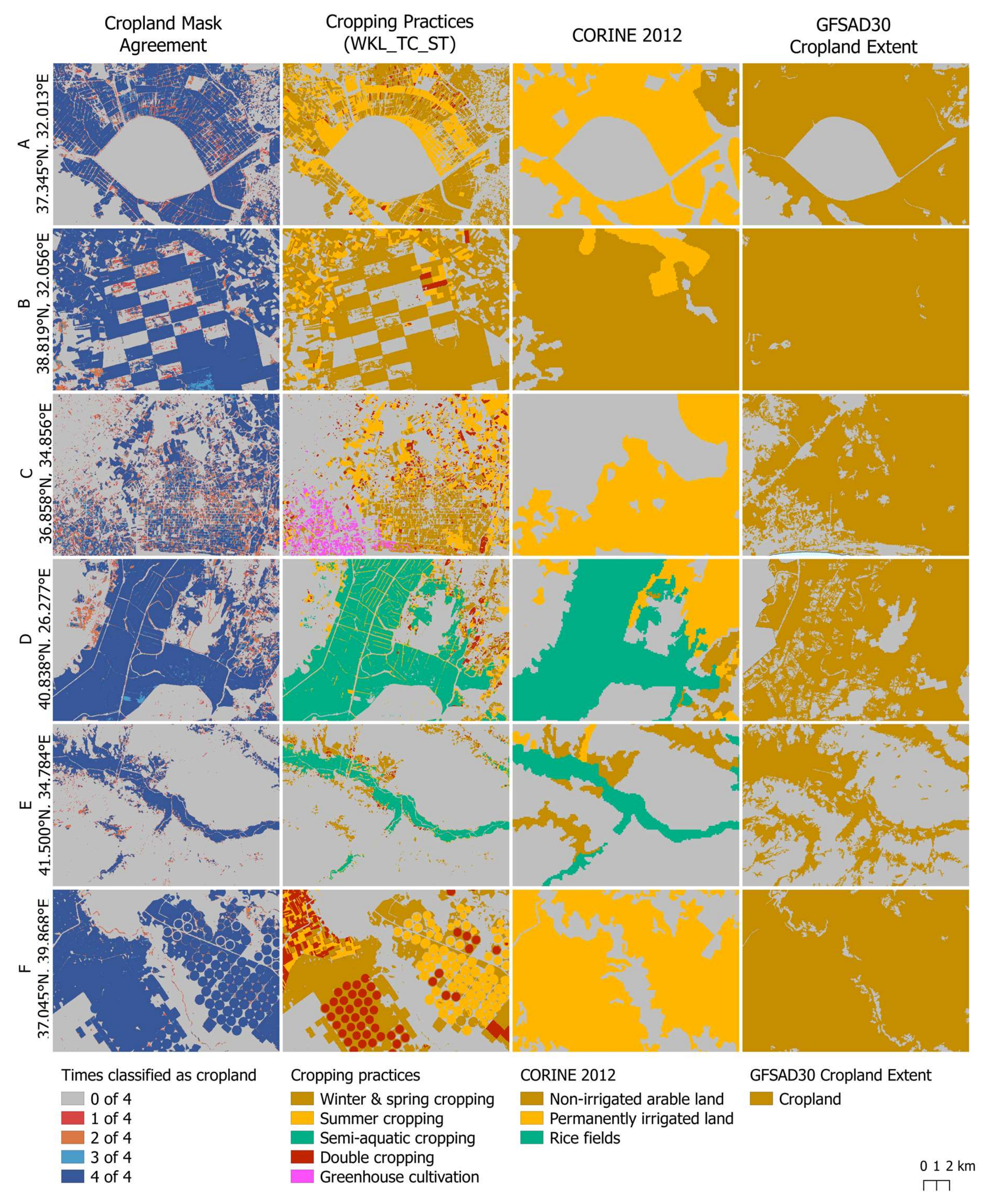
3.3. Evaluating Cropland Maps

Cropland area estimates of the maps with the highest accuracies ranged between 10.73 Mha and 11.72 Mha (±0.8 Mha; Table 4), thereby being substantially lower than reported statistics of cropland area extent, with a country total of 15.7 Mha [48].
We compared province-level (NUTS3) cropland proportions (%) from the binary cropland map WKL_TC_STATS, CORINE Land Cover 2012 [59] as well as the GFSAD30 cropland extent product with the baseline year 2015 [60] with reported statistics of the sown area for the year 2015 [48] (Figure 4). Linear regression revealed high correlation of the cropland extent estimates from WKL_TC_STATS (r2 = 0.85) and CORINE 2012 (r2 = 0.84), whereas the correlation with estimates from GFSAD30 was comparatively low (r2 = 0.64). Regression coefficients revealed the systematic underestimation of cropland area for our cropland mask (slope of regression: β = 1.1), although it was much lower than the overestimation in CORINE 2012 (β = 0.7) and GFSAD30 (β = 0.5). For a more detailed comparison of the province-level estimates, we investigated the accuracy (bias), precision (repeatability) and uncertainty (root mean squared error) of mapped versus reported cropland for all three products. We found lower accuracy compared to CORINE 2012 (i.e., a higher bias), but higher precision (i.e., higher consistency of the prediction) and similar uncertainty (Table 5). Our cropland area estimates had the highest precision of all products investigated here, and their uncertainty was similar to estimates obtained from CORINE 2012. However, the overestimation of cropland in GFSAD30 as well as CORINE 2012, as compared to the national statistics, might partly be related to the product class definitions, which include temporary fallow croplands.
We overlaid the binary cropland masks resulting from the four best classifications, finding agreement in 93.2% of the area, corresponding to 11.3% of cropland, and 81.9% of the other class. Disagreement across cropland masks (Figure 5, first column) occurred on parcel boundaries, within seasonally inundated wetlands and lakes, and in small-scale, fragmented or low-intensity cropping systems.
A comparison of the map products further demonstrated how these differences unfolded spatially and revealed some advantages of the presented cropping practice map (Figure 5). For instance, we captured parcels of temporary fallow croplands (e.g., Figure 5A–C). Furthermore, our mapping methods are pixel-based and thus not restricted to a minimum mapping unit, which allowed for capturing small parcels in fragmented landscapes (e.g., Figure 5C). Additionally, we found very high agreement between our semi-aquatic cropping class and CORINE’s rice field class (Figure 5D,E). The thematic detail of our maps allowed for identifying greenhouse cultivation (Figure 5C) or the distinction between winter, summer, and double cropping in intensively irrigated systems (Figure 5F).

3.4. Spatial Patterns of Cropping Practices

Error-adjusted class area estimates across the four models were consistent (Figure 6). According to the selected model (WKL_TC_STATS), spring and winter crops cover 71.3% (±2.3%), and summer crops 15.8% (±2.2%) of the total cropland area. Double cropping occurred on 8.5% (±1.6%), and semi-aquatic crops were cultivated on 4.0% (±1.9%) of the cropland area. Greenhouses accounted for only 0.32% (±0.2%) of the cropland area, corresponding to an estimated 36,752 ha, which is well in line with the 38,605 ha reported in official statistics [48].
We visually identified regional differences in cropping practices across Turkey (Figure 7). Semi-aquatic cropping, i.e., paddy rice cultivation, was prevalent in Sinop province in the Black Sea region (Figure 7A) and the Evros river valley alongside the Turkish-Greek border. Here, misclassifications of summer crops on the unflooded parcel-boundaries were apparent (Figure 7B). Distinct patterns of summer and double cropping occurred in the river valleys flowing into the Aegean Sea, most notably in the provinces of Aydın, Maniza, and İzmir (Figure 7C). Central parts of Anatolia contained large-scale cropping systems (Figure 7E). Agglomerations of greenhouses characterized the agricultural landscape along the Mediterranean coastline, e.g., East of Antalya (Figure 7D,F). We found intensive cultivation patterns in the Şanlıurfa and Mardin provinces of the South-East Anatolia Project irrigation scheme (Figure 7G). The cropping system in Eastern Anatolia showed heterogeneous parcel sizes and management systems, consisting of winter, summer, and double cropping (Figure 7H,I).
Province-level (NUTS-3) shares of annual cropland by province showed spatial hotspots of cropland in the Northwest, Central Anatolia, and South-Eastern Anatolia (Figure 8). Fractions of cropping practices in 2015 revealed the dominance of spring and winter cropping across Turkey. Fifty-three provinces were dominated (>60%) by winter and spring cropping. Summer cropping was the second most common cultivation strategy and distributed across almost all provinces, with spatial clusters along the Aegean Sea and the Eastern Mediterranean Sea. Double cropping occurred on less than 9% of croplands and clustered spatially in South-East Anatolia, e.g., Mardin (40%) and Şanlıurfa (21%), in the river valleys of the Aegean Sea region, e.g., İzmir (37%), and parts of the Black Sea region where cropland was limited. Semi-aquatic cropping was relevant in Edirne (21%) along the Greek border and Sinop (21%) in the Central Black Sea region. Greenhouse cultivation clustered along the Mediterranean coastline, especially Antalya (17%) and İçel (10%).

4. Discussion

The openly accessible Landsat archive provides unseen opportunities for informing land use intensity assessments over large areas. The presented study generated a set of good practice recommendations for mapping cropping practices over large areas, considerations for transferring the presented approaches into eras with different sensor constellations, uncertainties related to our approach, as well as insights concerning Turkey’s cropland management regimes.

4.1. Good Practice Recommendations

We highlight that the binning of dense image time series within pre-defined temporal windows is an efficient technique to produce widely consistent image features over space and time. Overall, the robustness, high classification accuracies and spatial consistency of our maps demonstrate the applicability of currently operational sensor constellations for mapping cropping practices across environmental and management gradients. We were able to identify some patterns when testing several temporal binning schemes and methods, which translate into a set of good practice recommendations.
First, retaining the seasonal information contained in the intra-annual time series is of the utmost importance for mapping cropping practices. Our tests revealed that annual binning into spectral-temporal metrics or time series statistics performed poorly, as the phenological information is lost (Figure 2). In line with a recently presented approach on crop type mapping [61], increasing the temporal resolution of the included features had a positive impact on classification accuracies. We thus suggest narrow, e.g., near-weekly binning wherever data availability, allows for satisfactory spatial coverage during cloud-prone seasons. Alternatively, quarterly binning provided a good trade-off between temporal detail and observation availability that allowed for producing robust results on national, up to continental scales [25].
Second, summer composites and spectral-temporal metrics produced satisfactory overall accuracies for Turkey. Thus, images from June to September essentially describe the spectral-temporal characteristics of our target classes. However, other seasonal windows might be more important when applying the approach in regions with different climate or management regimes. Similar to a study focusing on continental scale cropland mapping [25], classification accuracies increased when features from all quarters were included. Doing so presents an alternative to data-driven identification of the phenologically relevant season for accurate class discrimination or expert knowledge acquisition, as the first is challenging to implement and the latter is commonly not available in a spatially explicit manner across large areas.
Third, including auxiliary features describing geographic location and topography improved mapping accuracy. In line with other studies [62], we thus recommend the integration of such features in large area mapping as a common practice.
Our mapping efforts were relatively inexpensive. Two trained interpreters conducted the collection of training data and labeling of validation points in 320 work hours. Overall computation times were below two weeks for pre-processing, computation of all temporal features, and classification. However, we performed all computations using multi-core processing, which reduced processing times substantially. Storage space requirements were highest for pre-processed Landsat data (2.6 TB), composites and spectral-temporal metrics (0.8 TB), as well as Tasseled Cap time series and statistics (0.4 TB), but can be further reduced via image compression. In cases where processing and storage infrastructure is not available, processing can alternatively be performed using readily available ARD on cloud processing platforms [63]. The map product presented in this paper is available online (https://doi.pangaea.de/10.1594/PANGAEA.897547).

4.2. Temporal Transferability

The applicability of individual methods is dependent on the operational sensor constellation during the period of interest. For past decades, highly irregular inter-annual acquisition densities in the Landsat archive pose challenges for long-term mapping approaches [28]. Seasonally restricted spectral-temporal metrics are promising tools for mapping land use across large areas in past decades [31]. Average clear-sky observation density across Turkey between 1984 and 2017 is rarely below three observations during summer, suggesting that efforts targeting the mapping of cropping practices in Turkey over past decades are potentially worthwhile. However, these demand analyses of the quality of spectral-temporal features under scenarios of scarce and temporally disperse observations.
On the contrary, mapping cropping practices in the years past 2015 will benefit from novel sensor constellations with higher revisit frequency, which increases the probability of cloud-free acquisitions. Improvements of sensor integration [64,65] and automated image processing [66] now enable the combined use of intra-annual Landsat 8 and Sentinel 2A+B acquisitions for agricultural mapping applications [61]. Increased observation density will likely improve the mapping of cropland management interventions, such as harvests, or flooding of semi-aquatic crops. Recent advances also suggest the applicability of radar data to further supplement mapping efforts at high thematic detail [67], which can also be temporally aggregated for large area applications [68].

4.3. Uncertainties and Limitations

The products generated here meet common quality criteria regarding classification accuracy, and the high spatial consistency and thematic detail of these maps have the potential to satisfy the growing need for land use intensity datasets covering large areas [1,2]. However, remaining uncertainties relate to underestimated cropland extent and the omission of semi-aquatic cropping. We underestimated cropland extent by 25%, mostly due to confusion between spring crops and grasslands, as both classes represent herbaceous vegetation layers underlying precipitation-driven phenology and management interventions. Differences in cropland area estimates can be reduced by employing adaptive thresholds for classification probability, in order to match higher quality cropland area estimates, such as province-level statistics [18]. The omission of semi-aquatic cropping occurred due to the confusion with summer cropping, owing to strong phenological similarities. This insight supports the hypothesis that image availability during the flooding stage is crucial for accurate representation of semi-aquatic crops, such as paddy rice [69].
While our study aims at the characterization of annual croplands, spatially explicit information on grasslands and perennial croplands is essential for a better characterization of agricultural land use intensity [1]. In 2015, permanent pastures accounted for 14.6 Mha and perennial croplands for 3.3 Mha in Turkey [48], highlighting the need for detailed characterization of perennial crop systems to improve the understanding of the entire production system. However, the mapping of perennial croplands and grasslands poses various challenges from a remote sensing perspective [70,71,72]. These arise from heterogeneous class characteristics (crop type, grass species, phenology, planting density, irrigation, and mowing frequency) and the lack of datasets that allow for discriminating natural from managed grasslands, as well as cropped plantations from timber plantations.

4.4. Cropland Intensity and Water Resources in Turkey

Cropland management strongly determines agricultural water requirements [73,74]. We show that vast areas of annual croplands exist in semi-arid parts of Turkey, where total annual precipitation ranges between 200 mm and 600 mm, with near-zero precipitation during summer and particularly high evaporation rates [45]. While we show that spring and winter cropping, covering extensive areas of winter cereals with relatively low water requirements, dominate in Turkey [45,75], our results reveal that 28% of the national cropland area was cultivated during summer in 2015 (including summer, double, and semi-aquatic cropping). The recent expansion of irrigated agriculture, coupled with high irrigation water requirements led to a 48% increase in agricultural water requirements between 1992 and 2008 [76]. In the case of the South-East Anatolia Project, the expansion of irrigated cotton cultivation successfully boosted the regional economy [77], yet this occurred at the cost of drastic water consumption increases [49,78].
Current irrigation water use in Turkey is excessive and inefficient [44]. Generally, low water prices due to a lack of volumetric pricing schemes foster excessive water use [79]. Irrigation efficiencies in Turkey commonly do not exceed 50%, mostly due to the prevalence of surface irrigation, and high conveyance losses [80]. While the Turkish government envisions a 73% expansion of irrigated agriculture until 2030 [81], doing so without drastic institutional, agronomic, and engineering changes poses a threat to the national water resource base. Climate change further aggravates crop water deficits across Turkey [82], causing yield declines on rainfed and irrigated croplands [83,84]. The adoption of more efficient irrigation techniques offers water savings potential in the region [85], whereas saved water can be re-allocated and enable irrigation in other production systems [81,86]. Improving water use efficiency through reduced conveyance and evaporative losses is thus imperative to foster more sustainable production and should be of the utmost priority of planning authorities to prevent water scarcity and maintain environmental flow requirements in future intensification pathways [87].

5. Conclusions

We based our approach exclusively on openly available datasets (Landsat Collection 1 imagery) and algorithms (FORCE v1.1) that allow for streamlining pre-processing chains and producing analysis-ready datasets. We thereby demonstrated the benefits of openly accessible satellite image datasets and pre-processing frameworks for improving our understanding of agricultural land use intensity across large areas. This study provides a robust mapping framework to disentangle annual cropland management, using Turkey as a case study.
The fine spatial and temporal detail of the resulting maps allow for tracking cropping practices at 30 m spatial resolution and at annual intervals. Our maps can reveal areas of low cropland use intensity, such as rainfed cultivation on small parcels or fallow croplands, as opposed to intensity hotspots, such as double-cropped areas, flood-irrigated croplands, or areas with greenhouse cultivation. This is a substantial improvement compared to statistics at aggregated units, or other map products of reduced thematic detail, or coarser spatial or temporal resolution. The detail of our maps has the potential to inform stakeholder-related processes and assessments of land and water resource consumption over large areas.
We formulated good practice recommendations for binning Landsat time-series into temporal features for wall-to-wall characterization of cropping practices. We recommend binning into quarterly or finer temporal windows, wherever data availability is sufficient. We achieved the best classification results by using quarterly composites and spectral-temporal metrics, or gap-filled time series of Tasseled Cap components as input features. Auxiliary features on topography and geographic location improved classification accuracies throughout. Knowledge of regional phenological characteristics of the target classes is essential. However, we generally recommend the integration of features from multiple seasons, when difficulties in identifying key phenological windows prevail.
The generic temporal binning of all available clear sky observations into eight-day or quarterly time windows was a successful strategy in a Mediterranean setting but is likely applicable in climatic zones with a good data availability in the growing season. In this light, transferring our approach to other regions and eras requires investigating the effect of observation density on the consistency of temporal features, to determine minimum data requirements and subsequent trade-offs in mapping accuracies. The presented methods are potentially applicable across yearly time series to get insights into the inter-annual cropland management dynamics and to derive efficiency indicators such as irrigation ratios. Complementing the presented methods with techniques for detecting parcel sizes (e.g., References [17,88]) could enable the long-term evaluation of governmental land consolidation policies. Such information could ultimately improve our understanding of long-term developments of cropland management, and thus land and water resource demand at the regional to continental scale.

Author Contributions

Conceptualization, P.R., D.F., P.G., M.Ö. and P.H.; Formal analysis, P.R.; Methodology, P.R., D.F., A.R. and P.G.; Software, D.F., A.R. and P.G.; Supervision, P.H.; Validation, P.R. and S.E.; Writing—original draft, P.R.; Writing—review & editing, D.F., S.E., P.G., M.Ö. and P.H.

Funding

This research received no external funding.

Acknowledgments

This research contributes to the Landsat Science Team and the Global Land Programme. All authors acknowledge and appreciate the United States Geological Survey’s efforts in providing Landsat data. We thank the Turkish Statistical Institute for providing province-level statistics and the Global Food Security-Support Analysis Data at 30 m project for their efforts in global-scale cropland mapping. We acknowledge support by the German Research Foundation (DFG) and the Open Access Publication Fund of Humboldt-Universität zu Berlin.

Conflicts of Interest

The authors declare no conflict of interest.

Appendix A

Table A1. Confusion matrix for variable subset “ALL”. Cells populated with adjusted probabilities [54]. WC: winter cropping, SC: summer cropping, AC: semi-aquatic cropping, DC: double-cropping, GH: greenhouse cultivation.
Reference
WCSCACDCGH
ClassificationWC0.69530.00850.00420.01270.0000
SC0.01290.15280.02580.01100.0018
AC0.00000.00140.00500.00010.0000
DC0.00470.00710.00000.05440.0000
GH0.00000.00010.00000.00000.0021
Table A2. Confusion matrix for variable subset “QRT_CMP_STM”. Cells populated with adjusted probabilities [54]. WC: winter cropping, SC: summer cropping, AC: semi-aquatic cropping, DC: double-cropping, GH: greenhouse cultivation.
Reference
WCSCACDCGH
ClassificationWC0.69960.00850.00420.00850.0000
SC0.01660.16200.01840.00370.0037
AC0.00000.00140.00500.00010.0000
DC0.00830.01540.00000.04260.0000
GH0.00000.00010.00000.00000.0021
Table A3. Confusion matrix for variable subset “WKL_TC”. Cells populated with adjusted probabilities [54]. WC: winter cropping, SC: summer cropping, AC: semi-aquatic cropping, DC: double-cropping, GH: greenhouse cultivation.
Reference
WCSCACDCGH
ClassificationWC0.69530.00850.00420.01270.0000
SC0.01290.14730.03130.01290.0000
AC0.00000.00150.00490.00010.0000
DC0.00470.00830.00000.05200.0012
GH0.00000.00000.00000.00020.0020
Table A4. Confusion matrix for variable subset “WKL_TC_ST”. Cells populated with adjusted probabilities [54]. WC: winter cropping, SC: summer cropping, AC: semi-aquatic cropping, DC: double-cropping, GH: greenhouse cultivation.
Reference
WCSCACDCGH
ClassificationWC0.69530.00850.00420.01270.0000
SC0.01290.14360.03130.01660.0000
AC0.00000.00160.00480.00010.0000
DC0.00470.00470.00000.05560.0012
GH0.00000.00000.00000.00010.0020

Appendix B

Figure A1. Validation pixel protocol for class spring/winter crop.
Remotesensing 11 00232 g0a1
Figure A2. Validation pixel protocol for class summer crop.
Remotesensing 11 00232 g0a2
Figure A3. Validation pixel protocol for class semi-aquatic crop.
Remotesensing 11 00232 g0a3
Figure A4. Validation pixel protocol for class double cropping.
Remotesensing 11 00232 g0a4
Figure A5. Validation pixel protocol for class greenhouse.
Remotesensing 11 00232 g0a5

References

  1. Pongratz, J.; Dolman, H.; Don, A.; Erb, K.-H.; Fuchs, R.; Herold, M.; Jones, C.; Kuemmerle, T.; Luyssaert, S.; Meyfroidt, P.; et al. Models meet data: Challenges and opportunities in implementing land management in Earth system models. Glob. Chang. Biol. 2017, 1–18. [Google Scholar] [CrossRef] [PubMed]
  2. Kümmerle, T.; Erb, K.; Meyfroidt, P.; Müller, D.; Verburg, P.H.; Estel, S.; Haberl, H.; Hostert, P.; Jepsen, M.R.; Kastner, T.; et al. Challenges and opportunities in mapping land use intensity globally. Curr. Opin. Environ. Sustain. 2013, 5, 484–493. [Google Scholar] [CrossRef] [PubMed] [Green Version]
  3. Erb, K.-H.; Haberl, H.; Jepsen, M.R.; Kuemmerle, T.; Lindner, M.; Muller, D.; Verburg, P.H.; Reenberg, A. A conceptual framework for analysing and measuring land-use intensity. Curr. Opin. Environ. Sustain. 2013, 5, 464–470. [Google Scholar] [CrossRef] [PubMed] [Green Version]
  4. Bégué, A.; Arvor, D.; Bellon, B.; Betbeder, J.; de Abelleyra, D.; Ferraz, R.P.D.; Lebourgeois, V.; Lelong, C.; Simões, M.; Verón, S.R. Remote Sensing and Cropping Practices: A Review. Remote Sens. 2018, 10, 99. [Google Scholar] [CrossRef]
  5. Portmann, F.T.; Siebert, S.; Döll, P. MIRCA2000-Global monthly irrigated and rainfed crop areas around the year 2000: A new high-resolution data set for agricultural and hydrological modeling. Glob. Biogeochem. Cycles 2010, 24, 1–24. [Google Scholar] [CrossRef]
  6. Estel, S.; Kuemmerle, T.; Levers, C.; Baumann, M.; Hostert, P. Mapping cropland-use intensity across Europe using MODIS NDVI time series. Environ. Res. Lett. 2016, 11, 24015. [Google Scholar] [CrossRef]
  7. Jägermeyr, J.; Gerten, D.; Heinke, J.; Schaphoff, S.; Kummu, M.; Lucht, W. Water savings potentials of irrigation systems: global simulation of processes and linkages. Hydrol. Earth Syst. Sci. 2015, 19, 3073–3091. [Google Scholar] [CrossRef]
  8. Whitcraft, A.K.; Vermote, E.F.; Becker-Reshef, I.; Justice, C.O. Cloud cover throughout the agricultural growing season: Impacts on passive optical earth observations. Remote Sens. Environ. 2015, 438–447. [Google Scholar] [CrossRef]
  9. Jain, M.; Mondal, P.; DeFries, R.S.; Small, C.; Galford, G.L. Mapping cropping intensity of smallholder farms: A comparison of methods using multiple sensors. Remote Sens. Environ. 2013, 134, 210–223. [Google Scholar] [CrossRef]
  10. Biradar, C.M.; Xiao, X. Quantifying the area and spatial distribution of double- and triple-cropping croplands in India with multi-temporal MODIS imagery in 2005. Int. J. Remote Sens. 2011, 32, 367–386. [Google Scholar] [CrossRef]
  11. Salmon, J.M.; Friedl, M.A.; Frolking, S.; Wisser, D.; Douglas, E.M. Global rain-fed, irrigated, and paddy croplands: A new high resolution map derived from remote sensing, crop inventories and climate data. Int. J. Appl. Earth Observ. Geoinf. 2015, 38, 321–334. [Google Scholar] [CrossRef]
  12. Thenkabail, P.S.; Dheeravath, V.; Biradar, C.M.; Gangalakunta, O.R.P.; Noojipady, P.; Gurappa, C.; Velpuri, M.; Gumma, M.; Li, Y. Irrigated Area Maps and Statistics of India Using Remote Sensing and National Statistics. Remote Sens. 2009, 1, 50–67. [Google Scholar] [CrossRef] [Green Version]
  13. Velpuri, N.M.; Thenkabail, P.S.; Gumma, M.K.; Biradar, C.; Dheeravath, V.; Noojipady, P.; Yuanjie, L. Influence of Resolution in Irrigated Area Mapping and Area Estimation. Photogramm. Eng. Remote Sens. 2009, 75, 1383–1395. [Google Scholar] [CrossRef]
  14. Deines, J.M.; Kendall, A.D.; Hyndman, D.W. Annual Irrigation Dynamics in the U.S. Northern High Plains Derived from Landsat Satellite Data. Geophys. Res. Lett. 2017, 44, 9350–9360. [Google Scholar] [CrossRef]
  15. Ferrant, S.; Selles, A.; Le Page, M.; Herrault, P.-A.; Pelletier, C.; Al-Bitar, A.; Mermoz, S.; Gascoin, S.; Bouvet, A.; Saqalli, M.; et al. Detection of Irrigated Crops from Sentinel-1 and Sentinel-2 Data to Estimate Seasonal Groundwater Use in South India. Remote Sens. 2017, 9, 1119. [Google Scholar] [CrossRef]
  16. Chen, Y.; Lu, D.; Luo, L.; Pokhrel, Y.; Deb, K.; Huang, J.; Ran, Y. Detecting irrigation extent, frequency, and timing in a heterogeneous arid agricultural region using MODIS time series, Landsat imagery, and ancillary data. Remote Sens. Environ. 2018, 197–211. [Google Scholar] [CrossRef]
  17. Graesser, J.; Ramankutty, N. Detection of cropland field parcels from Landsat imagery. Remote Sens. Environ. 2017, 201, 165–180. [Google Scholar] [CrossRef]
  18. Song, X.-P.; Potapov, P.V.; Krylov, A.; King, L.; Di Bella, C.M.; Hudson, A.; Khan, A.; Adusei, B.; Stehman, S.V.; Hansen, M.C. National-scale soybean mapping and area estimation in the United States using medium resolution satellite imagery and field survey. Remote Sens. Environ. 2017, 190, 383–395. [Google Scholar] [CrossRef]
  19. Wulder, M.A.; White, J.C.; Goward, S.N.; Masek, J.G.; Irons, J.R.; Herold, M.; Cohen, W.B.; Loveland, T.R.; Woodcock, C.E. Landsat continuity: Issues and opportunities for land cover monitoring. Remote Sens. Environ. 2008, 112, 955–969. [Google Scholar] [CrossRef]
  20. Arvidson, T.; Gasch, J.; Goward, S.N. Landsat 7’s long-term acquisition plan—An innovative approach to building a global imagery archive. Remote Sens. Environ. 2001, 78, 13–26. [Google Scholar] [CrossRef]
  21. Kovalskyy, V.; Roy, D.P. The global availability of Landsat 5 TM and Landsat 7 ETM+ land surface observations and implications for global 30m Landsat data product generation. Remote Sens. Environ. 2013, 130, 280–293. [Google Scholar] [CrossRef] [Green Version]
  22. Kovalskyy, V.; Roy, D. A One Year Landsat 8 Conterminous United States Study of Cirrus and Non-Cirrus Clouds. Remote Sens. 2015, 7, 564–578. [Google Scholar] [CrossRef] [Green Version]
  23. Gómez, C.; White, J.C.; Wulder, M.A. Optical remotely sensed time series data for land cover classification: A review. ISPRS J. Photogramm. Remote Sens. 2016, 116, 55–72. [Google Scholar] [CrossRef] [Green Version]
  24. Waldner, F.; Canto, G.S.; Defourny, P. Automated annual cropland mapping using knowledge-based temporal features. ISPRS J. Photogramm. Remote Sens. 2015, 110, 1–13. [Google Scholar] [CrossRef]
  25. Phalke, A.R.; Özdoğan, M. Large area cropland extent mapping with Landsat data and a generalized classifier. Remote Sens. Environ. 2018, 219, 180–195. [Google Scholar] [CrossRef]
  26. Griffiths, P.; van der Linden, S.; Kuemmerle, T.; Hostert, P. A Pixel-Based Landsat Compositing Algorithm for Large Area Land Cover Mapping. IEEE J. Sel. Top. Appl. Earth Observ. Remote Sens. 2013, 6, 2088–2101. [Google Scholar] [CrossRef]
  27. Frantz, D.; Röder, A.; Stellmes, M.; Hill, J. Phenology-adaptive pixel-based compositing using optical earth observation imagery. Remote Sens. Environ. 2017, 190, 331–347. [Google Scholar] [CrossRef]
  28. Griffiths, P.; Jakimow, B.; Hostert, P. Reconstructing long term annual deforestation dynamics in Pará and Mato Grosso using the Landsat archive. Remote Sens. Environ. 2018, 216, 497–513. [Google Scholar] [CrossRef]
  29. Pasquarella, V.J.; Holden, C.E.; Woodcock, C.E. Improved mapping of forest type using spectral-temporal Landsat features. Remote Sens. Environ. 2018, 210, 193–207. [Google Scholar] [CrossRef]
  30. Müller, H.; Rufin, P.; Griffiths, P.; Siqueira, A.J.B.; Hostert, P. Mining dense Landsat time series for separating cropland and pasture in a heterogeneous Brazilian savanna landscape. Remote Sens. Environ. 2015, 156, 490–499. [Google Scholar] [CrossRef] [Green Version]
  31. Schmidt, M.; Pringle, M.; Devadas, R.; Denham, R.; Tindall, D. A Framework for Large-Area Mapping of Past and Present Cropping Activity Using Seasonal Landsat Images and Time Series Metrics. Remote Sens. 2016, 8, 312. [Google Scholar] [CrossRef]
  32. Gao, F.; Masek, J.; Schwaller, M.; Hall, F. On the blending of the Landsat and MODIS surface reflectance: predicting daily Landsat surface reflectance. IEEE Trans. Geosci. Remote Sens. 2006, 44, 2207–2218. [Google Scholar] [CrossRef]
  33. Gao, F.; Anderson, M.C.; Zhang, X.; Yang, Z.; Alfieri, J.G.; Kustas, W.P.; Mueller, R.; Johnson, D.M.; Prueger, J.H. Toward mapping crop progress at field scales through fusion of Landsat and MODIS imagery. Remote Sens. Environ. 2017, 188, 9–25. [Google Scholar] [CrossRef]
  34. Schwieder, M.; Leitão, P.J.; da Cunha Bustamante, M.M.; Ferreira, L.G.; Rabe, A.; Hostert, P. Mapping Brazilian savanna vegetation gradients with Landsat time series. Int. J. Appl. Earth Observ. Geoinf. 2016, 52, 361–370. [Google Scholar] [CrossRef]
  35. Waldner, F.; Hansen, M.C.; Potapov, P.V.; Löw, F.; Newby, T.; Ferreira, S.; Defourny, P. National-scale cropland mapping based on spectral-temporal features and outdated land cover information. PLoS ONE 2017, 12, e0181911. [Google Scholar] [CrossRef] [PubMed]
  36. Ambika, A.K.; Wardlow, B.; Mishra, V. Remotely sensed high resolution irrigated area mapping in India for 2000 to 2015. Sci. Data 2016, 3, 160118. [Google Scholar] [CrossRef] [Green Version]
  37. Son, N.-T.; Chen, C.-F.; Chen, C.-R.; Duc, H.-N.; Chang, L.-Y. A Phenology-Based Classification of Time-Series MODIS Data for Rice Crop Monitoring in Mekong Delta, Vietnam. Remote Sens. 2014, 6, 135–156. [Google Scholar] [CrossRef]
  38. Özdoğan, M.; Yang, Y.; Allez, G.; Cervantes, C. Remote Sensing of Irrigated Agriculture: Opportunities and Challenges. Remote Sens. 2010, 2, 2274–2304. [Google Scholar] [CrossRef] [Green Version]
  39. Jönsson, P.; Eklundh, L. TIMESAT—A program for analyzing time-series of satellite sensor data. Comput. Geosci. 2004, 30, 833–845. [Google Scholar] [CrossRef]
  40. Griffiths, P.; Kuemmerle, T.; Baumann, M.; Radeloff, V.C.; Abrudan, I.V.; Lieskovsky, J.; Munteanu, C.; Ostapowicz, K.; Hostert, P. Forest disturbances, forest recovery, and changes in forest types across the Carpathian ecoregion from 1985 to 2010 based on Landsat image composites. Remote Sens. Environ. 2014, 151, 72–88. [Google Scholar] [CrossRef]
  41. Melaas, E.K.; Friedl, M.A.; Zhu, Z. Detecting interannual variation in deciduous broadleaf forest phenology using Landsat TM/ETM+ data. Remote Sens. Environ. 2013, 132, 176–185. [Google Scholar] [CrossRef]
  42. Yaslioglu, E.; Akkaya Aslan, S.T.; Kirmikil, M.; Gundogdu, K.S.; Arici, I. Changes in Farm Management and Agricultural Activities and Their Effect on Farmers’ Satisfaction from Land Consolidation: The Case of Bursa–Karacabey, Turkey. Eur. Plan. Stud. 2009, 17, 327–340. [Google Scholar] [CrossRef]
  43. Kibaroğlu, A.; Sümer, V.; Scheumann, W. Fundamental Shifts in Turkey’s Water Policy. Mediterranee 2012, 27–34. [Google Scholar] [CrossRef]
  44. Kibaroğlu, A.; Kramer, A.; Scheumann, W. Turkey’s Water Policy. National Frameworks and International Cooperation; Springer: Berlin/Heidelberg, Germany; New York, NY, USA, 2011. [Google Scholar]
  45. FAO. Irrigation in the Middle East Region. Country Profile: Turkey; AQUASTAT Survey-2008 No. 34; FAO: Rome, Italy, 2009. [Google Scholar]
  46. Dwyer, J.; Roy, D.; Sauer, B.; Jenkerson, C.; Zhang, H.; Lymburner, L. Analysis Ready Data: Enabling Analysis of the Landsat Archive. Remote Sens. 2018, 10, 1–19. [Google Scholar] [CrossRef]
  47. Frantz, D. Generation of Higher Level Earth Observation Satellite Products for Regional Environmental Monitoring. Ph.D. Thesis, Universität Trier, Trier, Germany, 2017. [Google Scholar]
  48. TSI. Crop Production Statistics. Agricultural Land. 2015. Available online: http://www.turkstat.gov.tr/ (accessed on 1 April 2018).
  49. Özdoğan, M.; Woodcock, C.E.; Salvucci, G.D.; Demir, H. Changes in Summer Irrigated Crop Area and Water Use in Southeastern Turkey from 1993 to 2002: Implications for Current and Future Water Resources. Water Resour. Manag. 2006, 20, 467–488. [Google Scholar] [CrossRef] [Green Version]
  50. Radeloff, V.; Yin, H.; Tan, B.; Frantz, D.; Buchner, J. Topographic Correction of Landsat imagery in the Caucasus Mountains; Landsat Science Team Meeting; USGS: Boulder, Colorado, 2018. Available online: https://landsat.usgs.gov/landsat-science-team-meeting-august-8-10-2018 (accessed on 21 January 2019).
  51. Tan, B.; Masek, J.G.; Wolfe, R.; Gao, F.; Huang, C.; Vermote, E.F.; Sexton, J.O.; Ederer, G. Improved forest change detection with terrain illumination corrected Landsat images. Remote Sens. Environ. 2013, 136, 469–483. [Google Scholar] [CrossRef]
  52. Frantz, D.; Roder, A.; Stellmes, M.; Hill, J. An Operational Radiometric Landsat Preprocessing Framework for Large-Area Time Series Applications. IEEE Trans. Geosci. Remote Sens. 2016, 54, 3928–3943. [Google Scholar] [CrossRef]
  53. USGS. SRTM 1 Arc-Second Global. Available online: https://lta.cr.usgs.gov/SRTM1Ar (accessed on 1 April 2016).
  54. Olofsson, P.; Foody, G.M.; Herold, M.; Stehman, S.V.; Woodcock, C.E.; Wulder, M.A. Good practices for estimating area and assessing accuracy of land change. Remote Sens. Environ. 2014, 148, 42–57. [Google Scholar] [CrossRef] [Green Version]
  55. Crist, E.P.; Cicone, R.C. A Physically Based Transformation of Thematic Mapper Data—The TM Tasseled Cap. IEEE Trans. Geosci. Remote Sens. 1984, 3, 256–263. [Google Scholar] [CrossRef]
  56. Crist, E.P. A TM tasseled cap equivalent transformation for reflectance factor data. Remote Sens. Environ. 1985, 301–306. [Google Scholar] [CrossRef]
  57. Cochran, W.G. Sampling Techniques, 3rd ed.; Wiley: Hoboken, NJ, USA, 1977. [Google Scholar]
  58. Breiman, L. Random Forests. Mach. Learn. 2001, 45, 5–32. [Google Scholar] [CrossRef] [Green Version]
  59. European Commission. Corine Land Cover (CLC) 2012 Version 18.5.1. 2017. Available online: https://land.copernicus.eu/pan-european/corine-land-cover/clc-2012 (accessed on 8 December 2017).
  60. Phalke, A.; Özdoğan, M.; Thenkabail, P.; Congalton, R.; Yadav, K.; Massey, R.; Teluguntla, P.; Poehnelt, J.; Smith, C. Global Food Security-Support Analysis Data (GFSAD) Cropland Extent 2015 Europe, Central Asia, Russia; Middle East 30 m V001: Sioux Falls, SD, USA, 2017. [Google Scholar]
  61. Griffiths, P.; Nendel, C.; Hostert, P. Intra-annual reflectance composites from Sentinel-2 and Landsat for national-scale crop and land cover mapping. Remote Sens. Environ. 2019, 220, 135–151. [Google Scholar] [CrossRef]
  62. Pflugmacher, D.; Rabe, A.; Peters, M.; Hostert, P. Mapping pan-European land cover using Landsat spectral-temporal metrics and the European LUCAS survey. Remote Sens. Environ. 2019, 221, 583–595. [Google Scholar] [CrossRef]
  63. Gorelick, N.; Hancher, M.; Dixon, M.; Ilyushchenko, S.; Thau, D.; Moore, R. Google Earth Engine: Planetary-scale geospatial analysis for everyone. Remote Sens. Environ. 2017, 202, 18–27. [Google Scholar] [CrossRef]
  64. Zhang, H.K.; Roy, D.P.; Yan, L.; Li, Z.; Huang, H.; Vermote, E.; Skakun, S.; Roger, J.-C. Characterization of Sentinel-2A and Landsat-8 top of atmosphere, surface, and nadir BRDF adjusted reflectance and NDVI differences. Remote Sens. Environ. 2018, 215, 482–494. [Google Scholar] [CrossRef]
  65. Claverie, M.; Ju, J.; Masek, J.G.; Dungan, J.L.; Vermote, E.F.; Roger, J.C.; Skakun, S.V.; Justice, C.O. The Harmonized Landsat and Sentinel-2 surface reflectance data set. Remote Sens. Environ. 2018. [Google Scholar] [CrossRef]
  66. Frantz, D.; Haß, E.; Uhl, A.; Stoffels, J.; Hill, J. Improvement of the Fmask algorithm for Sentinel-2 images: Separating clouds from bright surfaces based on parallax effects. Remote Sens. Environ. 2018, 471–481. [Google Scholar] [CrossRef]
  67. Mansaray, L.; Huang, W.; Zhang, D.; Huang, J.; Li, J. Mapping Rice Fields in Urban Shanghai, Southeast China, Using Sentinel-1A and Landsat 8 Datasets. Remote Sens. 2017, 9, 257. [Google Scholar] [CrossRef]
  68. Baumann, M.; Levers, C.; Macchi, L.; Bluhm, H.; Waske, B.; Gasparri, N.I.; Kuemmerle, T. Mapping continuous fields of tree and shrub cover across the Gran Chaco using Landsat 8 and Sentinel-1 data. Remote Sens. Environ. 2018, 216, 201–211. [Google Scholar] [CrossRef]
  69. Kontgis, C.; Schneider, A.; Özdoğan, M. Mapping rice paddy extent and intensification in the Vietnamese Mekong River Delta with dense time stacks of Landsat data. Remote Sens. Environ. 2015, 169, 255–269. [Google Scholar] [CrossRef]
  70. Vieira, M.A.; Formaggio, A.R.; Rennó, C.D.; Atzberger, C.; Aguiar, D.A.; Mello, M.P. Object Based Image Analysis and Data Mining applied to a remotely sensed Landsat time-series to map sugarcane over large areas. Remote Sens. Environ. 2012, 123, 553–562. [Google Scholar] [CrossRef]
  71. Senf, C.; Pflugmacher, D.; van der Linden, S.; Hostert, P. Mapping Rubber Plantations and Natural Forests in Xishuangbanna (Southwest China) Using Multi-Spectral Phenological Metrics from MODIS Time Series. Remote Sens. 2013, 5, 2795–2812. [Google Scholar] [CrossRef] [Green Version]
  72. Ali, I.; Cawkwell, F.; Dwyer, E.; Barrett, B.; Green, S. Satellite remote sensing of grasslands: from observation to management. JPECOL 2016, 9, 649–671. [Google Scholar] [CrossRef] [Green Version]
  73. Döll, P.; Siebert, S. Global modeling of irrigation water requirements. Water Resour. Res. 2002, 38, 1–10. [Google Scholar] [CrossRef]
  74. Rockström, J.; Karlberg, L.; Wani, S.P.; Barron, J.; Hatibu, N.; Oweis, T.; Bruggeman, A.; Farahani, J.; Qiang, Z. Managing water in rainfed agriculture—The need for a paradigm shift. Agric. Water Manag. 2010, 97, 543–550. [Google Scholar] [CrossRef]
  75. Lopes, M.S.; Royo, C.; Alvaro, F.; Sanchez-Garcia, M.; Ozer, E.; Ozdemir, F.; Karaman, M.; Roustaii, M.; Jalal-Kamali, M.R.; Pequeno, D. Optimizing Winter Wheat Resilience to Climate Change in Rain Fed Crop Systems of Turkey and Iran. Front. Plant Sci. 2018, 9, 563. [Google Scholar] [CrossRef] [PubMed]
  76. FAO. AQUASTAT Database. Available online: http://www.fao.org/nr/water/aquastat/data/ (accessed on 15 May 2015).
  77. Altinbilek, D.; Tortajada, C. The Atatürk Dam in the Context of the Southeastern Anatolia (GAP) Project. In Impacts of Large Dams: A Global Assessment; Tortajada, C., Altinbilek, D., Biswas, A.K., Eds.; Springer: Berlin/Heidelberg, Germany, 2012; pp. 171–199. [Google Scholar]
  78. Yesilnacar, M.I.; Uyanik, S. Investigation of water quality of the world’s largest irrigation tunnel system, the Sanliurfa Tunnels in Turkey. Fresenius Environ. Bull. 2005, 14, 300–306. [Google Scholar]
  79. Cakmak, E.H. Agricultural Water Pricing in Turkey. Economic Co-Operation and Development; OECD: Paris, France, 2010. [Google Scholar]
  80. Koç, C. Sustainability of Irrigation Schemes Transferred in Turkey. Irrig. Drain. 2017, 7, 231. [Google Scholar] [CrossRef]
  81. Büyükcangaz, H.; Demirtas, C.; Yazgan, S.; Korukcu, A. Efficient water use in agriculture in Turkey: The need for pressurized irrigation systems. Water Int. 2007, 32, 776–785. [Google Scholar] [CrossRef]
  82. EEA. Crop Water Demand: How Is Climate Change Affecting the Water Requirement of Agricultural Crops across Europe? Available online: https://www.eea.europa.eu/data-and-maps/indicators/water-requirement-2/assessment (accessed on 12 December 2018).
  83. Saadi, S.; Todorovic, M.; Tanasijevic, L.; Pereira, L.S.; Pizzigalli, C.; Lionello, P. Climate change and Mediterranean agriculture: Impacts on winter wheat and tomato crop evapotranspiration, irrigation requirements and yield. Agric. Water Manag. 2015, 147, 103–115. [Google Scholar] [CrossRef]
  84. Yano, T.; Aydin, M.; Haraguchi, T. Impact of Climate Change on Irrigation Demand and Crop Growth in a Mediterranean Environment of Turkey. Sensors 2007, 7, 2297–2315. [Google Scholar] [CrossRef] [PubMed] [Green Version]
  85. Ertek, A.; Yilmaz, H. The agricultural perspective on water conservation in Turkey. Agric. Water Manag. 2014, 143, 151–158. [Google Scholar] [CrossRef]
  86. Jägermeyr, J.; Gerten, D.; Schaphoff, S.; Heinke, J.; Lucht, W.; Rockström, J. Integrated crop water management might sustainably halve the global food gap. Environ. Res. Lett. 2016, 11, 25002. [Google Scholar] [CrossRef] [Green Version]
  87. Jägermeyr, J.; Pastor, A.; Biemans, H.; Gerten, D. Reconciling irrigated food production with environmental flows for Sustainable Development Goals implementation. Nat. Commun. 2017, 8, 15900. [Google Scholar] [CrossRef] [PubMed] [Green Version]
  88. Yan, L.; Roy, D.P. Conterminous United States crop field size quantification from multi-temporal Landsat data. Remote Sens. Environ. 2016, 172, 67–86. [Google Scholar] [CrossRef] [Green Version]
Figure 1. Study area and clear-sky observation count for 2015. Overlay represents the 63 Landsat WRS-2 scenes covering Turkey.
Remotesensing 11 00232 g001
Figure 2. Area adjusted overall accuracies for binary annual cropland classification (black) and cropping practice classification (grey), for 22 feature subsets. Error bars indicate 95% confidence intervals, vertical dashed line marks 90% accuracy.
Remotesensing 11 00232 g002
Figure 3. Area-adjusted producer’s (black) and user’s accuracies (grey) for the selected models. Error bars indicate 95% confidence intervals. Vertical dashed lines mark 90% accuracy.
Remotesensing 11 00232 g003
Figure 4. Comparison of province level fraction of cropland derived from maps and statistics from Turkish Statistical Institute at NUTS3-level (provinces; n = 81). Cropland extent mapped from WKL_TC_STATS (left), CORINE 2012 (center), and GFSAD30 (right). Grey line shows 1:1 line, the red dashed line represents linear regression line of the mapped area against statistics.
Remotesensing 11 00232 g004
Figure 5. Image subsets (rows A to F) of cropland mask overlay (first column), cropping practice product (second column), CORINE 2012 (third column) and GFSAD30 product (fourth column). Center coordinates of each subset indicated to the left.
Remotesensing 11 00232 g005
Figure 6. Error-adjusted area estimates of cropping practice classes (from left to right: winter/spring cropping, summer cropping, double cropping, semi-aquatic cropping, greenhouse cultivation) across the four best classification models (see Table 2 for abbreviations). Error bars indicate 95% confidence intervals.
Remotesensing 11 00232 g006
Figure 7. National-scale cropping practice map for the year 2015 (upper section), based on eight-day time-series of Tasseled Cap Brightness, Greenness, and Wetness including four annual statistics (WKL_TC_STATS). Black rectangles indicate location of subsets A to I (lower section).
Remotesensing 11 00232 g007
Figure 8. Province-level (NUTS-03) share of annual cropland on total province area (top left) and shares of cropping practices in percent of all cropland (remainder).
Remotesensing 11 00232 g008
Table 1. Description of the class catalog.
CategoryCropland ClassesDescription
Annual croplandWinter and spring croppingStart of the green-up possible in 2014, season peak around April/May 2015, followed by harvest.
Summer croppingSummer crops, start of the season in 2015, peak of the season between June and August, harvest in 2015.
Semi-aquatic croppingPhenology similar to summer crops, with visible flooding of parcels before green-up.
Double croppingTwo growing cycles and harvests within 2015, comprising winter and spring as well as summer cropping.
Greenhouse cultivationSpectrally bright due to foil cover with transmitted vegetation signal, which shows clear seasonality. Single or multiple seasons are possible.
Other-Includes deciduous and evergreen forests and shrublands with a closed canopy, open woodland and shrubland canopy with exposed soil background, plantations and perennial crops, natural, semi-natural and managed grasslands, marginal lands, such as bare soils without distinct phenology as well as built-up areas, wetlands, and surface water.
Table 2. Feature subsets and abbreviations, as well as total number of features, and number of features including the four auxiliary variables (latitude, longitude, elevation, and hillslope).
SchemeFeature SetModel AbbreviationN Feat.
AnnualAll featuresALL505
Annual spectral-temporal metricsANNUAL_STM70
Quarterly composites & quarterly spectral-temporal metricsQRT_STM_CMP292
Quarterly spectral-temporal metricsQRT_STM268
Quarterly compositesQRT_CMP28
TC statisticsTC_STATS16
Bi-quarterlyQ1 + Q2 composites & spectral-temporal metricsQ1Q2_STM_CMP148
Q1 + Q3 composites & spectral-temporal metricsQ1Q3_STM_CMP148
Q1 + Q4 composites & spectral-temporal metricsQ1Q4_STM_CMP148
Q2 + Q3 composites & spectral-temporal metricsQ2Q3_STM_CMP148
Q2 + Q4 composites & spectral-temporal metricsQ2Q4_STM_CMP148
Q3 + Q4 composites & spectral-temporal metricsQ3Q4_STM_CMP148
QuarterlyQ1 composites & spectral-temporal metricsQ1_STM_CMP76
Q2 composites & spectral-temporal metricsQ2_STM_CMP76
Q3 composites & spectral-temporal metricsQ3_STM_CMP76
Q4 composites & spectral-temporal metricsQ4_STM_CMP76
Quarterly & annualQ1 composites & spectral-temporal metrics & annual spectral-temporal metricsQ1_STM_CMP_ANN_STM142
Q2 composites & spectral-temporal metrics & annual spectral-temporal metricsQ2_STM_CMP_ANN_STM142
Q3 composites & spectral-temporal metrics & annual spectral-temporal metricsQ3_STM_CMP_ANN_STM142
Q4 composites & spectral-temporal metrics & annual spectral-temporal metricsQ4_STM_CMP_ANN_STM142
Weekly8-day TC time series & annual TC statisticsWKL_TC_STATS154
8-day TC time seriesWKL_TC139
Table 3. Landsat clear sky observation statistics for Turkey, 2015.
QuarterMean CSO CountMaximum CSO CountNo DataArea with Three or More CSOsArea with Five or More CSOsArea with Ten or More CSOs
1 (Jan–Mar)3.14169.17%57.92%23.78%0.67%
2 (Apr–Jun)6.37221.09%91.66%70.13%15.58%
3 (Jul–Sep)10.70240.07%99.48%96.74%55.74%
4 (Oct–Nov)6.61221.12%91.59%73.91%18.51%
Table 4. Error-adjusted cropland area estimates for Turkey in 2015. See Table 2 for abbreviations of model names.
Feature SubsetEstimated Cropland (Mha)95% Confidence Interval (Mha)
ALL11.41±0.81
QRT_CMP_STM10.73±0.83
WKL_TC11.36±0.77
WKL_TC_STATS11.72±0.79
Table 5. Model performance and summary statistics of linear regressions with NUTS3-level (n = 81), using cropland extent statistics as a dependent, and mapped cropland extent from WKL_TC_STATS, CORINE 2012, and GFSAD30 products as the independent variable. Accuracy, precision, and uncertainty in thousand hectares.
ModelAccuracyPrecisionUncertaintyr2
WKL_TC_STATS5.454.707.200.85
CORINE 2012−2.606.547.040.84
GFSAD30−21.8412.3825.110.64

