


1. INTRODUCTION
Assessing the impacts of climate change in glacierized regions requires accurate quantification of glacier mass balances in recent decades (IPCC, 2013). Although glaciological mass balance observations have been available in a few locations for five to six decades, in situ long-term observations in some regions remain scarce (Zemp and others, Reference Zemp2015). For instance, there is a lack of glacier mass balance records in the Andes, an area where only few glaciers have long-term monitoring series dating back to the beginning of the 1990s (Rabatel and others, Reference Rabatel2013). The availability of aerial surveys of this region since the 1950s makes the geodetic approach an adequate method to reconstruct a glacier mass balance. The geodetic method estimates changes in the mass of the glacier by the difference in the elevation of the glacier surface over a period of time (dh/dt) (Cogley and others, Reference Cogley2011), while assuming the average density associated with the volumetric change (Bader, Reference Bader1960; Paterson and Cuffey, Reference Paterson and Cuffey2010). The geodetic mass balance is formally reported in meter water equivalent per year (m w.e. a−1) (Cogley and others, Reference Cogley2011). This method requires accurate measurements of elevation at sufficiently long-time intervals to allow the signal of elevation change to be statistically significant, in view of measurement errors and the natural variability of the glacier mass balance (Bamber and Rivera, Reference Bamber and Rivera2007).
Nowadays, very high-resolution stereo images from aerial photos (e.g. DMC or ADS40 systems) or satellite data (e.g. Pléiades, SPOT, Worldview) and progress in modern photogrammetry/structure-from-motion techniques, allow accurate digital elevation models (DEMs) to be produced. Past changes in glacier surface elevation can be documented using historical aerial photographs acquired from the middle of the 20th century on (Rabatel and others, Reference Rabatel, Machaca, Francou and Jomelli2006; Soruco and others, Reference Soruco2009; Basantes-Serrano and others, Reference Basantes-Serrano2016). Progress in computational power and software capabilities since the 1990s has facilitated automation of this task due to the emergence and improvements of automatic pattern recognition techniques, often referred to as ‘stereo-matching algorithms’ (i.e. Baillard and others, Reference Baillard, Dissard, Jamet and Maître1998; Gruen and Akca, Reference Gruen and Akca2005; Hirschmuller, Reference Hirschmuller2005; Shean and others, Reference Shean2016). However, automatic processes may fail to produce reliable results over snow-covered surfaces with low contrast, and in the shadowed areas commonly found in mountainous terrain (Pellikka and Rees, Reference Pellikka and Rees2010; Berthier and others, Reference Berthier2014; Noh and Howat, Reference Noh and Howat2015; Magnússon and others, Reference Magnússon, Muñoz-Cobo Belart, Pálsson, Ágústsson and Crochet2016). Snow cover or shadows in stereo models result in a lack of stereoscopic measurements (Maurer and others, Reference Maurer, Rupper and Schaefer2016). In turn, the interpolation of such gaps can lead to false representations of the terrain (e.g. a knoll, plateau or depression) and introduce errors in the quantification of the glacier-wide mass balance (Thibert and others, Reference Thibert, Blanc, Vincent and Eckert2008). In order to address this issue, manual photogrammetric data collection sometimes remains a necessity, and is usually performed using two methods:
(i) A 3D point cloud, hereafter called ‘sampling points’, can be measured manually by photogrammetric restitution following a discrete procedure based on a regular or irregular grid (Basantes-Serrano and others, Reference Basantes-Serrano2016). The restituted points can then be interpolated to produce a DEM. This approach requires expert photogrammetric interpretation to overcome the pitfalls of automatic stereo-matching in challenging terrain and has been applied successfully on several glaciers (Thibert and others, Reference Thibert, Blanc, Vincent and Eckert2008; Soruco and others, Reference Soruco2009; Papasodoro and others, Reference Papasodoro, Berthier, Royer, Zdanowicz and Langlois2015; Basantes-Serrano and others, Reference Basantes-Serrano2016). Although time consuming, the dense manual restitution allows a comprehensive pattern of glacier-wide elevation changes to be captured by providing nearly complete coverage of the glacier surface (Berthier and others, Reference Berthier, Schiefer, Clarke, Menounos and Rémy2010).
(ii) Alternatively, only selected topographic profiles can be restituted along and/or perpendicular to the central flowlines of the glacier (Echelmeyer and others, Reference Echelmeyer1996; Adalgeirsdóttir and others, Reference Adalgeirsdóttir, Echelmeyer and Harrison1998; Sapiano and others, Reference Sapiano, Harrison and Echelmeyer1998; Arendt and others, Reference Arendt, Echelmeyer, Harrison, Lingle and Valentine2002; Vincent and others, Reference Vincent2013, Reference Vincent, Harter, Gilbert, Berthier and Six2014). Such profiles can also be measured by airborne or satellite laser or radar altimetry, or in situ GPS observations. Nevertheless, the selective restitution of topographic profiles may fail to capture important characteristics of the glacier topography. This leads to surface-elevation changes that are not spatially representative and may jeopardize the accurate determination of the glacier-wide mass balance. Although this method can provide information about the rate of change in the glacier surface elevation along the central flowline (Echelmeyer and others, Reference Echelmeyer1996), Berthier and others (Reference Berthier, Schiefer, Clarke, Menounos and Rémy2010) concluded that it overestimates ice loss.
In order to fill the gap between the time consuming manual restitution of a dense point cloud, and the lack of topographic information produced by the selective restitution of profiles, we propose a spatial sampling approach to optimize the photogrammetric measurements based on the geostatistical characterization of the spatial variability of the surface-elevation changes. This method will assist the analyst in identifying locations to be restituted in order to better resolve the distribution of the elevation changes on the glacier and improve the estimation of the glacier wide mass balance.
We first describe the study sites and the available data. Second, we briefly review the conventional approaches used to compute elevation change in the glaciers based on aerial data, together with their strengths and weaknesses. Third, we describe the geostatistical framework used to determine the amount of restituted points required to estimate the average change in elevation. Fourth, we present the change in surface-elevation change for two glaciers, Glaciar Antisana 15α (Ecuador) over the period 1997–2009 and Glacier de Saint-Sorlin (France) from 1995 to 2014.
To assess the accuracy of our approach, we first establish a reference map of elevation change by differencing DEMs using the dense manual restitution. The map compared with the two approaches being tested, namely the SePM and the proposed spatial sampling design (SSD). Finally, we discuss whether the prediction layer obtained with the geostatistical approach satisfies the calculation of the surface-elevation change and its implications for the determination of elevation changes. To our knowledge, this is the first study in which SSD is used to optimize estimation of changes in elevation on glaciers.
2. STUDY SITES AND DATA
For this study, we considered two benchmark glaciers (WGMS, 2017) (Fig. 1):
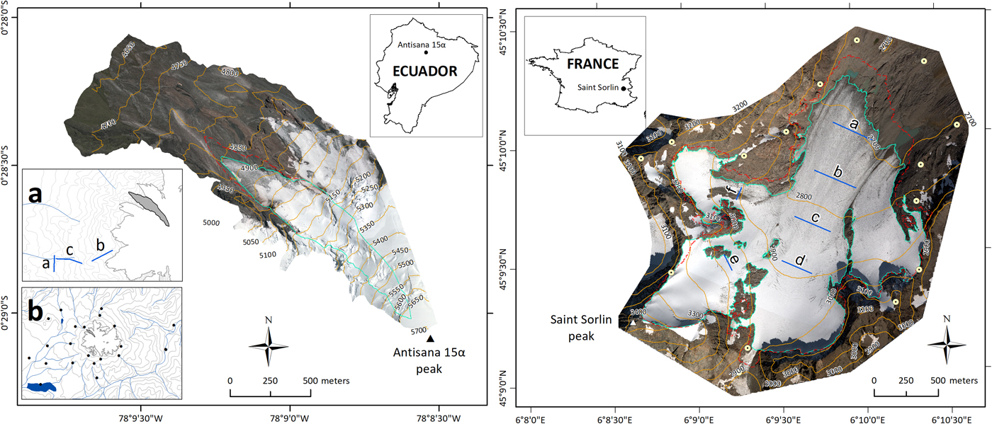
Fig. 1. On the left, Glaciar Antisana 15α (inset map of Ecuador, the black dot shows the location of the glacier), cyan and red lines are the outlines of the glacier in September 2009 and August 1997, respectively; 50-m interval contours are shown and the coordinates are given in degrees (reference data WGS84). Inset map (a) shows the DGPS cross-sections (a, b, c) located on the nonglacierized terrain used to assess the bundle block adjustment. Inset map (b) shows the location of the 21 GCPs used to perform the bundle block adjustment. On the right, Glacier de Saint-Sorlin (inset map of France, the black dot shows the location of the glacier), cyan and red line are the outlines of the glacier in September 2014 and August 2003, respectively; 100-m interval contours are shown and the coordinates are given in degrees (reference data WGS84). White circles show the location of the 15 GCPs used to carry out the bundle block adjustment and the blue lines show the six cross-sections used to assess the aero-triangulation.
Glaciar Antisana 15α located 40 km east of Quito (capital of Ecuador) in the Cordillera Oriental (0°28′S, 78°09′W). In 2009, its narrow shape covered an area of 0.27 km2. The ablation zone extends from 5050 m a.s.l. to 4800 m a.s.l. and has an average slope of ~30%, whereas the accumulation zone (from 5050 m a.s.l. to 5700 m a.s.l.) exhibits a very steep topography with an average slope of ~50%. Such a slope and the presence of several seracs and crevasses complicate the in situ collection of glaciological data. A monitoring program has been established to collect glaciological data since 1995 and meteorological data since 2004. Geodetic mass balance was determined between 1956 and 2009 as part of the same monitoring program (Basantes-Serrano, Reference Basantes-Serrano2015).
Glacier de Saint-Sorlin is located on the western side of the French Alps (45°10′N, 06°10′E). In 2014, the glacier extended over an area of 2.25 km2. The glacier has an average slope of ~30% and extends from 2650 m a.s.l. at its terminus to 3460 m a.s.l. Glaciological observations have been made since 1957 (Vincent and others, Reference Vincent, Vallon, Reynaud and Le Meur2000) whereas meteorological observations are only available since 2006 (Six and others, Reference Six, Wagnon, Sicart and Vincent2009).
More information about both glaciers is available through the GLACIOCLIM observatory (http://glacioclim.osug.fr/).
2.1. Aerial surveys and ground-control points (GCPs)
Aerial surveys over the Antisana volcano were conducted by the Instituto Geografico Militar (IGM, Ecuador) in August 1997 and September 2009. The aerial photos were acquired using a Leica RC30 metric camera, and the films scanned at 14 µm resolution using an Intergraph PhotoScan TD system. Aerial surveys of Glacier de Saint-Sorlin were conducted by the company SINTEGRA in September 2003 using a Leica RC30 metric camera (scanned at 14-μm resolution) and in September 2014 using a DMC II digital metric camera. The characteristics of the aerial photographs taken during each survey of the two glaciers are listed in Table 1.
Table 1. Characteristics of the aerial photographs and the bundle bock adjustment of the aerial surveys on the Antisana volcano and Saint-Sorlin glacier
* Indicates the master block.
For both glaciers, aero-triangulation, hereafter called ‘bundle block adjustment’, was performed using a geodetic network of GCPs established by interpreting rock features assumed to be stable from the imagery and measured using the static Differential Global Positioning Systems (DGPS) technique with centimetric precision in planimetry and altimetry. For Antisana, we used 21 GCPs measured in two campaigns in 2009 and 2011 (Fig. 1). For Saint-Sorlin, we used 15 GCPs measured between 1995 and 2015 (Fig. 1).
Additionally, as part of the monitoring programs, DGPS data were collected over several topographic profiles using the rapid static method. Three topographic profiles were captured in the nonglacierized western zone of the Antisana volcano and six topographic profiles on the Glacier de Saint-Sorlin 1 month before the 2014 aerial survey (Fig. 1). These geodetic data were used to validate the bundle block adjustment.
All photogrammetric tasks were carried out using Orima-DT software from Hexagon Geospatial®. The same photogrammetric workflow described in Basantes-Serrano and others (Reference Basantes-Serrano2016) for the Antisana Ice Cap was used for Glacier de Saint-Sorlin.
3. METHODS
In this section, we first describe the traditional methods used to compute changes in the surface elevation of the glaciers. We then present a new approach to densify the sampling points used to compute the glacier-wide elevation change.
3.1. Traditional method 1: dense manual restitution and sequential DEM differencing (SeqDEM)
First, sampling points were restituted manually over the entire surface of the glacier for each of the two aerial surveys following a discrete procedure. In view of the spatial resolution of the photography and the glacier topography (see Section 2), a full density photogrammetric restitution was performed using a regular grid with a sampling distance of 10 m for both glaciers. To improve DEM generation, some additional points were restituted on the glacier because of the presence of crevasses at the surface of the glaciers that were not fully captured by the 10-m grid. The DEM for each survey date was created based on the interpolation of the regular grid using a minimum curvature method.
Then, SeqDEMs were differenced to resolve the surface-elevation change from which the geodetic mass balance can be computed (Thibert and others, Reference Thibert, Blanc, Vincent and Eckert2008) by:
 $$Bgeod_{\lsqb {t_{\rm 0} - t_{\rm f}} \rsqb } = \displaystyle{{\bar \rho {\rm \;} \times {\rm \;} r^2 \times {\rm \;} \mathop \sum \nolimits_{i = 1}^p \Delta h(x)} \over {\bar S}}$$
where  $\bar \rho $ = 850 kg m−3 is the average density of the material associated with change in volume (Huss, Reference Huss2013), r is the pixel size, Δh is the glacier surface-elevation change for each locationx, p is the number of pixels covering the glacier at its maximum extent and
  $\bar S$ is the glacier surface area averaged over the period between the date of the first aerial survey t 0 and date of the second aerial surveyt f.
Despite the limitation associated with time and the difficulty involved in interpreting the whole glacier topography in areas of the image with insufficient contrast, the DEM differencing method using a complete dense manual restitution is considered sufficiently accurate to compute elevation changes over the entire surface of the glacier. In this study, the method is used as the reference to assess the reliability of the results of the two alternative approaches, whose aim is to reduce the time-consuming process of photogrammetric restitution.
3.2. Traditional method 2: selective profiling method (SePM)
Another way to capture changes in elevation in shorter time and at less financial cost is to select some topographic profiles to be restituted (or measured) along and/or perpendicular to the central flowlines of the glacier in an effort to cover most of the elevation range, yet avoiding areas with low contrast, shadows, seracs, or that are subject to frequent avalanches. The topographic profiles need to be restituted at the same location for each aerial survey in order to compute the changes in elevation.
The geodetic mass balance is estimated as follows: first, the glacier is divided into regular elevation bands and the mean surface area of each band at each geodetic survey is estimated. Second, topographic profiles are measured perpendicular to the central flowlines in each band, and the average elevation change is computed from each restituted topographic profile. When the topographic profiles are measured along the central flowlines, then the average elevation change is computed for the portion of the topographic profile located inside each band. The average elevation change is weighted by the relative mean surface area of each elevation band. When the topographic profiles cannot be measured because of complex patterns of elevation changes, a linear interpolation is used to extrapolate the trend observed in neighboring elevation bands.
Finally, the geodetic mass balance is computed from the area-weighted elevation change using an average density value of  $\bar \rho $ of 850 kg m−3 (Huss, Reference Huss2013).
3.3. Geodetic spatial sampling design (SSD) based on geostatistical analysis
In glaciology, geostatistical analysis has long been used to estimate glacier mass balance from point data obtained using the glaciological method (Hock and Jensen, Reference Hock and Jensen1999; Rotschky and others, Reference Rotschky2007; Cullen and others, Reference Cullen2017), mapping ice bodies (Stosius and Herzfeld, Reference Stosius and Herzfeld2004), detecting crevasses (Kodde and others, Reference Kodde, Pfeifer, Gorte, Geist and Höfle2007) or estimating the uncertainties in elevation differences in geodetic mass balances (Rolstad and others, Reference Rolstad, Haug and Denby2009; Magnússon and others, Reference Magnússon, Muñoz-Cobo Belart, Pálsson, Ágústsson and Crochet2016). Here, we use a geostatistical framework to guide the photogrammetric restitution toward new sampling sites where elevation measurements are needed. This approach was inspired by spatial sampling applied in other fields such as environmental, social and resource monitoring (Kish, Reference Kish1965; Jayaraman, Reference Jayaraman1999; Melles and others, Reference Melles2011; Wang and others, Reference Wang2013). For our application, the SSD strategy is applied iteratively using the ‘gstat’ and ‘rgdal’ packages in the open source R language for statistical computing (Pebesma and Wesseling, Reference Pebesma and Wesseling1998; Bivand and others, Reference Bivand, Pebesma and Gomez-Rubio2008). Figure 2 shows the workflow of the procedure, which is described as follows:
Fig. 2. Schematic overview of the SSD method.
3.3.1. Definition of the reference layer and its spatial characteristics
For the purpose of validation of the results of the new proposed approach, a reference layer must be defined. For that reference prediction layer we use the spatial structure of the elevation change obtained with the SeqDEM method. Thus, the experimental semi-variogram γ(l) of the reference layer is computed by:
 $$\hat \gamma (l) = {\rm \;} \displaystyle{1 \over {2N(l)}}\mathop \sum \limits_{i = 1}^{N(l)} \lsqb {{\lcub {\Delta h(x) - \Delta h(x + l)} \rcub }^2} \rsqb ,$$
where l denotes the lag distance between a pair of observations and N(l) the number of pairs of observations separated by lag l. To ensure that first and second order stationarity assumptions are met for semi-variogram computation and subsequent Kriging, the Δh measurements are de-trended using a two-dimensional hyperplane.
To choose the model of the spatial structure of our elevation change, we fit three theoretical semi-variogram models, namely spherical, exponential and Gaussian. The theoretical semi-variogram is defined by three parameters: the nugget parameter shows the bias of the predicted model which is partly explained by the error of the measure and partly by a random component which is not spatially dependent; the sill parameter is the sampled variance; and the range parameter is the distance at which Δh(x) and Δh(x + l) are spatially uncorrelated (Matheron, Reference Matheron1962; Cressie, Reference Cressie1988).
For each model, the prediction layer of the surface-elevation changeΔh is computed using universal Kriging, as well as its uncertainty referred to as the Kriging variance layer.
The performance of each model was assessed by applying a leave-one-out cross-validation (LOOCV) protocol based on Kriging predictions (Bivand and others, Reference Bivand, Pebesma and Gomez-Rubio2008). Cross-validation is a process in which a known observation is removed and its value is predicted using the other points. The predicted elevation change is compared with the observation and the root mean square error of the residuals, RMSE, is used as a selection criterion:
 $${\rm RMSE} = {\rm \;} \sqrt {\displaystyle{{\mathop \sum \nolimits_{i = 1}^n {(\widehat{{\Delta h}}(x) - \Delta h(x))}^2} \over n}}, $$
where Δh(x) and  $\widehat{{\Delta h}}(x)$ are the reference and predicted elevation changes at location x i, respectively and n is the number of points in the full density restitution. Finally, the model with the lowest RMSE is selected to fit the spatial structure of our reference dataset and its parameters can be computed: nugget, sill and range. The selected theoretical model was also used to fit the spatial structure for all the other test cases to facilitate comparison.
3.3.2. SSD method, initial point cloud
We arbitrarily define an initial number of 50 sampling points. Their initial locations are selected following a simple random sample approach and each sampling location x is photogrammetrically restituted for each aerial survey and the elevation difference is computed at each point.
Following the same procedure as above, we compute the experimental semi-variogram of our initial point cloud and then fit the theoretical model. Next, the initial Kriging prediction and its Kriging variance layer are computed using the universal Kriging technique. This prediction is a first approximation of the elevation difference over the whole glacier surface. A LOOCV is performed to evaluate the quality of the prediction of the elevation changes.
3.3.3. SSD method, sampling network densification
Based on the Kriging variance layer, we identify the locations with a large prediction error to inform the sites to add new sampling points. From locations outside the 75th percentile of the variance, we randomly select 50 additional sites to be measured according to the criterion of the analyst who will decide, based on his/her own expertise, if the locations are suitable to measure additional sampling points to quantify the mass balance (i.e. have a minimum snow cover or shadows, optimal brightness and contrast in the photos). The set of 50 new points is merged with the previous set and the procedure is repeated (i.e. quantification of the semi-variogram, etc.).
In order to stop the iterative process and to compute the glacier-wide elevation change, the standard error of the prediction is taken as a criterion. Finally, the resulting surface-elevation changes provided by the prediction layer can be used to estimate the geodetic balance according to Eqn (1).
3.4. Uncertainty of the predicted surface-elevation changes
For the SeqDEM method, the uncertainty of elevation difference σ A is computed using Eqn (14) in Rolstad and others (Reference Rolstad, Haug and Denby2009). The estimation integrates the uncertainty of the DEM differencing on stable terrainσ Δh, the glacier surface area at the first survey dateA and the area over which there is a spatial correlation $\; A_{{\rm cor}} = \pi a_1^2 $, with
  $a_1^2 $ being the lag distance where a spatial correlation exists. A comprehensive description of the way to compute uncertainties is given in Fischer and others (Reference Fischer, Huss and Hoelzle2015).
Because this paper focuses on the computation of the glacier-wide elevation changes, the uncertainty about the density used for conversion to mass does not need to be taken into consideration. We also disregard random errors associated with basal and internal ablation or accumulation. The reliability of the surface-elevation changes produced by the SePM and SSD methods is assessed by comparing the layers predicted by each method with the reference layer of the SeqDEM method. Here, the RMSE of the residuals is considered as a measure of accuracy.
4. RESULTS
4.1. Spatial consistency of the photogrammetric blocks
Completing the bundle block adjustment enabled a stereoscopic model to be viewed in 3-D that allows geometric features of the surface topography to be measured by photogrammetric restitution. To avoid misalignment between two photogrammetric blocks, it is recommended to use the same control network in all the stereographic models (Cox and March, Reference Cox and March2004). Our geodetic reference relied on the GCP network located around the glaciers and was used for the adjustment of all the photogrammetric blocks (Fig. 1).
In the aero-triangulation, the triangulation residuals for Antisana aerial surveys were <0.30 m. For Saint-Sorlin, the accuracy of the aero-triangulations was <0.20 m for the 2003 aerial survey and <0.10 m for the 2014 aerial survey. This difference in the accuracy of the aero-triangulation for Saint-Sorlin can be explained by the type of aerial sensor used to acquire the aerial photos. For the aerial photos taken before 2010, a RC30 was used but uncalibrated lens distortions had to be resolved during the absolute orientation process, whereas the aerial photos taken in 2014 of Glacier de Saint-Sorlin, a DMC panchromatic digital sensor was used which is free of geometric distortions.
To validate the spatial consistency of each photogrammetric block in the two glaciers, we used 91 independent checkpoints distributed along several topographic profiles acquired during the DGPS survey and re-measured by photogrammetry on each photogrammetric block (Fig. 1 and Table 1). The vertical biases of the two glaciers are of the same order of magnitude. For Glaciar Antisana 15α, the vertical comparison yields an average residual of −0.50 m (RMSΔh = 1.40 m) for the photogrammetric models. Basantes-Serrano and others (Reference Basantes-Serrano2016) estimated the changes in elevation in 18 sites measured on the flat dome-shaped summit in the upper reaches of the volcano (0.15 km2) from 1997 to 2009. These authors confirmed that the bias in elevation changes in the upper part of the glacier is within the geodetic uncertainties (RMSΔh = 1.5 m). A similar assessment was made for Glacier de Saint-Sorlin, yielding an average residual of −0.52 m (RMSΔh = 0.66 m). For the 2014 aerial block, the topographic profiles located below 2850 m a.s.l. (i.e. profiles a, b, c in Fig. 1) led to an average residual of −0.40 m (RMSΔh = 0.51 m), whereas from this elevation up to the summit (i.e. profiles d, e, f in Fig. 1) the average residual was −0.81 m (RMSΔh = 0.92 m). For the 2003 aerial block, the topographic profiles located below 2900 m a.s.l. (i.e. profiles a, b, c, d in Fig. 1) had an average residual of 0.01 m (RMSΔh = 0.40 m) and from 2900 m a.s.l. up to the summit (i.e. profiles e and f in Fig. 1) the average residual was 0.45 m (RMSΔh = 1.16 m). This difference can be explained by the time difference between the geodetic surveys, that is ~1-month between the DGPS measurements in 2003 and 2014 (i.e. 21 August 2003 and 20 August 2014) and the date of the aerial survey (i.e. 20 September 2003 and 27 September 2014). Also, a mean ablation of ~0.65 m w.e. obtained by direct mass balance measurements between 2700 m a.s.l. and 2800 m a.s.l. close to the date of the geodetic observations confirms this observation. Thus, the discrepancies are within the geodetic uncertainties.
In order to assess the consistency of the DEMs (i.e. 1997/2009 for Glaciar Antisana 15α glacier and 2003/2014 for Glacier de Saint-Sorlin), we compared elevations on the stable terrain surrounding the glaciers (Fig. 3). The average of the residual was 0.05 m for Glaciar Antisana 15α and 0.16 m for Glacier de Saint-Sorlin, and a standard error of 0.03 m (5131 pixels) and 0.02 m (18 700 pixels), respectively. Given the limited bias between the DEMs, we did not need to perform 3D co-registration of the successive DEMs, as recommended by Nuth and Kääb (Reference Nuth and Kääb2011).
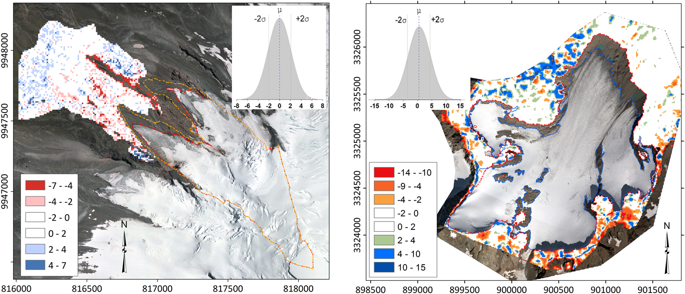
Fig. 3. Surface-elevation changes (m) on the glacier foreland: for Glaciar Antisana 15α [DEM1997⋀DEM2009] on the left, and Glacier de Saint-Sorlin [DEM2008⋀DEM2014] on the right, with respectively 5131 and 18 700 pixels (spatial resolution = 10 m). The normal distribution, mean and two std dev. of the elevation changes are shown in the inset graph.
4.2. Quantification of the surface-elevation changes
Table 2 presents the results of the different methods and Table 3 presents the total number of sampling points that differed considerably from one method to another.
Table 2. Mean surface-elevation changes  $\overline {{\rm \Delta} h} $ and in m computed by the different methods for Antisana 15α glacier from August 1997 to September 2009 and for Saint-Sorlin glacier from September 2003 to September 2014
* Indicates the reference values for both glaciers with the related random uncertainty. The uncertainty for the SePM methods and the SSD approach is the RMSE of the residuals of the comparison with the reference.
Table 3. Number of sampling points measured on each glacier with each method
Using the conventional DEM differencing method, the average surface elevation was −2.07 ± 0.29 m and −16.95 ± 1.07 m for Glaciar Antisana 15α and Glacier de Saint-Sorlin, respectively. These results were obtained with a large number of sampling points (10-m grid size), which will depend on the size of the glacier concerned and the amount of contrast in the images of the surface.
The difference in the glacier-wide elevation changes computed by the SePM method and the DEM differencing ranged from 0.30 m to 3.00 m. When the topographic profiles along the central flowline were applied on these glaciers, <30 restituted points were measured (Figs 4a, b) and when the topographic profiles perpendicular to the central flowline were applied, <90 restituted points were measured (Figs 4c, d).
Fig. 4. Topographic profiles along (a and b) and perpendicular (c and d) to the central flowline used to compute changes in thickness for Antisana 15α and Saint-Sorlin glaciers using geodetic measurements. The gray dashed lines are the outlines of the glacier in September 2009 and August 1997 for Antisana 15α and the outlines of the glacier in September 2014 and August 2003 for Saint-Sorlin.
When the SSD method was used, we first defined the spatial structure of the full density glacier topography as our reference layer. Three theoretical models were assessed and a RMSE of the residuals of 2.98 m (1.05 m) for Antisana 15α (Saint-Sorlin) showed that the exponential model outperformed the other theoretical models and provided the best predictions (Fig. 5 and Table 4). This was supported by the correlation between the measured elevation changes and the predicted elevation changes (r 2 >0.80 at p < 0.01 for the three models, Table 4). Thus, during the iterative process, the exponential model was used to determine the Kriging variance of the prediction.
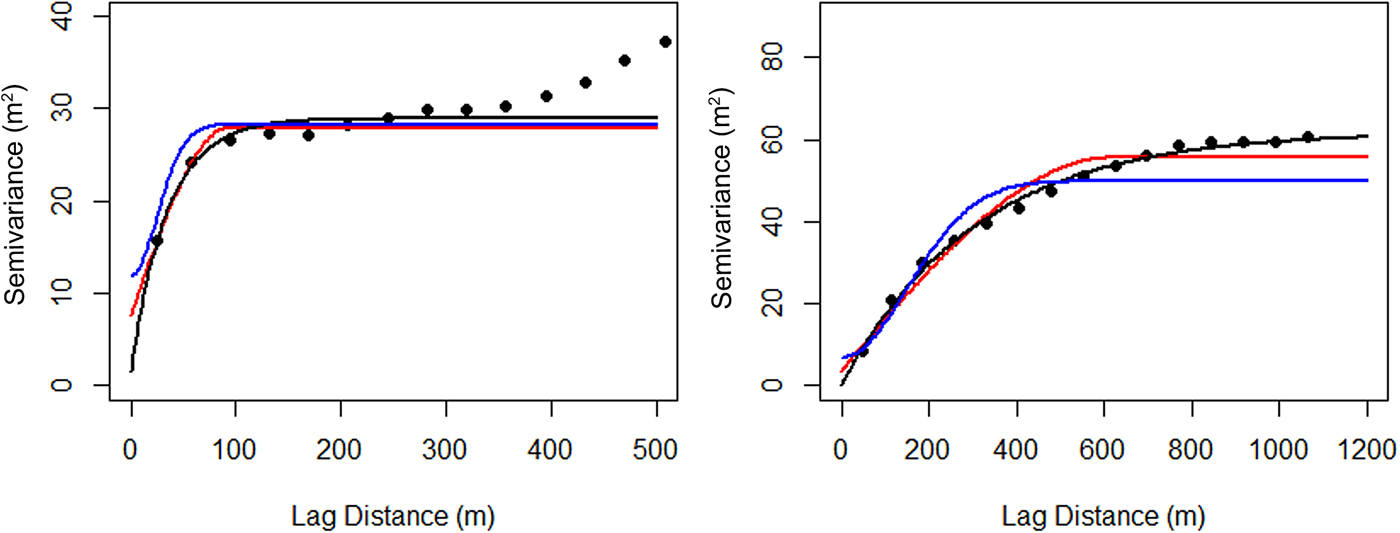
Fig. 5. Experimental semi-variogram (black circles) and fitted theoretical models: spherical (red), exponential (black), and Gaussian (blue); for the two glaciers (Antisana 15α on the left and Saint-Sorlin on the right). The parameters of each theoretical semi-variogram are listed in Table 4.
Table 4. Quality of the predictions by the three semi-variogram models for (a) Glaciar Antisana 15α and (b) Glacier de Saint-Sorlin
Then, the first iteration was completed using 50 sampling points randomly distributed over the surface of the glacier. After each iteration, a new set of 50 points was added in areas with high variance. For our experiment, the iterations continue until a full grid of 10-m was constructed. For example, the Antisana 15α is modeled at full density with 3160 points, thus allowing ~65 iterations. In the case of Saint Sorlin-the process stopped at ~555 iterations to reach the full density of 27 816 points.
Although the parameters of the model varied substantially over a number of iterations; they converged relatively rapidly to values approaching those of the full-resolution dataset (Fig. 6). Based on the changes in variance, we found that ~50 iterations are sufficient for the spatial structure of the elevation change to converge toward that of the reference dataset (Fig. 6) resulting in glacier-wide elevation changes very close to the result computed by the DEM differencing method (difference <0.04 m).
Fig. 6. Changes in the parameters of the semi-variogram model as a function of the number of iterations for (a) Glaciar Antisana 15α and (b) Glacier de Saint-Sorlin.
Figure 7 shows the solution of the exponential semi-variogram model and the adjusted parameters for the full density topography and for the 1st and 50th iterations on the two glaciers. For Antisana 15α, 60% of the sill was reached within a lag distance of 35 m; after which the spatial auto-correlation decreased and reached 95% of the sill at a range of 104 m; for Saint-Sorlin, the semi-variogram reached 60% of the sill at a lag distance of 306 m and 95% of the sill at a range of 917 m. This confirms that the change in the spatial structure of elevation was well captured by a significantly reduced subset of measurements.
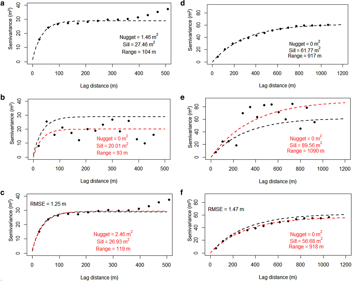
Fig. 7. Experimental semi-variogram (black circles) and fitted exponential model for the two glaciers (Antisana 15α on the left and Saint-Sorlin on the right): the black dashed line stands for the full density topography in (a) and (d); the red dashed line stands for the 1st iteration in (b) and (e) and for the 50th iteration in (c) and (f). The parameters of each semi-variogram model are included (nugget; sill and range). The RMSE from the comparison between the reference elevation change from DEM differencing and the estimated elevation change from the SSD method is shown in graphs (c) and (f).
5. DISCUSSION
5.1. Spatial variability of the elevation changes
Changes in the spatial variability of elevation over the entire surface of the glacier were captured by the full density topography of the SeqDEM method. However, the data collection often misses parts of the glacier surface because of poor photographic contrast, and is impaired by the time-consuming process associated with the systematic manual restitution of a dense grid.
For the SePM method, a semi-variogram analysis of the topographic profiles revealed a noticeable scatter around the fitted model (Fig. 8), while LOOCV analysis showed significant residual values with a RMSE ranging from 5 to 10 m. Thus, this method is not able to fully resolve the spatial variability of the elevation changes over the entire surface of the glacier. This could be due to the small sample size and the location of the sampling points.
Fig. 8. Experimental semi-variogram and fitted exponential model for the topographic profiles measured for the two glaciers (Antisana 15α on the left and Saint-Sorlin on the right): black circles and black dashed line correspond to perpendicular profiles and gray circles and gray dashed line correspond to profiles along to the central flowline. The RMSE from the cross-validation process for the profiling method is given in each graph.
The SSD method relies on a Kriging technique to predict changes in elevation over the whole surface of the glacier using a semi-variogram model, as well as resolving areas of higher uncertainty that could compromise the estimated geodetic balance. To verify the ability of the iterative SSD method to capture the spatial structure of our data, we compared the fitted semi-variogram of the full density topography (i.e. the reference layer) and the semi-variograms of the successive iterations (Fig. 7).
The aim of the first few iterations is to resolve the global trend and capture some, although not all, local variability of the elevation change; while the iterative densification allows the small-scale spatial structure to be progressively refined (Fig. 6). As could be expected, the first few iterations result in a significantly dispersed semi-variogram due to the small sample size, and failure to capture the spatial variability of elevation change to a degree that would compromise the geodetic balance estimate.
Figure 6 shows how the spatial variability of the surface-elevation changes quickly converges toward that of the full dataset. One can see how the key characteristics of the semi-variogram (i.e. nugget, sill and range) converge rapidly close to the value of the reference semi-variogram, when the global variance of the surface-elevation change is resolved (Fig. 7). In addition, Fig. 9 illustrates how the standard error of the prediction  $({\rm SE} = (\sigma /\sqrt n ))$ decreases logarithmically with the number of iterations or sampling points. Thus, we consider that when the standard error change marginally, i.e. after ~50 iterations or ~2500 restituted points, we halted the iterative process and the glacier-wide elevation change can be computed for both glaciers.
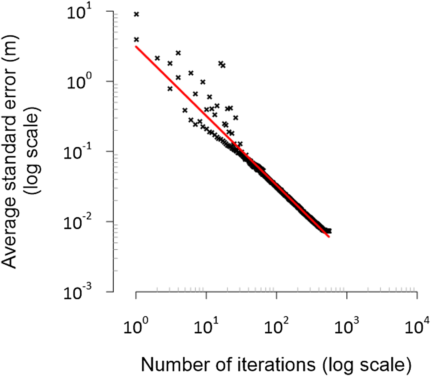
Fig. 9. Average standard error as a function of the number of iterations (log scale). Black crosses are the values for the two glaciers. The red line shows the decreasing logarithmic function fitted to the data.
5.2. Spatial representativeness of the elevation changes
To assess whether the spatial variation of the elevation changes on the glacier is well captured by each approach, we analyzed the rate of elevation changes with altitude along the central flowline (Fig. 10).
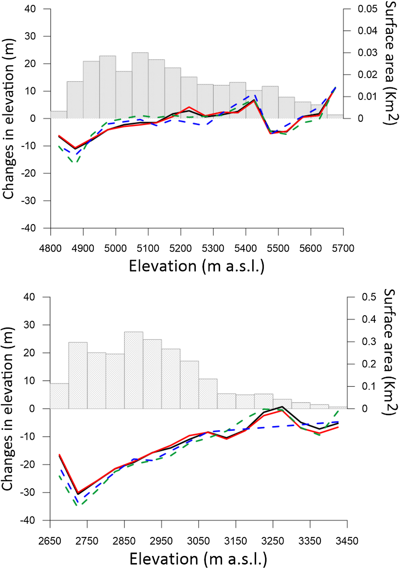
Fig. 10. Hypsometry (gray histogram) and changes in elevation vs altitude for (a) Glaciar Antisana 15α over the period 1997–2009; and (b) Glacier de Saint-Sorlin over the period 2003–2014. The variation in elevation was averaged for each 50-m elevation band. The changes in elevation extracted by the different approaches are shown: SeqDEM (solid black line), profiles along the central flowline (green dashed line) and perpendicular (blue dashed line) to the central flowline and geo-statistical analysis (red line).
All three methods are capable of providing an approximation of the altitudinal gradient of elevation changes. This is consistent with evidence from previous studies (i.e. Echelmeyer and others, Reference Echelmeyer1996; Arendt and others, Reference Arendt, Echelmeyer, Harrison, Lingle and Valentine2002; Vincent and others, Reference Vincent2013). However, there are some local differences between the shape obtained by the SeqDEM method and the shape obtained by the SePM method: the SePM method tends to overestimate the ice losses in the lower reaches of the glaciers by ~20%. This could be due to the low density of the sampling of points used to compute the elevation change. The comparison of these curves with the reference curve (SeqDEM) revealed significant discrepancies in the profiling method: for Glaciar Antisana 15α, the mean difference was 0.40 m (RMSE = 2.25 m) whereas for Glacier de Saint-Sorlin, the mean difference was 1.35 m (RMSE = 3.06 m) (Fig. 10).
Figure 11 shows the spatial distribution of the changes over the whole surface of the glacier. The SSD method can reliably reproduce the spatial variability of the elevation changes computed by SeqDEM: for Glaciar Antisana 15α the mean difference was 0.01 m (RMSE = 1.25 m) and for Glacier de Saint-Sorlin, the mean difference was 0.03 m (RMSE = 1.40 m). Figure 12 shows how the sampling points tend to be concentrated in the areas with significant changes (Fig. 11). In the ablation zone of the Glaciar Antisana 15α (average slope of ~35%), the elevation changes show a homogeneous ice thinning of ~20 m, here ~22% of the sampling points are concentrated (i.e. below 5050 m a.s.l.). Above 5050 m a.s.l., ~60% of the sampling points are located in the very steep accumulation areas where a complex and heterogeneous pattern of elevation changes appear (i.e. slope between 40% and 80%). This zone represents a ~62% of the glacier surface-area.
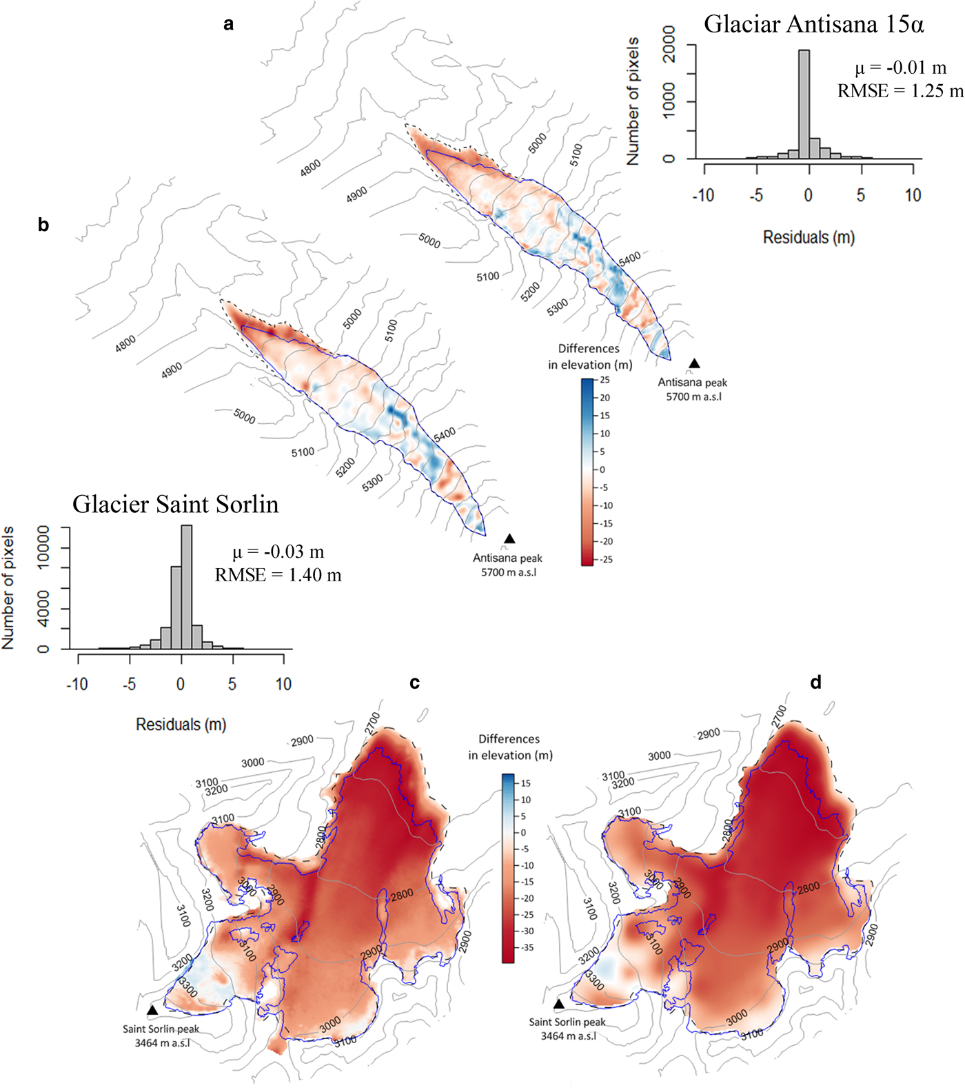
Fig. 11. Spatial variability of the changes in surface elevation (in m) resulting from the SeqDEM technique (a and c) and from the geostatistical framework at the 50th iteration (b and d). (a) and (b) show Glaciar Antisana 15α, the black dashed line shows its extension in 1997 and the blue line in 2009, 50 m interval contours are shown. (c) and (d) show Glacier de Saint-Sorlin, the black dashed line shows its extension in 2003 and the blue line in 2014, 100 m interval contours are shown. The color scale shows the decline in surface elevation (from pale to dark red) or the rise (from pale to dark blue). The inset histogram shows the histogram of distribution of the residuals between the SeqDEM layer and the SSD layer.
Fig. 12. Distribution of the sampling points as a function of the slope for the glacier Antisana 15α and Glacier de Saint-Sorlin.
For the Glacier de Saint-Sorlin, the ice thinning can be seen all over the surface, decreasing almost regularly from the lower reaches of the glacier where the thinning reached ~35 m to the upper reaches where it is close to 0. Here, 36% of the points are located on areas with gentle slope (i.e. slope between 0% and 20%) from the glacier front to 3000 m a.s.l.; and ~39% of the points are located on the sloping areas (i.e. slope between 20 and 40%) which represents a ~40% of the glacier surface-area, and 25% of the sampling points are distributed in the upper reaches of the glacier.
5.3. Space sensitivity of the SSD method in determining the elevation change
With the SeqDEM method, measuring a large number of isolated points covers the glacier surface almost exhaustively, thus ensuring that the interpolated DEM reliably represents the glacier topography. As a consequence, much more time is required for this systematic procedure than for the other methods. This is practical when automated point extraction performs well but not when it fails due to poor contrast, as is often the case over the glaciers. In such cases, the technical expertise of the operator plays an important role in the ability to interpret the glacier surface. We thus estimate that an experienced operator can manually digitalize 1000 elevation points in one 4-h session of photogrammetric restitution. If one 4-h session is accomplished per day, one operator would need between 6 and 28 days to measure each of the two stereoscopic models in our example by photogrammetry.
The two other methods (i.e. profiling method and geostatistical analysis) seem to be suitable alternatives because the total number of the elevation points is significantly reduced as is the time dedicated to the photogrammetric restitution. However, the total number and the location of the points used by the profiling method seem to be insufficient to provide an accurate representation of the spatial variability of the ice mass changes, and this can affect the total estimation of the glacier-wide mass balance (Fig. 10).
The SSD method appears to provide more conservative results based on the stabilization of the variance of the surface-elevation change toward the 50th iteration (i.e. ~2500 sampling points) with the advantage of resolving most of the spatial variability without compromising the accuracy of the results. Based on this analysis, for this total amount of sampling points, a grid resolution of 10 m × 10 m is suitable for mapping surface-elevation change on the Glaciar Antisana 15α (<1 km2), whereas for Glacier de Saint Sorlin (~2.5 km2) a 30-m grid size seems to be appropriate.
In order to assess the generalization of our results to other types of glacier, we performed a test on the Glacier de la Mer de Glace located in the Mont-Blanc massif, a largest glacier in the French Alps (~30 km2). This glacier presents a complex morphology including several tributaries with an elevation range between 4300 m a.s.l. in the accumulation area and 1500 m a.s.l. in the front of the glacier (Vincent and others, Reference Vincent, Harter, Gilbert, Berthier and Six2014). Based on the conventional SeqDEM approach, Rabatel and others (Reference Rabatel, Dedieu and Vincent2016) computed an average surface-elevation change of −16.94 m using two DEMs of 20-m grid resolution derived from SPOT5 stereo pairs acquired on 8 August 2003 and 15 October 2011. When the SSD method is applied, the glacier-wide elevation change is only 0.10 m more negative (RMSE = 4.58 m).
As for the two other cases illustrated in this study, ~50 iterations were needed to get the stabilization of the semi-variogram parameters and the spatial variability of the surface-elevation change to be captured (Fig. 13). For this experiment only 100 iterations were run. This final assessment confirms the replicability of our methodology to be applied to other mountain glaciers with different morphological characteristics.
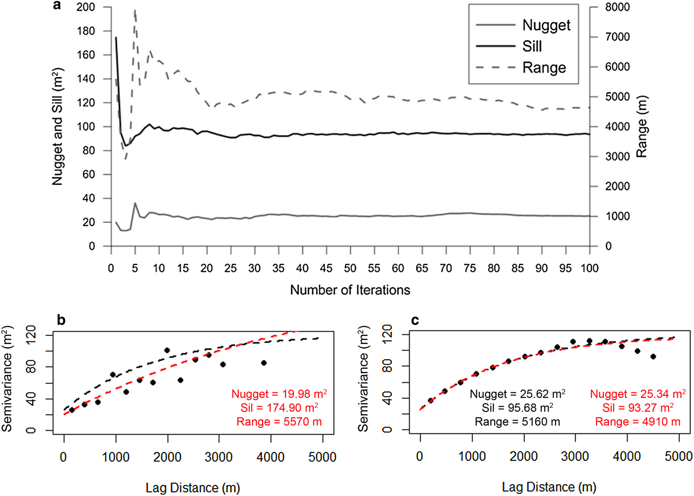
Fig 13. (a) Stabilization of the parameters of the semi-variogram model as a function of the number of iterations of Mer the Glace; and Experimental semi-variogram (black circles) and fitted exponential model of Mer de Glace: the black dashed line stands for the full density topography and the red dashed line stands for the 1st iteration in (b) and for the 50th iteration in (c). The parameters of each semi-variogram model are included.
6. CONCLUSIONS
In this study, we provided a rational and a very robust framework to optimize the quantification of the glacier-wide mass balance. Our methodological framework takes into account the spatial variability of the glacier elevation changes to guide an appropriate collection of a subset of geodetic measurements over optimal areas by avoiding sites where manual or automatic stereo-matching is particularly challenging due to poor contrast in the stereo-images. In this context, we analyzed the performance of current approaches to compute a geodetic mass balance. The SeqDEM method is frequently regarded as a primary source to compute elevation differences on glaciers. However over glacierized area regions of low contrast are a limit for the DEM generation through the stereo-matching techniques. In this scenario, the manual restitution may be an alternative, but time-consuming. A faster alternative is the surface-elevation profiling method (SePM) approach, which can be used for a preliminary approximation of the surface change gradient but does not provide a complete picture of the distribution of the ice glacier surface-elevation changes. Our results confirm that this method fails to capture the spatial distribution of the elevation changes and tends to overestimate ice losses in the lower reaches of the glacier. For our glaciers, this overestimation was ~20%.
Based on the semi-variogram analysis of the surface-elevation changes observed for three mountain glaciers with different morphological characteristics under different climate conditions, we tested a geostatistical framework to optimize the quantification of the geodetic mass balance. We show that our approach can accurately reproduce the overall shape of the elevation change with considerably fewer geodetic measurements than a fine systematic grid, meaning a significant reduction in the time dedicated to the data collection procedure.
Our results highlight the high potential of our methodological framework to contribute to fill the gap of mass balance series at a decadal scale on mountain glaciers with different morphological characteristics and subject to different climate conditions. In order to apply our methodological framework, we recommend:
1. Measuring a minimum of ~2500 sampling points per glacier to estimate a glacier-wide elevation change with a high enough accuracy to satisfy glacier mass balance studies.
2. Evaluating the evolution of the standard error of the prediction as a criterion to stop the iterative process. The iterative process can be halted when the standard error change marginally, and the glacier-wide elevation change can be computed.
ACKNOWLEDGEMENTS
Rubén Basantes acknowledges the support of the Centro de Estudios Científicos (CECs) funded by the Centers of Excellence Base Financing Program of the Comisión Nacional de Investigación Científica y Tecnológica (CONICYT-Chile). This study was conducted in the framework of the Service National d'Observation GLACIOCLIM (http://glacioclim.osug.fr/) and the Laboratoire Mixte International GREAT-ICE (http://www.great-ice.ird.fr/) with the support of the LabExOSUG@2020 (Investissements d'avenir – ANR10 LABX56). The authors are grateful to the CNES/SPOT-Image ISIS program contract # 2011-513 for providing the SPOT images and SPOTDEM from 2003 to 2011. Pascal Sirguey acknowledges the University of Otago, the Grenoble Institute of Technology (Grenoble-INP) and the University Grenoble-Alpes (UGA) for supporting his contribution to this work while on research and study leave in Grenoble.


 Open access