Estimation of Glacier Thickness From Surface Mass Balance and Ice Flow Velocities: A Case Study on Argentière Glacier, France
 Antoine Rabatel
 Olivier Sanchez
 - Univ. Grenoble Alpes, CNRS, IRD, Grenoble-INP, Institut des Géosciences de l'Environnement (UMR 5001), Grenoble, France
Glacier thickness distribution is a prerequisite to simulate the future of glaciers. Inaccurate thicknesses may lead to significant uncertainties in the timing of future changes to glaciers and their consequences for water resources or sea level rise. Unfortunately, glacier thickness distribution is rarely measured and consequently has to be estimated. In this study, we present an approach developed on the well documented Argentière Glacier (French Alps) that uses surface mass balance (SMB) together with surface flow velocity data to quantify glacier thickness distribution over the entire surface of the glacier. We compare the results of our approach to those obtained applying Farinotti et al. (2009) approach. Our results show that glacier thickness distribution are significantly biased when the glacier SMB profile used to quantify the ice fluxes is not constrained with in situ measurements. We also show that even with SMB measurements available on the studied glacier, ice flux estimates can be inaccurate. This inability to correctly estimate ice fluxes from the apparent SMB may be due to the steady state assumption that is not respected from the available glacier surface topography data. Therefore, ice thickness measurements on few cross sections (four are used in this study) are required to constrain the ice flux estimates and lead to an overall agreement between the ice thickness estimations and measurements. Using our approach, the ice thicknesses only differ by 10% from observations in average, but can differ by up to 150 m (or 30%) locally. We also show that approaches that use the glacier surface slope can lead to large uncertainties given that the quantification of the slope is highly uncertain. The approach presented here does not pretend to be applied globally but rather as a tool to quantify ice thickness distribution over the entire surface of glaciers for which a few in situ surface mass balance and thickness data are available together with surface flow velocities that can be obtained for example from remote sensing.
Introduction
Several approaches of differing complexity have been developed to simulate past, current or future changes of mountain glaciers by modeling the surface mass balance and the ice dynamics (e.g., Bindschadler, 1982; Hubbard et al., 1998; Oerlemans et al., 1998; Gudmundsson, 1999; Le Meur and Vincent, 2003; Sugiyama et al., 2007; Huss et al., 2010; Jouvet et al., 2011; Linsbauer et al., 2013; Vincent et al., 2014; Réveillet et al., 2015). Whatever the modeling approach used, the absence of accurate estimations of ice thickness over the entire surface of the glacier is the main constraint to accurately simulating future changes (e.g., Linsbauer et al., 2013; Beniston et al., 2018; Vuille et al., 2018). However, except on small glaciers with a gentle topography, it is almost impossible to measure the ice thickness through in situ observations over an entire glacier, regardless of the method used (e.g., hot water drilling, seismic or radar measurements, gravimetry). Thus, for the great majority of glaciers for which thickness measurements are available, these measurements were made along transverse profiles and then extrapolated to estimate thicknesses in unsurveyed areas (e.g., Fischer, 2009). Unfortunately, the number of surveyed glaciers is small: the recent GlaThiDa initiative gathers information on about 2,000 glaciers worldwide (WGMS, 2016), which represents ~1% of the number of glaciers included in the global inventories (GLIMS, 2013; Pfeffer et al., 2014). As a consequence, methods have emerged to estimate the ice thicknesses over the entire glacier surface that take advantage of the progressive increase in the availability of morpho-topographical data (glacier inventories, digital elevation models of the glacier surface), as well as glaciological data (surface mass balance, surface flow velocities) and point thickness measurements to calibrate parameterizations. Within the context of the Ice Thickness Models Intercomparison eXperiment, so-called ITMIX, conducted in the framework of the Working Group on Glacier Ice Thickness Estimation of the International Association of Cryospheric Sciences (IACS, http://cryosphericsciences.org/), Farinotti et al. (2017) presented a review of existing methods currently used to estimate ice thicknesses together with the results of the first intercomparison experiment in which no prior knowledge on thickness data was available. Seventeen approaches were tested. Some rely on: (1) a parameterization of the basal shear stress (e.g., Haeberli and Hoelzle, 1995; Linsbauer et al., 2012); (2) the principle of mass conservation and ice flow taking into account a varying number of input variables such as a digital elevation model (DEM), surface mass balance, surface flow velocity (e.g., Driedger and Kennard, 1986; Huss et al., 2008; Farinotti et al., 2009; Morlighem et al., 2011; Huss and Farinotti, 2012; Li et al., 2012; van Pelt et al., 2013; Brinkerhoff et al., 2016; Fürst et al., 2017); or (3) the use of artificial neural networks (Clarke et al., 2009).
Here, we propose an approach that combines (1) satellite-derived field and in situ measurements of glacier surface flow velocity, and (2) glacier surface mass balance measurements to retrieve ice thicknesses over the entire surface area of the glacier. The main differences with other approaches that use both surface mass balance and flow velocity data are: (1) no explicit ice flow model is needed in our approach conversely to Morlighem et al. (2011), van Pelt et al. (2013), or Fürst et al. (2017), for example; or (2) no temporal surface elevation changes are needed conversely to McNabb et al. (2012), for example. In addition, approaches based on the glacier surface slope (e.g., Farinotti et al., 2009; Huss and Farinotti, 2012; Linsbauer et al., 2012) have been largely used in recent studies as they need a limited number of input data and are straightforward to implement. However, the first round of ITMIX (Farinotti et al., 2017) has shown that such simple approaches do not accurately represent the glacier ice thickness distribution which is an issue for future glacier evolution modeling.
After providing a description of the proposed framework, we report on its application on Argentière Glacier in the French Alps, and how the results compare with those obtained from in situ measurements or using the approach proposed by Farinotti et al. (2009) and Huss and Farinotti (2012).
Study Site and Data
The methodological framework presented in this study was developed on Argentière Glacier (Figure 1) located in the Mont-Blanc range, French Alps (45°55′ N, 6°57′ E). An extensive description of the monitoring of this glacier conducted within the GLACIOCLIM observatory can be found in Vincent et al. (2009). Here we summarize the basic information. In 2003, this north-west facing glacier had a surface area of 12.4 km2, a length of about 10 km, and extended from an altitude of 3,400 m a.s.l. at the upper rimaye to 1,600 m a.s.l. at the snout. The glacier is free from rock debris except on the lowermost part of the tongue below the icefall located between 2,000 and 2,400 m a.s.l.
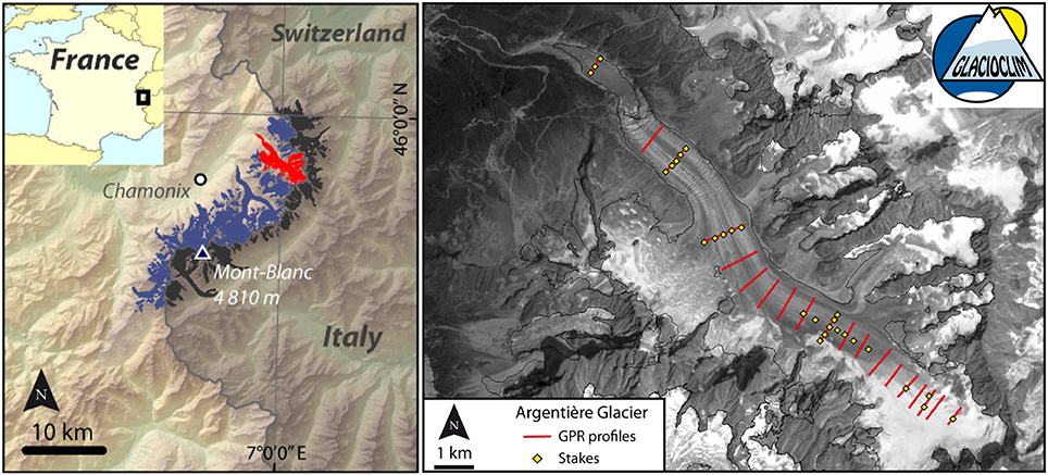
Figure 1. (Left) location of Argentière Glacier (Mont-Blanc Massif, French Alps). (Right) Field measurements of glacier thickness (seismic and radar) are in red. The yellow diamonds show the location of the stakes used to measure the surface mass balance and surface flow velocities.
Surface Mass Balance Data
The annual surface mass balances were monitored in the ablation area between 1975 and 1995, using 20 to 30 ablation stakes. Since 1995, winter and summer surface mass balance measurements (in early May and late September, respectively) have been performed and about 40 sites have been selected both in ablation and accumulation area (Figure 1). The point annual surface mass balance usually ranges from about 2 m w.e. yr−1 in the accumulation area to about −10 m w.e. yr−1 close to the snout. The equilibrium-line altitude (ELA) has been close to 2,850 m a.s.l. on average over the last 30 years (Rabatel et al., 2013, 2016).
In situ Ice Thickness Data
The first ice thickness measurements on Argentière Glacier were made in the 1950s (Reynaud, 1959). Then, in the 1970s, a hydroelectric power company (Emosson S.A.) planned to collect subglacial water. For this purpose, the bedrock topography was determined using seismic soundings at 4 cross-sections in the ablation zone located at 1,850, 2,400, 2,500, and 2,700 m a.s.l. (see the cross-sections where the ablation stakes transects are located in Figure 1). Additionally, eight and 24 boreholes were drilled on cross-sections located at 1,850 and 2,400 m a.s.l., respectively, to check the seismic results (Hantz, 1981; Vincent et al., 2009). The comparison showed differences that reached 30 m locally. To extend the information on the bedrock topography, ice thickness measurements were acquired on 15 additional profiles using ice penetrating radar (IPR) during field campaigns in January 2013, February-March 2014, and April 2015 (Figure 1). Our IPR is a geophysical instrument specially designed by the Canadian company Blue System Integration Ltd in collaboration with glaciologists to measure the thickness of glacier (Mingo and Flowers, 2010). It comprises a pair of transmitting and receiving 4.2 MHz antennas that allow continuous data acquisition, with data georeferenced using a GPS receiver.
Surface Flow Velocity Data
Surface flow velocities were quantified by measuring stake displacements at the end of the ablation season (September) using topographic methods (Vincent et al., 2009). Five to ten ablation stakes were placed on each cross-section for this purpose. In addition, painted stones were used to complete the measurement network and to determine the surface flow velocities on the longitudinal flow line passing through the center of each cross-section. To complete the spatial coverage of surface flow velocities, results obtained by Berthier et al. (2005) using a correlation method and SPOT5 satellite images from the year 2003 were used (Figure 2). We briefly summarize the method and results here, but refer the reader to Berthier et al. (2005) for a more complete description. These authors derived a 20-m resolution displacement field from a pair of 2.5 m SPOT5 images recorded on 23 August and 18 September 2003. After co-registration of the two images, one image was projected into the geometry of the other so that the remaining offsets represent only the deformation (e.g., glacier flow). Then, the two images were correlated using the MEDICIS correlator software. The uncertainty in the displacement was found to be 0.5 m over the 26-day period. For the purpose of the current study, these displacements quantified over one end-of-summer month were multiplied by 12 to obtain annual values, assuming that late summer displacements are representative of the annual monthly average. This is a reasonable assumption when comparing with annual surface velocity values measured in situ (not shown). The resulting uncertainty in the annual velocity values is 1.7 m yr−1.
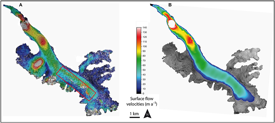
Figure 2. Surface flow velocities for Argentière Glacier derived from SPOT5 images acquired in 2003. (A) Raw data from Berthier et al. (2005). (B) Data after filtering and interpolation.
The raw surface flow velocities derived from Berthier et al. (2005) need to be filtered due to some correlation artifacts that can occur in the part of the glacier where the surface state changes from snow-covered to bare ice between the two images and in the shadowed part (see the red rectangle in Figure 2A). The raw data were filtered as follows: considering a moving window of 25 values (5 × 5) the central value is conserved if: (i) its velocity is less than 800 m yr−1 (this threshold is largely above the maximum values measured in the field, and is only used to remove unrealistic values); (ii) the orientation of the vector does not differ by more than 20° from the orientation of its neighbors; and (iii) the velocity differs by less than 5 m yr−1 from the average of its neighbors. After filtering, the data were interpolated and resampled on a regular 10-m grid using a polynomial function (the degree of the polynomial function can be adapted from one section to the other); the result is shown in Figure 2B.
Glacier Surface Elevation and Outline
We used a digital elevation model (DEM) of the glacier (horizontal resolution of 10 m) generated by photogrammetry on the basis of the aerial photos taken on 20 September 2003, to obtain a temporal overlap with the surface flow velocities computed from the satellite images recorded in 2003. Indeed, because surface flow velocities and thicknesses are related, getting a DEM of the glacier surface topography temporally close to the surface flow velocity measurements is recommended. The acceptable time difference between the two data sources is hard to assess as it will depend on the state of the glacier, i.e., if it is close to steady state or rapidly shrinking/growing.
For agreement with the DEM, we used a glacier outline from 2003, extracted from the multi-temporal inventory of glaciers in the French Alps (Gardent et al., 2014).
Methodology
Description of the Proposed Approach
Our approach requires both the glacier surface flow velocities and the surface mass balances to quantify the ice flux Qj, at the level of cross-section j, perpendicular to the central flow line of the glacier, and to quantify the ice thicknesses along these cross-sections of length lj. The approach can be divided into four main steps:
1. Definition of the cross-sections whose thickness will be computed.
The central flow line of Argentière Glacier was delineated manually from the uppermost elevation to the glacier snout, perpendicular to the contour lines. Next, 59 cross-sections were defined perpendicular to the central flow line (Figure 3), of which 19 are located in the vicinity of the in situ thickness measurements (see Figure 1). The others were defined in between to homogeneously cover the glacier (maximum distance between two cross-sections is 300 m). In the ablation zone, where the glacier tongue is clearly defined (down to cross-section #25 for the two sides of each cross-section, and down to cross-section #44 for the right-hand side only), the limits of the cross-sections are the edges of the glacier. Where tributaries can be found or in the accumulation zone, the cross-sections are delimited using a threshold on the surface flow velocities. The threshold used is a parameter that can be fixed or adjusted from one side to the other of each cross-section and from one cross-section to another when thickness measurements are available in order to optimize the estimated thicknesses. Note that in the present study, we did not define cross-sections on the tributaries because we focused on the main body of Argentière Glacier, where in situ thickness data are available to validate the ice thickness estimates. However, cross-sections can be defined wherever needed.
2. Quantification of the ice flux and the average thickness of each cross-section
Like in Farinotti et al. (2009) and in Huss and Farinotti (2012), the apparent mass balance , was calculated for each grid cell, i, of the glacier surface area. Indeed, for mass conservation in steady-state conditions, the surface mass balance must counterbalance the ice flux divergence. The apparent mass balance profile is computed from the measured surface mass balance profile which is adjusted to get a glacier-wide surface mass balance equal to zero (i.e., steady state condition). Following Farinotti et al. (2009), we assume that the ice flux of each cross-section Qj, is the sum of the apparent mass balances over the total number n of grid cells (with individual surface areas ai), of the portion of the glacier surface contributing to the cross-section j:
On the other hand, the area, Sj, of each cross-section equals the ice flux divided by the average velocity of the cross-section .
According to Cuffey and Paterson (2010, p. 342) matches to within a few percent the mean surface velocity on the profile across the whole glacier, . Nye (1965) showed that the ratio of depends on the ratio W between the half-width (or half-length as denoted here) and depth, and on the value n (n being the power of the stress in the flow law). Assuming a parabolic valley and n = 3, equals 0.837 for W = 1, 0.980 for W = 2, 0.997 for W = 3 and 1.005 for W = 4. According to Cuffey and Paterson (2010), values of W between 2 and 4 include the majority of valley glaciers, therefore we consider 0.99 ± 1%. It is noteworthy that, in the first round of ITMIX, we considered a value of 0.8 (corresponding to no sliding) which was not suited for Argentière Glacier.
Thus, the area of each cross-section can be computed by combining Equations (1) and (2):
From this step, for each cross-section, we obtain an ice flux that satisfies two necessary conditions: (1) the ice flux through the cross-section is equal to the mass balance of the surface area of the glacier contributing to this cross-section; and (2) the average velocity of the ice flowing through a cross-section is within a few percent of the average surface velocity of this cross-section. Since the length lj of the cross-section is known, the average ice thickness for that cross-section can be computed as:
3. Distribution of the thicknesses along the cross-section
Step 3 consists in “distributing” the ice thicknesses along the entire cross-section using the pattern of surface flow velocities. We assume that for each grid cell, i, the ratio between the thickness, hi, and the surface flow velocity, vi, is the same along the whole cross-section, so that hi / vi / , and hence:
It is worth noting that the assumption that hi/vi is the same along the whole cross-section has been tested on cross-sections where both in situ thickness and surface flow velocity measurements are available. Table 1 shows that the overall agreement is good with a coefficient of variation of 10% in average, even if it reaches values close to 40% for the lowermost cross-section, where the valley is highly asymmetric.
4. Extrapolation at the glacier scale
The final step consists of extrapolating the thickness data of each cross-section to the whole glacier. In the current study, this was done using a universal Kriging method with anisotropy in the main glacier flow direction. Indeed, because the glacier valley is assumed to be of U-to-V shape, more weight is given to the neighboring points located along the glacier flow axis vs. points located along the transverse profile. One advantage of Kriging is that inter/extrapolated data do not deviate largely from the initially available values (i.e., on the cross-sections). Some studies have suggested that such interpolation may not conserve mass between the cross-sections (e.g., Morlighem et al., 2011) but that this limitation can be tackled by densifying the number of cross-sections to avoid the need of interpolation (e.g., Seroussi et al., 2011). In the current study, the maximum distance between two cross-sections is 300 m. The distance between cross-sections has been chosen to optimize computation time, but the choice of the number of cross-sections is free, and cross-sections every 10, 50, 100 m, etc. could be considered depending on the resolution of the available data.
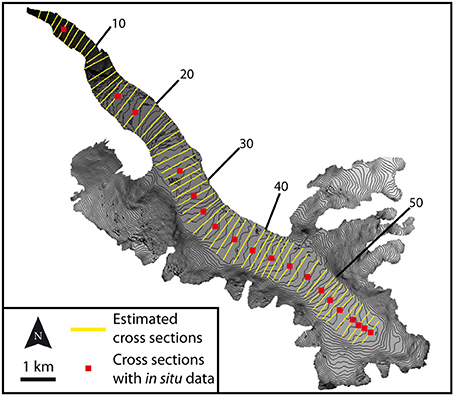
Figure 3. Location of the 59 cross-sections used to estimate the ice thickness on Argentière Glacier. Red squares show the cross-sections for which in situ thickness measurements are available (shown in Figure 1). The cross-sections are numbered up-valley from the snout to the accumulation zone; these numbers indicate the cross sections illustrated in the Results section.
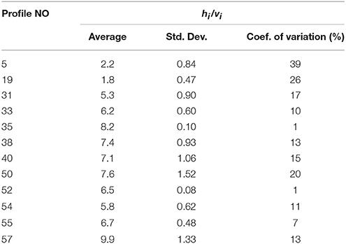
Table 1. Statistics on hi/vi for cross-sections where in situ thickness and surface flow velocity measurements are available.
To summarize, the following data are needed to apply the method:
• a DEM and the outline of the glacier,
• annual surface mass balance data,
• a map of glacier surface flow velocity concomitant to the glacier DEM,
• although it is not a requirement, we recommend in situ thickness measurements for few cross-sections to adjust the mass balance profile and thus the quantification of the ice fluxes.
Quantification of the Uncertainty in the Thickness Estimates
The overall uncertainty in the glacier thickness values, Δhi, can be computed from the uncertainty in each of the variables in Equation 5; i.e., Δvi, , and . This assumes that the variables are independent and non-correlated. Although and are both related to lj, the common variance is limited (r2 = 0.36) for the 59 considered cross-sections due to a large scatter in (ranging from 100 to 400 m) for ranging from 30 to 50 m/yr (this concerns 33 of the 59 cross-sections). Therefore, applying error propagation Δhi can be expressed as:
which can also be expressed as:
where:
• Δvi is 1.7 m yr−1 (see section Surface Flow Velocity Data).
• depends on the uncertainty in Sj and lj (see Equation 4). The uncertainty in lj is negligible when the limits of the cross-sections are the glacier edges (e.g., on the glacier tongue) and depends on the threshold on the surface flow velocities used to delimit the cross sections for the upper reaches of the glacier. In the latter case, we considered that it varies from one cross-section to the other in the order of ±2 pixels. The uncertainty in Sj (Equation 3) depends on the uncertainty in , on and on the uncertainty in the value taken for the ratio (±1%). We assume that the error in ai is negligible. The uncertainty in has been quantified on the basis of the error in the slope of the linear regression between point surface mass balance measurements and elevation.
• The uncertainty in results from the surface velocity at each pixel, i, of the cross-section, j.
Therefore, Δhi varies from one cross-section to another and, for a given cross-section, from one pixel to another. Δhi ranges from ±6 to ±53 m depending on the cross-section and pixel under consideration, with an average value of ±24 m (or a relative uncertainty ranging from ±3 to ±35%, and average value of ±16%).
We remind that, whatever the uncertainty, the accuracy of the approach can only be assessed by comparing the glacier thickness estimates with “true” or reference values which correspond to the in situ thickness measurements. Such a comparison is presented in the Results section below.
Comparison With Farinotti et al. (2009) Approach
The ice thickness estimation method (known as ITEM) has been presented by Farinotti et al. (2009). In ITEM, the thickness is computed at the level of the central flow line of the glacier considering the shear stress (which depends on the surface slope of the glacier) and the ice flux (see Equation 7 in Farinotti et al., 2009). The ice thickness is then extrapolated from the center to the glacier edges (perpendicularly to the central flow line) using an inverse distance averaging function and also considering the local surface slope with a threshold of 5°. These authors performed sensitivity tests and concluded that the sensitivity of their method is higher for the flow rate factor and for the correction factor. Finally, they estimated that individual cross-sectional areas can be reproduced with an accuracy of 20%. Considering the test of sensitivity to the slope we developed in section Sensitivity to the Surface Slope of the present study, this accuracy appears to be optimistic.
ITEM has been further developed by Huss and Farinotti (2012) to include additional physics (e.g., basal sliding, longitudinal variations in the valley shape factor, influence of ice temperature and climatic regime), to be applicable at a global scale. The ice thickness distribution of Argentière Glacier was estimated by these authors, and their results are shown below and compared with the in situ ice thickness measurements made on the glacier. However, because the input data used by Huss and Farinotti (2012) for the glacier thickness estimates are different from the ones used in the current study (e.g., DEM, glacier outline, surface mass balance), their approach (hereafter, H&F approach) has been applied using our input data for a fair comparison of the results. It is worth noting that the glacier surface slope along the central flow line is needed in H&F approach. This slope is computed in two different ways in Farinotti et al. (2009) and Huss and Farinotti (2012): over a varying distance along the flow line and within 10-m elevation range bands, respectively. In the present study, the slope has been quantified at the center of each cross-section (i.e., along the central flow line) considering a distance of 400 m (±200 m upstream and downstream from the cross section), both by averaging the slope of the grid cells over this distance and using the elevation difference and the distance between each extreme; note that the results do not differ depending on the way by which the slope is quantified.
Although the H&F approach and our approach are both based on the mass conservation principle, the steady state assumption and the Glen's flow law, they differ in their formulation and the required input data. For example, the H&F approach requires the glacier surface slope, which is not used in our approach. On the other hand, our approach requires the glacier surface flow velocity, which is not used in H&F approach. In addition, the H&F approach uses several parameters (e.g., a correction factor to account for the contribution of basal sliding to the total flow speed and a flow rate factor; a valley shape factor that can be fine-tuned from one section to another; an ELA estimate to compute the surface mass balance from gradients in the accumulation and ablation zones). One advantage of our approach is that such parameterizations are not required because the valley shape factor, the basal shear stress, the lateral drag (used for example in Li et al. (2012)), as well as other variables such as the ice viscosity, are implicitly taken into account through the use of the profile of glacier surface flow velocities. As a consequence, in our approach only two parameters can be adjusted on the basis on available in situ thickness data: the threshold of the surface flow velocities used to define the limits of the cross-sections (out of the glacier tongue) and the value used to quantify the average flow velocity of the cross-section from the average surface flow velocity.
Results
Quantification of the Ice Fluxes Using the Apparent Mass Balance
In the two approaches applied in the current study, the apparent mass balance (app. MB) needs to be calculated to quantify the ice fluxes. We tested three different MB profiles to quantify the impact on the ice fluxes.
First we used the “Regional MB profile” presented in Farinotti et al. (2009) and Huss and Farinotti (2012). In this case, two surface mass balance gradients for the ablation and the accumulation zones are considered (0.009 and 0.005 m w.e. m−1, respectively). For the accumulation zone, accumulation rates are limited to prevent unrealistically high accumulation, with a maximum accumulation value matching the one found 700 m above the equilibrium-line altitude (ELA). In other words, the accumulation is kept constant for elevations higher than 700 m above the ELA. For Argentière Glacier, the ELA is considered at 2,850 m a.s.l. Note that, with this MB profile, the glacier-wide SMB is 0.15 m w.e.
Second, we used the “GLACIOCLIM MB profile” quantified using Lliboutry (1974) linear approach based on the in situ accumulation and ablation measurements over the 1975–2016 period. The following relationship between the app. MB of each grid cell of the glacier Bi (in m w.e. yr−1) and its elevation zi (in m a.s.l.) is considered: . This linear relationship has a determination coefficient of 0.93. We note that polynomial fits of different degrees were tested (not shown), without improvement in the results. With this linear MB profile, the glacier-wide SMB is −0.5 m w.e.
Third, to obtain the best agreement between the measured and estimated ice fluxes, we quantified an “adjusted GLACIOCLIM MB profile.” With this MB profile, the glacier-wide SMB is 0.20 m w.e. For this adjustment, we only used four of the 19 available cross-sections. Our intention was to keep the remaining cross-sections for validation and also to use a limited number of in situ thickness measurements because, when available, such information is commonly limited to few points/profiles on a glacier. For the adjustment, the surface mass balance was increased above the ELA (enhanced accumulation) and decreased below 2,200 m a.s.l. (enhanced ablation). The need for such an adjustment of the MB profile likely results from the fact that the surface topography of the glacier does not correspond to steady-state, which is a limitation of our approach. This point is discussed in the section Beyond the Steady State Assumption, a Future Line of Research? However, another reason to explain the need for a modification of the accumulation can be that the spatial variability of the accumulation in the upper reaches of the glacier is not fully represented by the available point measurements. As is the case on most of the glaciers monitored worldwide, accumulation measurements are limited in number and commonly taken in accessible and safe areas; for example, areas with avalanche deposits are rarely documented although this accumulation process might be not negligible when the accumulation area is surrounded by high-slope lateral walls.
Figures 4A,B present the three app. MB profiles tested and the comparison between the estimated ice fluxes using these profiles and the one quantified for the 19 cross-sections for which in situ data of glacier thickness and surface velocities are available.
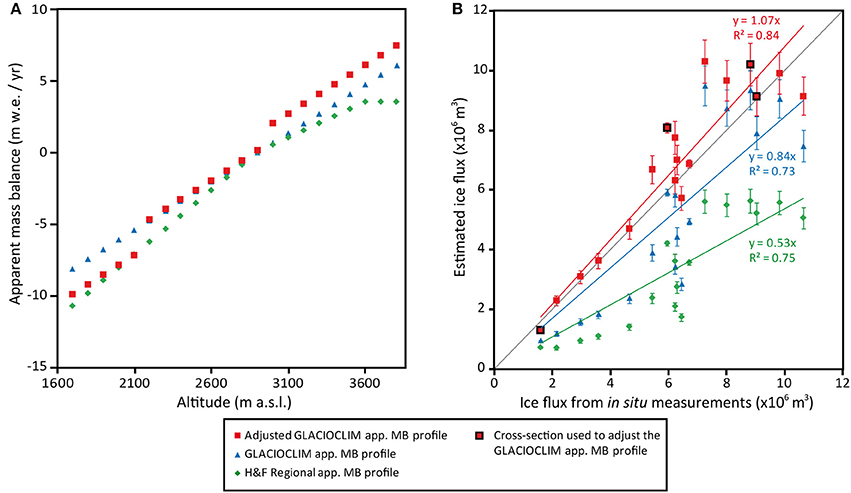
Figure 4. (A) Apparent mass balance profiles (m w.e. yr−1) as a function of altitude (m a.s.l.) used in the present study. (B) Comparison between the ice fluxes quantified from in situ measurements and the ones estimated using the different apparent mass balance profiles for each of the cross sections where glacier thickness was measured. The red squares with a black outline represent the four cross-sections used to adjust the GLACIOCLIM apparent mass balance profile. Uncertainties in the ice fluxes quantified from in situ measurements are too small to be visible on the graph.
For the “Regional app. MB profile” (green diamonds in Figure 4A), Figure 4B shows that such an app. MB profile underestimates the ice fluxes quantified from in situ measurements by about 47%. As a consequence, using a regional relationship between surface mass balance and elevation can lead to significant errors in estimated ice fluxes. It is worth noting that this limitation applies for the results presented in Huss and Farinotti (2012) for Argentière Glacier (see Quantification of the Thicknesses Along the Cross-Sections). In addition, Figure 4A clearly shows that both the app. MB profile and the constant value 700 m above the ELA used in the “Regional app. MB profile” do not present realistic values of accumulation when compared to the GLACIOCLIM MB profile.
Using the “GLACIOCLIM app. MB profile” (blue triangles in Figure 4A), the agreement between the estimated ice fluxes and the ones quantified from in situ measurements is improved in comparison with the “Regional app. MB profile” (underestimation of around 16% instead of 47%). However, Figure 4B shows that using surface mass balance data measured in situ is not completely satisfactory, and results in an overall underestimation of the ice fluxes.
Using the “adjusted GLACIOCLIM app. MB profile” (red squares in Figure 4A), the agreement between the estimated ice fluxes and the ones quantified from in situ measurements is satisfactory (R2 = 0.84), even if it results in a 7% overestimation of the ice fluxes (Figure 4B).
Intermediate conclusions that can be drawn from this first result are: (1) in situ surface mass balance measurements largely improve the estimation of the ice fluxes in comparison with a regional estimate of the mass balance profile, which can lead to large uncertainties; and (2) in situ thickness measurements available for some cross-sections are very useful to better constrain the ice thickness estimations over the entire glacier.
Quantification of the Area of the Cross-Sections
In our approach, the area of each cross-section was assessed from the ice fluxes and using the surface flow velocities obtained from satellite images (Equation 3).
Figure 5 shows the comparison between the estimated areas vs. the areas quantified for each cross section for which in situ thickness measurements are available. The results obtained using different apparent mass balance profiles presented in section Quantification of the Ice Fluxes Using the Apparent Mass Balance are shown to illustrate their influence in the estimation of the area of the cross-section in our approach (Figure 5A) and in the H&F approach (Figure 5B).
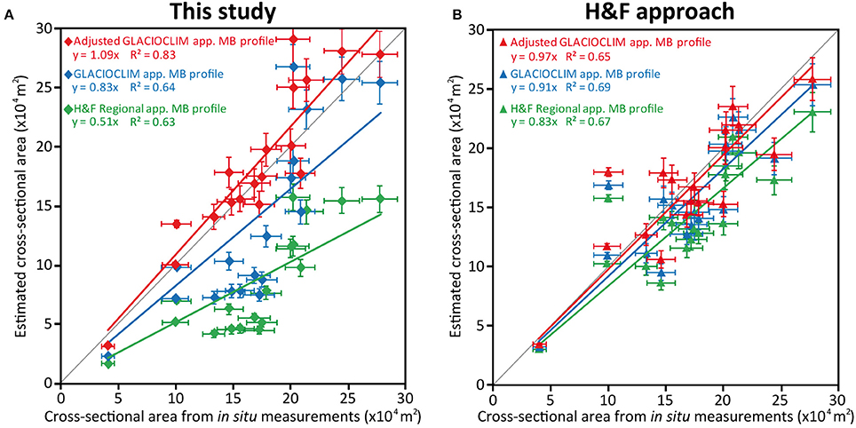
Figure 5. Comparison between the estimated area vs. the measured area for each cross section for which in situ thickness measurements are available. (A) Using our approach. (B) Using Huss and Farinotti (2012) approach.
Using our approach, the area of the cross-section varies considerably depending on the apparent mass balance profile used to quantify the ice flux. With the H&F approach, even with a significant variation in the ice flux (and hence in the apparent mass balance profile used to quantify the ice flux) changes in the cross-sectional area remain limited.
In more detail, the ice flux quantified for the 19 cross-sections illustrated in Figure 4B increases by 55% on average (ranging from 43 to 70% depending on the cross-section concerned) when the “adjusted GLACIOCLIM app. MB profile” is used, in comparison with the “H&F Regional app. MB profile.” Using our approach, this change in the apparent mass balance profile implies a change in the cross-sectional area of 55% while using the H&F approach the change in cross-sectional area is of 15%. This means that in the equation used in the H&F approach to quantify the ice thickness from the ice flux and the shear stress (depending on the surface slope), the importance of the term of the ice flux is limited with regard to the term implying the glacier surface slope. This point will be discussed in more detail in the discussion section.
In the following section, we only present the results obtained using the “adjusted GLACIOCLIM app. MB profile.”
Quantification of the Thicknesses Along the Cross-Sections
In our approach, once the area of the cross-section is estimated, the next step is to quantify the ice thickness along the cross section. This is done using Equation 5.
The results of ice thickness estimations using the “adjusted GLACIOCLIM app. MB profile” are illustrated in Figure 6 for six cross-sections (all the other cross-sections can be found in the Supplementary Material). The average difference and RMSE between estimated and measured ice thicknesses for the 19 cross-sections for which the comparison is possible are −24 m and 78 m with the H&F approach and 4 m and 66 m with our approach. Such average differences and RMSE values are acceptable when considering an uncertainty in seismic or radar thickness measurements of about ±10 m (Vincent et al., 2009).
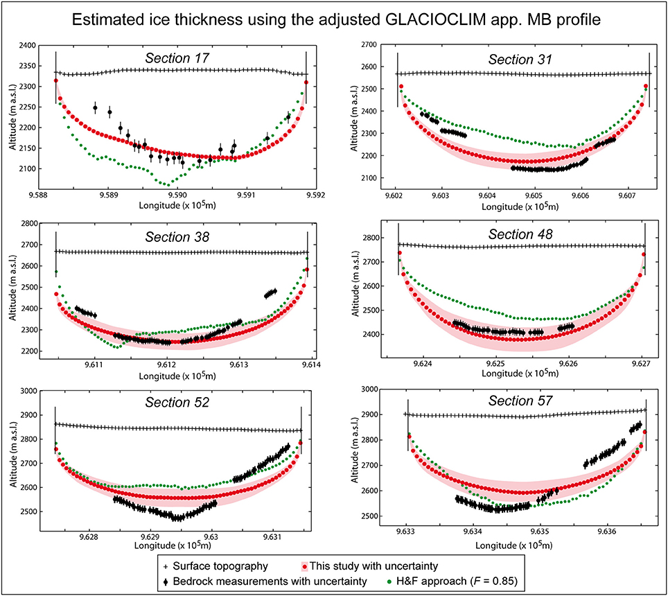
Figure 6. Estimated ice thickness for six cross-sections of Argentière Glacier, using the adjusted GLACIOCLIM apparent mass balance profile. Uncertainties for the H&F approach are not shown for a better legibility (note that these uncertainties are estimated to 20% according to the authors).
Finally, the ice thicknesses estimated for each of the 59 cross-sections with the “adjusted GLACIOCLIM app. MB profile” using the approach presented in the present study and the H&F approach were extrapolated at the glacier scale. Figures 7A,B show the respective maps, together with a map resulting from the extrapolation of the 19 in situ measured cross-sections (Figure 7C) and the original data from Huss and Farinotti (2012) (Figure 7D).
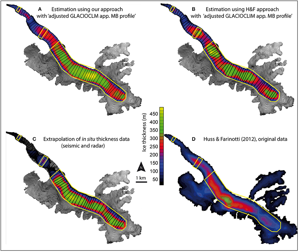
Figure 7. Ice thickness maps of Argentière Glacier using different approaches. (A) The approach used in the present study. (B) The H&F approach. (C) The extrapolated in situ thickness measurements. (D) Original data from Huss and Farinotti (2012). The yellow polygons show the common areas used for comparison of the different data sources.
In terms of ice volume, we considered a common surface area encompassing the available information for the four thickness data sources (Figures 7A–D). This area is of 4.01 km2. Our approach (Figure 7A) gives a total ice volume of 1.216 ± 0.096 × 10⁹ m3. The H&F approach (Figure 7B) gives a total ice volume of 1.069 ± 0.107 × 10⁹ m3. The extrapolation of in situ data (Figure 7C) gives a total ice volume of 1.203 ± 0.06 × 10⁹ m3. The original Huss and Farinotti (2012) dataset (Figure 7D) gives a total ice volume of 0.651 ± 0.065 × 10⁹ m3, which is half the volume given by in situ measurements. The uncertainty in the total volume estimates mainly results from the uncertainties on the approach used to estimate/measure the thickness on the cross-sections. The uncertainty related to the extra/interpolation is comparatively reduced, mainly due to the numerous cross-sections used (e.g., using our approach the average difference between the estimated thickness along the cross-sections before and after interpolation is less than one meter).
The significant underestimation of the volume of the original data provided by Huss and Farinotti (2012) when compared to the in situ thickness measurements cannot be only attributed to the use of an inadequate apparent mass balance profile to quantify the ice fluxes, as we saw that, with their approach, even increasing the ice flux by 55% did not significantly impact the area of the cross-sections. The possible origin of this underestimation is discussed below.
It is worth noting that we focused on the main body of Argentière Glacier where in situ thickness measurements are available for validation of the ice thickness estimates and the adjustment of the MB profile. This does not preclude the application of the method to other areas of glaciers, such as tributaries, as cross-sections can be defined wherever needed.
Discussion
Sensitivity to the Apparent Mass Balance Profile
Figure 8 illustrates the sensitivity of the two methods used in the present study (our approach and the H&F approach) to the mass balance profile used to quantify ice fluxes with the example of the cross-section 48. At this cross-section, using the “adjusted GLACIOCLIM app. MB profile” instead of the “H&F Regional app. MB profile” increases the ice flux by 61%. This difference is logically translated into an increase in the area of the cross-section by the same amount using our approach. In the case of H&F approach, the increase is of only 17%.
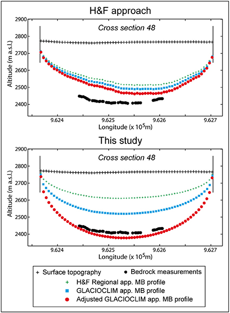
Figure 8. Estimated ice thicknesses (example of cross-section 48) using the different mass balance profiles. Uncertainties are not shown for a better legibility.
Considering the 59 estimated cross-sections, the increase in the ice flux is on average 50% (range: 29–70%) when using the “adjusted GLACIOCLIM app. MB profile” instead of the “H&F Regional app. MB profile.” With the H&F approach, the resulting change in area of the cross-sections is on average 13% (range 11–21%). This shows a limitation of H&F approach.
Sensitivity to the Surface Slope
Because we showed that in the H&F approach, the sensitivity of the thickness to the ice flux is weak, we tested its sensitivity to the surface slope of the glacier.
For a first test we increased the slope threshold used in the H&F approach from 2° to 5°. This resulted in an average decrease in ice thickness of 7% (range: 1–30% depending on the cross-section).
Next, we quantified the slope of the glacier surface at the center of the cross-sections (i.e., along the central flow line) for several distances: 50, 100, 200, and 400 m. As mentioned in section Comparison With Farinotti et al. (2009) Approach, the slope has been quantified along the central flow line considering a distance of 400 m (±200 m upstream and downstream from the cross-section), both by averaging the slope of the grid cells over this distance or using the elevation difference and the distance between each extreme. These two quantifications lead to very similar results and we only show the results obtained when the slope is quantified by averaging the grid cells values.
For the ranges of distance tested, increasing the distance resulted in an increase in the surface slope in 80% of the cases. In addition, the amplitude of the change was positively correlated with the surface slope: the steeper the slope, the larger the amplitude of the change. The average amplitude of the change in slope was 2° (range: 0.2° to 16° depending on the cross-section and distances considered).
In more detail, Table 2 illustrates the impact of the distance over which the glacier surface slope is quantified on the slope and on the thickness at the center of estimated cross-sections using the H&F approach. Figure 9 shows the thickness quantified at the center of different cross-sections with the H&F approach, which graphically illustrates the impact of the distance over which the glacier surface slope is quantified.
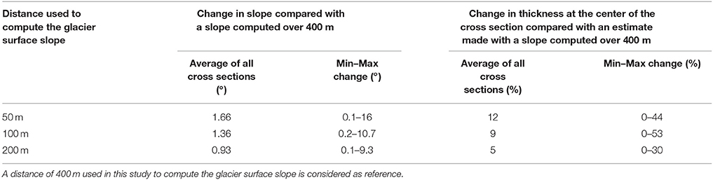
Table 2. Impact of the distance over which the glacier surface slope is quantified on the slope and the thickness at the center of estimated cross-sections using the H&F approach.
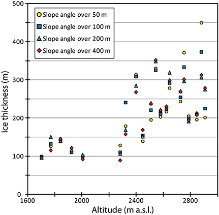
Figure 9. Impact of the distance over which the glacier surface slope is quantified on the thickness at the center of estimated cross-sections using the H&F approach. For better readability, not all the estimated cross-sections are shown in the figure.
From this sensitivity test, it is worth noting that: (1) the glacier surface slope can vary considerably depending on the distance over which it is quantified; and consequently (2) the computed thickness obtained from H&F approach can change by up to 50%. Going into details, in comparison with thickness estimated when the slope is quantified over a distance of 400, the min., average and max. thickness changes are of: 0, 28, and 137 m when the distance used is 50 m; 1, 20, and 83 m when the distance used is 100 m; 0, 10, and 48 m when the distance used is 200 m.
In order to determine the error of the estimated ice thickness due to the slope error εα, in a more general case, we used Equation 7 of Farinotti et al. (2009). The error of ice thickness εhi is expressed as:
This confirms the high sensitivity to the surface slope uncertainty. For instance, considering an ice thickness of 300 m and a surface slope of 3° at the center of a cross-section, an uncertainty in the slope of ±0.5°/1°/1.5°/2° results in an uncertainty in thickness of ±30 m/60 m/90 m/120 m, which is 10%/20%/30%/40% of the thickness considered. This analytical quantification of the uncertainty in the thickness related to the uncertainty in the surface slope is in agreement with the experimental test presented above.
As a consequence, methods that use shear stress to quantify ice thickness, even introducing the quantification of ice fluxes, as is the case in the H&F approach, are highly sensitive to the surface slope of the glacier, which can vary considerably depending on the threshold used and on the distance over which the slope is quantified. Therefore, if such methods are applied, special care must be taken about how the surface slope is calculated, and one must keep in mind that the uncertainty in the estimated ice thickness related to the surface slope is high.
Some Conclusions From the First Round of ITMIX
Farinotti et al. (2017) presented the results of the first round of ITMIX in which our approach was first tested. It is worth reminding that, for this first experiment, no prior knowledge on glacier thickness was available. In addition, our approach was tested on the synthetic case #1 only, so that definitive statements on its performance are hardly feasible.
The synthetic case #1 was the only one for which all participating approaches were tested. Our approach was within the five best solutions in terms of average and median thickness estimates, together with approaches that use an explicit ice flow model (refer to Table S3 in the Supplement of Farinotti et al., 2017). Interestingly, each of these approaches share the use of surface flow velocity as input data. A weakness of our results was an overestimation in the ice thickness, which was mainly attributed to an overestimation of the area contributing to the ice flux of individual cross-sections.
Another interesting result of the experiment on the synthetic case #1 was the ability of approaches using glacier surface flow velocity to faithfully represent the thickness distribution at the glacier scale, whereas approaches based on the shear stress (i.e., using the surface slope) were less prone to do so.
Beyond the Steady State Assumption, a Future Line of Research?
Most of the current approaches used to estimate the glacier thickness (including the present one) are based on the steady state assumption (Farinotti et al., 2017). This hypothesis is conjectural for several reasons:
- The glacier surface topography (hypsometry and surface area) used in the estimation is not representative of a steady state topography.
- The apparent surface mass balance profile computed to obtain a balanced glacier-wide surface mass balance can be quantified in an almost infinite number of ways by varying the accumulation/ablation gradients (equifinality problem). However, this profile determines the ice fluxes and consequently the ice thickness. In the present study, we tested three apparent surface mass balance profiles and showed that the estimated ice fluxes can be strongly affected. Figure 10 shows how the ice fluxes vary for all the estimated cross-sections depending on the apparent surface mass balance profile used, and how the estimated fluxes compare with the measured ones.
- When glacier surface flow velocities are used, these velocities may not be representative of a steady state glacier geometry.
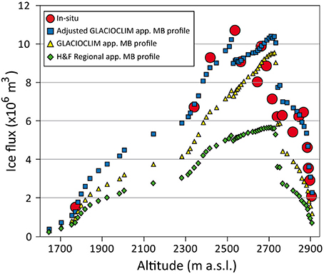
Figure 10. Comparison of ice fluxes for all the estimated cross-sections using different apparent surface mass balance profiles and in situ measurements on Argentière Glacier. Uncertainties are not shown for a better legibility.
As a consequence, the use of the steady state assumption may lead to significant uncertainties in the ice thickness estimates except if, as demonstrated in this study, in situ thickness measurements exist to adjust the surface mass balance profile used to quantify the ice fluxes (or other parameterizations depending on the approach). With the new approach presented here, we have confidence in the estimated ice thicknesses, which differ from observations by only 10% on average.
To avoid using a steady-state assumption, future investigations should take advantages of the recent progress made with 3D full-Stokes ice flow models, and work in a transient mode (e.g., van Pelt et al., 2013). In order to use these methods, the glacier surface elevation, ice flow velocity and surface mass balance need to be known throughout the study period, or at least at the beginning and the end of the period in the case of the surface elevation and velocity. Thanks to the increase in satellite observations (e.g., Gardelle et al., 2013; Berthier et al., 2014, 2016; Dehecq et al., 2016, regarding surface elevation changes and Dehecq et al., 2015; Mouginot and Rignot, 2015; Sánchez-Gámez and Navarro, 2017; Strozzi et al., 2017, regarding ice flow velocity), these latter data are increasingly available, which paves the way for global applications of such an approach.
Conclusions
This paper presents an approach to estimate the glacier thickness distribution on the basis of surface mass balances and surface flow velocities. Although not a requirement in the application of the approach, we also used a few thickness data (in our case, four of the 19 available profiles) to improve the estimated thicknesses. Because such data are not currently available for every glaciers on a global scale, this method does not pretend to be applicable worldwide. However, the increasing number of high spatial resolution satellite data will soon make it possible to have accurate surface flow velocities for every single glacier, including those for which in situ ice thickness data are available (about 2000 glaciers in the Glacier Thickness Database 2.0., WGMS (2016)).
Applying our approach on a well-documented glacier in the French Alps, Argentière Glacier, where in situ measurements of surface mass balances, surface flow velocities and ice thickness are available, we tested the accuracy of the estimated glacier thickness in relation to the input data and showed that:
- the use of a regional surface mass balance profile leads to significant underestimation of the ice fluxes (~50% on average), which has a direct impact on the estimated thicknesses.
- the use of in situ surface mass balance data makes it possible to reduce the uncertainty in the ice fluxes to about 15%.
- the use of in situ thickness measurements (using four of the 19 documented cross sections) made it possible to adjust the surface mass balance profile and to improve the quality of the estimated ice thickness (average difference of 10%).
It is worth noting that because our approach uses surface flow velocities in addition to surface mass balances, the accuracy of the results depends to a great extent on the availability of the surface mass balance data used to quantify the ice fluxes. Indeed, we showed that our approach is very sensitive to the surface mass balance profile used.
We also tested the approach proposed by Farinotti et al. (2009) and Huss and Farinotti (2012). In this approach, the ice flux computed from the surface mass balance is used together with shear stress (depending on the surface slope of the glacier) to quantify ice thickness. We showed that this approach is almost insensitive to surface mass balance but is highly sensitive to the surface slope. Unfortunately, the assessment of surface slope is subject to high uncertainty depending on the distance over which it is quantified. Our error calculation revealed marked uncertainties caused by the uncertainty in the slope, which can reach up to 50% of the calculated thickness. In addition, the use of a threshold on the slope to avoid flat or near-flat surface (which would lead to an infinite thickness when the slope is zero) leads to underestimation of ice thickness for low slope angles. Consequently, methods that use surface slope (e.g., Farinotti et al., 2009; Huss and Farinotti, 2012; Linsbauer et al., 2012; Gantayat et al., 2014) should be used with caution and as minimal estimates with high uncertainty. For instance, we found that the ice volume estimated for Argentière Glacier in Huss and Farinotti (2012) is half the volume quantified from in situ data. Such uncertainties can have a serious impact on estimations of glacier contribution to sea level rise or to the hydrological functioning of glacierized catchments.
Finally, considering the steady state assumption, reasonable estimates of glacier thickness distribution of the entire glacier surface area cannot be obtained without a minimum set of data on surface mass balance, surface flow velocities and a few in situ thickness measurements.
A future line of research could be to estimate ice thickness using an ice flow model in transient mode. To this end, input data such as glacier surface elevation and flow velocity changes over the study period are needed. New satellite products available at global scale open the way for global application of such an approach.
Author Contributions
AR and CV coordinated the study and the writing of the manuscript. OS developed the routines for data processing (satellite-derived velocity filtering, radar data) and thickness estimations. CV, OS, and AR coordinated the radar field campaigns. DS coordinated the surface mass balance measurements within the GLACIOCLIM Observatory. OS and DS revised the manuscript.
Funding
This study was conducted in the context of the VIP_Mont-Blanc project (ANR-14-CE03-0006-03) and in the framework of the Service National d'Observation GLACIOCLIM (http://glacioclim.osug.fr/). This work was made possible thanks to the contributions of: Labex OSUG2020 (Investissements d'avenir - ANR10 LABX56); the CNES/SPOT-Image ISIS SPOT5 images.
Conflict of Interest Statement
The authors declare that the research was conducted in the absence of any commercial or financial relationships that could be construed as a potential conflict of interest.
Acknowledgments
The authors are grateful to Jean-Louis Mugnier, coordinator of the VIP_Mont-Blanc project, to Etienne Berthier for delivering satellite-derived velocities, and to all those who took part in the field measurements, particularly in the radar field campaigns. Finally, we thank F. Navarro (scientific editor) and the two referees R. McNabb and M. Menenti for their constructive comments that helped to improve the paper.
Supplementary Material
The Supplementary Material for this article can be found online at: https://www.frontiersin.org/articles/10.3389/feart.2018.00112/full#supplementary-material
Figure S1. Estimated ice thickness for the cross-sections of Argentière Glacier for which in situ thickness measurements are available (cross-sections #5 to #43, see Figure 3 in the main text to locate the cross-sections on the glacier surface). Estimations were built using the apparent mass balance profile quantified from in situ measurements adjusted using known ice fluxes for four sections. Uncertainties are not shown for a better legibility.
Figure S2. Same as Figure S1 for cross-sections #46 to #59 (see Figure 3 in the main text to locate the cross-sections on the glacier surface). Uncertainties are not shown for a better legibility.
References
Beniston, M., Farinotti, D., Stoffel, M., Andreassen, L. M., Coppola, E., Eckert, N., et al. (2018). The European mountain cryosphere: a review of past, current and future issues. Cryosphere 12, 759–794. doi: 10.5194/tc-12-759-2018
Berthier, E., Cabot, V., Vincent, C., and Six, D. (2016). Decadal region-wide and glacier-wide mass balances derived from multi-temporal ASTER satellite digital elevation models. Validation over the Mont-Blanc area. Front. Earth Sci. 4:63. doi: 10.3389/feart.2016.00063
Berthier, E., Vadon, H., Baratoux, D., Arnaud, Y., Vincent, C., Feigl, K. L., et al. (2005). Surface motion of mountain glaciers derived from satellite optical imagery. Remote Sens. Environ. 95, 14–28. doi: 10.1016/j.rse.2004.11.005
Berthier, E., Vincent, C., Magnússon, E., Gunnlaugsson, Á., Pitte, P., Le Meur, E., et al. (2014). Glacier topography and elevation changes derived from Pléiades sub-meter stereo images. Cryosphere 8, 2275–2291. doi: 10.5194/tc-8-2275-2014
Bindschadler, R. (1982). A numerical model of temperate glacier flow applied to the quiescent phase of a surge-type glacier. J. Glaciol. 28, 239–265. doi: 10.1017/S0022143000011618
Brinkerhoff, D. J., Aschwanden, A., and Truffer, M. (2016). Bayesian inference of subglacial topography using mass conservation. Front. Earth Sci. 4:8. doi: 10.3389/feart.2016.00008
Clarke, G. K. C., Berthier, E., Schoof, C. G., and Jarosch, A. H. (2009). Neural networks applied to estimating subglacial topography and glacier volume. J. Clim. 22, 2146–2160. doi: 10.1175/2008JCLI2572.1
Cuffey, K. M., and Paterson, W. S. B. (2010). The Physics of Glaciers, 4 Edn. Amsterdam: Academic Press Inc.
Dehecq, A., Gourmelen, N., and Trouvé, E. (2015). Deriving large-scale glacier velocities from a complete satellite archive: application to the Pamir–Karakoram–Himalaya. Remote Sens. Environ. 162, 55–66. doi: 10.1016/j.rse.2015.01.031
Dehecq, A., Millan, R., Berthier, E., Gourmelen, N., Trouvé, E., and Vionnet, V. (2016). Elevation changes inferred from TanDEM-X data over the Mont-Blanc area: impact of the X-band interferometric bias. IEEE J. Select. Top. App. Earth Obs. Remote Sens. 9, 3870–3882. doi: 10.1109/JSTARS.2016.2581482
Driedger, C., and Kennard, P. (1986). Glacier volume estimation on Cascade volcanos: an analysis and comparison with other methods. Ann. Glaciol. 8, 59–64. doi: 10.1017/S0260305500001142
Farinotti, D., Brinkerhoff, D., Clarke, G. K. C., Fürst, J. J., Frey, H., Gantayat, P., et al. (2017). How accurate are estimates of glacier ice thickness? Results from itmix, the ice thickness models intercomparison experiment. Cryosphere 11, 949–970. doi: 10.5194/tc-11-949-2017
Farinotti, D., Huss, M., Bauder, A., Funk, M., and Truffer, M. (2009). A method to estimate the ice volume and ice-thickness distribution of alpine glaciers. J. Glaciol. 55, 422–430. doi: 10.3189/002214309788816759
Fischer, A. (2009), Calculation of glacier volume from sparse ice-thickness data, applied to Schaufelferner, Austria. J. Glaciol. 55, 453–460. doi: 10.3189/002214309788816740.
Fürst, J. J., Gillet-Chaulet, F., Benham, T. J., Dowdeswell, J. A., Grabiec, M., Navarro, F., et al. (2017). Application of a two-step approach for mapping ice thickness to various glacier types on Svalbard. Cryosphere 11, 2003–2032. doi: 10.5194/tc-11-2003-2017
Gantayat, P., Kulkarni, A. V., and Srinivasan, J. (2014). Estimation of ice thickness using surface velocities and slope: case study at Gangotri Glacier, India. J. Glaciol. 60, 277–282. doi: 10.3189/2014JoG13J078
Gardelle, J., Berthier, E., Arnaud, Y., and Kaab, A. (2013). Region-wide glacier mass balances over the Pamir-Karakoram-Himalaya during 1999-2011. Cryosphere 7, 1885–1886. doi: 10.5194/tc-7-1885-2013
Gardent, M., Rabatel, A., Dedieu, J.-P., and Deline, P. (2014). Multitemporal glacier inventory of the French Alps from the late 1960s to the late 2000s. Glob. Planet. Chang. 120, 24–37. doi: 10.1016/j.gloplacha.2014.05.004
GLIMS (2013). GLIMS Glacier Inventory, eds R. Armstrong, B. Raup, S. J. S. Khalsa, R. Barry, J. Kargel, C. Helm, and H. Kieffer (Boulder, CO: National Snow and Ice Data Center). Digital media Available online at: http://www.glims.org
Gudmundsson, G. H. (1999). A three-dimensional numerical model of the confluence area of Unteraargletscher, Bernese Alps, Switzerland. J. Glaciol. 45, 219–230. doi: 10.1017/S0022143000001726
Haeberli, W., and Hoelzle, M. (1995). Application of inventory data for estimating characteristics of and regional climate-change effects on mountain glaciers: a pilot study with the European Alps. Ann. Glaciol. 21, 206–212. doi: 10.1017/S0260305500015834
Hantz, D. (1981). Dynamique et Hydrologie du Glacier d'Argentière. Ph.D. thesis, Université de Grenoble, Grenoble.
Hubbard, A., Blatter, H., Nienow, P., Mair, D., and Hubbard, B. (1998). Comparison of a three dimensional model flow with field data from Haut Glacier d'Arolla, Switzerland. J. Glaciol. 44, 368–378.
Huss, M., and Farinotti, D. (2012). Distributed ice thickness and volume of all glaciers around the globe. J. Geophys. Res. 117:F04010. doi: 10.1029/2012JF002523
Huss, M., Farinotti, D., Bauder, A., and Funk, M. (2008). Modelling runoff from highly glacierized alpine drainage basins in a changing climate. Hydrol. Process. 22, 3888–3902. doi: 10.1002/hyp.7055
Huss, M., Jouvet, G., Farinotti, D., and Bauder, A. (2010). Future high-mountain hydrology: a new parameterization of glacier retreat. Hydrol. Earth Syst. Sci. 14, 815–829. doi: 10.5194/hess-14-815-2010
Jouvet, G., Huss, M., Funk, M., and Blatter, H. (2011). Modelling the retreat of Grosser Aletschgletscher, Switzerland, in a changing climate. J. Glaciol. 57, 1033–1045. doi: 10.3189/002214311798843359
Le Meur, E., and Vincent, C. (2003). A two-dimensional shallow ice flow of glacier de saint sorlin, France. J. Glaciol. 49, 527–538. doi: 10.3189/172756503781830421
Li, H., Ng, F., Li, Z., Qin, D., and Cheng, G. (2012). An extended “perfect plasticity” method for estimating ice thickness along the flow line of mountain glaciers. J. Geophys. Res. 117:F01020. doi: 10.1029/2011JF002104
Linsbauer, A., Paul, F., and Haeberli, W. (2012). Modeling glacier thickness distribution and bed topography over entire mountain ranges with GlabTop: application of a fast and robust approach. J. Geophys. Res. 117:F03007. doi: 10.1029/2011JF002313
Linsbauer, A., Paul, F., Machguth, H., and Haeberli, W. (2013). Comparing three different methods to model scenarios of future glacier change in the Swiss Alps. Ann. Glaciol. 54, 241–253. doi: 10.3189/2013AoG63A400
Lliboutry, L. (1974). Multivariate statistical analysis of glacier annual balances. J. Glaciol. 13, 371–392.
McNabb, R. W., Hock, R., O'Neel, S., Rasmussen, L. A., Ahn, Y., Braun, M., et al. (2012). Using surface velocities to calculate ice thickness and bed topography: a case study at Columbia Glacier, Alaska, USA. J. Glaciol. 58, 1151–1164. doi: 10.3189/2012JoG11J249
Mingo, L., and Flowers, G. E. (2010). An integrated lightweight ice penetrating radar system. J. Glaciol. 56, 709–714. doi: 10.3189/002214310793146179
Morlighem, M., Rignot, E., Seroussi, H., Larour, E., Ben Dhia, H., and Aubry, D. (2011). A mass conservation approach for mapping glacier ice thickness. Geophys. Res. Lett. 38. doi: 10.1029/2011GL048659
Mouginot, J., and Rignot, E. (2015). Ice motion of the Patagonian icefields of South America: 1984–2014. Geophy. Res. Lett. 42, 1441–1449. doi: 10.1002/2014GL062661
Nye, J. F. (1965). The flow of a glacier in a channel of rectangular, elliptic or parabolic cross-section. J. Glaciol. 5, 661–690. doi: 10.1017/S0022143000018670
Oerlemans, J., Anderson, B., Hubbard, A., Huybrechts, P., Johannesson, T., Knap, W. H., et al. (1998). Modelling the response of glaciers to climate warming. Climate Dyn. 14, 267–274. doi: 10.1007/s003820050222
Pfeffer, W. T., Arendt, A., Bliss, A., Bolch, T., Cogley, J. G., Gardner, A., et al. (2014). The randolph glacier inventory: a globally complete inventory of glaciers. J. Glaciol. 60, 537–552. doi: 10.3189/2014JoG13J176
Rabatel, A., Dedieu, J.-P., and Vincent, C. (2016). Spatio-temporal changes in glacier-wide mass balance quantified by optical remote-sensing on 30 glaciers in the French Alps for the period 1983-2014. J. Glaciol. 62, 1153–1166. doi: 10.1017/jog.2016.113
Rabatel, A., Letréguilly, A., Dedieu, J.-P., and Eckert, N. (2013). Changes in glacier equilibrium-line altitude in the western Alps from 1984 to 2010: evaluation by remote sensing and modeling of the morpho-topographic and climate controls. Cryosphere 7, 1455–1471. doi: 10.5194/tc-7-1455-2013
Réveillet, M., Rabatel, A., Gillet-Chaulet, F., and Soruco, A. (2015). Simulations of changes in Glaciar Zongo, Bolivia (16°S), over the 21st century using a 3D full-Stokes model and CMIP5 climate projections. Ann. Glaciol. 56, 89–97. doi: 10.3189/2015AoG70A113
Reynaud, M. (1959). Prospection au Glacier d'Argentière. Paris: Société Hydrotechnique de France, Section Glaciologie.
Sánchez-Gámez, P., and Navarro, F. J. (2017). Glacier surface velocity retrieval using D-InSAR and offset tracking techniques applied to ascending and descending passes of Sentinel-1 data for Southern Ellesmere ice caps, Canadian Arctic. Remote Sens. 9:442. doi: 10.3390/rs9050442
Seroussi, H., Morlighem, M., Rignot, E., Larour, E., Aubry, D., Ben Dhia, H., et al. (2011). Ice flux divergence anomalies on 79north Glacier, Greenland. Geophys. Res. Lett. 38:L09501. doi: 10.1029/2011GL047338
Strozzi, T., Paul, F., Wiesmann, A., Schellenberger, T., and Kääb, A. (2017). Circum-Arctic changes in the flow of glaciers and ice caps from satellite SAR data between the 1990s and 2017. Remote Sens. 9:947. doi: 10.3390/rs9090947
Sugiyama, S., Bauder, A., Conradin, Z., and Funk, M. (2007). Evolution of rhonegletscher, Switzerland, over the past 125 years and in the future: application of an improved flow line model. Ann. Glaciol. 46, 268–274. doi: 10.3189/172756407782871143
van Pelt, W. J. J., Oerlemans, J., Reijmer, C. H., Pettersson, R., Pohjola, V. A., Isaksson, E., et al. (2013). An iterative inverse method to estimate basal topography and initialize ice flow models. Cryosphere 7, 987–1006. doi: 10.5194/tc-7-987-2013
Vincent, C., Harter, M., Gilbert, A., Berthier, E., and Six, D. (2014). Future fluctuations of Mer de Glace, French Alps, assessed using a parameterized model calibrated with past thickness changes. Ann. Glaciol. 55, 15–24. doi: 10.3189/2014AoG66A050
Vincent, C., Soruco, A., Six, D., and Le Meur, E. (2009). Glacier thickening and decay analysis from 50 years of glaciological observations performed on Glacier d'Argentière, Mont-Blanc area, France. Ann. Glaciol. 50, 73–79. doi: 10.3189/172756409787769500
Vuille, M., Huggel, C., Carey, M., Buytaert, W., Rabatel, A., Jacobsen, D., et al. (2018). Rapid decline of snow and ice in the tropical Andes - Impacts, uncertainties and challenges ahead. Earth-Sci. Rev. 176, 195–213. doi: 10.1016/j.earscirev.2017.09.019
WGMS (2016). Glacier Thickness Database 2.0, eds I. Gärtner-Roer, L. M. Andreassen, E. Bjerre, D. Farinotti, A. Fischer, M. Fischer, et al. Zurich: World Glacier Monitoring Service. Available online at: https://www.gtn-g.ch/data_catalogue_glathida/
Keywords: glacier thickness, glacier surface mass balance, glacier surface flow velocity, satellite remote sensing, French Alps
Citation: Rabatel A, Sanchez O, Vincent C and Six D (2018) Estimation of Glacier Thickness From Surface Mass Balance and Ice Flow Velocities: A Case Study on Argentière Glacier, France. Front. Earth Sci. 6:112. doi: 10.3389/feart.2018.00112
Received: 20 February 2018; Accepted: 23 July 2018;
Published: 14 August 2018.
Edited by:
Francisco José Navarro, Universidad Politécnica de Madrid (UPM), SpainReviewed by:
Massimo Menenti, Delft University of Technology, NetherlandsRobert McNabb, University of Oslo, Norway
Copyright © 2018 Rabatel, Sanchez, Vincent and Six. This is an open-access article distributed under the terms of the Creative Commons Attribution License (CC BY). The use, distribution or reproduction in other forums is permitted, provided the original author(s) and the copyright owner(s) are credited and that the original publication in this journal is cited, in accordance with accepted academic practice. No use, distribution or reproduction is permitted which does not comply with these terms.
*Correspondence: Antoine Rabatel, antoine.rabatel@univ-grenoble-alpes.fr