Article

On the Importance of High-Resolution Time Series of Optical Imagery for Quantifying the Effects of Snow Cover Duration on Alpine Plant Habitat

by
Jean-Pierre Dedieu
1,2,3,*,†,
Bradley Z. Carlson
4,5,6,†,
Sylvain Bigot
1,2,3,6,
Pascal Sirguey
7,
Vincent Vionnet
8,9 and
Philippe Choler
4,5,6,10
1
Laboratoire d’étude des Transferts en Hydrologie et Environnement, Université Grenoble Alpes, 460 rue de la Piscine, Saint Martin d’Hères 38400, France
2
Institut de Recherche pour le Développement, Laboratoire d’étude des Transferts en Hydrologie et Environnement, 460 rue de la Piscine, Saint Martin d’Hères 38400, France
3
Centre National de la Recherche Scientifique, Laboratoire d’étude des Transferts en Hydrologie et Environnement, 460 rue de la Piscine, Saint Martin d’Hères 38400, France
4
Université Grenoble Alpes, Laboratoire d’Ecologie Alpine, 2233 rue de la Piscine, Saint Martin d’Hères 38400, France
5
Centre National de la Recherche Scientifique, Laboratoire d’Ecologie Alpine, 2233 rue de la Piscine, Saint Martin d’Hères 38400, France
6
Long Term Ecological Research Network “Zone Atelier Alpes”, Saint Martin d’Hères 38400, France
7
University of Otago, National School of Surveying, P.O. Box 56, Dunedin 9054, New Zealand
8
Météo-France, Centre d’Etudes de la Neige, 1441 rue de la Piscine, Saint Martin d’Hères 38400, France
9
Centre National de la Recherche Scientifique, Centre d’Etudes de la Neige, 1441 rue de la Piscine, Saint Martin d’Hères 38400, France
10
Centre National de la Recherche Scientifique, Station Alpine Joseph Fourier, 2233 rue de la Piscine, Saint Martin d’Hères 38400, France
*
Author to whom correspondence should be addressed.
These authors contributed equally to this work.
Remote Sens. 2016, 8(6), 481; https://doi.org/10.3390/rs8060481
Submission received: 11 March 2016 / Revised: 13 May 2016 / Accepted: 2 June 2016 / Published: 7 June 2016

Abstract

:
We investigated snow cover dynamics using time series of moderate (MODIS) to high (SPOT-4/5, Landsat-8) spatial resolution satellite imagery in a 3700 km2 region of the southwestern French Alps. Our study was carried out in the context of the SPOT (Take 5) Experiment initiated by the Centre National d’Etudes Spatiales (CNES), with the aim of exploring the utility of high spatial and temporal resolution multispectral satellite imagery for snow cover mapping and applications in alpine ecology. Our three objectives were: (i) to validate remote sensing observations of first snow free day derived from the Normalized Difference Snow Index (NDSI) relative to ground-based measurements; (ii) to generate regional-scale maps of first snow free day and peak standing biomass derived from the Normalized Difference Vegetation Index (NDVI); and (iii) to examine the usefulness of these maps for habitat mapping of herbaceous vegetation communities above the tree line. Imagery showed strong agreement with ground-based measurements of snow melt-out date, although R2 was higher for SPOT and Landsat time series (0.92) than for MODIS (0.79). Uncertainty surrounding estimates of first snow free day was lower in the case of MODIS, however (±3 days as compared to ±9 days for SPOT and Landsat), emphasizing the importance of high temporal as well as high spatial resolution for capturing local differences in snow cover duration. The main floristic differences between plant communities were clearly visible in a two-dimensional habitat template defined by the first snow free day and NDVI at peak standing biomass, and these differences were accentuated when axes were derived from high spatial resolution imagery. Our work demonstrates the enhanced potential of high spatial and temporal resolution multispectral imagery for quantifying snow cover duration and plant phenology in temperate mountain regions, and opens new avenues to examine to what extent plant community diversity and functioning are controlled by snow cover duration.

Graphical Abstract

1. Introduction

1.1. Background and Rationale

Mountain regions are privileged areas for water and energy exchanges. Mountain rivers provide water supply to 40% of the world’s population and are subject to high demographic and climate pressure [1]. In many mountain watersheds, the seasonal evolution of the snow pack is a key parameter influencing regional climate [2], water resource budgets [3], and ecosystem functioning and structure [4]. Within the context of global climate change [1,5], temperature rise in the European Alps has been pronounced and accompanied by rising snow lines and earlier melt-out dates [6,7]. Recent studies show that a continuous winter snow pack is becoming increasingly rare in Alpine catchments below 1200 m above sea level (a.s.l.) [8], although snow cover duration above 2000 m a.s.l. has been shown to be less sensitive to changes in air temperature [9]. Over the last few decades, observational studies of mountain vegetation have demonstrated rising tree lines in the Alps and Pyrenees in response to climate warming and land abandonment [10,11] as well as increasing species richness on Europe’s temperate alpine summits [12].
Optical remote sensing provides the opportunity to address the question of snow cover regime changes at the regional scale, particularly in the context of mid-latitude study areas [13]. A decrease in snow-covered areas has been globally observed in the Northern Hemisphere since the end of the 1970s, when the first space borne optical sensors began to monitor the Earth’s surface [14,15]. Different methods have been developed to compute changes in terms of snow cover area (SCA) and snow cover duration (SCD) [16,17], and have been applied (i) at the global scale with NOAA-AVHRR, SPOT-Vegetation and MODIS sensors; and (ii) at the regional scale with Landsat, SPOT and ASTER missions. The main parameters analyzed are the timing and duration of the melting season under current and future climate conditions [18,19]. Maps and statistics retrieved [13,20] are useful for a large panel of climate and environmental applications, including alpine ecology. Alpine ecologists are especially interested in snow cover maps in order to better understand and predict responses of high-elevation vegetation to climate change [21].
Temperate mountain grasslands are fundamentally limited by a short growing season, and spatial variability in energy availability is a key factor affecting the distribution of high-elevation plant species [22]. Growing season length, as determined by snow cover duration, has been associated with (i) patterns of taxonomic and functional diversity in alpine plant communities [23,24] as well as diversity patterns across plant and microbe trophic levels [25]; and (ii) ecosystem functioning, including primary productivity and phenology [26,27], and nutrient cycling [28]. Turnover in alpine plant diversity typically occurs over short distances (<50 m) in the form of complex mosaics that vary according to topographic heterogeneity [29], which necessitates quantifying changes in environmental conditions at this scale [30]. For plant ecologists interested in understanding and predicting responses of alpine plant communities to climate change, there is therefore a crucial need to map snow cover dynamics at high resolution and over broad spatial scales, both for the present and coming decades [31].
Prior to application of remote sensing-derived snow cover information, it is necessary to carry out ground validation and also to assess cross-scalar agreement between field measurements and imagery of varying spatial and temporal resolutions. Using MODIS imagery at the regional scale, strong agreement was demonstrated between snow maps derived from the Normalized Difference Snow Index (NDSI) and ground-based measurements of snow height [32]. Also using MODIS, phenology metrics for above-tree line vegetation, including snow melt-out date, start of plant growth, and end of the growing season derived from the Normalized Difference Vegetation Index (NDVI) were validated with respect to ground measures of snow and plant height [33]. While at least one previous study has carried out quantitative comparison of snow cover area maps generated by Landsat ETM+ and MODIS satellites [34], studies testing the ability of dense time series of optical imagery at high spatial resolution (<30 m) to quantify snow cover duration in mountainous areas are lacking, and are necessary as the availability of high-resolution satellite imagery continues to increase.
A new technical step is in reach with the Sentinel-2 Copernicus program, including two optical platforms (2A launched successfully in June 2015 and 2B planned for 2016) with high temporal (5 days) and spatial (10 to 20 m) resolutions for coverage of 300 × 300 km2. These combined advantages offer to reduce data gaps caused by cloud cover, and, concerning snow, to improve accuracy for monitoring the timing of snow accumulation and snow melt-out relative to the larger repeat cycles of Landsat or SPOT missions. In order to simulate the Sentinel-2 revisit frequency and output products, the French Space Agency CNES (Centre National d’Etudes Spatiales), joined by the European Space Agency (ESA), implemented the SPOT (Take 5) Experiment, which consisted of moving the SPOT-4 and SPOT-5 satellites to a lower orbit before the end of their respective missions, in order to achieve five-day revisit capacity [35]. The two experiments took place respectively from February to June, 2013, for SPOT-4 (20 m resolution), and from April to September 2015, for SPOT-5 (10 m resolution) over worldwide selected sites, including our study area in the southwestern French Alps.

1.2. Goals and Objectives

Using images obtained from the SPOT (Take 5) Experiment, the objectives of this paper are: (i) to validate remote sensing observations of first snow free day derived from the Normalized Difference Snow Index relative to ground-based measurements for two snowmelt cycles (2013 and 2015); (ii) to generate regional-scale maps of first snow free day and peak productivity defined by the Normalized Difference Vegetation Index; and (iii) to examine the usefulness of these maps for habitat mapping of herbaceous vegetation communities above the tree line. The description of our study area, data sets and climate context are presented in Section 2. Section 3 provides methods for image processing, snow cover (NDSI) and NDVI mapping, validation of snow cover maps and intersection of remote sensing data with vegetation plots. Results are shown in Section 4 for validation of remote sensing estimates of snow melt-out date, regional-scale mapping of first snow free day and peak NDVI, and differentiation of alpine plant community habitat. These findings are discussed in Section 5, followed by our conclusions.

2. Study Area and Data Sets
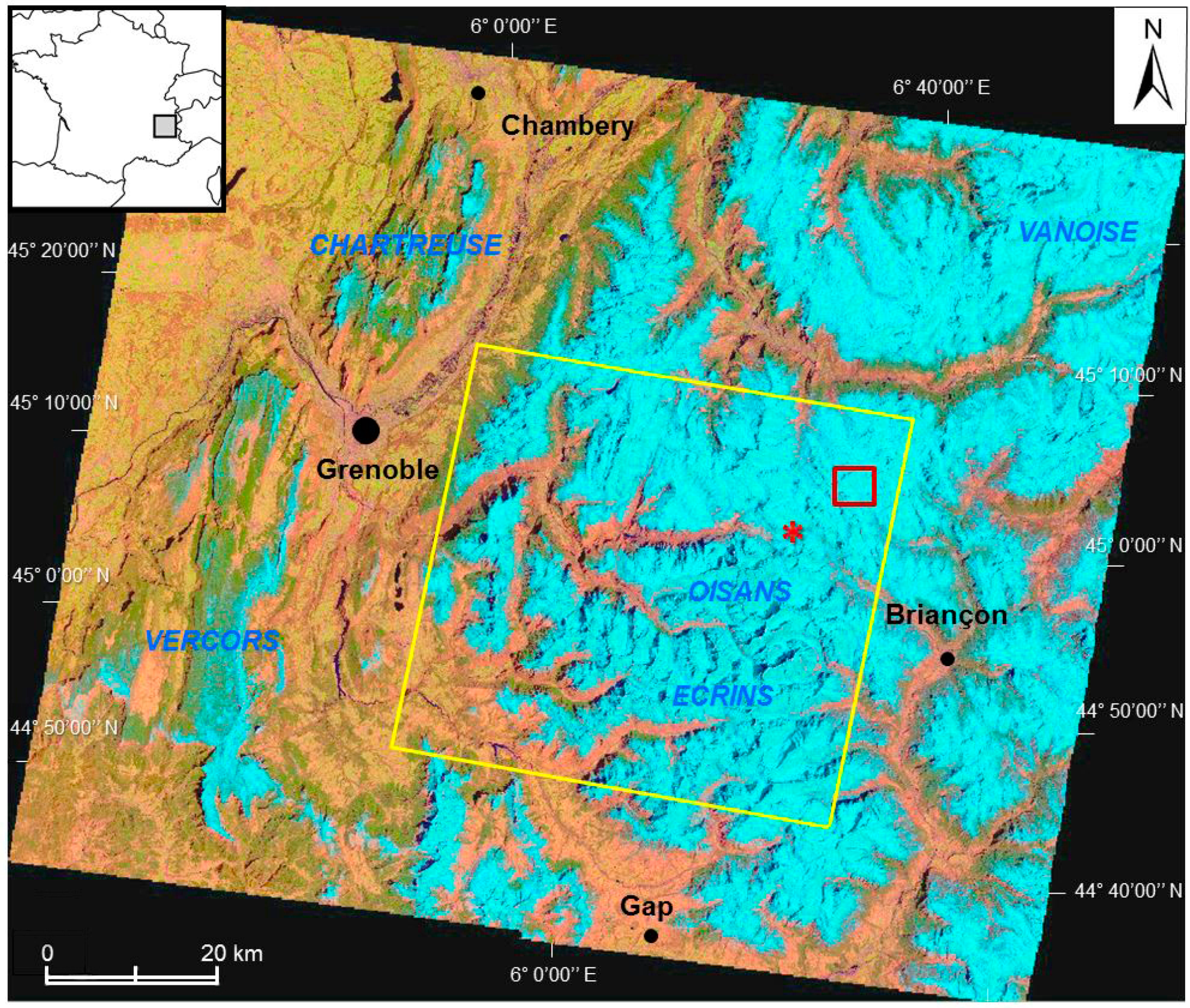
2.1. Study Area

The SPOT (Take 5) study site (French Alps, Europe) is located at 45°09′N, 06°10′E, near the city of Grenoble. It is a high mountain area, centered on the Oisans massif, where 50% of the territory is located at an elevation of over 2000 m a.s.l., including both ski resorts and glaciers (Figure 1). Land cover above inhabited valleys is a combination of forest (mainly spruce, beech, larch and fir) interspersed with grasslands and subalpine heathlands, transitioning to alpine meadows (Figure 2), and finally rock, snowfield and glacier at the highest elevations. Our study area encompasses the Oisans mountain range in the Ecrins National Park, which is a long-term study site for both Météo France and the Long Term Ecological Research Network (LTER) “Zone Atelier Alpes” [36].

2.2. Remote Sensing Data

The SPOT (Take 5) Experiment was carried out using SPOT-4 and 5 satellites. By combining both SPOT-4 sensors, it was possible to obtain an image tile of 110 × 110 km2, whereas the SPOT-5 images were registered under the regular size of 65 × 65 km2, using only a single sensor (Figure 1). The dataset was completed with Landsat-8 acquisitions available beginning in April 2013, and with near-daily MODIS images (L1B swath data product). The complete image collection was cropped to the SPOT-5 extent, in order to be consistent for image pre-processing, mapping and analysis. We used a digital elevation model (DEM) at 25 m resolution and a forest layer provided by the French National Institute Geographic Information (IGN) to remove pixels from the analysis that were forested and or below 1800 m a.s.l. We selected the threshold of 1800 m a.s.l. in order to focus our study on snow cover dynamics and high-elevation plant communities above the tree line.
With spectral bands in the visible and infrared, the optical sensors of SPOT, Landsat and MODIS are appropriate to differentiate snow cover from other targets, particularly above the tree line, including vegetation, bare ground, water and clouds. The physical properties of snow retrieved by optical remote sensing are well documented, especially for energy balance or runoff modeling [37,38,39]. However, additional pre-processing steps are necessary in order to generate usable time series from multiple optical sensors, especially in the case of mountainous study areas [40].

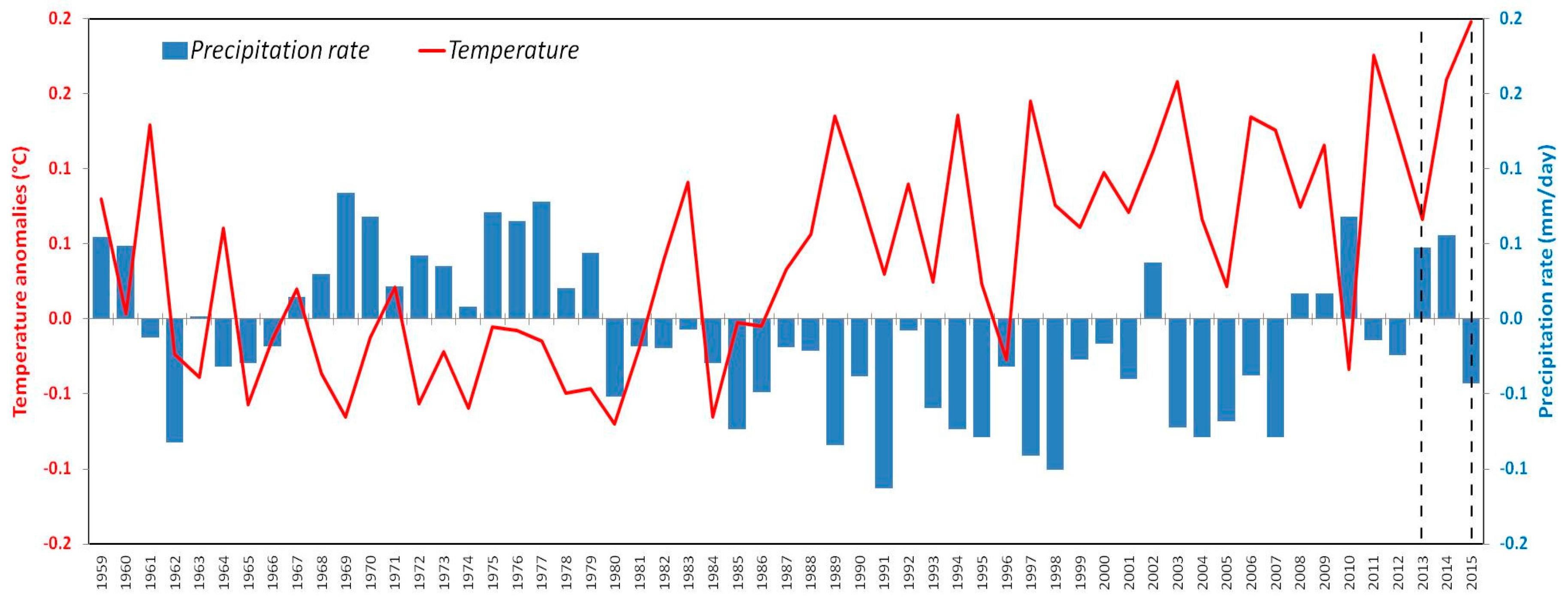
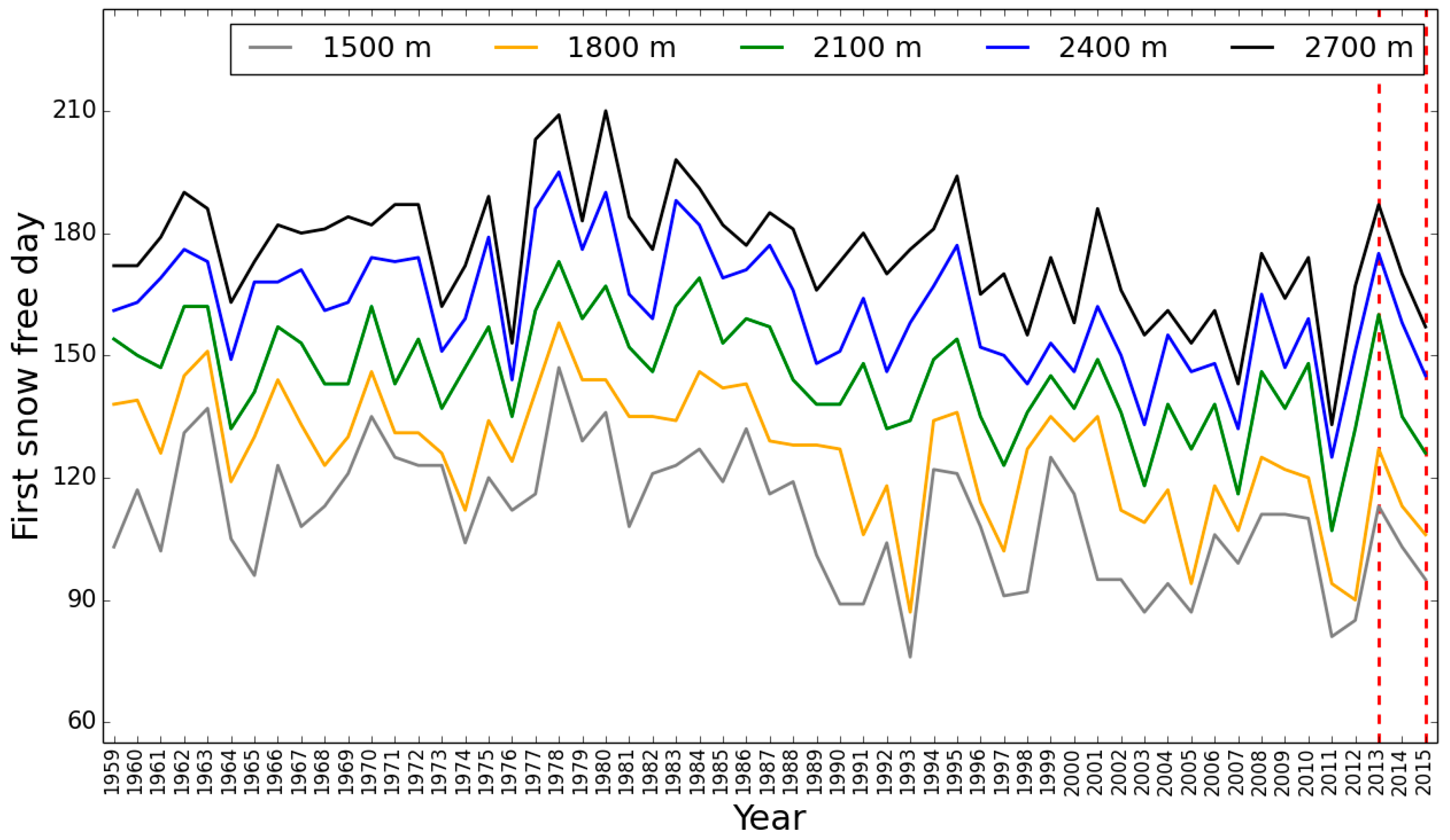
2.3. Climate Context and Snow Cover Variability (1959–2015)

We provide re-analysis of climate and snow cover trends during the past six decades in order to put our study years (2013 and 2015) in context. Recent climate trends in the Europeans Alps have had a strong impact on snow cover duration and environmental conditions for alpine plants [41]. Durand et al. [42] demonstrated a decline in snow cover duration in the French Alps between 1959 and 2005, particularly at low and medium elevations, caused by increases in air temperature coupled with changes in precipitation regimes [43,44,45]. With an increase in annual mean temperatures of 0.9 °C, as compared to a global averaged increase of 0.6 ± 0.2 °C [1], the European Alps have been strongly affected by recent climate change (Figure 3). Within the context of our study area, Figure 4 demonstrates inter-annual variability of the first snow free day for five elevation classes in the Oisans mountain range from August 1958 to August 2015. These results were obtained from a re-analysis of meteorological and snowpack conditions using the SAFRAN-SURFEX/Crocus-MEPRA model chain (S2M) [42,44,46]. At all elevations, snow melt-out date tends to occur earlier in the season during recent years as compared to past decades, although there is substantial year-to-year variability. At 1500 m a.s.l., the first snow free day occurred on average by Julian Day 119 for the period 1961–1990 and by Julian Day 106 over the period 1981–2010 (Figure 4). This trend was less pronounced at 2700 m a.s.l., where first snow free day advanced from Julian Day 182 to 172 between the 1961–1990 and 1981–2010 periods.
The years 2013 and 2015 were highly distinct compared to recent years in our study area in terms of precipitation, temperature and snow cover duration (Figure 3 and Figure 4). Across all elevations, and as compared to average first snow free day values for 1981–2010, 2013 was characterized by exceptionally long-lasting snow cover, whereas snow melt-out occurred relatively early during the spring and early summer of 2015. Substantial climatic differences between study years 2013 and 2015 allowed us to validate our method of estimating the first snow free day for two highly contrasting snowmelt cycles.

3. Materials and Methods

3.1. Image Processing and Snow Cover Mapping

3.1.1. SPOT-4 and SPOT-5 and Landsat-8 Image Pre-Processing

In the framework of the SPOT (Take 5) Experiment, CNES-Cesbio provided SPOT-4 and SPOT-5 images at the top of the atmosphere (L1C) and top of the canopy (L2A) reflectance using the multi-sensor atmospheric correction and cloud screening (MACCS) algorithm [47]. The standard L2A product with “surface reflectance” (hereafter referred to as L2A-SRE) was further enhanced by applying correction methods originally proposed by Dymond and Sheperd [48,49] to account for changes in illumination caused by slope angle and aspect, with the aim of providing a retrieved “flat reflectance” (hereafter referred to as L2A-FRE). Given that designated sites for the SPOT (Take 5) Experiment occurred across the globe, the Shuttle Radar Topography Mission (SRTM) 90 m product was used as the DEM for image processing. All processed SPOT (Take 5) images may be freely downloaded from the CNES-ESA web portal (https://spot-take5.org). To complete the time series for 2013 and 2015, we added available Landsat-8 images at 30 m resolution for both years, which were processed by the THEIA Land Data Center using the same atmosphere and slope-correction algorithms as for SPOT (Take 5) outputs. These data are also distributed with a free and open policy (https://theia-land.fr). Considering the L2A-FRE output as the optimal available product, particularly for early spring months characterized by low solar elevation, we acquired all SPOT and Landsat images for this study at this enhanced correction level. In total, we used thirty-eight high-resolution images (see Table S1 in Supplementary Material), including six SPOT-4 dates (2013), eleven SPOT-5 dates (2015), and twenty-one Landsat-8 dates (nine for 2013, twelve for 2015). SPOT and Landsat images with contrasting spatial resolutions (10–30 m, Table S1) were resampled to a baseline 25 m resolution using bilinear interpolation.

3.1.2. MODIS Image Processing

From February 2000 onward, the MODIS sensor onboard the Terra platform has acquired images worldwide with daily temporal resolution. The National Snow and Ice data Center (NSIDC) provides snow map products at daily and eight-day intervals [50,51]. However, the steep topography of our study area necessitated the use of an enhanced algorithm for detecting snow cover in mountainous terrain using MODIS data. MODImLab is a MATLAB toolbox allowing MODIS L1B swath data products (radiance at the top of atmosphere TOA) to be downloaded and processed automatically towards the production of binary snow maps and maps of sub-pixel snow fraction [52] snow albedo [53], and snow specific surface area [54]. In this study, MODImLab was used to process MODIS/TERRA L1B data using the image fusion approach, which allows for estimation of the short wave infrared band at 250 m spatial resolution [55].

3.1.3. Snow Cover (NDSI) and NDVI Mapping

Dozier [56] proposed a multispectral scheme with Landsat Thematic Mapper data for binary mapping of snow cover, by which each pixel is classified as snow, snow-free or cloud. This method relies on the Normalized Difference Snow Index (NDSI), which captures contrast between the high reflectance of snow in the green part of the solar spectrum (0.5 µm) and the low reflectance registered in the short wave infrared (SWIR) at 1.6 µm. The SWIR also provides the capability to discriminate snow from clouds, due to the increased absorption coefficient of ice compared to liquid water in the short-wave infrared:
N D S I = ρ  Green ρ  SWIR ρ  Green + ρ  SWIR
where ρ is the reflectance of the respective channel. Subsequently, a pixel in an un-forested area is mapped as snow covered when NSDI > 0.4 [56], which is referenced as a standard value by many publications in the literature since the initial paper of Dozier in 1989. This simple threshold-based approach was applied here to all sensors of our images dataset: SPOT, Landsat and MODIS in order to create binary snow maps. Table 1 summarizes the channels and respective wavelengths of the four sensors used in this study for NDSI and NDVI calculation. Concerning MODIS images, the mapping of snow from fused spectral bands was completed using the binary algorithm of the MOD10 Snow Product [50] based on the same 0.4 NDSI threshold. Additional tests on the visible and near-infrared bands, as well as a thermal test on the surface temperature, enable commission errors in water and dark areas to be reduced [51].
The separation of snow from clouds is a basic requirement of snow cover classifications using optical data and requires routines to discriminate snow on the ground from different types of cloud cover. Cloud masks were provided by CNES-Cesbio and were applied to Landsat and SPOT images, as demonstrated in Figure 5 (CNES product). Concerning MODIS images, MODImLab implements a cloud detection algorithm based on a selection of tests largely inspired from the MOD35 product [57], which was applied to MODIS reflective and emissive bands from the MOD021KM swath L1B products. Combining binary maps retrieved from the NDSI threshold with cloud masks generated snow cover maps at moderate (MODIS 250 m) and high (SPOT and Landsat at 25 m) spatial resolutions.
The Normalized Difference Vegetation Index (NDVI), which measures plant photosynthetic activity, was calculated using pre-processed MODIS and SPOT/Landsat time series, using the following formula:
N D V I = ρ  NIR ρ  Red ρ  NIR + ρ  Red
where ρ is the reflectance of the respective red and near infrared channels , as described in Table 1 for each sensor. The same cloud masks used for snow cover mapping were applied to generate NDVI maps at 250 m (MODIS) and at 25 m (SPOT and Landsat). In addition to representing a proxy of plant biomass, NDVI has also been linked to species richness in the context of mountain grasslands [58].
It should be noted that with normalized indices such as NDSI and NDVI, the retrieved signal is not very sensitive to atmospheric effects in the context of high-elevation study areas [56]. Accordingly, we decided that it was not necessary to carry out atmospheric correction for MODIS images processed with MODImLab.

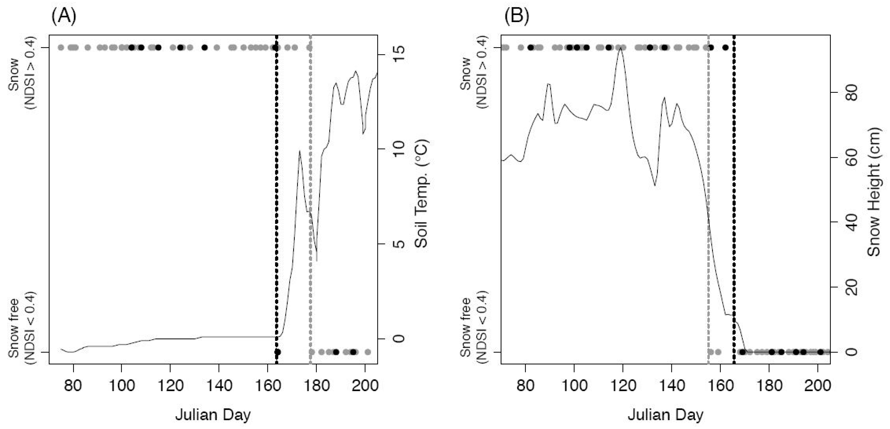
3.2. Vegetation Data and Ground Measurements of Snowmelt

We assembled a database of 1272 vegetation plots from subalpine grasslands, shrub and heathlands, and alpine meadows. Data were provided by the Conservatoire Botanique National Alpin (http://www.cbn–alpin.fr/) and the Ecrins National Park. Floristic surveys were conducted from 2000 to 2014 and consisted of recording all vascular plants occurring in a sampled area ranging from 10 m2 to 25 m2. The geo-location error of vegetation plots was less than 10 m. Vegetation plots below 1800 m a.s.l. were disregarded in order to exclude grassland patches interspersed with mountain forests.
Similarity-based cluster analysis was conducted using an agglomerative clustering technique [59]. First, floristic distances between vegetation plots were estimated using the Jaccard index, which is based on presence–absence data. Second, k clusters of vegetation plots were defined using the Partitioning Around Medoids (PAM) algorithm implemented in the pam function of the R package version 1.15.3 [60,61]. The resulting k clusters minimize the sum of dissimilarities between groups. Exploratory analyses were conducted using a prescribed number of clusters ranging from five to thirty. We identified that twelve clusters represented a fair compromise between having enough vegetation plots per cluster and adequately capturing plant community diversity in the targeted area. The floristic compositions of the resulting clusters are consistent with previous vegetation studies conducted in these mountain ranges [62].
Hourly soil temperatures in high elevation grasslands were recorded using miniaturized data loggers (Hobo pendant®, Onset, Cape Cod, MA, USA) buried at 5 cm depth. During snow covered periods, subsurface soil temperatures did not exhibit circadian variations and temperature remained between –0.5 °C and 0.5 °C throughout the day. When snow melt-out occurs, daily amplitude increases significantly and the mean daily temperature rapidly rises above 0 °C. Our visual inspection of snow cover on a few instrumented sites clearly indicated that disappearance of snow coincides with the rise of subsurface soil temperature.
Snow depth measurements for 2013 and 2015 were obtained from (i) the Nivose network of Météo France consisting of high-altitude automatic weather stations; and (ii) from two automatic stations belonging to the experimental site of Col du Lac Blanc (2720 m a.s.l., Grandes Rousses range). At all stations, snow depth measurements were collected hourly using an ultra-sonic snow depth gauge.

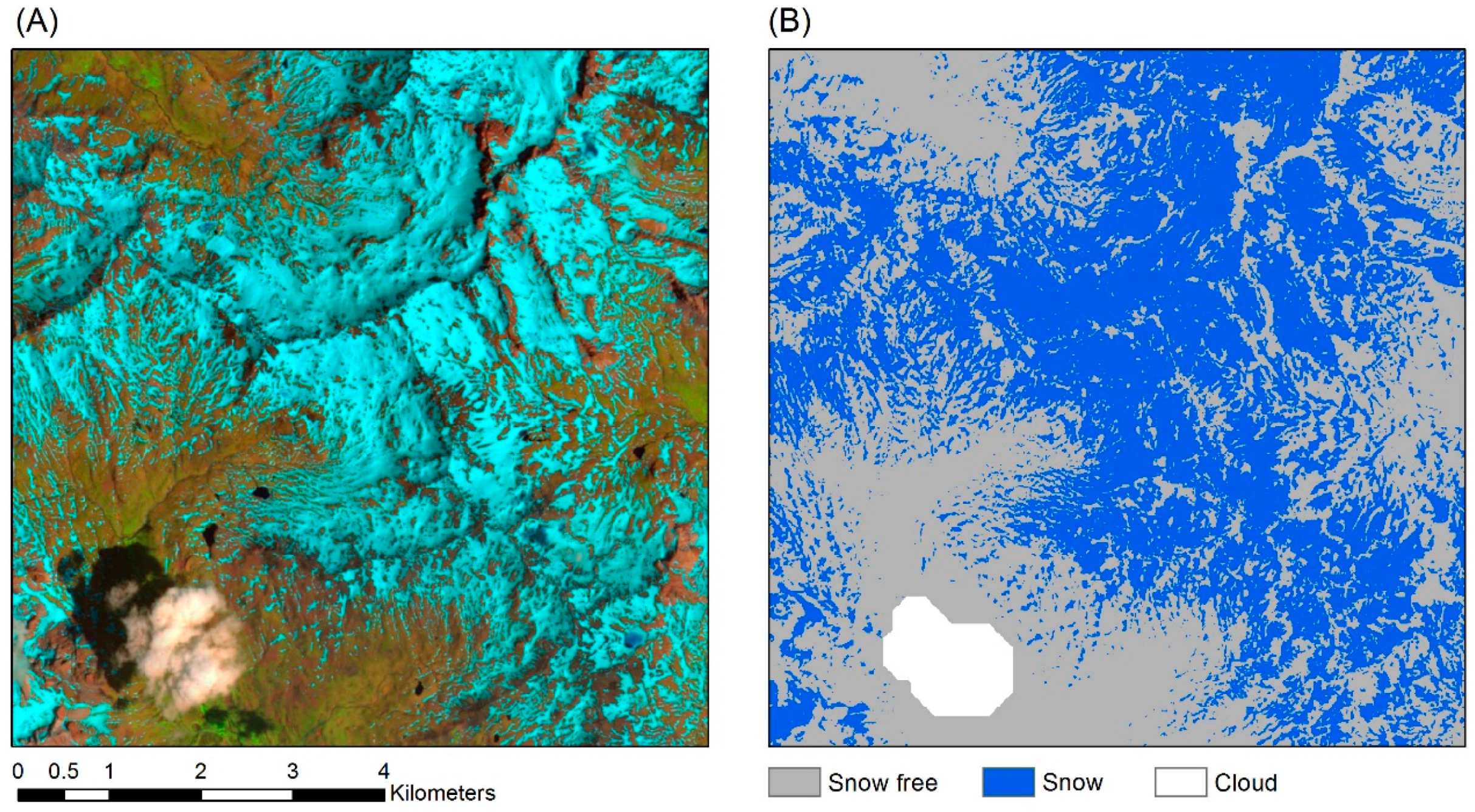
3.3. Validation of Snow Cover Maps

Time series of snow cover maps derived from MODIS and from SPOT-4/5 and Landsat-8 (hereafter shortened to SL) were used to estimate the first snow free day for available ground measurements in 2013 and 2015. Eight (eleven) time series of soil temperature and four (seven) time series of snow height were available for 2013 and 2015, respectively. Time series of snow cover maps from MODIS and SL imagery were extracted for ground validation points for both years, and the median date between the last observation of snow cover (NDSI > 0.4) and the first snow free observation (NDSI < 0.4) was used to estimate the first snow free day in Julian Days. Considering that both ground-based and remote sensing based estimates were subject to error, standardized major axis regression [63] was used to fit a linear relationship between ground measurements and MODIS and SL estimates of first snow free day. R-squared was used to assess the strength of the relationship between remote sensing observations and ground-based measurements. Mean uncertainty was calculated for both MODIS and SL images and was defined as the average number of days between the last observation of snow cover and the first snow free observation. Mean error was estimated for both medium and high resolution imagery and was defined as the average difference in Julian Days between remote sensing and ground-based observations of snow melt-out.

3.4. Mapping First Snow Free Day and Peak NDVI

We selected 2015 as an example year to carry out regional-scale mapping of the first snow free day and peak NDVI, and to explore the relevance of these maps for differentiating alpine plant community habitat. Images for 2015 consisted of eleven SPOT-5 scenes and twelve Landsat-8 scenes from 23 March to 8 September 2015 (Table S1). Given that no-data values were possible due to cloud cover or shadows, only pixels that were above 1800 m a.s.l., non-forested and that contained more than eleven non-NA observations were retained for analysis (n = 4,580,421). The same algorithm described above was used to estimate the first snow free day (Julian Day) for each pixel, based on the median date between the last observation of snow cover and the first snow free observation. Pixels which were snow free before the first available image (23 March) were set to no-data. The resulting map of the first snow free day was exported at 25 m resolution. NDVI at peak standing biomass (NDVImax) was also estimated for each pixel by extracting the yearly maximum observed value of NDVI. The same protocol was used to estimate the first snow free day and NDVImax using MODIS imagery for 2015, which was available from 1 February to 30 September (n = 44,642). Given the large number of MODIS observations, it was not necessary to remove pixels based on the number of cloud-free observations. Pearson’s r was used to test for linear correlations between elevation (m a.s.l.) and the first snow free day (Julian Day), and between elevation and NDVImax for a random sample of 5000 pixels iterated 100 times for both MODIS and SPOT and Landsat estimates of first snow free day. Lastly, first snow free day and NDVImax were extracted for all vegetation plots for the year 2015, using both MODIS and SL time series maps. We anticipated an overall negative relationship between first snow free day and NDVImax, with the expectation that a shorter growing season will lead to reduced peak standing biomass.

4. Results

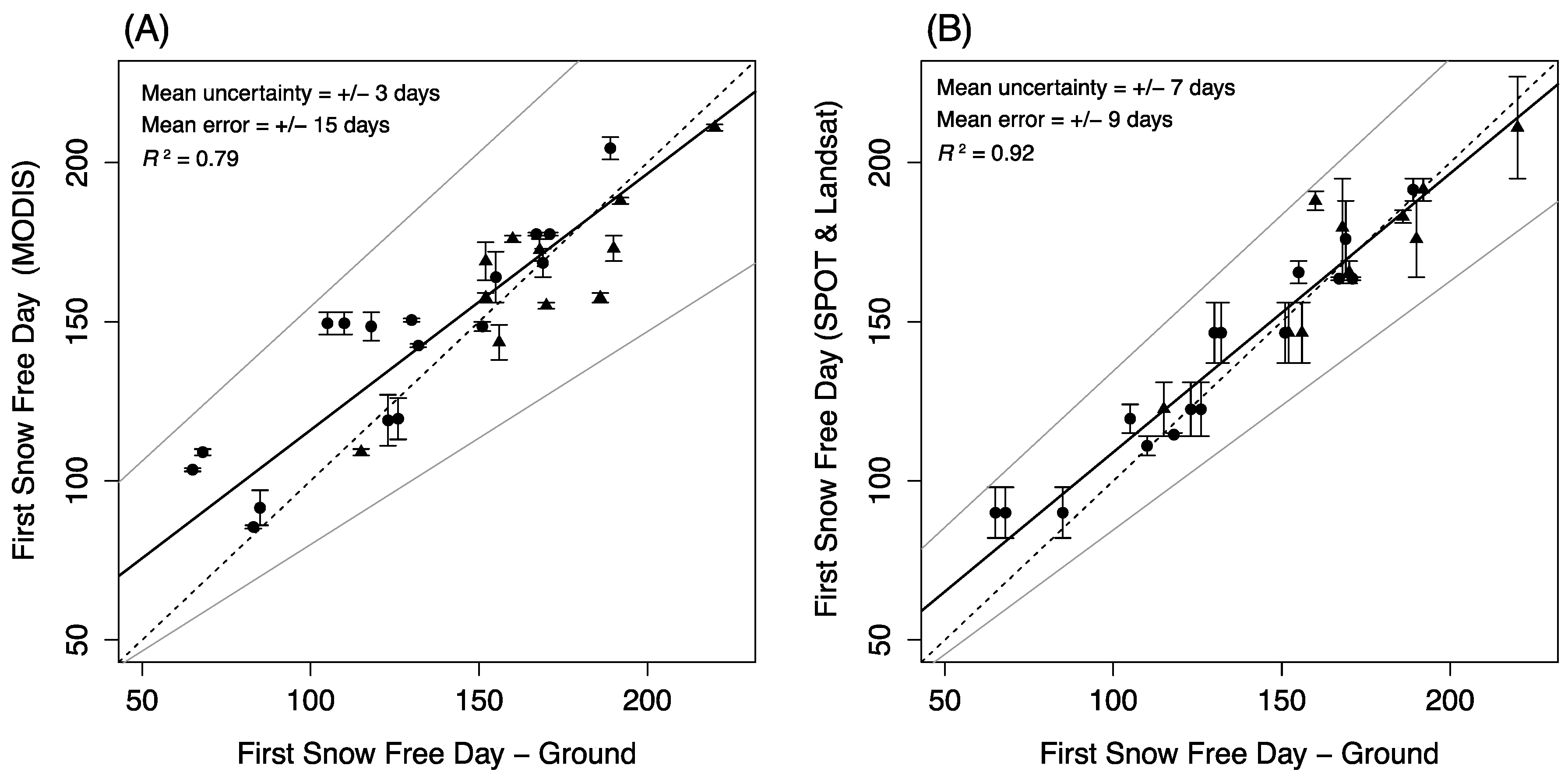
4.1. Validation of Remote Sensing Estimates of the First Snow Free Day

Overall, ground-based physical measures of snow melt-out showed strong agreement with remote sensing observations. The date at which soil temperatures passed above 0 °C and at which snow height reached 0 cm corresponded with NDSI values passing below 0.4, especially in the case of SPOT-4/5 and Landsat-8 and (SL) imagery (Figure 6 and Figure 7). For the soil temperature plot shown in Figure 6A, MODIS (grey dashed line) overestimated the first snow free day relative to the soil temperature logger, whereas in Figure 6B, MODIS underestimated the first snow free day as determined by snow height. In both cases, topographic heterogeneity within 250 m pixels led to discrepancy between ground-based measurements of snow melt-out and NDSI observed by MODIS. The examples provided in Figure 6 demonstrate that if high spatial resolution images are available at the critical timing of snowmelt, it is possible to precisely determine the first snow free day even in topographically heterogeneous sites. The increased temporal resolution of MODIS relative to SL was evident due to the higher frequency of snow cover observations (Figure 6).

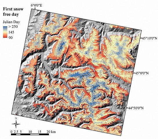
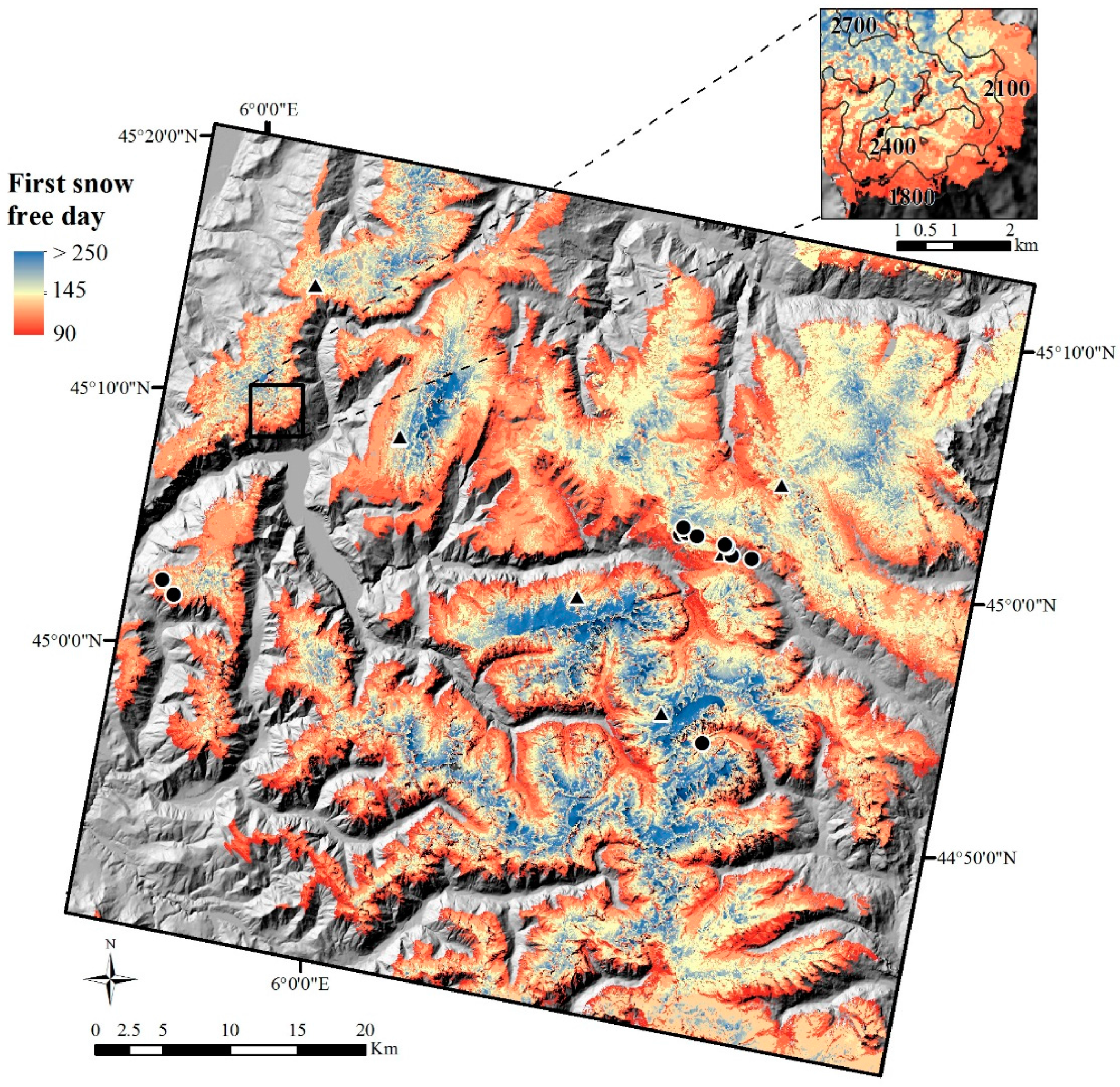
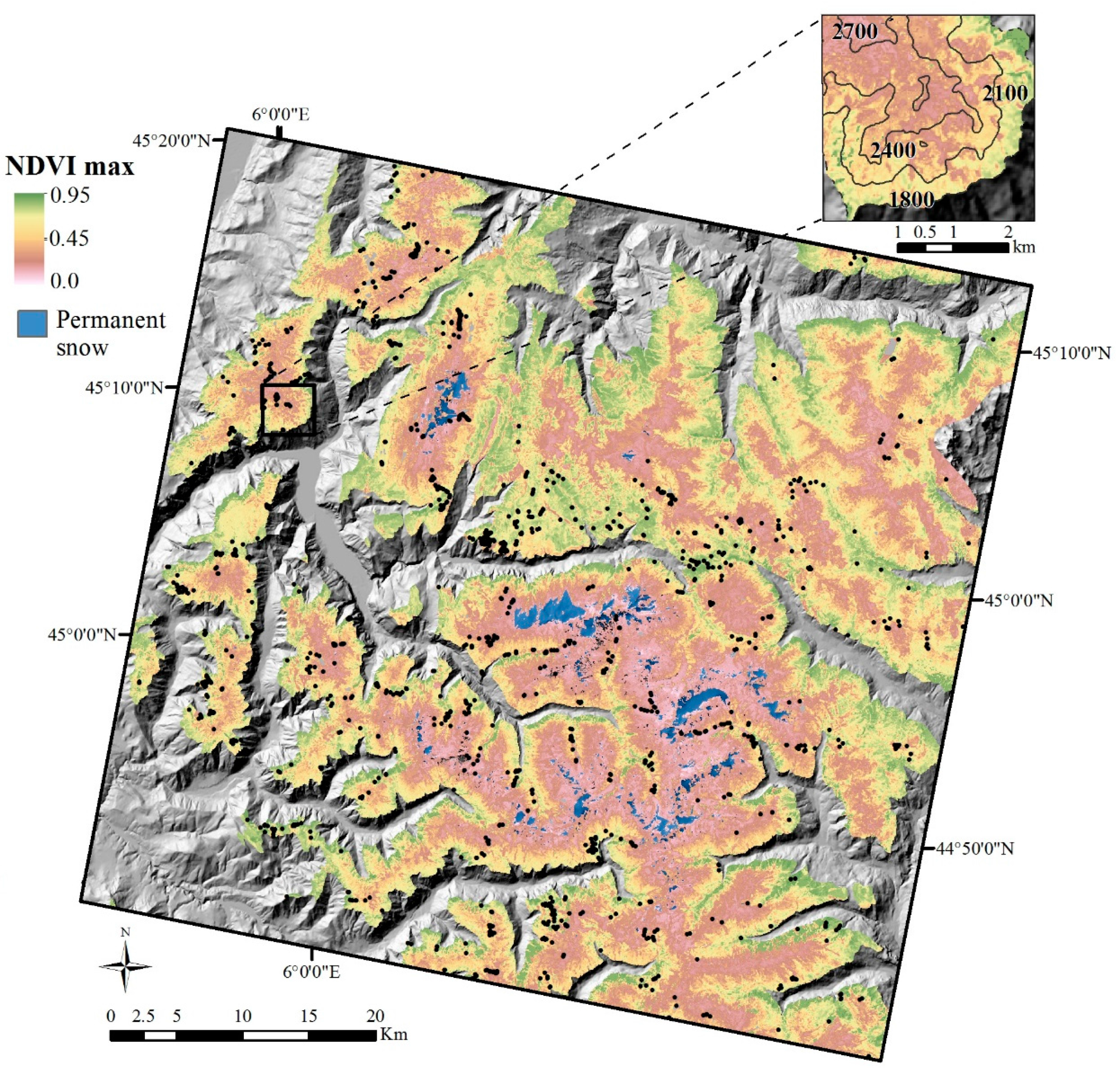
4.2. Mapping the First Snow Free Day and Peak NDVI at the Regional Scale

Estimates of the first snow free day for 2015 varied from 31 March (Julian Day 90) to 4 September (Julian Day 247; Figure 8) for SL imagery and between 10 February (Julian Day 41) and 29 September (Julian Day 272) for MODIS imagery. The first snow free day was significantly correlated with elevation in the case of both MODIS and SL imagery; however, the correlation was stronger in the case of MODIS (0.76 as compared to 0.57 for SL imagery). Despite the overall positive trend between elevation and the first snow free day, we found substantial variation (up to 90 days) in melt-out timing along elevation isolines due to changes in slope orientation (Figure 8 inset). We considered changes in the first snow free day for similar elevations to represent the local effects of wind and topographic heterogeneity.
For MODIS imagery, peak NDVI (NDVImax) varied from 0 to 0.85 with a mean of 0.48. When estimated with SL imagery, NDVImax varied from 0 to 0.95 with a mean of 0.51 (Figure 9). Maximum values of NDVI above 0.90 (which represented the 0.95 quantile for SL imagery) likely reflected the localized presence of tree cover, despite our effort to remove these pixels from the analysis, or in isolated cases could have been the result of errors in cloud masks. The negative correlation between NDVImax and elevation was somewhat stronger for MODIS than for SL imagery (−0.81 vs. −0.73). The inset in Figure 9 illustrates the high heterogeneity in NDVImax at 25 m resolution, which reflects the patchy distribution of plant communities in high-elevation landscapes.

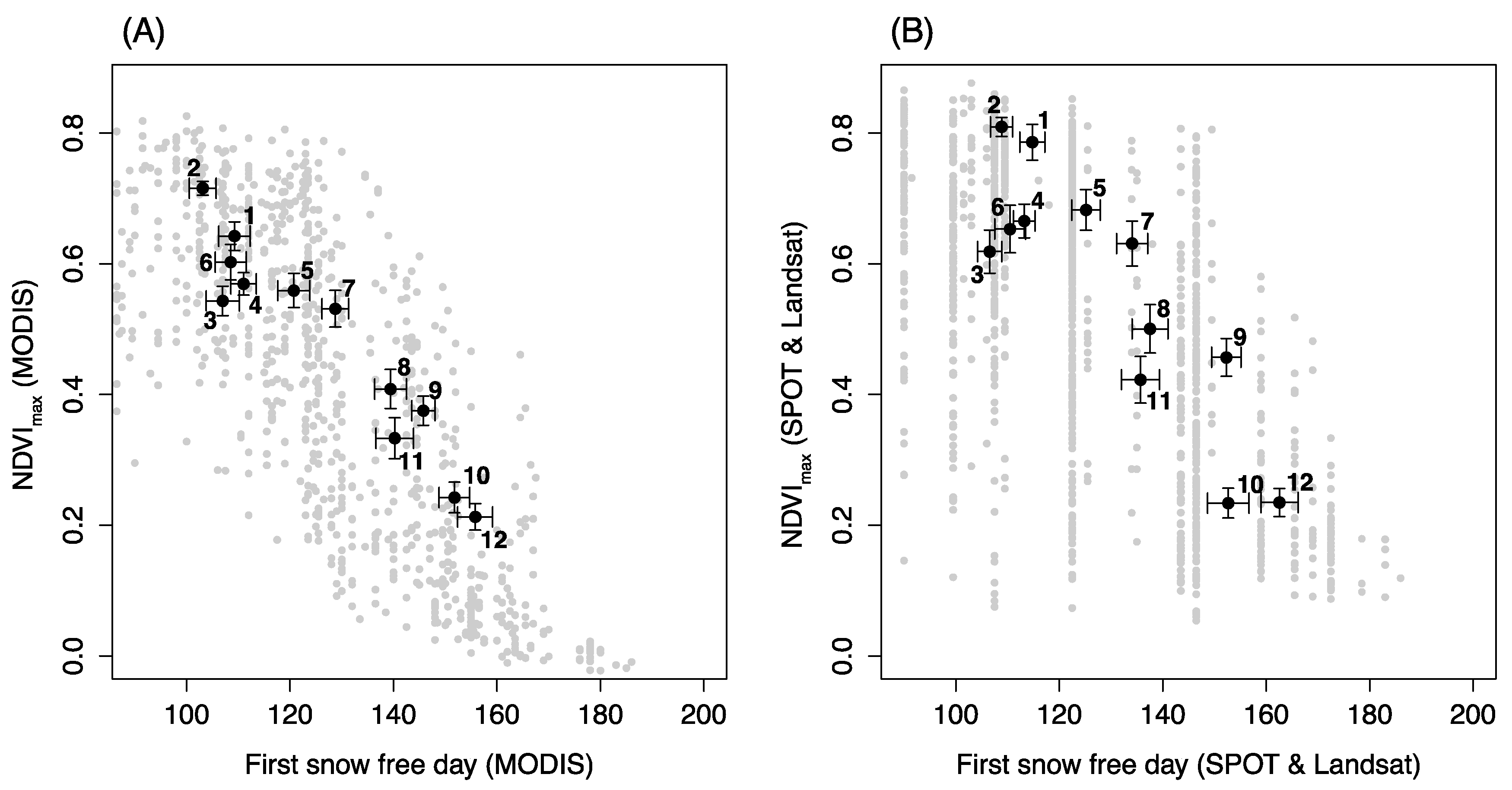
4.3. Differentiating Alpine Plant Community Habitat by Peak NDVI and the First Snow Free Day

Dominant high-elevation plant communities were differentiated relative to the first snow free day and peak NDVI (NDVImax; Figure 10). The distribution of plant communities with respect to the first snow free day and NDVImax was similar for axes derived from both MODIS and SL imagery, reflecting the turnover of plant communities along an elevation gradient. The higher temporal resolution of MODIS imagery was apparent due to a more continuous snow melt-out gradient, whereas SL imagery resulted in clustered points as a function of scene acquisition dates (Table S1). Estimation of NDVImax at 25 m with SL imagery resulted in a general upward shift in NDVI values as compared to MODIS at 250 m (Figure 9 and Figure 10), likely due to the higher fraction of vegetation cover contained within smaller pixels.
Subalpine grassland and shrub communities characterized by early snowmelt (Julian Day 100 to 110) and high NDVI (0.5 to 0.80) included communities 1, 2, 3, 4 and 6 (Figure 10; Table 2). Community 5, representing alpine dwarf shrub habitat, became snow free around Julian Day 120 with an NDVImax between 0.55 (MODIS) and 0.70 (SL). Moist subalpine to low-alpine grasslands (community 7), representative of a transition between subalpine and alpine vegetation, became snow free by Julian day 130 and displayed an NDVImax slightly lower than community 5. Communities 8, 9 and 11 corresponded to alpine grasslands occurring at similar elevations, including mesic alpine meadows, alpine snowbed and wind-blown, dry alpine meadows. As estimated by MODIS, these groups shared similar values of the first snow free day around Julian Day 140 and NDVImax around 0.4. SL imagery increased differentiation of alpine grassland communities, especially in the case of snowbed vegetation (community 9), along the first snow free day axis. Lastly, communities 10 and 12 were representative of talus and scree vegetation with low NDVI around 0.2 and a first snow free day after Julian day 150 (Figure 10; Table 2).

5. Discussion

Our study proposes a simple method for estimating first snow free day from time series of multispectral imagery, which we validate for both high and moderate spatial resolution sensors with respect to ground measurements of snow melt-out date. We further demonstrate the ability of first snow free day and peak NDVI derived from high-resolution imagery to capture the floristic diversity of mountain plant communities located above the tree line. Although improving process-based models of snow accumulation and snowmelt in complex mountain terrain is an ongoing priority for snow scientists [64,65,66], and is necessary to forecast the effects of climate change on snow cover duration [21], simulating spatial heterogeneity of snowmelt in topographically complex study areas remains a difficult task [67,68]. Remote sensing thus represents a promising avenue for observing snow distribution patterns at regular intervals and over large spatial extents.

5.1. On the Importance of High-Resolution Time Series Imagery for Snow Cover Mapping

Optimized pre-processing routines are important to generate accurate output products in mountainous environments [69]. Taking these considerations into account, the SPOT-4/5 and Landsat-8 data pre-processed by CNES-Cesbio were made available with the choice of level 2A with surface reflectance correction (L2A-SRE), or with added slope correction to retrieve flat reflectance (L2A-FRE). The benefit of L2A-FRE processing is to ensure temporal consistency of surface reflectance values between SPOT-4/5 and Landsat-8 snow products. Furthermore, the SPOT (Take 5) Experiment generated Sentinel-2 proxy data by simulating high temporal (five-day) and spatial (10 m) resolution scene acquisition. These features are important given the spatial heterogeneity of snow cover duration widely observed in rugged terrain (Figure 2 and Figure 5). For MODIS snow cover maps, the benefits of high temporal resolution for snow cover mapping were apparent in the form of low temporal uncertainty (Figure 6 and Figure 7). Accuracy was somewhat lower as compared to SL imagery, however, due to the relatively coarse spatial resolution of MODIS data, even after enhancement to 250 m resolution using the MODImLab process. Our results point to the importance of both high temporal and spatial resolution multispectral imagery for accurate monitoring of local-scale snow cover distribution and melting processes.

5.2. Perspectives on the Use of High-Resolution Imaery in Alpine Plant Ecology

Plant ecologists interested in modeling responses of alpine vegetation to environmental gradients require information on snow cover duration at the scale of observed turnover in plant communities, which typically occurs over distances <50 m in heterogeneous alpine environments (Figure 2 and Figure 5) [29]. Figure 6A demonstrates the potential for high-resolution imagery to detect snow melt-out timing as determined by soil temperature for an alpine meadow community characteristic of topographically complex ridge crests, which is less accurately measured using moderate resolution imagery (MODIS). Although MODIS did not perform as well as high-resolution imagery, the enhanced snow cover product at 250 m resolution nonetheless showed strong agreement ground observations of snow melt-out (Figure 6 and Figure 7). Our results thus support the use of MODIS, particularly for broad-scale phenological studies that take full advantage of the daily re-visit capacity, e.g., [70]. Finer studies of plant diversity patterns, however, would be better supported using snow cover information derived from high-resolution imagery.
For alpine ecologists, the new opportunities provided by high-resolution imagery are twofold. First, high-resolution data will increase our ability to carry out fine-scale mapping of high-elevation habitats over biogeographical scales. Previous attempts to map mountain habitats above the tree line have been fundamentally limited by the coarse resolution of source data [71]. Most importantly, there have been very few modeling studies accounting for snow cover dynamics in predicting spatial distribution of alpine plants and alpine communities, although see [72], which is rather surprising given that alpine plant ecologists have long recognized the pivotal role of snow cover for plant distribution [73]. In this study, we show that the first snow free day and the vegetation greenness during peak standing biomass provide a two-dimensional habitat template in which one can distinguish the dominant vegetation communities above the tree line. In particular, the effects of mesotopography, i.e., elevation-independent topographic variability, on plant community composition are better captured when high spatial resolution data are used, as evidenced by the increased differentiation of snowbed communities (community 9) in Figure 10B. Ideally, a third axis consisting of exposure to mid-winter and spring frost events caused by frigid air temperatures and a shallow or absent snow pack would be used to further differentiate alpine plant community habitat. Field studies suggest that frost stress has a strong effect on alpine plant growth and community composition [23,74]. Acquiring this information from satellite imagery is challenging, however, due to shadows present in mid-winter imagery and also lack of information on snowpack height.
Second, high spatial and temporal resolution imagery will allow for testing of hypotheses relating plant diversity to ecosystem functioning at an unprecedented scale [75]. For example, time-integrated values of NDVI have been used as a surrogate for aboveground primary productivity in mountainous environments [27,76]. High-resolution data will enable relating these optically-derived proxies of ecosystem functioning to community-scale diversity metrics, whether taxonomic or functional. In addition, there will be new possibilities to investigate how inter-annual variability in snow cover duration cascades into ecosystem functioning and to what extent these dynamics are modulated by the plant composition of grasslands. Up to now, these relationships have been addressed with some disconnect between remote sensing and community ecology disciplines. We believe that the availability of high-resolution data may foster new lines of research in which plant community organization will be fully accounted for in diversity–climate relationships at regional or continental scales.

6. Conclusions

Through ground validation and comparison with moderate resolution products, our study demonstrates the utility of high-resolution time series imagery for mapping snow cover duration in alpine environments. In line with the objectives of the SPOT (Take 5) Experiment, our findings indicate the potential for data made available by the recently launched Sentinel-2 satellite to improve monitoring of snow cover dynamics and plant phenology in temperate alpine regions, which is an important task in the context of ongoing climate change. Specifically, we found that (i) high spatial resolution imagery improves estimates of local differences in snow melt-out induced by topographic heterogeneity; and (ii) that high temporal resolution remains essential in order to precisely detect snow melt-out timing and to capture peak productivity of alpine vegetation during the growing season. Regional-scale maps of the first snow free day and peak NDVI account for turnover in alpine plant communities in our study area and enable snow-vegetation studies at scales beyond what would be feasible using field measurements. The upcoming launch of new satellites (Sentinel-2B, Sentinel-3B Venµs) will continue to increase the availability of high spatial and temporal resolution multispectral imagery, which will improve the accuracy of time series studies dedicated to climate and ecological applications and allow for enhanced monitoring of snow and vegetation dynamics in mountain regions.

Supplementary Materials

The following are available online at https://www.mdpi.com/2072-4292/8/6/481/s1, Table S1: List of satellite images available for 2013 and 2015.

Acknowledgments

The SPOT (Take 5) Experiments were proposed by CESBIO and implemented by CNES with the support of the European Space Agency. We are grateful to CNES for the selection of our SPAMN (SPOT-4) and ECRINS (SPOT-5) projects as test sites for the SPOT (Take 5) Experiments. Data were processed and delivered by CNES for the THEIA Land Data center and the authors wish to highly thank Olivier Hagolle from Cesbio-CNES for the pre-processing of SPOT-4, SPOT-5 and Landsat-8 images and his reviewing of the image processing section of the paper. The MODIS Level-1B data were processed by the MODIS Adaptive Processing System (MODAPS) and the Goddard Distributed Active Archive Center (DAAC), which are archived and distributed by the Goddard DAAC. We thank the Météo France technical staff for maintaining instruments at the Col du Lac Blanc and in the Nivose network, and for handling data acquisition and storage. We thank Deborah Verfaillie (CNRM-GAME, CEN) for providing outputs of the S2M reanalysis. We thank Alexis Mikolajczak who assisted us in preparing vegetation plot data, and Cédric Dentant who provided data from the Ecrins National Park. We thank Jean-Paul Laurent for the monitoring of snow cover dynamics at the Lautaret pass in the framework of the FLUXALP project funded by the Labex OSUG@2020 (Investissements d’avenir—ANR10 LABX56). Thanks are also due to Vincent Thiérion from the National Institute for Environmental Science and Research (IRSTEA) for his technical help on the SPOT-4 part of the project, to Amélie Arnould for her contribution to the climate figures, and to Thomas Cavallo for his work on snow mapping with SPOT-4 images. Pascal Sirguey thanks the University of Otago, the Grenoble Institute of Technology (INP-Grenoble) and the University Grenoble-Alpes (UGA) for supporting his contribution to this work while on research and study leave in Grenoble. Finally, the authors thank the reviewers of this paper for their constructive comments on an earlier version of the manuscript. This research was conducted on the long-term research site Zone Atelier Alpes, a member of the ILTER-Europe network, and was supported by the Zone Atelier Alpes and by the Station Alpine J. Fourier (SAJF). The publication was funded by the Gestion et Impacts du Changements Climatique, Drôme: Eau, Climat Impacts liés aux Changements (GICC-DECLIC) program.

Author Contributions

Jean-Pierre Dedieu coordinated the SPAMN and ECRINS SPOT-Take 5 projects, supervised the paper, and was in charge of image processing and the snow mapping task. Bradley Z. Carlson carried out snow mapping, performed validation of snow cover maps, and analyzed plant communities with respect to available imagery. Sylvain Bigot was in charge of the climate data and analysis, and coordinated the GICC-DECLIC program. Pascal Sirguey developed the MODImLab toolbox and provided the expertise for processing of MODIS imagery. Philippe Choler provided data from soil temperature loggers, performed statistical analysis of vegetation data, and supervised the alpine ecology section of the paper. Vincent Vionnet provided data from snow height monitoring stations, analyzed data from the S2M reanalysis and assisted with the analysis of remote sensing and ground observations. The writing was led by Jean-Pierre Dedieu and Bradley Z. Carlson. All authors contributed to the manuscript.

Conflicts of Interest

The authors declare no conflict of interest.

References

  1. PCC Report. Working Group 1 Contribution to the IPCC Fifth Assessment Report, Climate Change 2013: The Physical Science Basis; Cambridge University Press: Cambridge, UK, 2013; p. 1535. [Google Scholar]
  2. Armstrong, R.L.; Brun, E. Snow and Climate. In Physical Processes, Surface Energy Exchanges and Modeling; Cambridge University Press: Cambridge, UK, 2010; p. 256. [Google Scholar]
  3. Braun, L.; Weber, M.; Schülz, M. Consequences of climate change for runoff from Alpine regions. Ann. Glaciol. 2000, 31, 19–25. [Google Scholar] [CrossRef]
  4. Seastedt, T.R.; Bowman, W.D.; Caine, T.N.; Mc Knight, D.; Townsend, A.; Williams, M.W. The landscape continuum: A model for high-elevation ecosystems. Bioscience 2004, 54, 111–121. [Google Scholar] [CrossRef]
  5. EEA Report No 12/2012: Climate Change, Impacts and Vulnerability in Europe; European Environment Agency (EEA): Copenhagen, Denmark, 2012. [CrossRef]
  6. Barnett, T.P.; Adam, J.C.; Lettenmaier, D.P. Potential impacts of warming climate on water availability in snow-dominated regions. Nature 2005, 438, 303–309. [Google Scholar] [CrossRef] [PubMed]
  7. Beniston, M.; Uhlmann, B.; Goyette, S.; Lopez-Moreno, J. Will snow abundant winters still exist in the Swiss Alps in an enhanced greenhouse climate? Int. J. Climatol. 2010, 31, 1257–1263. [Google Scholar] [CrossRef]
  8. Bavay, M.; Lehning, M.; Jonas, T.; Löwe, H. Simulations of future snow cover and discharge in Alpine headwater catchment. Hydrol. Processes. 2009, 23, 95–108. [Google Scholar] [CrossRef]
  9. Hantel, M.; Hirt-Wielke, L. Sensitivity of Alpine snow cover to European temperature. Int. J. Climatol. 2007, 27, 1265–1275. [Google Scholar] [CrossRef]
  10. Gehrig-Fasel, J.; Guisan, A.; Zimmermann, N.E. Tree line shifts in the Swiss Alps: Climate change or land abandonment? J. Veg. Sci. 2007, 18, 571–582. [Google Scholar] [CrossRef]
  11. Améztegui, A.; Brotons, L.; Coll, L. Land-use changes as major drivers of mountain pine (Pinus uncinata Ram.) expansion in the Pyrenees. Glob. Ecol. Biogeogr. 2010, 19, 632–641. [Google Scholar]
  12. Pauli, H.; Gottfried, M.; Dullinger, S.; Abdaladze, O.; Akhalkatsi, M.; Alonso, J.L.B.; Ghosn, D. Recent plant diversity changes on Europe’s mountain summits. Science 2012, 336, 353–355. [Google Scholar] [CrossRef] [PubMed] [Green Version]
  13. Hüsler, F.; Jonas, T.; Riffler, M.; Musial, J.P.; Wunderle, S. A satellite-based snow cover climatology (1985–2011) for the European Alps derived from AVHRR data. Cryosphere 2014, 8, 73–90. [Google Scholar] [CrossRef]
  14. Brown, R.D. Northern Hemisphere snow cover variability and change. J. Clim. 2000, 13, 2339–2355. [Google Scholar] [CrossRef]
  15. Lemke, P.; Ren, J.; Alley, R.B.; Allison, I.; Carrasco, J.; Flato, G.; Fujii, Y.; Kaser, G.; Mote, P.; Thomas, R.H.; et al. Observations changes in snow, ice and frozen ground. In Climate Change 2007: The Physical Science Basis. Contribution of Working Group I to the Fourth Assessment Report of the Intergovernmental Panel on Climate Change; Cambridge and New York University Press: New York, NY, USA, 2007; pp. 337–384. [Google Scholar]
  16. Parajka, J.; Blösch, G. Validation of MODIS snow cover images over Austria. Hydrol. Earth Syst. Sci. 2006, 10, 679–689. [Google Scholar] [CrossRef]
  17. Notarnicola, C.; Duguay, M.; Moelg, N.; Schellenberger, T.; Tetzlaff, A.; Monsoro, R.; Costa, A.; Steurer, C.; Zebisch, M. Snow Cover Maps from MODIS Images at 250 m Resolution, Part 1: Algorithm Description. Remote Sens. 2013, 5, 110–126. [Google Scholar] [CrossRef]
  18. Beniston, M. Is snow in the Alps receding or disappearing? WIREs Clim. Chang. 2012. [Google Scholar] [CrossRef]
  19. Szczypta, C.; Gascoin, S.; Houet, T.; Hagolle, O.; Dejoux, J.F.; Vigneaux, C.; Fanise, P. Impact of climate and land cover changes on snow cover in a small Pyrenean catchment. J. Hydrol. 2015, 521, 84–99. [Google Scholar] [CrossRef] [Green Version]
  20. Dedieu, J.P.; Lessard-Fontaine, A.; Ravazzani, G.; Cremonese, E.; Shalpykova, G.; Beniston, M. Shifting mountain snow patterns in a changing climate from remote sensing retrieval. Sci. Total Environ. J. 2014, 493, 1267–1279. [Google Scholar] [CrossRef] [PubMed]
  21. Randin, C.F.; Dedieu, J.P.; Zappa, M.; Long, L.; Dullinger, S. Validation of and comparison between a semi distributed rainfall-runoff hydrological model (PREVAH) and a spatially distributed snow evolution model (SnowModel) for snow cover prediction in mountain ecosystems. Ecohydrology 2015, 8, 1181–1193. [Google Scholar] [CrossRef]
  22. Körner, C. CO2 exchange in the alpine sedge Carex curvula as influenced by canopy structure, light and temperature. Oecologia 1982, 53, 98–104. [Google Scholar] [CrossRef]
  23. Choler, P. Consistent shifts in alpine plant traits along a mesotopographical gradient. Arctic. Antarct. Alp. Res. 2005, 37, 444–453. [Google Scholar] [CrossRef]
  24. Carlson, B.Z.; Choler, P.; Renaud, J.; Dedieu, J.P.; Thuiller, W. Modelling snow cover duration improves predictions of functional and taxonomic diversity for alpine plant communities. Ann. Bot. 2015, 116, 1023–1034. [Google Scholar] [CrossRef] [PubMed]
  25. Fisk, M.C.; Schmidt, S.K.; Seastedt, T.R. Topographic patterns of above-and below ground production and nitrogen cycling in alpine tundra. Ecology 1998, 79, 2253–2266. [Google Scholar] [CrossRef]
  26. Jonas, T.; Rixen, C.; Sturm, M.; Stoeckli, V. How alpine plant growth is linked to snow cover and climate variability. J. Geophys. Res. Biogeosci. 2008, 113, G03013. [Google Scholar] [CrossRef]
  27. Choler, P. Growth response of temperate mountain grasslands to inter-annual variations in snow cover duration. Biogeosciences 2015, 12, 3885–3897. [Google Scholar] [CrossRef]
  28. Freppaz, M.; Williams, B.L.; Edwards, A.C.; Scalenghe, R.; Zanini, E. Simulating soil freeze/thaw cycles typical of winter alpine conditions: Implications for N and P availability. Appl. Soil Ecol. 2007, 35, 247–255. [Google Scholar] [CrossRef]
  29. Billings, W.D. Arctic and alpine vegetations: Similarities, differences, and susceptibility to disturbance. BioScience 1973, 23, 697–704. [Google Scholar] [CrossRef]
  30. Scherrer, D.; Körner, C. Topographically controlled thermal-habitat differentiation buffers alpine plant diversity against climate warming. J. Biogeogr. 2011, 38, 406–416. [Google Scholar] [CrossRef]
  31. Carlson, B.Z.; Randin, C.F.; Boulangeat, I.; Lavergne, S.; Thuiller, W.; Choler, P. Working toward integrated models of alpine plant distribution. Alp. Bot. 2013, 123, 41–53. [Google Scholar] [CrossRef] [PubMed]
  32. Klein, A.G.; Barnett, A.C. Validation of daily MODIS snow cover maps of the Upper Rio Grande River Basin for the 2000–2001 snow year. Remote Sens. Environ. 2003, 86, 162–176. [Google Scholar] [CrossRef]
  33. Fontana, F.; Rixen, C.; Jonas, T.; Aberegg, G.; Wunderle, S. Alpine grassland phenology as seen in AVHRR, VEGETATION, and MODIS NDVI time series-a comparison with in situ measurements. Sensors 2008, 8, 2833–2853. [Google Scholar] [CrossRef] [Green Version]
  34. Molotch, N.P.; Margulis, S.A. Estimating the distribution of snow water equivalent remotely sensed snow cover data and a spatially distributed snowmelt model: A multi-resolution, multi-sensors comparison. Adv. Water Rerour. 2008, 31, 1503–1514. [Google Scholar] [CrossRef]
  35. Hagolle, O.; Sylvander, S.; Huc, M.; Claverie, M.; Clesse, D.; Dechoz, C.; Lonjou, V.; Poulain, V. SPOT-4 (Take 5): Simulation of Sentinel-2 Time Series on 45 Large Sites. Remote Sens. 2015, 7, 12242–12264. [Google Scholar] [CrossRef]
  36. Bonet, R.; Arnaud, F.; Bodin, X.; Bouche, M.; Boulangeat, I.; Bourdeau, P.; Bouvier, M.; Cavalli, L.; Choler, P.; Delestrade, A.; et al. Indicators of climate: Ecrins National Park participates in long-term monitoring to help determine the effects of climate change. Ecol. Mont-J. Prot. Mount. Areas Res. 2016, 8, 44–52. [Google Scholar] [CrossRef]
  37. Wiscombe, W.J.; Warren, S.G. A model for the spectral albedo of snow. I—Pure snow. J. Atmos. Sci. 1980, 37, 2712–2733. [Google Scholar] [CrossRef]
  38. Dozier, J.; Painter, T. Multispectral and hyperspectral remote sensing of alpine snow properties. Annu. Rev. Earth Planet Sci. 2004, 32, 465–494. [Google Scholar] [CrossRef]
  39. Rees, W.G. Remote Sensing of Snow and Ice; Taylor & Francis, CRC Press Book: Cambridge, UK, 2006; p. 285. [Google Scholar]
  40. Riano, D.; Chuvieco, E.; Salas, J.; Aguado, I. Assessment of different topographic corrections in Landsat-TM data for mapping vegetation types. IEEE Trans. Geosci. Rem. Sens. 2003, 41, 1056–1061. [Google Scholar] [CrossRef]
  41. Menzel, A.; Sparks, T.H.; Estrella, N.; Aasa, A.; Ahas, R.; Alm-Kübler, K.; Bissolli, P.; Braslavska, O.; Briede, A.; Chmielewski, F.; et al. European phenological response to climate change matches the warming pattern. Glob. Chang. Biol. 2006, 12, 1969–1976. [Google Scholar] [CrossRef]
  42. Durand, Y.; Giraud, G.; Laternser, M.; Etchevers, P.; Mérindol, L.; Lesaffre, B. Reanalysis of 47 years of climate in the French Alps (1958–2005): Climatology and trends for snow cover. J. Appl. Meteorol. Climatol. 2009, 48, 2487–2512. [Google Scholar] [CrossRef]
  43. Auer, I.; Böhm, R. HISTALP—Historical instrumental climatological surface time series of the Greater Alpine Region. Int. J. Climatol. 2007, 27, 17–46. [Google Scholar] [CrossRef]
  44. Durand, Y.; Laternser, M.; Giraud, G.; Etchevers, P.; Lesaffre, B.; Mérindiol, L. Reanalysis of 44 years of climate in the French Alps (1958–2002): Methodology, model validation, climatology, and trends for air temperature and precipitation. J. Appl. Meteorol. Climatol. 2009, 48, 429–449. [Google Scholar] [CrossRef]
  45. Gobiet, A.; Kotlarsky, S.; Beniston, M.; Heinrich, G.; Rajczak, J.; Stoffel, M. 21st century climate change in the European Alps—A review. Sci. Total Environ. 2014, 493, 1138–1151. [Google Scholar] [CrossRef] [PubMed]
  46. Vionnet, V.; Brun, E.; Morin, S.; Boone, A.; Faroux, S.; Le Moigne, P.; Martin, E.; Willemet, J.M. The detailed snowpack scheme Crocus and its implementation in SURFEX v7.2. Geosci. Model Dev. 2012, 5, 773–791. [Google Scholar] [CrossRef] [Green Version]
  47. Hagolle, O.; Huc, M.; Villa Pascual, D.; Dedieu, G. A multi-temporal and multispectral method to estimate aérosol optical tickness over land, for the atmospheric correction of FormoSat-2, Venµs and Sentinel-2 images. Remote Sens. 2015, 7, 2668–2691. [Google Scholar] [CrossRef]
  48. Dymond, J.R.; Shepherd, J.D. Correction of the topographic effect in remote sensing. IEEE Trans. Geosci. Remote Sens. 1999, 37, 2618–2620. [Google Scholar] [CrossRef]
  49. Shepherd, J.D.; Dymond, J.R. Correcting satellite imagery for the variance of reflectance and illumination with topography. Int. J. Remote Sens. 2003, 24, 3503–3514. [Google Scholar] [CrossRef]
  50. Hall, D.K.; Riggs, G.; Salomonson, V.; Di Girolamo, N.; Bayr, K. Modis snow-cover products. Remote Sens. Environ. 2002, 83, 181–194. [Google Scholar] [CrossRef]
  51. Hall, D.K.; Riggs, G. Accuracy assessment of the MODIS snow-cover products. Hydrol. Process. 2007, 21, 1534–1547. [Google Scholar] [CrossRef]
  52. Sirguey, P.; Mathieu, R.; Arnaud, Y. Subpixel monitoring of the seasonal snow cover with MODIS at 250 m spatial resolution in the Southern Alps of New Zealand: Methodology and accuracy assessment. Remote Sens. Environ. 2009, 113, 160–181. [Google Scholar] [CrossRef]
  53. Dumont, M.; Gardelle, J.; Sirguey, P.; Guillot, A.; Six, D.; Rabatel, A.; Arnaud, Y. Linking glacier annual mass balance and glacier albedo retrieved from MODIS data. Cryosphere 2012, 6, 1527–1539. [Google Scholar] [CrossRef] [Green Version]
  54. Mary, A.; Dumont, M.; Dedieu, J.P.; Durand, Y.; Sirguey, P.; Milhem, H.; Mestre, O.; Negi, H.S.; Kokhanovsky, A.A.; Lafaysse, M.; et al. Intercomparison of retrieval algorithms for the specific surface area of snow from near-infrared satellite data in mountainous terrain, and comparison with the output of a semi-distributed snowpack model. Cryosphere 2013, 7, 741–761. [Google Scholar] [CrossRef]
  55. Sirguey, P.; Mathieu, R.; Arnaud, Y.; Khan, M.; Chanussot, J. Improving MODIS spatial resolution for snow mapping using wavelet fusion and ARSIS concept. IEEE Geosci. Remote Sens. Lett. 2008, 5, 78–82. [Google Scholar] [CrossRef] [Green Version]
  56. Dozier, J. Spectral signature of alpine snow cover from the Landsat Thematic Mapper. Remote Sens. Environ. 1989, 28, 9–22. [Google Scholar] [CrossRef]
  57. Ackerman, S.; Strabala, K.; Menzel, W.; Frey, R.; Moeller, C.; Gumley, L. Discriminating clear sky from clouds with MODIS. J. Geophys. Res. 1998, 103, 32141–32157. [Google Scholar] [CrossRef]
  58. Levin, N.; Shmida, A.; Levanoni, O.; Tamari, H.; Kark, S. Predicting mountain plant richness and rarity from space using satellite-derived vegetation indices. Divers. Distrib. 2007, 13, 692–703. [Google Scholar] [CrossRef]
  59. Kaufman, L.; Rousseeuw, P.J. Finding Groups in Data: An Introduction to Cluster Analysis; John Wiley & Sons: Hoboken, NJ, USA, 2009; p. 368. [Google Scholar]
  60. Maechler, M.; Rousseeuw, P.; Struyf, A.; Hubert, M.; Hornik, K. Cluster: Cluster Analysis Basics and Extensions. R Package Vers. 2014, 2, 56. [Google Scholar]
  61. R Core Team. R: A Language and Environment for Statistical Computing; R Foundation for Statistical Computing: Vienna, Austria, 2015. [Google Scholar]
  62. Choler, P.; Michalet, R. Niche differentiation and distribution of Carex curvula along a bioclimatic gradient in the southwestern Alps. J. Veg. Sci. 2002, 13, 851–858. [Google Scholar] [CrossRef]
  63. Warton, D.I.; Duursma, R.A.; Falster, D.S.; Taskinen, S. Smatr 3—An R package for estimation and inference about allometric lines. Methods Ecol. Evol. 2012, 3, 257–259. [Google Scholar] [CrossRef]
  64. Mott, R.; Schirmer, M.; Bavay, M.; Grünewald, T.; Lehning, M. Understanding snow-transport processes shaping the mountain snow-cover. Cryosphere 2010, 4, 545–559. [Google Scholar] [CrossRef]
  65. Winstral, A.; Marks, D.; Gurney, R. Simulating wind-affected snow accumulations at catchment to basin scales. Adv. Water Resour. 2013, 55, 64–79. [Google Scholar] [CrossRef]
  66. Vionnet, V.; Martin, E.; Masson, V.; Guyomarc’h, G.; Bouvet, F.N.; Prokop, A.; Lac, C. Simulation of wind-induced snow transport and sublimation in alpine terrain using a fully coupled snowpack/atmosphere model. Cryosphere 2014, 8, 395–415. [Google Scholar] [CrossRef] [Green Version]
  67. Egli, L.; Jonas, T.; Grünewald, T.; Schirmer, M.; Burlando, P. Dynamics of snow ablation in a small Alpine catchment observed by repeated terrestrial laser scans. Hydrol. Process. 2012, 26, 1574–1585. [Google Scholar] [CrossRef]
  68. Revuelto, J.; Vionnet, V.; López-Moreno, J.I.; Lafaysse, M.; Morin, S. Combining snowpack modeling and terrestrial laser scanner observations improves the simulation of small scale snow dynamics. J. Hydrol. 2016, 533, 291–307. [Google Scholar] [CrossRef]
  69. Teillet, P.M.; Guindon, B.; Goodeonugh, D.G. On the slope aspect correction of multispectral scanner data. Can. J. Remote Sens. 1982, 8, 84–106. [Google Scholar] [CrossRef]
  70. Li, Z.; Yu, G.; Xiao, X.; Li, Y.; Zhao, X.; Ren, C.; Fu, Y. Modeling gross primary production of alpine ecosystems in the Tibetan Plateau using MODIS images and climate data. Remote Sens. Environ. 2007, 107, 510–519. [Google Scholar] [CrossRef]
  71. Mücher, C.A.; Klijn, J.A.; Wascher, D.M.; Schaminée, J.H. A new European Landscape Classification (LANMAP): A transparent, flexible and user-oriented methodology to distinguish landscapes. Ecol. Ind. 2010, 10, 87–103. [Google Scholar] [CrossRef]
  72. Randin, C.F.; Vuissoz, G.; Liston, G.E.; Vittoz, P.; Guisan, A. Introduction of snow and geomorphic disturbance variables into predictive models of alpine plant distribution in the Western Swiss Alps. Arctic. Antarct. Alp. Res. 2009, 41, 347–361. [Google Scholar] [CrossRef]
  73. Walker, D.A.; Halfpenny, J.C.; Walker, M.D.; Wessman, C.A. Long-term studies of snow-vegetation interactions. BioScience 1993, 43, 287–301. [Google Scholar] [CrossRef]
  74. Wipf, S.; Stoeckli, V.; Bebi, P. Winter climate change in alpine tundra: Plant responses to changes in snow depth and snowmelt timing. Clim. Chang. 2009, 94, 105–121. [Google Scholar] [CrossRef]
  75. Violle, C.; Reich, P.B.; Pacala, S.W.; Enquist, B.J.; Kattge, J. The emergence and promise of functional biogeography. Proc. Natl. Acad. Sci. USA 2014, 111, 13690–13696. [Google Scholar] [CrossRef] [PubMed]
  76. Rossini, M.; Cogliati, S.; Meroni, M.; Migliavacca, M.; Galvagno, M.; Busetto, L.; Cremonese, E.; Julitta, T.; Siniscalco, C.; di Cella, U.M.; et al. Remote sensing-based estimation of gross primary production in a subalpine grassland. Biogeosciences 2012, 9, 2565–2584. [Google Scholar] [CrossRef] [Green Version]
Figure 1. Location of study area, showing the overall SPOT-4 (Take 5) extent and the reduced SPOT-5 extent in yellow, which covers the Oisans massif and the Ecrins National Park. The red star shows the Figure 2 location and the red inset shows the “Massif des Cerces” area of Figure 5. The background image is a visible and infrared color composition (green, near infra-red and short-wavelength infrared channels) from a SPOT-4 scene acquired on 14 April 2013, with snow cover shown in blue. ©CNES-Cesbio.
Remotesensing 08 00481 g001
Figure 2. Photo of spring snowmelt near the Col du Lautaret (Figure 1), showing characteristic spatial heterogeneity in snow cover duration and the differential timing of plant green-up. ©Philippe Choler/Station Alpine Joseph-Fourier.
Remotesensing 08 00481 g002
Figure 3. Inter-annual variability between 1959 and 2015 of annual average air temperature (°C) and precipitation rate (mm/day) at 850 hPa in the French Alps, which is roughly equivalent to 1500 m a.s.l.. Data were obtained from the NCEP-NCAR (National Centers for Environmental Prediction/National Center for Atmospheric Research). Anomalies were calculated based on the 1961–1990 average; the alpine regional index is approximately 5.5°–6.8°E/44.5°–46°N. Vertical dashed black lines indicate the years considered in our study (2013 and 2015).
Remotesensing 08 00481 g003
Figure 4. The first snow free day (in Julian Day) for different elevations in the Oisans mountain range from SAFRAN-SURFEX/Crocus-MEPRA model chain (S2M). Vertical dashed red lines indicate the years considered in our study (2013 and 2015).
Remotesensing 08 00481 g004
Figure 5. Example snow cover map based on the Normalized Difference Snow Index (NDSI) for a 56 km2 in the Massif des Cerces (location provided in Figure 1), for 5 June 2015. (A) Visible and infrared color composite retrieved from a SPOT-5 image at 10 m resolution, showing snow cover in light blue; and (B) map of snow cover showing snow (blue), snow free areas (grey) and cloud/shadow cover (white) derived from a SPOT-5 image ©CNES-Cesbio.
Remotesensing 08 00481 g005
Figure 6. Time series observations for (A) a wind-blown dry alpine meadow dominated by Kobresia mesuroides located at 2648 m a.s.l. for 2013; and (B) a snow height monitoring station located in a topographic depression at 3100 m a.s.l. in the commune of La Grave for 2015. In (A), the line indicates running mean daily measures of soil temperature (°C, k = 3). In (B), the line indicates running mean daily measures of snow pack height (cm, k = 3). Solid grey points show MODIS observations of snow cover, while solid black points show SPOT-5 and Landsat-8 observations of snow cover. The black dashed vertical line represents first snow free day estimated by SPOT and Landsat imagery, and the grey dashed vertical line represents the first snow free day estimated by MODIS.
Remotesensing 08 00481 g006
Figure 7. Ground-based measurements plotted relative to remote sensing-based estimates of the first snow free day for 28 observations in 2013 and 2015. Circles correspond to the first snow free day measured by soil temperature, and triangles correspond to first snow free day measured by snow height. Position on the y-axis represents the median Julian Day between the last snow and the first snow free observations (shown with error bars), as estimated by (A) MODIS; and (B) SPOT-5 and Landsat-8. The dashed line is the 1:1 trend line, whereas the solid line is the result of a standardized major axis regression between ground-based measurements and remote sensing observations. Grey lines indicate upper and lower confidence intervals for slope and intercept estimates.
Remotesensing 08 00481 g007
Figure 8. The first snow free day estimated using SPOT-5 and Landsat-8 imagery for 2015, expressed in Julian Days. Pixels have a 25 m spatial resolution and correspond to alpine areas above 1800 m a.s.l.. Points show the location of soil temperature loggers (circles) and snow height monitoring stations (triangles). The inset shows variation in snow cover duration relative to elevation isolines.
Remotesensing 08 00481 g008
Figure 9. Peak NDVI (NDVImax) estimated using SPOT-5 and Landsat-8 imagery for 2015. Pixels have a 25 m spatial resolution and correspond to alpine areas above 1800 m a.s.l. Points show the location of vegetation plots indicated at Section 3.2 (n = 1272). The inset shows variation in NDVImax relative to elevation isolines. Permanent snow cover includes mostly glaciated surfaces.
Remotesensing 08 00481 g009
Figure 10. The first snow free day (Julian Day) and peak NDVI (NDVImax) for 2015 represented by grey dots, measured by (A) MODIS; and (B) SPOT-5 and Landsat-8 images for 1272 vegetation plots. Black points and error bars represent the mean position with confidence intervals of the twelve plant communities detailed in Table 1. Values of NDVI close to 0 represent plant communities occurring in sparsely vegetated screes and talus. The overall upward shift in NDVI values for SPOT-5 and Landsat-8 imagery as compared to MODIS NDVI can be attributed to more homogenous plant cover occurring within smaller pixels. The error bars represent 95% confidence intervals around estimates of mean NDVI max and the first snow free day per plant community.
Remotesensing 08 00481 g010
Table 1. Wavelength characteristics of the spectral bands used to identify snow cover for images acquired by the four sensors employed in this study.
SensorResolution (m)Wavelength (µm)
GreenRedNear-InfraredShortwave Infrared
SPOT-4200.50–0.590.61–0.680.78–0.891.58–1.75
SPOT-5100.50–0.590.61–0.680.78–0.891.58–1.75
Landsat-8300.53–0.590.64–0.670.85–0.881.57–1.65
MODIS5000.54–0.560.62–0.670.84–0.881.63–1.65
Table 2. Dominant co-occurring species and mean elevation (m a.s.l.) and habitat descriptions for twelve plant communities identified by clustering analysis.
CommunityMean ElevationDescriptionDominant Co-Occurring Species
11996Mosaic of subalpine heath, shrub and tall herb communitiesRhododendron ferrugineum, Vaccinium myrtillus, Agrostis agrostiflora, Vaccinium uliginosum, Alnus alnobetula, Juniperus sibirica, Deschampsia flexuosa, Cacalia alliariae, Imperatoria ostruthium, Geranium sylvaticum
22045Tall subalpine grasslands and pasturesFestuca paniculata, Nardus stricta, Meum athamanticum, Festuca nigrescens, Festuca violacea, Trifolium alpinum, Anthoxanthum odoratum, Vaccinium uliginosum, Carex sempervirens, Brachypodium rupestre
32083Dry subalpine to low-alpine meadows (on siliceous bedrocks)Festuca acuminata, Festuca laevigata, Juniperus sibirica, Sempervivum arachnoideum, Carex sempervirens, Helictotrichon parlatorei, Arctostaphylos uva-ursi, Festuca paniculata, Thymus praecox, Hieracium peleterianum
42096Subalpine heathlandsVaccinium myrtillus, Deschampsia flexuosa, Nardus stricta, Festuca paniculata, Carex sempervirens, Juniperus sibirica, Festuca nigrescens, Festuca violacea, Deschampsia.flexuosa, Vaccinium uliginosum, Anthoxanthum odoratum
52159Prostrate alpine dwarf-shrub heathsVaccinium uliginosum, Loiseleuria procumbens, Vaccinium myrtillus, Carex sempervirens, Nardus stricta, Rhododendron ferrugineum, Empetrum nigrum, Juniperus sibirica, Trifolium alpinum, Deschampsia flexuosa
62178Dry subalpine meadows (on non-siliceous bedrocks)Festuca laevigata, Sesleria caerulea, Helictotrichon sedenense, Helianthemum nummularium, Helictotrichon parlatorei, Festuca paniculata, Festuca violacea, Dryas octopetala, Alchemilla alpigena, Thymus praecox
72338Mesic to wet, subalpine to low-alpine pasturesPlantago alpina, Nardus stricta, Festuca violacea, Festuca nigrescens, Salix herbacea, Trifolium thalii, Poa alpina, Leontodon pyrenaicus, Carex sempervirens, Polygonum viviparum
82413Mesic alpine meadowsCarex curvula, Nardus stricta, Carex sempervirens, Gentiana alpina, Plantago alpina, Festuca halleri, Vaccinium uliginosum, Trifolium alpinum, Salix herbacea, Avenula versicolor
92448Alpine snowbed communitiesSalix herbacea, Alchemilla pentaphyllea, Plantago alpina, Omalotheca supina, Carex foetida, Nardus stricta, Luzula alpinopilosa, Alopecurus alpinus, Poa alpina, Sibbaldia procumbens
102507Alpine scree and open meadowsLeucanthemopsis alpina, Cerastium pedunculatum, Saxifraga bryoides, Cacalia leucophylla, Luzula alpinopilosa, Doronicum grandiflorum, Cryptogramma crispa, Veronica alpina, Omalotheca supina, Oxyria digyna
112528Wind-blown, dry alpine meadowsKobresia myosuroides, Festuca halleri, Vaccinium uliginosum, Silene acaulis, Saxifraga bryoides, Juncus trifidus, Dryas octopetala, Carex curvula, Carex rupestris, Salix herbacea
122701Subnival scree vegetationSaxifraga bryoides, Leucanthemopsis alpina, Saxifraga oppositifolia, Silene acaulis, Oxyria digyna, Festuca halleri, Festuca violacea, Geum reptans

