Retrieval of the Absorption Coefficient of L-Band Radiation in Antarctica From SMOS Observations

Abstract

Microwave emissions at the L-band (1–2 GHz) in Antarctica are characterized by a significant contribution of ice layers at great depth, from hundreds to a thousand meters. Brightness temperatures, thus, could provide the internal temperature of the ice sheet. However, there are two difficulties to overcome in developing an accurate retrieval algorithm. First, it is difficult to know precisely from which depths waves are emanating because the ice-absorption coefficient is uncertain at the L-band, despite several formulations proposed in the literature over the past few decades. Second, emissivity potentially varies in Antarctica due to remnant scattering in firn (or ice), even at the Brewster angle, and despite the low frequency, limiting the accuracy of the estimate of the physical temperature. Here, we present a retrieval method able to disentangle the absorption and emissivity effects from brightness temperature over the whole continent. We exploit the fact that scattering and absorption are controlled by different physical parameters and phenomena that can be considered as statistically independent. This independence provides a constraint to the retrieval method, that is then well-conditioned and solvable. Our results show that (1) the retrieved absorption agrees with the permittivity model proposed by Mätzler et al. (2006), and (2) emissivity shows significant variations, up to 6% over the continent, which are correlated with wind speed and accumulation patterns. A possible cause of this latter point is density heterogeneity and sastrugi buried in the firn. These two results are an important step forward for the accurate retrieval of internal temperature using low-frequency microwave radiometers.

1. Introduction

Observation in the microwave range with space-borne radiometers is a rich source of information on surface and subsurface physical properties in Antarctica. The passive-microwave signal emitted from snow and firn mainly depends on grain size [1,2], surface accumulation [3,4], surface temperature [5,6], or melting events [7,8,9]. K and Ka bands (from 18 to 40 GHz) were investigated for decades and were found to be particularly suited to probe the surface and a few meters below. In contrast, microwave emissions from ice sheets at lower frequencies (1–2 GHz, L-band) is characterized by much lower absorption and scattering effects. This major difference represents a potential to retrieve information on the internal structure of the Antarctic ice sheet. The signal measured at L-band depends, among others, on the temperature profile from the surface to approximately 500 to 1500 m down [10]. Retrieving information on temperature is of crucial importance because temperature influences ice motion in two ways. First, the dependence of ice fluidity on temperature is exponential [11], so ice velocity as well. Second, sliding is possible for temperate basal ice, where the water supply of basal melt lubricates the ice–bedrock interface [12,13]. Internal temperature T of the Antarctic ice sheet is directly measured at a few sites, where in situ deep borehole measurements were conducted after deep ice-core drilling [14], but no direct observation is available elsewhere. More specifically, the geothermal flux at the bedrock–ice interface has been estimated either by considering the seismic properties of the crust and upper mantle [15,16], or by assessing the crustal thickness from observations of the magnetic field [17,18]. Significant discrepancies between these datasets were shown, reaching several tens of mW m${}^{-2}$, and up to 50 mW m${}^{-2}$ in West Antarctica [18]. Furthermore, all of these methods intend to constrain the value of the geothermal flux with a geodynamic approach, but a glaciological approach has never been used at a continental scale. Thus, the L-band signal contains worthwhile information on the amount of heat dissipated in the Antarctic ice sheet, which is required to build future projections of the Antarctic ice sheet [19].

Despite the low absorption coefficient of ice in this frequency range, the L-band signal at horizontal polarization is influenced by surface changes such as the formation/disappearance of hoar or changes due to wind events [20,21]. This is not the case at vertical polarization near the Brewster angle, where the brightness temperature is temporally stable over Antarctica [22]. However, it highlights significant spatial variations [10] (Figure 1a). Brightness temperature appears highly correlated with surface temperature (Figure 1b), and a second-order influence of ice thickness has also been revealed [23,24], explained by the vertical profile of temperature. A large part of Antarctic basal ice is at melting point [25], so that the mean vertical temperature gradient is firstly governed by surface temperature and ice thickness, and secondly modulated by vertical and horizontal ice velocities through advection. Hence, physical temperature decreases more slowly with depth over thicker ice. The impact on brightness temperature leads to an indirect dependence on ice thickness. This effect is illustrated by the low brightness-temperature values reported over deep subglacial lakes [23], and in particular at Lake Vostok [26]. A first-order approximation of brightness temperature $T_B$ can be written as follows, neglecting interferences and coherent effects, and assuming absorption largely dominates scattering [27,28,29]:

$$T_B=\eta (T_E+T_b{e}^{-{\int }_0^H\frac{{\kappa }_a(z)}{\mu }dz}).$$

(1)

where $\eta$ is apparent emissivity, H is ice thickness, $\mu =\cos \theta$ with $\theta$ the angle of the refracted direction to the radiometer in the firn and ice, ${\kappa }_a(z)$ the absorption coefficient, and z is the depth below the ice surface. The left term of the sum is the contribution of ice layers, and the right term is the contribution of the underlying bedrock at temperature $T_b$. This right term is generally negligible, except where ice is shallow. Effective temperature $T_E$ corresponds to the weighted contributions of the emitting ice layers, and defined by References [30,31,32]

$$T_E={\int }_0^H\frac{{\kappa }_a(z)}{\mu }T(z)e^{-{\int }_0^z\frac{{\kappa }_a(z^{\prime })}{\mu }d{z}^{\prime }}dz.$$

(2)

where T is the physical ice temperature. At the L-band, scattering and absorption mechanisms have an uneven influence on the signal within the ice body. Near the surface, snow grains and crystals are much more smaller than wavelength (∼${10}^{-1}$ m), so that scattering effects are negligible [33,34]. Firn layering and density variations plays a major role in the control of brightness temperature, each layer interface reflecting a small amount of incoming radiation. Furthermore, since the typical layer thickness is close to the wavelength, interferences appear between the multiple internal reflected radiations [34]. However, these mechanisms have limited impact on $T_B$ observations acquired close to the Brewster angle and at vertical polarisation [35], where the reflection of radiation at the layer interface vanishes. In this case, $\eta$ is expected to be close to 1 and absorption to be the main mechanism affecting brightness temperature at the L-band. Absorption coefficient ${\kappa }_a$ depends on vacuum wavelength $\lambda$ and ice-complex permittivity components $ϵ={ϵ}^{\prime }+i{ϵ}^{″}$. The real part of permittivity is well known (order of magnitude $\sim 1$), and depends mostly on density, and marginally on temperature [36,37]. On the contrary, the imaginary part has very low magnitude ($\sim {10}^{-4}$ to ${10}^{-3}$) making it very difficult to measure. Its dependence on temperature is uncertain. The permittivity model proposed by Mätzler et al. (2006) [38] is, in principle, valid down to 1 GHz, which includes the L band. However another model was proposed by Tiuri et al. (1984) [36] where the imaginary part of the permittivity is three- or fourfold higher, in the range of 840 MHz–12.6 GHz. Using these two permittivity models (hereafter called Mätzler and Tiuri models), and a one-dimensional description of the ice temperature, Macelloni et al. (2016) [10] computed the brightness temperatures at vertical polarisation along three transects on the East Antarctic Plateau, and compared them to the observations acquired by the Soil Moisture and Ocean Salinity (SMOS) satellite. The authors also accounted for density fluctuation within the firn with a stochastic density model [34]. Their results posed a dilemma, since, on the one hand, the $T_B$ values computed with the Tiuri model were only slightly biased while the results with the Mätzler model were affected by a strong warm bias (∼8.5 K); on the other hand, Mätzler model was more sensitive to the ice thickness, poorly visible with Tiuri. As discussed by Macelloni et al. (2016) [10], their temperature profiles were coherent with in situ measurements and three-dimensional simulations, and the physical-parameter uncertainties of the temperature model (surface temperature, geothermal flux, etc.) were not appropriate to induce a strong bias on brightness temperature. At this stage, there are several working hypotheses to progress on this topic:

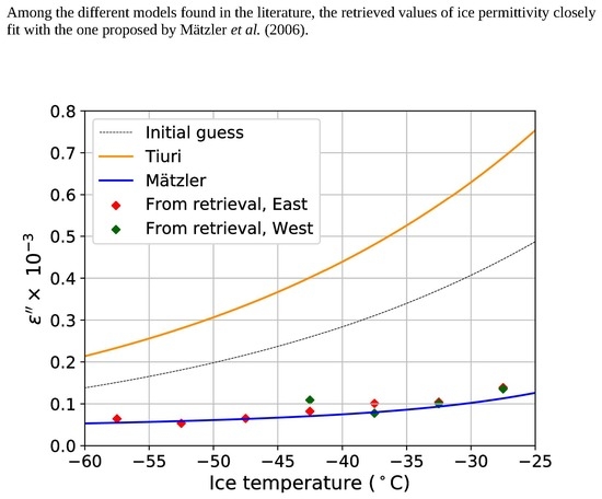
• The Tiuri model is correct, implying that Mätzler absorption is too low. In this case, bias is small and emissivity is very close to 1, which would correspond to negligible scattering effects. The warm bias computed with the Mätzler model is basically due to the overestimation of the deep layers’ contribution to the brightness-temperature signal. However, the Tiuri absorption is too strong to account for apparent spatial variations of the brightness temperature with the ice thickness.
• The Mätzler model is correct, implying that Tiuri absorption is too high. In this case, a mechanism that reduces ice emissivity to explain the warm bias is missing. Surface- and internal-layer roughnesses [39], or snow and firn heterogeneities, are potential sources of reflectivity and scattering that are able to lower emissivity, but they have to be quantified.
• None of the Mätzler and Tiuri models is appropriate, and an intermediate formulation is needed, possibly featuring a different dependence on temperature. Scattering processes should be considered in this case, as in the case of the second hypothesis.

Previous studies explored the first two hypotheses by considering either or more permittivity models as valid [10,23,26,34]. The aim of our study is to explore the last two hypotheses in particular. A method to retrieve absorption and emissivity at a continental scale from SMOS observations is elaborated here. Figure 2 illustrates the flowchart describing the paper methodology: observations and models are introduced in Section 2.1 and Section 2.2, and simulation evaluations are performed in Section 2.3. A simple emission model was applied to retrieve absorption and emissivity in every pixel by minimising an adapted Lagrangian function (Section 2.4.1). Best-fit values were then used to estimate the imaginary part of permittivity, which was compared to existing permittivity models.

2. Materials and Methods

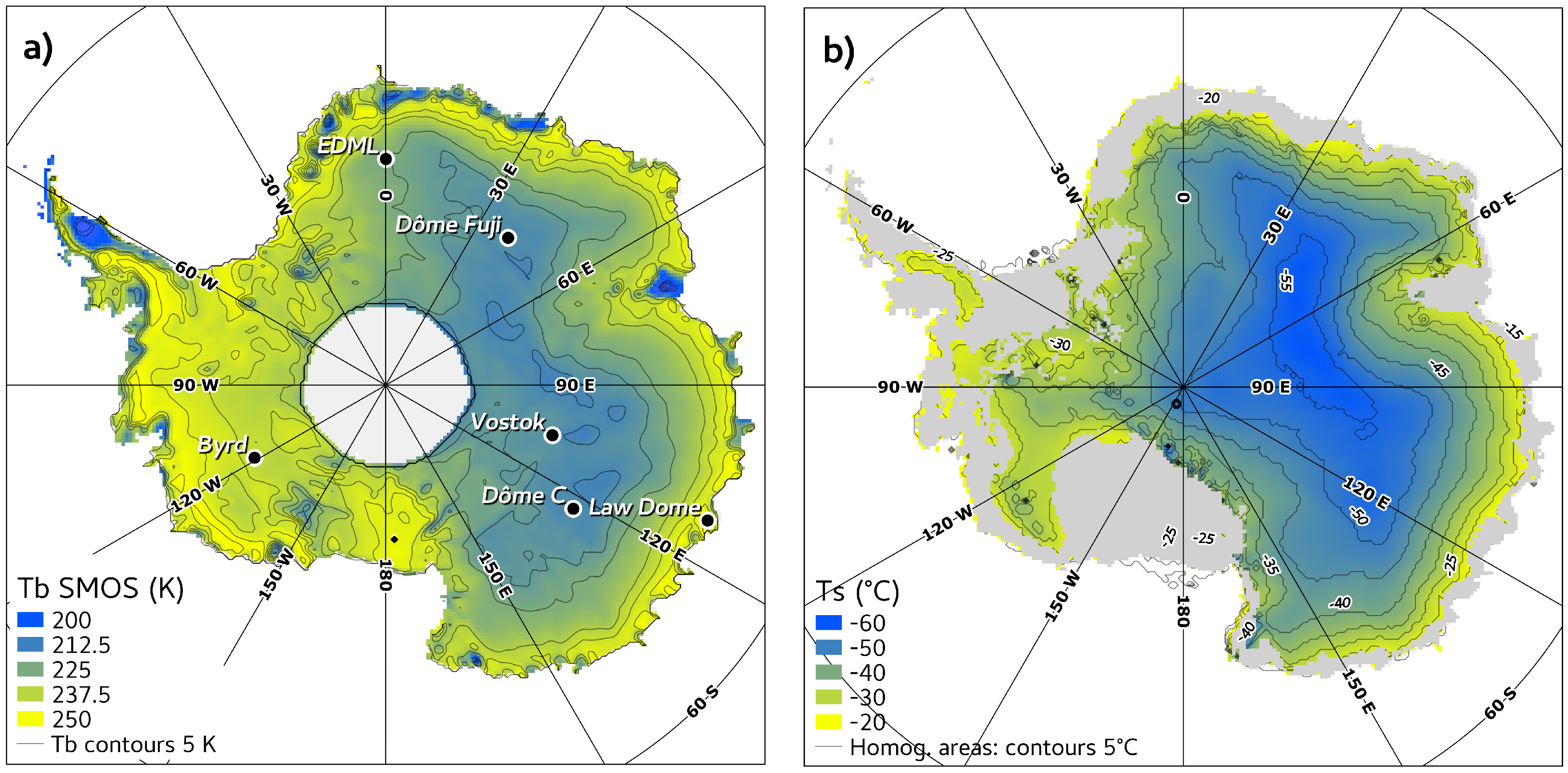
2.1. SMOS Brightness Temperature

Brightness temperature ($T_B$) was measured at L band (1.413 GHz, 21 cm) by a 2D interferometric radiometer carried on board the SMOS satellite [40]. A prerelease of the Level 3 $T_B$ product was used in this study. This dataset is not available online yet, and was provided to us by the CESBIO and CATDS teams for testing (see acknowledgments). The Level 3 product at vertical polarization provides daily brightness temperatures binned every 5${}^{°}$ of incidence angles from 0${}^{°}$ to 65${}^{°}$ [41]. The incident angle bin of 52.5${}^{°}$ is chosen, close to the Brewster angle for ice (∼60${}^{°}$) in order to limit the influence of surface and internal reflections within the firn. The data are gridded on the southern hemisphere azimuthal EASE Grid v2 [42] at the resolution of 25 ×25 km${}^2$. Due to the SMOS orbit, latitudes higher than 85${}^{°}$ were not observed. This Level 3 product is not corrected for atmospheric contributions, because [43] have shown that the water vapor and clouds have a negligible contribution at 1.4 GHz, in general well below 0.1 K.

$T_B$ data were then temporally averaged over a period of 2 years (2013 and 2014, Figure 1a). The expected value of the average of the $n=999\pm 565$ observations for each point had a standard deviation decreasing as $1/\sqrt{n}$, assuming independent observation errors and a stable signal over time, which was the case here. The radiometric precision of a single observation being around 3 K [34], the radiometric precision of the two-year average $T_B$ was of the order of $0.10$ K.

2.2. Temperature Field from the GRISLI Ice-Sheet Model

The physical temperature of ice $T(x,y,z)$ is a critical input of our method, and is provided by the GRISLI 3D ice-sheet thermodynamical model. Version 2.0 of GRISLI benefits from recent improvements concerning the computation of ice flux at the grounding line and a proper description of basal hydrology [44]. Snow and firn are accounted for by considering a weight-equivalent ice slab. The climate parameters forcing the model over time include surface temperature, surface mass balance, basal melt under ice shelves, and sea level (more details in Quiquet et al. (2018) [44]). The accuracy of the final temperature field mainly depends on the geothermal flux at the base of the ice sheet. Several datasets of geothermal flux are available, and the one of Fox-Maule et al. (2005) [17] gives relevant results (Section 2.3). Just as Macelloni et al. (2016) [10], surface temperature ($T_s$) is computed from a temporal average of the Crocus snow model [45], forced by ERA-Interim reanalysis [46] over the 2000–2012 period (Figure 1b). This product was shown to compensate a warm bias in ERA-Interim, compared to the MODIS measurements under clear-sky conditions [47].

The GRISLI model is forced over the last 200,000 years to forget the initial state and to correctly account for the deglaciation signal of the last 20,000 years. The useful model output is the three-dimensional temperature field at present time $T(x,y,z)$, covering both grounded and floating ice, at a resolution of 40 km on 21 vertical layers. Because the simulated ice-sheet topography for the present time is not exactly the observed, a geometrical correction was applied to the 3D temperature field to take into account a thickness bias (Appendix A). This correction was also used for the comparison with measured vertical temperature profiles in the next section. This temperature field was finally regridded on the horizontal EASE Grid v2 to be compared to the $T_B$ product. The relevance of the vertical temperature profiles of GRISLI is discussed in the next section.

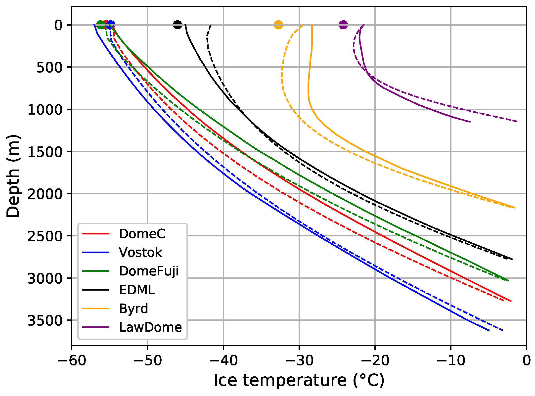
2.3. Borehole Temperature Profiles

Deep borehole temperature profiles are used as control points to evaluate the accuracy of the 3D temperature field produced by GRISLI. Depending on their location on the ice sheet (Figure 1), the profiles show very different shapes, as a consequence of the combined effect of heat diffusion and advection (Figure 3a). On the Antarctic plateau, close or at the ice divide, horizontal velocities are so small that horizontal advection is negligible, and the low surface accumulation leads to limited vertical advection. Accordingly, the vertical temperature profiles are dominated by vertical diffusion and are almost linear with only a slight curvature towards the bedrock: Vostok [48,49], EPICA Dome C (EDC), Dome Fuji [50,51]. In West Antarctica and on the Antarctic coasts, surface accumulation reaches several tens of cms y${}^{-1}$ [4]. Strong horizontal advection from upstream and vertical advection of cold-surface ice toward the bedrock significantly counterbalances heat diffusion from the bedrock toward the surface in the ice bulk. This phenomenon is clearly visible at Byrd [52] and Law Dome [53], where advection and diffusion balance each other, yielding a nearly constant temperature in the upper 1200 m and 700 m at each site respectively. The drill site of EPICA Dronning Maud Land (EDML), located in East Antarctica close to the coast, shows an intermediate type of temperature profile [54]. Note that bedrock-depth accuracy is provided in the Bedmap 2 dataset and is of the order of a few hundred meters, with some areas having a large uncertainty of 1000 m. Compared to this, surface-elevation accuracy is negligible, so that thickness accuracy is practically equal to that of the bedrock.

Over these six drill sites, $T_s$ from Crocus differs from the top temperature of the boreholes by $-0.2\pm 1.3$ K, indicating good accuracy of this dataset for future comparison with $T_B$. On the East Antarctic plateau, the average difference between GRISLI and borehole temperatures is limited to 1 to 2 K on the whole vertical profile (EDC, Dome Fuji, Vostok), and the shape of the profiles are similar. The influence of advection, that gives its remarkable shape to the Byrd profile, is fairly well represented by the model, even if too curved profiles indicate a slightly overestimated advection at Byrd and EDML. The typical shapes of the temperature profiles are well represented. This is necessary to compute plausible effective temperatures and describe their spatial variations.

2.4. Absorption and Emissivity Retrieval

The method to derive the absorption and emissivity in Antarctica is based on a simple forward model (Section 2.4.1) that is used to fit parameters throughout the continent (Section 2.4.2).

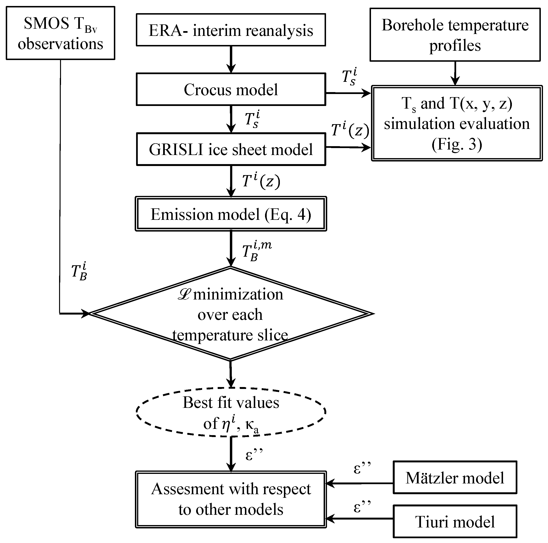
2.4.1. Forward Model

The forward model aims at computing the brightness temperature from a given ice-temperature profile depending on absorption coefficient and emissivity. As the latter two are unknown, it is not possible to use Equations (1) and (2). Equation (2) is rather simplified considering that the dependence of the absorption coefficient on temperature is weak over the range between $T_s$ and $T(z)$ in the upper 1000 m, so that ${\kappa }_a(T(z))\sim {\kappa }_a(\overline{T})$, where $\overline{T}$ is the average value of $T(z)$ over 0–1000 m. Figure 3 shows that the increase of temperature is lower than 7 K, which corresponds to a ${\kappa }_a$ maximum variation of $\pm 10\%$ with the Mätzler model. Dependence of the absorption coefficient on the ice permittivity is described by Reference [30]:

$${\kappa }_a=\frac{4\pi {ϵ}^{″}}{\lambda \sqrt{{ϵ}^{\prime }}}$$

(3)

assuming ${ϵ}^{″}\ll {ϵ}^{\prime }$, as it is the case for ice. Making the dependence to the location on the continent explicit with indices i, and applying the approximation on the absorption, modelled brightness temperature $T_B^{i,m}$ is written as follows [29,31]:

$$T_B^{i,m}={\eta }^i\left({\int }_0^{H^i}\frac{{\kappa }_a}{\mu }{T}^i(z)e^{-\frac{{\kappa }_a}{\mu }z}dz+T_b^i{e}^{-\frac{{\kappa }_a}{\mu }{H}^i}\right).$$

(4)

2.4.2. Retrieval Algorithm

In the following, several sets of thermally homogeneous locations were considered. These sets were designed by slices of the mean temperature on the upper 500 m, since the e-folding depth $1/{\kappa }_a$ is expected to typically range between 100 and 1000 m. These temperature slices range from $-60$ to $-25{}^{°}$C, spaced by 5 ${}^{°}$C. In East Antarctica, these slices correspond to nested rings of a certain altitude range (Figure 1b, contours), and contain between 1500 and 2500 points each (the lower temperature slice only has 672 points). As they are thermally homogeneous, each temperature slice is characterized by a unique value of ${\kappa }_a$. As a consequence, the forward model (Equation (4) written for N points) has one unknown emissivity for each location i and one unknown ${\kappa }_a$, whereas only one observation $T_B^i$ per location is available. The inverse problem thus has more unknowns than independent equations and cannot simply be solved without an additional mathematical constraint. We note, however, that (1) the sole unknown in $T_E^i$ is absorption, and that (2) the apparent emissivity is the only term to depend on scattering. On the one hand, scattering depends on density contrasts between layers (i.e., the density vertical derivative) [34,35], and this can only happen in firn (upper ∼100 m of the ice sheet). On the other hand, absorption depends both on temperature and density [38], and acts significantly over several hundred meters, at least. Thus, both processes are mostly independent, which can be translated into a constraint for the inverse problem as follows. The retrieval of the absorption coefficient and emissivities is performed by minimizing the following Lagrangian function:

$$\mathcal{L}=\underset{\mathcal{J}}{\underbrace{\frac{1}{N}\sum _{i=1}^N{(T_B^{i,m}-T_B^i)}^2}}+\beta \underset{\mathcal{R}}{\underbrace{{\left({\displaystyle \frac{cov(\eta ,T_E)}{{\sigma }_{\eta }{\sigma }_{T_E}}}\right)}^2}}$$

(5)

where ${\sigma }_{\eta }$ and ${\sigma }_{T_E}$ are the standard deviations of $\eta$ and $T_E$ distributions, and $\beta$ is a Lagrange multiplier. N is the number of studied pixels at a given temperature slice. Cost function $\mathcal{J}$ measures the distance of the modelled brightness temperatures to the SMOS observations. Regularisation function $\mathcal{R}$ provides the constraint due to the independence between $\eta$ and $T_E$, noting that the covariance of two random variables approaches zero when they are independent. The covariance of $\eta$ and $T_E$ should be as close to zero as possible compared to the product of their standard deviation ${\sigma }_{\eta }$ and ${\sigma }_{T_E}$. Since this correlation may be negative (anticorrelated variables), $\mathcal{R}$ is designed as its square. Retrieving absorption and emissivity consists of minimizing Lagrangian function $\mathcal{L}$ by using an optimisation algorithm described in detail in Appendix B. Optimization is conducted separately for East and West Antarctica, because the thermal structures of these two ice bodies are completely different (Section 2.3). Furthermore, the regions that undergo summer melt are ruled out of the computation with a mask [9], since the presence of liquid water in the firn greatly impacts the microwave signal. Coastal pixels were not considered for the retrieval method. The imaginary part of permittivity is then deduced from the best fits of ${\kappa }_a$ (Equation (3)), and compared to the models of Tiuri and Mätzler to determine the most valuable approach.

3. Results

3.1. Preliminary Comparison With Borehole Measurements

A preliminary comparison using borehole temperature profiles and the corresponding SMOS brightness temperatures (Figure 3, points at the surface) is particularly enlightening. Equation (2) clearly shows that uncertainties of ice permittivity translates into uncertainties of $T_E$ as much as ice temperature varies with depth, which is site-dependent. At the Byrd site, where the temperature profile is constant over the range of thicknesses significantly contributing to the $T_B$ signal, $T_E$ should be very close to $T_s$ (∼−28 ${}^{°}$C or 245 K) regardless of the value of the absorption coefficient. The resulting $T_B$ is thereby not sensitive to the absorption. Apparent emissivity $\eta$ is then $\eta =T_B/T_s\sim$ 0.98. This does not apply to EDML, EDC, and Dome Fuji, where temperature significantly increases with depth ($T(z)>T_s$). However, in this case, $T_E$ is greater than $T_s$. Given that $T_B$ observed from SMOS was lower than $T_s$, the brightness temperature is significantly lower than $T_E$, by at least several kelvins, whatever the value of the absorption coefficient. As a consequence, apparent emissivity is significantly lower than 1. For several sites of the Antarctica plateau, emissivity spatial variations cannot be ignored to interpret the brightness-temperature signal.

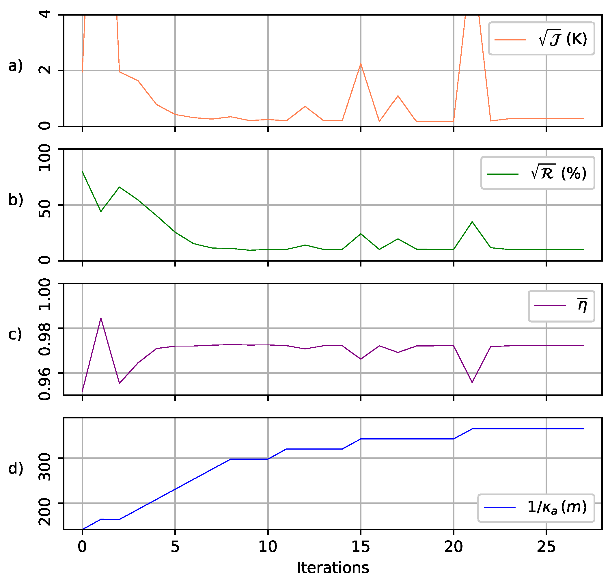
3.2. Lagrangian Function Optimization

The best-fit values were found after tens to hundreds iterations of the optimization algorithm (Appendix B) depending on the temperature slice. Results are shown for e-folding depth $1/{\kappa }_a$, expressed in meters. An example is presented for temperature slice [$-45{}^{°}$C, $-40{}^{°}$C] for East Antarctica (Figure 4). The first correlation values were very high (here, 0.80 for the first iteration, Figure 4b), and this is a consequence of the misestimation of ${\kappa }_a$ at first guess. The consecutive error on the $T_E$ estimations is reported on $\eta$, so that $\mathcal{J}$ is kept low; thereby, $T_E$ and $\eta$ distributions are statistically correlated. Then, the value of $1/{\kappa }_a$ abruptly increased by $1/2$ over the first iteration steps (Figure 4d), indicating that $\mathcal{L}$ had a marked deep minimum in the parameter space. This increase is followed by a decrease of correlation function $\sqrt{\mathcal{R}}$. The emissivity field is iteratively adjusted to these changes in order to satisfy both low-cost and correlation functions as much as possible, and alternations of high and low values appear on the $\sqrt{\mathcal{J}}$ and $\sqrt{\mathcal{R}}$ curves. At the end of the process (Appendix B), the final correlation value ranged between $0.02$ and $0.22$ (

Table 1. Square root of components $\mathcal{J}$ and $\mathcal{R}$ of the Lagrangian function, and corresponding best-fit values of $1/{\kappa }_a$ and $\overline{\eta }$, for each temperature slice (${}^{°}$C), designed by its mean. For the sake of clarity, results are shown for e-folding depth $1/{\kappa }_a$, expressed in meters.

East Ant.	−57.5 ${}^{°}$C	−52.5 ${}^{°}$C	−47.5 ${}^{°}$C	−42.5 ${}^{°}$C	−37.5 ${}^{°}$C	−32.5 ${}^{°}$C	−27.5 ${}^{°}$C
$\sqrt{\mathcal{J}}$ (K)	1.47	1.41	0.80	0.28	0.35	0.66	1.1
$\sqrt{\mathcal{R}}$	0.17	0.22	0.17	0.10	0.03	0.02	0.09
$1/{\kappa }_a$ (m)	466	560	460	365	297	288	216
$\overline{\eta }$	0.989	0.976	0.972	0.972	0.972	0.973	0.978
West Ant.				−42.5 ${}^{°}$C	−37.5 ${}^{°}$C	−32.5 ${}^{°}$C	−27.5 ${}^{°}$C
$\sqrt{\mathcal{J}}$ (K)				1.56	0.96	0.67	0.84
$\sqrt{\mathcal{R}}$				0.09	0.03	0.18	0.15
$1/{\kappa }_a$ (m)				275	319	299	216
$\overline{\eta }$				0.979	0.987	0.986	0.976

). The final value of cost function $\sqrt{\mathcal{J}}$ ranged between $0.28$ K and $1.57$ K. These nonzero values show that a trade-off between $\sqrt{\mathcal{J}}$ and $\sqrt{\mathcal{R}}$ is found by the algorithm, and lower values of $\sqrt{\mathcal{J}}$ would yield higher correlation values.

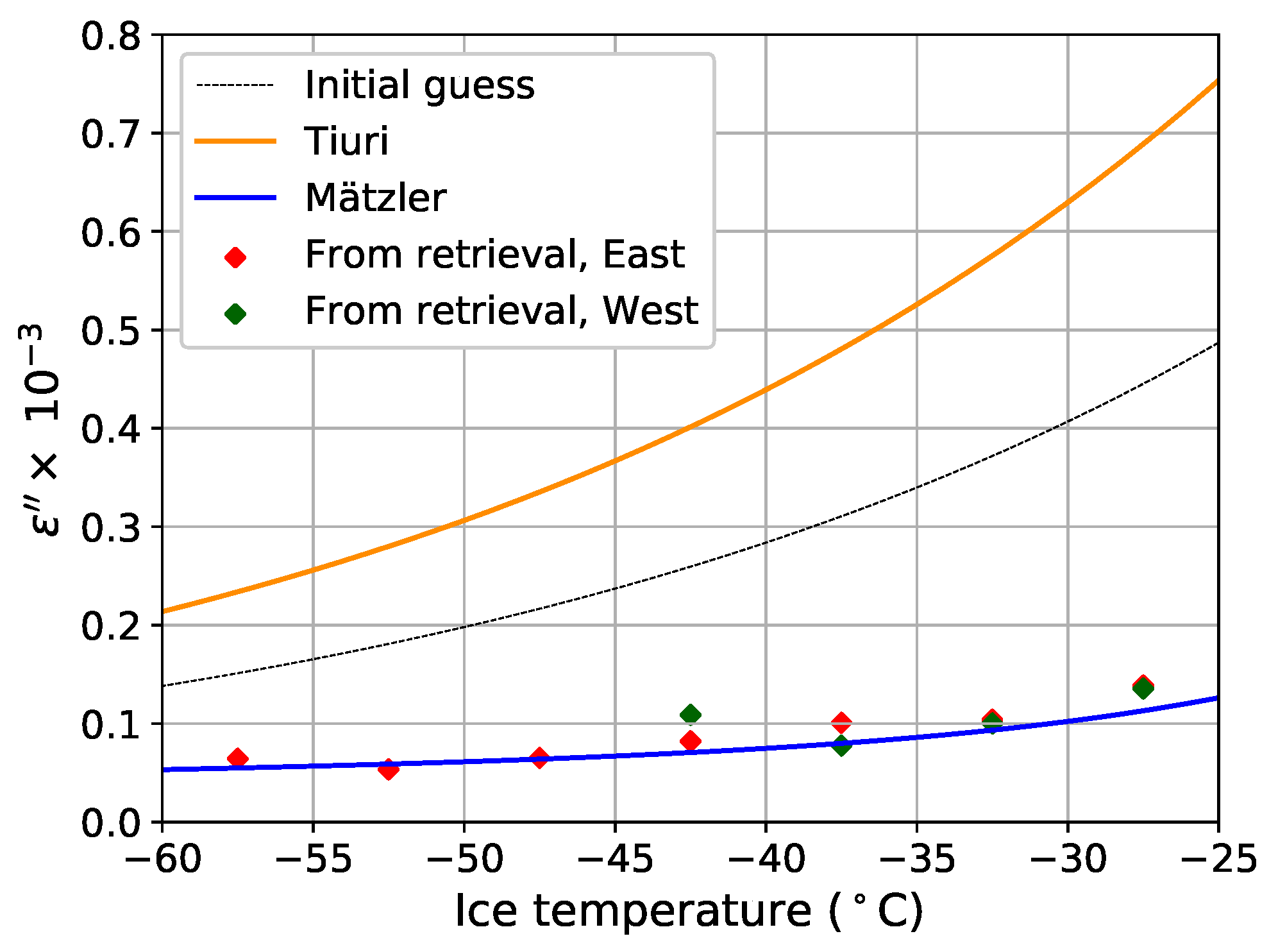
3.3. Absorption Coefficients and Permittivity

The best fit value for the e-folding depth $1/{\kappa }_a$ generally decreases with temperature from 560 to 216 m, (Table 1), as expected from the dependence of ${ϵ}^{″}$ to temperature. Though, the algorithm finds a lower value at $-57.5$ than at $-52.5{}^{°}$C in East Antarctica, and a lower value at $-42.5$ than at $-37.5{}^{°}$C in West Antarctica. These two unexpected results illustrate the sensitivity of our method to effective inputs and to our particular choice of temperature slices used. Nevertheless, these best-fit values remain within a consistent range of values compared to the general evolution of e-folding depth with temperature. Similarly, the discrepancy between East and West Antarctica for a given temperature slice is not systematic. Figure 5 shows the variations of the permittivity imaginary part deduced from the best fit of ${\kappa }_a$ (Equation (3)), and compared to the permittivity models of Tiuri and Mätzler. Between $-60$ and $-25{}^{°}$C, our ${ϵ}^{″}$ estimates closely fit with the Mätzler curve, with a discrepancy of only $5\times {10}^{-6}$ (root mean square error), or 5% of Mätzler value. Such good agreement with the Mätzler model is a strong result of this study, as our estimates are completely independent, even though several approximations of our method may affect these results. Hypothesis 2 presented in Introduction is the most valuable. This result raises questions about the emissivity and the source of scattering.

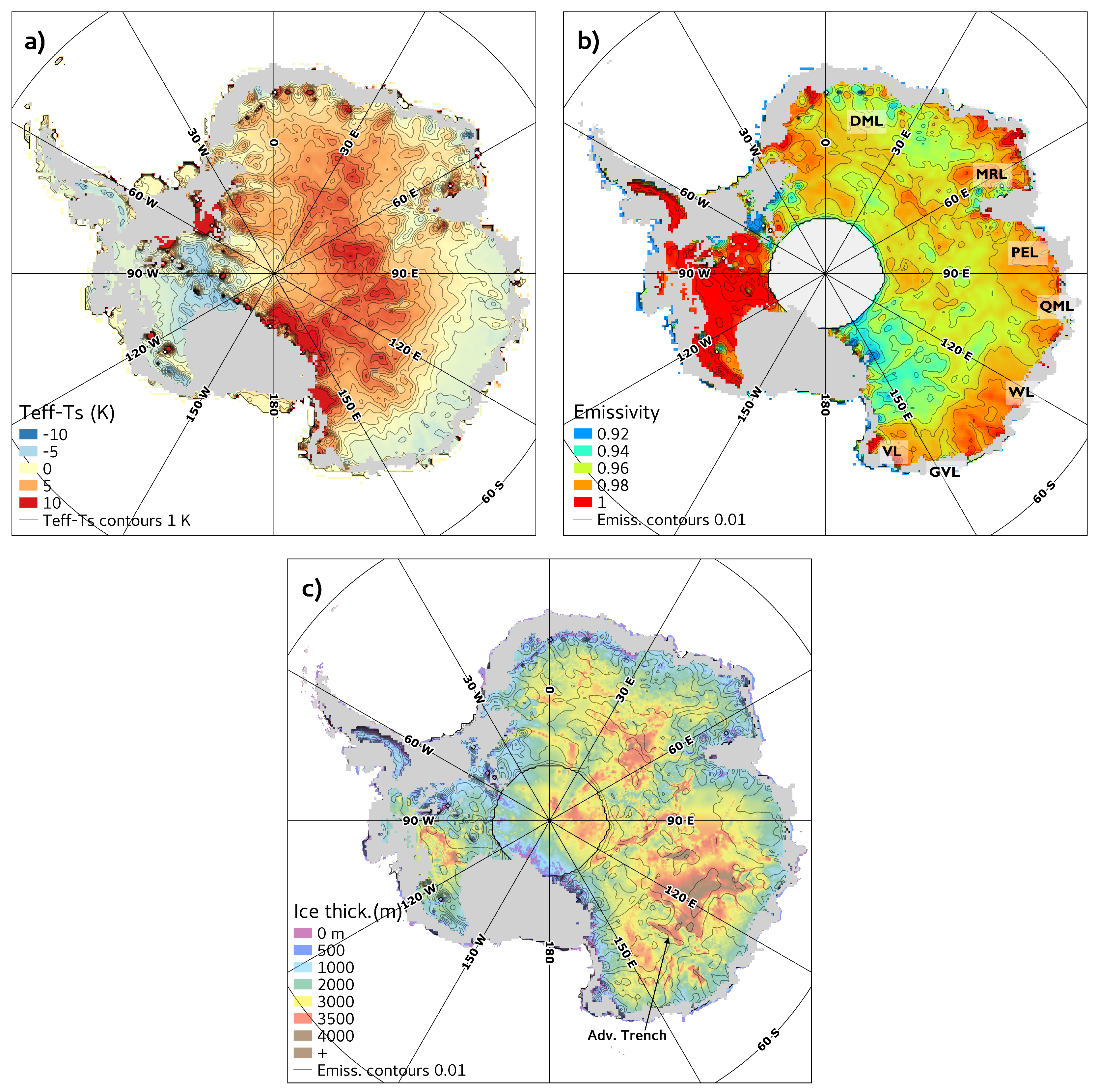
3.4. Effective Temperature and Emissivity

The Mätzler model being validated, it is combined to the expression of $T_E$ in Equation (2) to compute effective temperatures over the whole continent. This approach (Hypothesis 2) is slightly more accurate than using the best estimates of the absorption coefficient, but the results are overall similar. Figure 6a shows the difference between $T_E$ and $T_s$ (‘$T_E$−$T_s$’), and highlights the influence of ice thickness on $T_E$ estimates. The resulting field shows two distinct regions. Areas where $T_E-T_s$ is positive (in red) are located inland where the thermal diffusion is dominant with respect to horizontal and vertical advection. Temperature gradient is mainly driven by ice thickness, which explains why features of the bedrock are visible in this map, at least where basal ice is temperate. For example, the deep topography at Lake Vostok is marked by a $-3$ K anomaly in $T_E$ compared to its surroundings. On the contrary, where $T_E-T_s$ is negative (in blue), thermal advection is significant, affecting the shape of the temperature profiles and reducing the influence of ice thickness. In West Antarctica and near the coast in East Antarctica, bedrock features are not visible in the spatial variations of $T_E-T_s$.

Emissivities are computed from Equation (1) and this estimation of $T_E$. The main part of grounded West Antarctica showed very high emissivity values, between 0.99 and 1 (Figure 6b). In certain parts of Marie Byrd Land in West Antarctica, and in the Antarctic peninsula, emissivity estimates may exceed 1, but by a very small amount ($1<\eta <1.005$). These unphysical values are probably due to the precision of the input temperature field. Over the Antarctic plateau, emissivity generally ranges between $0.96$ and $0.98$, for example, in Wilkes land (WL), Queen Mary land (QML), Princess Elizabeth land (PEL), and Dronning Maud land (DML). However, several large patterns of lower emissivity ($0.94<\eta <0.96$, green) appeared, in particular in George V land (GVL), WL (lon∼110${}^{°}$ E) and eastern DML. Patterns of high emissivity ($>0.99$) arise in MacRobertson Land (MRL) and Victoria land (VL).

According to our assumption of independence between the emissitivity and absorption used in the retrieval method, emissivity is expected to have small dependence on ice thickness. Contour lines of emissivity in Figure 6b were reported on the ice thickness map in Figure 6c. Most of the emissivity contour lines appeared unrelated to ice-thickness patterns, for example, in GVL, MRL, and DML, or in West Antartica. Lake Vostok is crossed by the contour lines and not confined in them. However, this is not the case everywhere; several emissivity contours follow ice-thickness variations as at Adventure Trench, east of Dome C (Figure 5c), the color pattern describing that the deep ice thickness around this site (above 4000 m) is associated to emissivity contour lines. Either this is an artefact coming from a misrepresentation of the temperature field by GRISLI—for example, due to erroneous geothermal flux, or an overestimated advection that leads to an underestimation of $T_E$—or this effect is real, and highlights the influence of bed topography on surface physical mechanisms. Basal ice surely reaches the melting point in such a trench, and a misestimation of advection would affect the surroundings as well, so the first hypothesis is not favored at this stage. Thereby, independence between emissivity and effective temperature may not be complete everywhere.

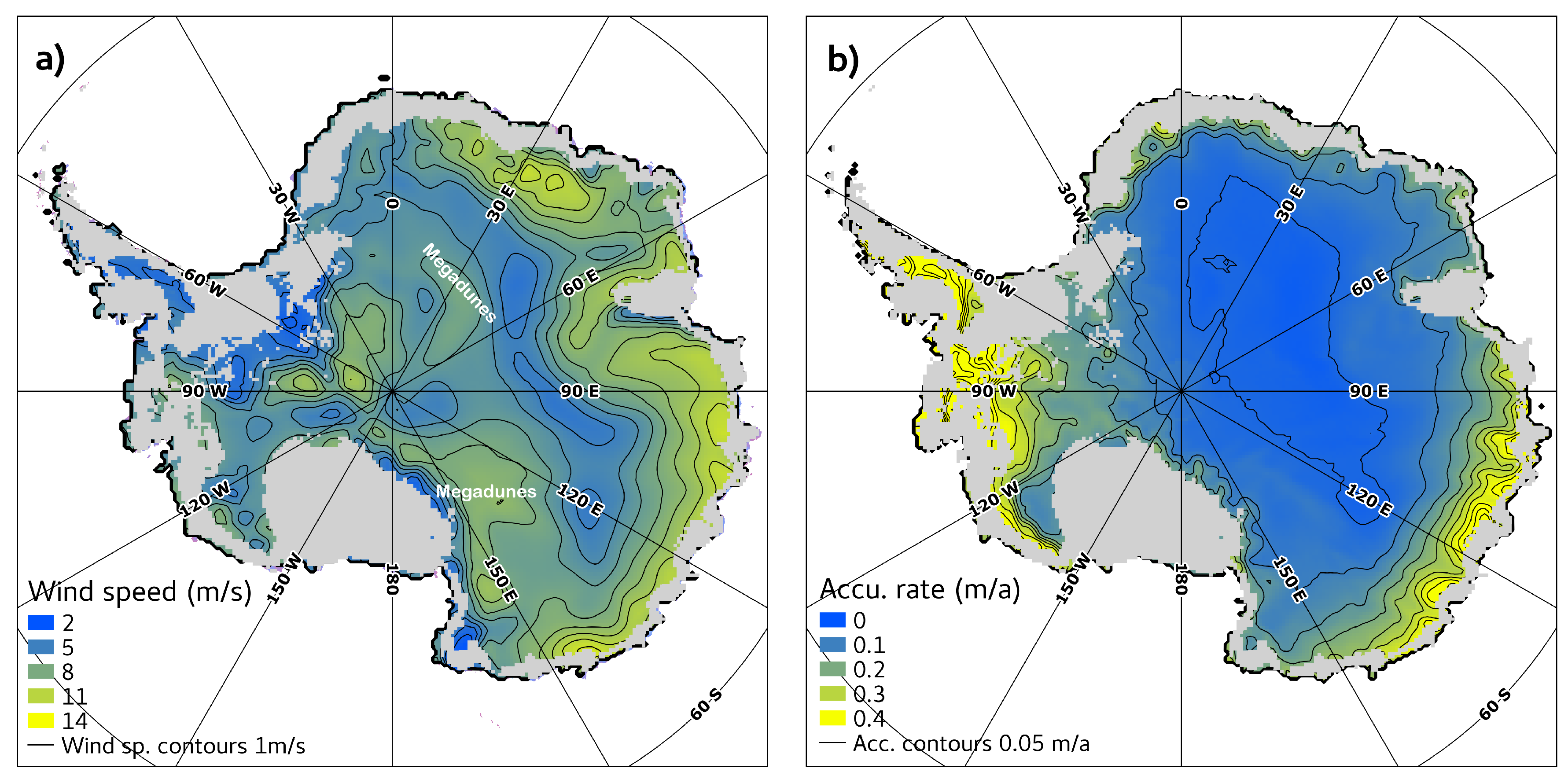
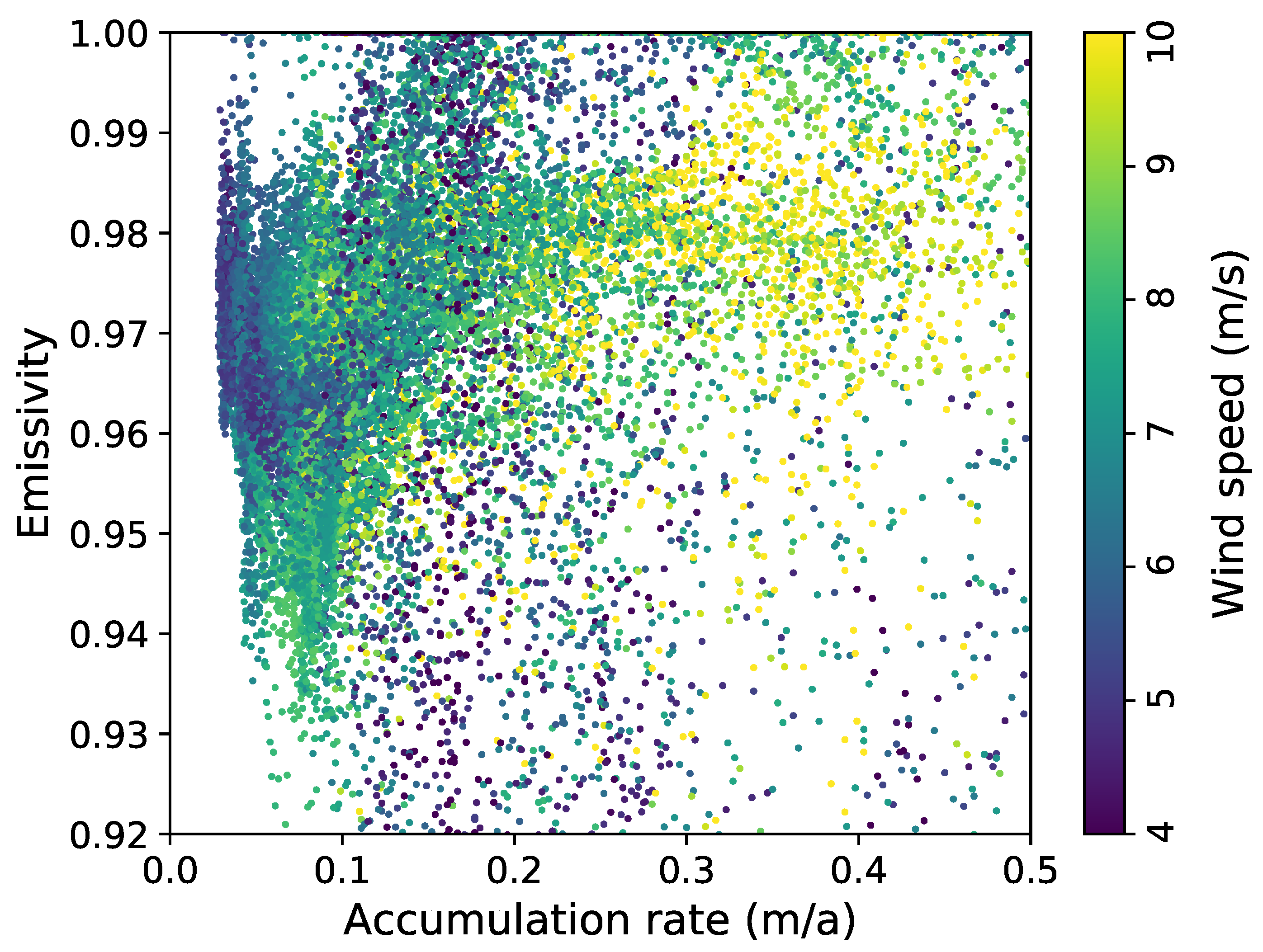
3.5. Relationship between Emissivity, Wind, and Accumulation Fields

To understand the reason for emissivity spatial variations, and potentially reveal the source of scattering, the relationship to climatic parameters is explored. Wind speed at 10 m shown in Figure 7a was extracted from the ERA Interim reanalysis [46], and averaged at each point over the 1980–2016 time period. Several regions of East Antarctica show similar patterns between wind speed and emissivity. Two regions of megadune fields (east of Dome C and south of Dome Fuji) and eastern DML correspond to strong winds and low emissivities. Conversely, low values of wind speed in MRL, VL and western DML correspond to high emissivity values. No pattern emerges in West Antarctica, where emissivity appears uniform.

However, wind speed does not fully explain emissivity variations, as, for instance, both eastern DML and WL undergo similar high wind speed, while the latter has emissivity 2% higher than the former. This may be explained by the difference of accumulation rate, which is up to three times higher on coastal WL than on DML (Figure 7a [4]). High emissivities in West Antarctica correspond to a high accumulation rate as well. Thus, accumulation appears to have two possible opposite effects on brightness temperature: first, emissivity increases with the accumulation rate (for regions with similar wind speeds), and second, accumulation increases horizontal and vertical advection, which cools the ice column. The effect of high advection cooling yields a 500 km-wide band of negative $T_E-Ts$ values in WL (Figure 6a), as $T_E-Ts$ remains positive in eastern DML where advection is smaller.

The joint distribution of accumulation rate and emissivity is plotted in Figure 8. Each dot, representing a 25 km $\times 25$ km pixel, is colored as a function of the wind speed. The shape of the cloud of points suggests that high accumulation rates favor high emissivities (sparse cloud below $\eta =0.97$ for accumulations higher than 0.25 m a${}^{-1}$, dense cloud above). Accumulation at least higher than 0.15 m a${}^{-1}$ are required to have emissivities values higher than 0.99. For emissivity equal to 0.98, a regular wind gradient with accumulation is visible. This means that a given emissivity may either be the result of a low accumulation and low wind, or high acumulation and high wind.

4. Discussion

The explicit assumption underlying this work is that emissivity and effective temperature are not controlled by the same mechanisms, making appropriate disaggregation possible. The method generally succeeds in ascribing glaciological mechanisms (ice-thickness patterns) to $T_E$, and surface-climate mechanisms (e.g., wind patterns) to $\eta$. In particular, the appearance of wind patterns in emissivity variations is a remarkable point, since no wind information is given as input in the retrieval, and similar patterns are barely visible in $T_B$. However, this assumption does not apply to all the players, for instance, accumulation is a surface mechanism that influences the whole ice column, acting on both emissivity and effective temperature. This could yield a remaining statistical dependence between $T_E$ and $\eta$. Nevertheless, this dependence is limited where accumulation has few variations for a given temperature slice, which is the case on the Antarctic plateau (Figure 1b and Figure 7b).

A key result of this study is that the high absorption of the Tiuri model is incompatible with SMOS observations. Despite the few assumptions and the remaining correlation that represent limitations, it is possible to rule out this model with confidence. Ice certainly has lower absorptions. However, given these limitations, it is difficult to assess whether the excellent fit with the Mätzler model was obtained by chance or not. Note that using a more complex electromagnetic model than the approximation in Equation (4), or a better ice temperature field, would certainly provide more accurate $T_E$, but would not radically affect the respective magnitudes of $\mathcal{R}$ between Tiuri and Mätzler. Among our three initial hypotheses, the second one is the most appropriate by far, highlighting that the origin of emissivity variations must be examined.

Our results naturally yield a few worthwhile considerations concerning the mechanisms that influence reflectivity within the firn. First, unlike Macelloni et al. (2016) [10], we did not account for density variations between the layers that leads to contrasts increasing reflectivity at the interfaces, which was justified by the use of observations at vertical polarisation and close to the Brewster angle. However, the Brewster angle depends on the real part of permittivity, which is driven by density in snow and firn. This fundamentally hampers obtaining observations entirely free of internal reflections. As a consequence, the brightness temperature may have a slight dependence on the density variability of firn layers, even close to the Brewster angle. Previous modelling results suggested this dependence may reach 5 K or more at 55${}^{°}$, corresponding to 2% of emissivity [34]. Second, the presence of wind patterns in the emissivity field could be a signature of the roughness of buried layers, that would cause surface scattering at each interlayer interface. Indeed, if the interface is not locally horizontal, the wave hits the interface with an incidence angle different from the Brewster angle, which increases internal reflections within the firn. As the wavelength is 21 cm, decimeter-high or long features are good candidates, such as buried sastrugi [56]. This angular dependence of the $T_B$ signal could lead to a decrease of ∼5 K, corresponding to a 2%-lower emissivity. As an illustration, megadune fields [57] are known to be favorable to the formation of sastrugi (strong and permanent wind, alternance of erosion/deposition areas), including possible severe sastrugi of 1.5 m high [58]. The two main megadune fields reported by Fahnestock et al. (2000) [57] (Figure 7a) correspond to low anomalies of our emissivity field compared to their surroundings ($-1$% near Dome Fuji, and between $-1$% and $-2$% near Dome C). The accumulation seems to be the second parameter influencing emissivity. A possible mechanism involves the fact that regular supply of fresh snow on forming sastrugi tends to moderate erosion and metamorphism [29], and limits their size or hardness. It, thus, decreases the permittivity contrast between the layers, and reduces the amplitude of buried sastrugi.

5. Conclusions

We presented a method to disaggregate the brightness temperature signal at L-band and vertical polarization with an incidence angle close to the Brewser angle, so that the absorption and scattering processes are disentangled. The retrieval algorithm yielded the optimal value of the absorption coefficient that minimizes the statistical dependence between emissivity and effective temperature. The inferred values appeared to be much closer to the permittivity model proposed by Mätzler et al. (2006) [38] than to the one of Tiuri et al. (1984) [36]. This important result meets the objective of this study. In addition, the method gives spatial variations of emissivity over the Antarctic. It shows that emissivity is lower than 1 and highlights significant spatial variations, up to 6%, which are generally independent from ice thickness. These variations seem to be related in both wind speed and accumulation rate at the surface. Wind systematically decreases emissivity (and so $T_B$), whereas the effect of accumulation influences both emissivity and ice temperature, with opposite effects on $T_B$. The fact that emissivity was not close to 1 at vertical polarization and at the Brewster angle was due to scattering effects. Grain size was excluded to have a significant effect at the L-band. Possible sources include density fluctuation in the firn due to stratification, and buried sastrugi that affect the reflectivity of the microwave signal at the layer interface in the firn. Further efforts will have to quantify these effects and check these hypotheses.

This study took place within a more general framework, with glaciological aims, where estimating ice temperature is the ultimate target. For practical reasons, we led this preliminary step where temperature was considered as a known variable. The number of unknown variables in the disaggregation of $T_B$ is now reduced since the Mätzler permittivity model can be considered as suitable. Where emissivity is close to 1, ice-temperature retrieval could be designed in order to obtain constraints on the temperature profiles, and thus learn more about the geothermal flux at bedrock level. This is the case in the central part of the West Antarctic ice sheet (Marie Byrd Land), and in the peninsula. However, where emissivity differs from 1 and has significant and unexplained variations, obtaining constraints on $T(z)$ using the same $T_B$ dataset and our emissivity product is a circular problem. Symmetrically, retrieving emissivity and effective temperature everywhere is an underconstrained problem. An approach using observation at multiple low frequencies is an important avenue for future work.

References

1. Chang, T.; Gloersen, P.; Schmugge, T.; Wilheit, T.; Zwally, H. Microwave emission from snow and glacier ice. J. Glaciol. 1976, 16, 23–39. [Google Scholar] [CrossRef]
2. Brucker, L.; Picard, G.; Fily, M. Snow grain-size profiles deduced from microwave snow emissivities in Antarctica. J. Glaciol. 2010, 56, 514–526. [Google Scholar] [CrossRef]
3. Rotman, S.; Fisher, A.; Staelin, D. Inversion for physical characteristics of snow using passive radiometric observations. J. Glaciol. 1982, 28, 179–185. [Google Scholar] [CrossRef]
4. Arthern, R.J.; Winebrenner, D.P.; Vaughan, D.G. Antarctic snow accumulation mapped using polarization of 4.3-cm wavelength microwave emission. J. Geophys. Res. 2006, 111. [Google Scholar] [CrossRef] [Green Version]
5. Zwally, H.J.; Gloersen, P. Passive microwave images of the polar regions and research applications. Polar Rec. 1977, 18, 431–450. [Google Scholar] [CrossRef]
6. Schneider, D.P.; Steig, E.J.; Comiso, J.C. Recent climate variability in Antarctica from satellite-derived temperature data. J. Clim. 2004, 17, 1569–1583. [Google Scholar] [CrossRef]
7. Zwally, H.J.; Fiegles, S. Extent and duration of Antarctic surface melting. J. Glaciol. 1994, 40, 463–475. [Google Scholar] [CrossRef] [Green Version]
8. Torinesi, O.; Fily, M.; Genthon, C. Interannual variability and trend of the Antarctic summer melting period from 20 years of spaceborne microwave data. J. Clim. 2003, 16, 1047–1060. [Google Scholar] [CrossRef]
9. Picard, G.; Fily, M. Surface melting observations in Antarctica by microwave radiometers: Correcting 26-year time series from changes in acquisition hours. Remote Sens. Environ. 2006, 104, 325–336. [Google Scholar] [CrossRef]
10. Macelloni, G.; Ritz, C.; Picard, G.; Brogioni, M.; Leduc-Leballeur, M. Analyzing and modeling the SMOS spatial variations in the East Antarctic Plateau. Remote Sens. Environ. 2016. [Google Scholar] [CrossRef]
11. Hooke, R. Flow law for polycrystalline ice in glaciers’ comparison of theoretical predictions, laboratory data, and field. Rev. Geophys. Space Phys. 1981, 19, 664–672. [Google Scholar] [CrossRef]
12. Zwally, H.J.; Abdalati, W.; Herring, T.; Larson, K.; Saba, J.; Steffen, K. Surface melt-induced acceleration of Greenland ice-sheet flow. Science 2002, 297, 218–222. [Google Scholar] [CrossRef] [PubMed]
13. Schoof, C. The effect of cavitation on glacier sliding. Proceedings of the Royal Society of London A: Mathematical, Physical and Engineering Sciences. R. Soc. 2005, 461, 609–627. [Google Scholar] [CrossRef]
14. Jouzel, J.; Masson-Delmotte, V. Deep ice cores: The need for going back in time. Quat. Sci. Rev. 2010, 29, 3683–3689. [Google Scholar] [CrossRef]
15. Shapiro, N.M.; Ritzwoller, M.H. Inferring surface heat flux distributions guided by a global seismic model: Particular application to Antarctica. Earth Planet. Sci. Lett. 2004, 223, 213–224. [Google Scholar] [CrossRef]
16. An, M.; Wiens, D.A.; Zhao, Y.; Feng, M.; Nyblade, A.; Kanao, M.; Li, Y.; Maggi, A.; Lévêque, J.J. Temperature, lithosphere-asthenosphere boundary, and heat flux beneath the Antarctic Plate inferred from seismic velocities. J. Geophys. Res. Solid Earth 2015, 120, 8720–8742. [Google Scholar] [CrossRef] [Green Version]
17. Fox Maule, C.; Purucker, M.E.; Olsen, N.; Mosegaard, K. Heat flux anomalies in Antarctica revealed by satellite magnetic data. Science 2005, 309, 464–467. [Google Scholar] [CrossRef] [PubMed]
18. Martos, Y.M.; Catalán, M.; Jordan, T.A.; Golynsky, A.; Golynsky, D.; Eagles, G.; Vaughan, D.G. Heat flux distribution of Antarctica unveiled. Geophys. Res. Lett. 2017, 44, 11–417. [Google Scholar] [CrossRef]
19. Golledge, N.R.; Kowalewski, D.E.; Naish, T.R.; Levy, R.H.; Fogwill, C.J.; Gasson, E.G. The multi-millennial Antarctic commitment to future sea-level rise. Nature 2015, 526, 421. [Google Scholar] [CrossRef]
20. Brucker, L.; Dinnat, E.P.; Picard, G.; Champollion, N. Effect of snow surface metamorphism on Aquarius L-band radiometer observations at Dome C, Antarctica. IEEE Trans. Geosci. Remote Sens. 2014, 52, 7408–7417. [Google Scholar] [CrossRef]
21. Leduc-Leballeur, M.; Picard, G.; Macelloni, G.; Arnaud, L.; Brogioni, M.; Mialon, A.; Kerr, Y. Influence of snow surface properties on L-band brightness temperature at Dome C, Antarctica. Remote Sens. Environ. 2017, 199, 427–436. [Google Scholar] [CrossRef]
22. Drinkwater, M.R.; Floury, N.; Tedesco, M. L-band ice-sheet brightness temperatures at Dome C, Antarctica: spectral emission modelling, temporal stability and impact of the ionosphere. Ann. Glaciol. 2004, 39, 391–396. [Google Scholar] [CrossRef]
23. Pablos, M.; Piles, M.; González-Gambau, V.; Camps, A.; Vall-llossera, M. Ice thickness effects on Aquarius brightness temperatures over Antarctica. J. Geophys. Res. Oceans 2015, 120, 2856–2868. [Google Scholar] [CrossRef] [Green Version]
24. Macelloni, G.; Brogioni, M.; Aksoy, M.; Johnson, J.T.; Jezek, K.C.; Drinkwater, M.R. Understanding SMOS data in Antarctica. In Proceedings of the 2014 IEEE International Geoscience and Remote Sensing Symposium (IGARSS), Quebec City, QC, Canada, 13–18 July 2014; pp. 3606–3609. [Google Scholar] [CrossRef]
25. Van Liefferinge, B.; Pattyn, F. Using ice-flow models to evaluate potential sites of million year-old ice in Antarctica. Clim. Past 2013, 9, 2335–2345. [Google Scholar] [CrossRef] [Green Version]
26. Jezek, K.C.; Johnson, J.T.; Drinkwater, M.R.; Macelloni, G.; Tsang, L.; Aksoy, M.; Durand, M. Radiometric approach for estimating relative changes in intraglacier average temperature. IEEE Trans. Geosci. Remote Sens. 2015, 53, 134–143. [Google Scholar] [CrossRef]
27. Tsang, L.; Kong, J.; Ding, K. Scattering of Electromagnetic Waves, Vol. 1: Theory And Applications; Wieley Interscience: New York, NY, USA, 2000. [Google Scholar]
28. Künzi, K.; Fisher, A.; Staelin, D.; Waters, J. Snow and ice surfaces measured by the Nimbus 5 microwave spectrometer. J. Geophys. Res. 1976, 81, 4965–4980. [Google Scholar] [CrossRef]
29. Picard, G.; Brucker, L.; Fily, M.; Gallée, H.; Krinner, G. Modeling time series of microwave brightness temperature in Antarctica. J. Glaciol. 2009, 55, 537–551. [Google Scholar] [CrossRef]
30. Zwally, H.J. Microwave emissivity and accumulation rate of polar firn. J. Glaciol. 1977, 18, 195–215. [Google Scholar] [CrossRef]
31. Sherjal, I.; Fily, M. Temporal variations of microwave brightness temperatures over Antarctica. Ann. Glaciol. 1994, 20, 19–25. [Google Scholar] [CrossRef] [Green Version]
32. Surdyk, S. Using microwave brightness temperature to detect short-term surface air temperature changes in Antarctica: An analytical approach. Remote Sens. Environ. 2002, 80, 256–271. [Google Scholar] [CrossRef]
33. Mätzler, C. Applications of the interaction of microwaves with the natural snow cover. Remote Sens. Rev. 1987, 2, 259–387. [Google Scholar] [CrossRef]
34. Leduc-Leballeur, M.; Picard, G.; Mialon, A.; Arnaud, L.; Lefebvre, E.; Possenti, P.; Kerr, Y. Modeling L-band brightness temperature at Dome C in Antarctica and comparison with SMOS observations. IEEE Trans. Geosci. Remote Sens. 2015, 53, 4022–4032. [Google Scholar] [CrossRef]
35. Brogioni, M.; Macelloni, G.; Montomoli, F.; Jezek, K.C. Simulating multifrequency ground-based radiometric measurements at Dome C—Antarctica. IEEE J. Sel. Top. Appl. Earth Observ. Remote Sens. 2015, 8, 4405–4417. [Google Scholar] [CrossRef]
36. Tiuri, M.; Sihvola, A.; Nyfors, E.; Hallikaiken, M. The complex dielectric constant of snow at microwave frequencies. IEEE J. Ocean. Eng. 1984, 9, 377–382. [Google Scholar] [CrossRef]
37. Mätzler, C.; Wegmuller, U. Dielectric properties of freshwater ice at microwave frequencies. J. Phys. D Appl. Phys. 1987, 20, 1623. [Google Scholar] [CrossRef]
38. Mätzler, C.; Rosenkranz, P.W.; Battaglia, A.; Wigneron, J.P. Thermal Microwave Radiation: Applications for Remote Sensing; Institute of Engineering and Technology: Stevenage, UK, 2006; Volume 52, Chapter 5; pp. 455–462. [Google Scholar]
39. Picard, G.; Royer, A.; Arnaud, L.; Fily, M. Influence of meter-scale wind-formed features on the variability of the microwave brightness temperature around Dome C in Antarctica. The Cryosphere 2014, 8, 1105–1119. [Google Scholar] [CrossRef] [Green Version]
40. McMullan, K.; Brown, M.A.; Martín-Neira, M.; Rits, W.; Ekholm, S.; Marti, J.; Lemanczyk, J. SMOS: The payload. IEEE Trans. Geosci. Remote Sens. 2008, 46, 594–605. [Google Scholar] [CrossRef]
41. Al Bitar, A.; Mialon, A.; Kerr, Y.H.; Cabot, F.; Richaume, P.; Jacquette, E.; Quesney, A.; Mahmoodi, A.; Tarot, S.; Parrens, M.; et al. The global SMOS Level 3 daily soil moisture and brightness temperature maps. Earth Syst. Sci. Data 2017, 9, 293–315. [Google Scholar] [CrossRef] [Green Version]
42. Brodzik, M.J.; Billingsley, B.; Haran, T.; Raup, B.; Savoie, M.H. EASE-Grid 2.0: Incremental but significant improvements for Earth-gridded data sets. ISPRS Int. J. Geo-Inf. 2012, 1, 32–45. [Google Scholar] [CrossRef]
43. Skoun, N.; Hofman-Bang, D. L-Band radiometers measuring salinity from space: Atmospheric propagation effects. IEEE Trans. Geosci. Remote Sens. 2005, 43, 2210–2217. [Google Scholar] [CrossRef] [Green Version]
44. Quiquet, A.; Dumas, C.; Ritz, C.; Peyaud, V.; Roche, D.M. The GRISLI ice sheet model (version 2.0): Calibration and validation for multi-millennial changes of the Antarctic ice sheet. Geosci. Model Dev. Discuss. 2018, 2018, 1–35. [Google Scholar] [CrossRef]
45. Vionnet, V.; Brun, E.; Morin, S.; Boone, A.; Faroux, S.; Le Moigne, P.; Martin, E.; Willemet, J. The detailed snowpack scheme Crocus and its implementation in SURFEX v7. 2. Geosci. Model Dev. 2012, 5, 773–791. [Google Scholar] [CrossRef] [Green Version]
46. Dee, D.P.; Uppala, S.M.; Simmons, A.; Berrisford, P.; Poli, P.; Kobayashi, S.; Andrae, U.; Balmaseda, M.; Balsamo, G.; Bauer, d.P.; et al. The ERA-Interim reanalysis: Configuration and performance of the data assimilation system. Quart. J. R. Meteorol. Soc. 2011, 137, 553–597. [Google Scholar] [CrossRef]
47. Fréville, H.; Brun, E.; Picard, G.; Tatarinova, N.; Arnaud, L.; Lanconelli, C.; Reijmer, C.; van den Broeke, M. Using MODIS land surface temperatures and the Crocus snow model to understand the warm bias of ERA-Interim reanalyses at the surface in Antarctica. Cryosphere 2014, 8, 1361–1373. [Google Scholar] [CrossRef] [Green Version]
48. Salamatin, A.; Lipenkov, V.Y.; Blinov, K. Vostok (Antarctica) climate record time-scale deduced from the analysis of a borehole-temperature profile. Ann. Glaciol. 1994, 20, 207–214. [Google Scholar] [CrossRef] [Green Version]
49. Tsyganova, E.; Salamatin, A. Non-stationary temperature field simulation along the ice flow line “Ridge B—Vostok Station”, East Antarctica. Mater. Glyatsiol. Issled 2004, 97, 57–70. [Google Scholar]
50. Fujii, Y.; Azuma, N.; Tanaka, Y.; Nakayama, Y.; Kameda, T.; Shinbori, K.; Katagiri, K.; Fujita, S.; Takahashi, A.; Kawada, K.; et al. Deep ice core drilling to 2503 m depth at Dome Fuji, Antarctica. Mem. Natl. Inst. Polar Res. Spec. Issue 2002, 56, 103–116. [Google Scholar]
51. Hondoh, T.; Shoji, H.; Watanabe, O.; Salamatin, A.N.; Lipenkov, V.Y. Depth–age and temperature prediction at Dome Fuji station, East Antarctica. Ann. Glaciol. 2002, 35, 384–390. [Google Scholar] [CrossRef]
52. Gow, A.J.; Ueda, H.T.; Garfield, D.E. Antarctic Ice Sheet: Preliminary Results of First Core Hole to Bedrock. Science 1968, 161, 1011–1013. [Google Scholar] [CrossRef]
53. Dahl-Jensen, D.; Morgan, V.I.; Elcheikh, A. Monte Carlo inverse modelling of the Law Dome (Antarctica) temperature profile. Ann. Glaciol. 1999, 29, 145–150. [Google Scholar] [CrossRef]
54. Wilhelms, F.; Kipfstuhl, S.; Faria, S.; Hamann, I.; Dahl-Jensen, D.; Sheldon, S.; Oerter, H.; Miller, H. Physical properties of ice sheets-implications for, and findings from deep ice core drilling. In Proceedings of the 11th International Conference on the Physics and Chemistry of Ice (PCI-2006), Bremerhaven, Germany, 23–28 July 2006. [Google Scholar]
55. Fretwell, P. Bedmap2: Improved ice bed, surface and thickness datasets for Antarctica. The Cryosphere 2013, 7, 375–393. [Google Scholar] [CrossRef] [Green Version]
56. Rott, H.; Sturm, K.; Miller, H. Active and passive microwave signatures of Antarctic firn by means of field measurements and satellite data. Ann. Glaciol. 1993, 17, 337–343. [Google Scholar] [CrossRef] [Green Version]
57. Fahnestock, M.A.; Scambos, T.A.; Shuman, C.A.; Arthern, R.J.; Winebrenner, D.P.; Kwok, R. Snow megadune fields on the East Antarctic Plateau: Extreme atmosphere-ice interaction. Geophys. Res. Lett. 2000, 27, 3719–3722. [Google Scholar] [CrossRef] [Green Version]
58. Frezzotti, M.; Gandolfi, S.; Urbini, S. Snow megadunes in Antarctica: Sedimentary structure and genesis. J. Geophys. Res. Atmos. 2002, 107. [Google Scholar] [CrossRef] [Green Version]
59. Hooke, R.L. Principles of Glacier Mechanics; Cambridge University Press: Cambridge, UK, 2005. [Google Scholar]
60. Byrd, R.H.; Lu, P.; Nocedal, J.; Zhu, C. A limited memory algorithm for bound constrained optimization. SIAM J. Sci. Comput. 1995, 16, 1190–1208. [Google Scholar] [CrossRef]
61. Zhu, C.; Byrd, R.H.; Lu, P.; Nocedal, J. Algorithm 778: L-BFGS-B: Fortran subroutines for large-scale bound-constrained optimization. ACM Trans. Math. Softw. 1997, 23, 550–560. [Google Scholar] [CrossRef]
Figure 1. (a) Brightness temperature T B measured by the Soil Moisture and Ocean Salinity (SMOS) satellite sensor at the L-band and vertical polarisation, averaged over two years (2013–2014). Black contours are 5 K apart. (b) Surface temperature T s (K) from the Crocus snowpack model. Contour lines are 5 ° C apart and delineate the thermally homogeneous areas used in the retrieval algorithm. Areas undergoing more than five days of melt over the 1979–2007 period are masked in grey and are not accounted for in the study.
Remotesensing 10 01954 g001
Figure 2. Flowchart of the retrieval method developed in the present study.
Remotesensing 10 01954 g002
Figure 3. Borehole temperature profiles at several drilling sites in Antarctica from in situ measurements (solid line) and GRISLI (dashed line). The circles drawn at the surface indicate the value of the SMOS T B for each site (the red point is partly hidden by the blue and green ones.)
Remotesensing 10 01954 g003
Figure 4. Evolution of: (a) the square root of cost function J (K), (b) correlation function R , (c) mean emissivity η ¯ , and (d) e-folding depth 1 / κ a (m) along the iteration steps of the retrieval process. Temperature slice: between 45 and 40 ° C in East Antarctica.
Remotesensing 10 01954 g004
Figure 5. Imaginary part of ice permittivity computed from the Tiuri (orange) and Mätzler (blue) models, depending on ice temperature. The dashed line shows the initial guess of the retrieval process. The result of the retrieval is shown with red (East Antarctica) and green (West Antarctica) diamond markers.
Remotesensing 10 01954 g005
Figure 6. Areas undergoing more than five days of melt over the 1979–2007 time period are masked in grey and were not taken into account in the study. (a) Difference between T E and T s (K). Contour lines are 1 K apart. (b) Emissivity spatial variations as computed from the Mätzler model. DML: Dronning Maud Land, MRL: MacRobertson Land, VL: Victoria Land, GVL: George V Land, PEL: Princess Elizabeth Land, QML: Queen Mary Land, WL: Wilkes Land. Contour lines are 1% apart. (c) Ice thickness (m) from Bedmap 2 [55]. Emissivity contour lines are superimposed.
Remotesensing 10 01954 g006
Figure 7. (a) Average wind speed (m s 1 ) at 10 m from ERA-Interim [46]. Contour lines are 1 m s 1 apart. (b) Accumulation rate at the ice surface from Arthern et al. [4]. Contour lines are 0.05 m y 1 apart.
Remotesensing 10 01954 g007
Figure 8. Scatter plot of emissivity vs. accumulation rate. The color scale correspond to the wind speed of ERA Interim at 10 m.
Remotesensing 10 01954 g008