Snow-Covered Soil Temperature Retrieval in Canadian Arctic Permafrost Areas, Using a Land Surface Scheme Informed with Satellite Remote Sensing Data

Abstract

High-latitude areas are very sensitive to global warming, which has significant impacts on soil temperatures and associated processes governing permafrost evolution. This study aims to improve first-layer soil temperature retrievals during winter. This key surface state variable is strongly affected by snow’s geophysical properties and their associated uncertainties (e.g., thermal conductivity) in land surface climate models. We used infrared MODIS land-surface temperatures (LST) and Advanced Microwave Scanning Radiometer for EOS (AMSR-E) brightness temperatures (Tb) at 10.7 and 18.7 GHz to constrain the Canadian Land Surface Scheme (CLASS), driven by meteorological reanalysis data and coupled with a simple radiative transfer model. The Tb polarization ratio (horizontal/vertical) at 10.7 GHz was selected to improve snowpack density, which is linked to the thermal conductivity representation in the model. Referencing meteorological station soil temperature measurements, we validated the approach at four different sites in the North American tundra over a period of up to 8 years. Results show that the proposed method improves simulations of the soil temperature under snow (Tg) by 64% when using remote sensing (RS) data to constrain the model, compared to model outputs without satellite data information. The root mean square error (RMSE) between measured and simulated Tg under the snow ranges from 1.8 to 3.5 K when using RS data. Improved temporal monitoring of the soil thermal state, along with changes in snow properties, will improve our understanding of the various processes governing soil biological, hydrological, and permafrost evolution.

1. Introduction

The thermal insulation capacity of snow cover, which is well-known, limits winter cooling of underlying soil in Northern regions, thereby influencing the permafrost thermal regime [1]. Permafrost now covers 25% of the landmass of the Northern Hemisphere, and recent studies have shown that about 50% of near-surface permafrost (the top few meters) could thaw by 2050, and 90% by 2100. Sustained by constant warming, this thaw could produce a very significant positive feedback effect (see [2]). Since 70% of northern land areas are covered by snow for more than six months of the year [3], the state of snowpack evolution is one of the key variables governing the evolution of the active layer of permafrost [4,5,6]. Current climate models usually have simple representations of snow (i.e., simplified snow microstructure and density profiles) that lead to erroneous snowpack thermal conductivity [5,7,8,9,10,11]. Moreover, the significant observed shrub expansion in the arctic [12] also modifies snowpack state, which in turn could alter heat transfer mechanisms [6,8,13]. Snowpack thermal conductivity changes under climate warming will affect soil temperatures and permafrost active layer evolution processes, as well as energy and biogeochemical fluxes between land and the atmosphere [14].

Several approaches have been put forward to retrieve soil surface temperatures directly from microwave radiometry, such as those proposed by Holmes et al. [15], Royer and Poirier [16] and Prigent and Rossow [17]; however, none can retrieve soil temperatures under snow. Model-based estimates that include a snow model to better differentiate land surface temperatures (LST) from soil temperatures (Tg) are thus needed to improve retrieval accuracy. Wang et al. [18] reviewed different land surface models (LSM) to retrieve Tg, but they are highly dependent on meteorological driver data, as outlined by Brun et al. [19]. Holmes et al. [20] used microwave observations to retrieve Tg in snow-free conditions only, while Langer et al. [21] proposed satellite-based modeling, combining thermal observations from MODIS and snow data (Globsnow, [22]) to retrieve soil temperature. However, lingering uncertainties remain in the Globsnow dataset, where significant biases were observed in the North (see the discussion in [23]). These important biases in snow mass prediction induce inaccuracies in Tg retrievals. Kohn and Royer [24] previously advanced an approach that uses a complex multilayer physical snow model constrained by microwave brightness temperatures, but which is computationally heavy to implement over large areas.

In this paper, we explore the potential of using satellite-based remote sensing (RS) data to improve the seasonal evolution of the thermal conductivity of the snowpack (snow insulation) in a simple 1-D offline land-surface scheme (the Canadian Land Surface Scheme, or CLASS) [25]. The aim is to improve the soil temperature (Tg) retrievals under snow. We hypothesize that the main uncertainty in the Tg estimates arises from erroneous snowpack microstructure representation in the model, rather than from the soil conductivity parameterization.

2. Materials and Methods

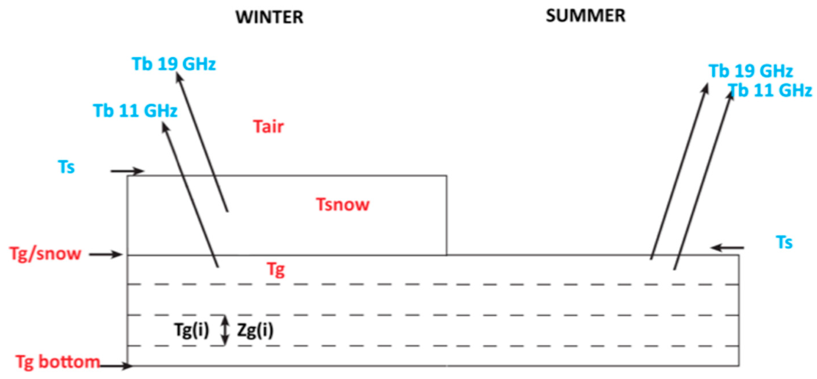
2.1. The Canadian Land Surface Scheme-Specific Surface Area Model

The Canadian Land Surface Scheme (CLASS) 1-D Version 3.5 [25] in an off-line column version was driven by reanalysis of meteorological data [26]. CLASS is used operationally in the Canadian global circulation model [27] and the Canadian Regional Climate Model (CRCM, [28]). CLASS computes the surface energy budget as a function of soil and land-cover types. The standard operational configuration for CLASS consists of three soil layers of 0.10 m, 0.25 m, and 3.75 m in thickness. However, in this study, to allow variations of the deeper layer (3.75 m) and to better account for the effect of phase changes in the soil, the soil was stratified over 47 layers (47 calculation nodes) from 0.1 m to 1.5 m thick, over a total depth of 65 m [29]. In CLASS, the top soil layer is fixed at 0.1 m, which is thicker than the effective soil layer for microwave emission depth [30]. Nevertheless, we assume a correspondence between both layers (see Section 5). CLASS includes prognostic equations for energy and water conservation for the 47 soil layers, while a thermally and hydrologically distinct snowpack is treated as an additional variable-depth layer (see below). In order to represent subgrid-scale variability in a simple manner, CLASS adopts a “pseudo-mosaic” approach and divides the land fraction of a given grid cell into four sub-areas: bare soil, vegetation, snow over bare soil, and snow with vegetation. In this study, for all considered arctic sites, we only used homogeneous grid cells with vegetation corresponding to the grass plant functional type, defined by its structural attributes, including albedo, leaf area index (LAI), roughness length, canopy mass, and rooting depth.

CLASS includes a one-layer snow model described in detail by Bartlett et al. [31] and Brown et al. [32]. The thermal conductivity of snow was calculated from snow density using the empirical relationship described in [33]. However, the CLASS snow model does not simulate the snow grain metamorphism that is needed for the assimilation of passive microwave brightness temperature (Tb). This motivated the implementation of snow grain metamorphism within CLASS by adding an offline snow specific surface area (SSA) model [34]. This offline multilayer model (CLASS-SSA) simulates the decrease of SSA based on snow age, snow temperature, and temperature gradient under dry snow conditions [35], while considering the liquid water content of the snowpack for wet snow metamorphism [36].

The meteorological forcing data were extracted from the National Centers for Environmental Prediction (NCEP) North American Regional Reanalysis (NARR) data [37], and consist of total precipitation mass occurring between two time steps (3 h; kg m⁻²), 2 m air temperature (°C or K) and humidity (%), 10 m wind speed (m s⁻¹), and incoming surface shortwave (SWd) (W m⁻²) and longwave radiation (LWd) (W m⁻²). Meteorological data from the NARR nearest neighbor pixel of each site was used to drive the model. In this study, CLASS-SSA was run at a time step of 30 min, and since NARR provides data for a three-hour time step, all variables were interpolated to a 30-min time step, except precipitation, which was kept on three-hour intervals. A one-year spin-up period was repeated three times, providing three years of spin-up in total, to initialize the model.

2.2. The Helsinki University of Technology Microwave Radiative Transfer Model

Tb was simulated using the one-layer Helsinki University of Technology (HUT) radiative transfer model [38]. The attenuation coefficient of snow was calculated using an empirical equation dependent on the frequency and the effective grain size of the snowpack. The radiative transfer of this simplified one-layer model is based on a two-flux approximation. CLASS-SSA outputs (snow temperature and density and snow grain effective radius derived from simulated SSA and soil temperature) were used as inputs to HUT. The optical radius, calculated from SSA values simulated by CLASS-SSA, was computed to effective grain size (required snow grain input into HUT) by applying a correction factor of 3.7, put forward by Roy et al. [34]. In this study, we only used Tb at 11 and 19 GHz frequencies, given their lower sensitivity to snow grain size scattering (see [39]). Thus, the simplified approach based on CLASS-SSA–HUT models has a small impact on the calculated Tb [34]. When the simulated CLASS soil temperature was below zero, we used soil permittivity values of frozen soil [40], otherwise the soil Dobson permittivities were used [38]. Hereafter, the combined CLASS-SSA models are referred to as CLASS for simplicity.

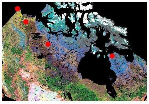
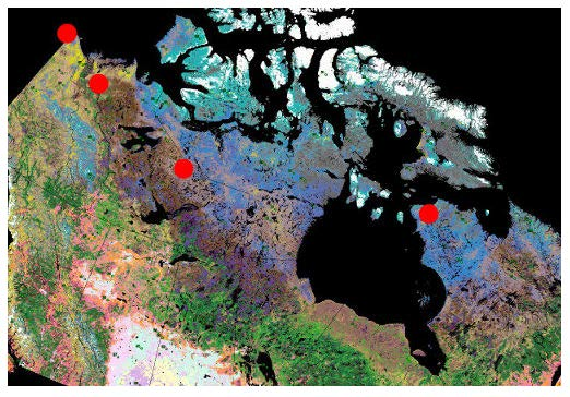
2.3. Reference Study Sites

Four arctic sites where continuous in-situ Tg measurements are available across Canada and the United States were chosen as reference: North Slope, Alaska; Inuvik, Northwest Territories (NWT); Daring Lake, NWT; and Salluit, Nunavik, Québec (Figure 1 and

Table 1. Details of study sites (see Figure 1): mean temperatures (T) (summer: June–August; winter: December–February), total precipitation, and snow water equivalent (SWE).

Sites	Lat., Long., Alt.	Mean Annual T (°C)	Mean Summer T (°C)	Mean Winter T (°C)	Annual Precip. (mm)	Max. SWE (mm)	Period of Analysis
North Slope	70.27N, 148.88W, 15 m	−11	14	−21	330	84.3	October 2007
Inuvik	68.43N, 133.33W, 81 m	−7.2	10	−27	280	115.2	November 2003
Daring Lake	64.52N, 111.54W, 459 m	−6	8	−29	300	136.1	August 2007
Salluit	61.87N, 75.23W, 312 m	−7.8	6	−22	300	236.2	October 2006

). The meteorological characteristics of these sites (provided by Environment and Climate Change Canada) are listed in Table 1. Mean maximum snow water equivalent (SWE) values were derived from the Liston and Hiemstra [3] reconstruction for 1979–2008, showing a significant low-to-high longitudinal gradient from west to east. The percentages of water bodies within the microwave 25 × 25 km² satellite pixel chosen for these sites are (1) North Slope: 2%; (2) Inuvik: 8%: (3) Daring Lake: 10%; and (4) Salluit: 4%. Given its relatively low coverage, the water fraction is assumed to have limited impact on soil temperature retrieval.

2.4. Satellite Data

We used two types of satellite data to constrain the retrieval in this study: microwave Tb from AMSR-E and the thermal infrared LST from AQUA and TERRA MODIS data. The Tb data at 10.7 GHz (“11 GHz”) and 18.7 GHz (“19 GHz”) at the horizontal (H) and vertical (V) polarizations were extracted from the National Snow and Ice Data Center (NSIDC) EASE-Grid 25 × 25 km² product [42]. Both ascendant (13:30) and descendent (01:30) orbits were used. The atmospheric contributions to the satellite Tb were removed by using the millimeter-wave propagation model [43] implemented in the HUT model [38]. The atmospheric model was driven by air temperature and the moisture of the atmospheric layers above the surface from the 29 North American regional reanalysis [37] atmospheric layers.

The MODIS land-surface temperature (LST) data were taken from the NASA 1-km resolution—the daily L3-V6 product (MODIS-Terra MOD11A1 and MODIS-Aqua MYD11A1 Land Surface Temperature products, [44]). This LST product was retrieved from the NASA EOSDIS Land Processes Distributed Active Archive Center (LP DAAC) at the United States Geological Survey (USGS)/Earth Resources Observation and Science (EROS) Center (Sioux Falls, South Dakota, United States). The data is corrected for atmospheric effects and for surface emissivity variation. We resampled the LST data by averaging the LST values at the EASE-Grid 25 km resolution.

3. Inversion Approach

The basic approach used to retrieve Tg was to constrain CLASS simulations with coincident satellite observations. The different temperature variables considered in this study are defined in Figure 2: land surface (skin) temperature (Ts), brightness temperature at 11 and 19 GHz (Tb), and soil temperature (Tg(i) at each layer i). The successive steps for the retrieval procedure are described below (Section 3.1). For the summer period (without snow), we used satellite data to scale CLASS air temperature at 2 m (T_air) and soil moisture simulations by adjusting respectively the summer NARR T_air and precipitation (drivers). For the winter period, we used satellite data to scale CLASS T_air and snow depth by adjusting the winter NARR T_air and precipitation (drivers), respectively. The snow cover density simulations were then adjusted against the Tb polarization ratio at 11 GHz (see Section 3.2).

3.1. Adjustment of Meteorological Driving Data

North American Regional Reanalysis (NARR) meteorological data suffers spatial bias that must be corrected for in local analyses (see [45]). Here, we only adjusted NARR 2-m T_air and the amount of precipitation. Both were corrected by minimizing the root mean square error (RMSE) between the CLASS simulations and the measured satellite-based Ts and Tb. For the summer period, Ts is the surface soil temperature, while for winter, Ts is the snow surface temperature. Also, for summer, Tb is used for fitting the soil moisture, while for winter, it is used for fitting the snow depth—both parameters are governed by precipitation, with T_air > 0 or < 0 °C, respectively.

For the T_air adjustment, we minimized the simulated CLASS Ts against a coincident-measured MODIS LST at four passes (TERRA ascendant (descendant) orbit at 22:30 (10:30) local time; and Aqua ascendant (descendant) orbit at 13:30 (01:30) local time). We adjusted the T_air(h) at each hour (h) using a correcting factor (β_air) such as

$${\mathrm{Tair}}_{\mathrm{corr}}\left(\mathrm{h}\right)={\mathrm{Tair}}_{\max }-{\mathsf{\beta }}_{\mathrm{air}}·\left(1-\cos \frac{\mathsf{\pi }·\left(\mathrm{h}-{\mathrm{t}}_{\max }\right)}{\mathrm{T}}\right)·\left({\mathrm{Tair}}_{\max }-{\mathrm{Tair}}_{\min }\right)$$

(1)

where Tair_corr(h), Tair_max and Tair_min are respectively the corrected, maximum and minimum NARR air temperatures when T = 24 h, and t_max is the time of solar maximum. The factor β_air was optimized by minimizing the RMSE between measured MODIS LST and simulated Ts. Note that the assumption in Equation (1) of sinusoidal behavior about local solar noon could slightly be biased by a possible shift in the daily Tair_max from solar noon by advection, which sometimes occurs at high latitudes and in winter when solar forcing is weak [46]. However, because Tair_corr(h) is then corrected against MODIS observations, such a bias does not significantly impact the results.

Moreover, as the down-welling longwave radiation (LWd) is linked to T_air, we corrected the NARR LWd with the adjusted NARR T_air using a simple linear regression, since LWd_NARR and T_airNARR are well correlated, with R² from 0.5 in summer and 0.82 in winter (not shown). The equation of correction was defined by:

$${\mathrm{LWd}}_{\mathrm{corr}}={\mathrm{LWd}}_{\mathrm{NARR}}-\mathrm{p}\Delta \mathrm{Tair}$$

(2)

where LWd and LWd_NARR are respectively the down-welling longwave radiation corrected and from NARR data; p is the correction factor (i.e., the slope of the regression between LWd_NARR and T_airNARR); and ΔT_air is the difference between T_aircorr and T_airNARR.

For the precipitation amount adjustment, Tb values were simulated at 11 and 19 GHz, using the CLASS outputs as inputs to HUT. For the summer period (T_air > 0 °C), we hypothesize that measured Tb at 11 and 19 GHz are sensitive to the surface soil moisture (SM) [47,48,49], which we assumed to be mainly linked to precipitation. The sensitivity of Tb to SM increases as frequency decreases. The most sensitive AMSR-E bands are thus the X (11 GHz) and Ku (19 GHz) bands. We did not use the C (6 GHz) band, which is contaminated by radio frequency interference, nor the Ka (37 GHz) band, which is known to be less sensitive to SM (higher frequency) and also noisier, because of the vegetation above the soil (see the review [47]). Note that the dual-polarization measurements (Tb H/V), sometimes used for SM products [47], would have probably improved the sensitivity to SM, since the polarization ratio attenuates the physical temperature effects. Figure 3 illustrates the sensitivity of Tb with V of 10.7 and 18.7 GHz to the soil moisture, expressed as %vol. In this example, the non-linear variations are of the order of −1.2 and −0.8 K/% SM, respectively, for 10.7 and 18.7 GHz.

For the winter period, solid precipitation data (deemed to occur when T_air < 0 °C) were adjusted using Tb to correct snow depth. Because of the strong sensitivity of high frequencies (typically 37 GHz or higher) to snow grain size and density (see the review papers from [39,51,52,53,54]), we used both 10.7 and 18.7 GHz channels to optimize the snow depth by adjusting the solid precipitation from the initial NARR values. Figure 4 illustrates typical brightness temperature variations with the snow depth, showing a weak but significant sensitivity of snow depth, with variations of the order of 3 to 4 K/m at 18.7 GHz, and of 3 to 2 K/m at 10.7 GHz (ΔTb/ΔHsnow).

Despite the lower sensitivity of Tb-V 11 and 19 GHz to snow depths, which leads to possible biases in snow depth correction [56], the minimization procedure was carried out using a nonlinear, least-square fitting algorithm to minimize the RMSE between modelled and satellite-based Tb. We thus adjusted the precipitation by a factor Pr_c:

$${\mathrm{Precipitation}}_{\mathrm{corr}}={\mathrm{Pr}}_{\mathrm{c}}{\mathrm{Precipitation}}_{\mathrm{NARR}}$$

(3)

where Pr_c is simply a correcting factor in term of percentage of the initial NARR precipitation amount.

In general, the results of the minimization, with a residual RMSE on Tb 19 V GHz of 2–3 K, lead to a correction factor β_air (Equation (1)) on the order of 0.6–0.75, as well as a reduction of precipitation by 40% to 50% (Pr_c, Equation (3)) [56].

The snowpack insulation effect was corrected in the second processing step (see Section 3.2).

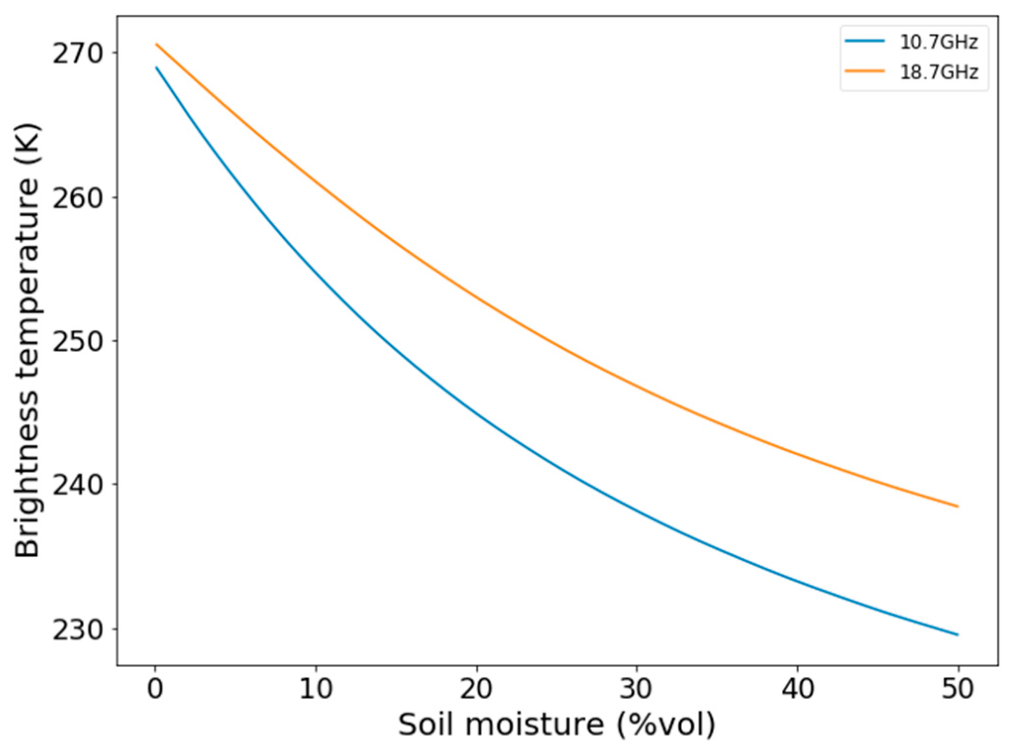
3.2. Snow Density Module Adjustment and Analyzed Variables

The last processing step for retrieving Tg was to constrain the snow density simulated by CLASS using microwave brightness temperature at 11 GHz. The snow density can be linked to the polarization ratio at 11 GHz (PR11 = Tb_11H/Tb_11V) using the same polynomial equation over a large range of snow depths (Figure 5). Assuming that density remains the main uncertainty in the snowpack state (since snow depth and temperature were indirectly adjusted through precipitation and air temperature), this relationship allows the adjustment of the mean snowpack density seasonal evolution using AMSR-E PR11 observations.

Figure 6 shows an example of the daily variations of the measured AMSR-E PR11 compared to simulated PR11 using the outputs of CLASS simulations (snow depth, temperature, and density) for four consecutive winters at the Salluit site (see Figure 1). The observed differences in winter can be attributed to underestimated snow density simulations (red line in Figure 6).

Snow density values from CLASS were adjusted using the observed PR11 in an iterative minimization procedure. We used the Levenberg–Marquardt least squared error minimization algorithm [57], which shows rapid convergence (a maximum of 10 iterations on snow density values to reach a minimum threshold when ΔPR (simulated–measured) is equal to 0.005, corresponding to a variation of snow density of ±20 Kg m⁻³; see example in Figure 7). Using the Sturm et al. [33] relationship between snow effective thermal conductivity (Keff, W m⁻¹ K⁻¹) and density, Keff values were corrected following the derived adjusted snow density values (Figure 7). The new CLASS run, i.e., the snow energy budget and heat transfer within the snowpack with this new value of snow density and the newly derived thermal conductivity, results in a new estimate of the temperature of the first soil layer below the snow.

In summary, the analysis was focused on the simulated variables summarized in

Table 2. Definition of simulated variables used for the analysis.

Variable (See Figure 2)	Acronym	Definition
Surface Temperature	BO Ts	Ts simulated by CLASS, before optimization
	AO Ts	Ts simulated by CLASS, after optimization using RS data (MODIS LST and AMSR-E Tb) (meteorological adjustment)
First layer soil temperature	BO Tg	Tg simulated by CLASS, before optimization
	AO Tg	Tg simulated by CLASS, after optimization using RS data (MODIS LST and AMSR-E Tb) (meteorological adjustment)
	AC Tg	Tg simulated by CLASS, after optimization using RS data (MODIS LST and AMSR-E Tb) and after correction for snow density (using PR 11 GHz)

, and compared to in-situ measurements.

4. Results

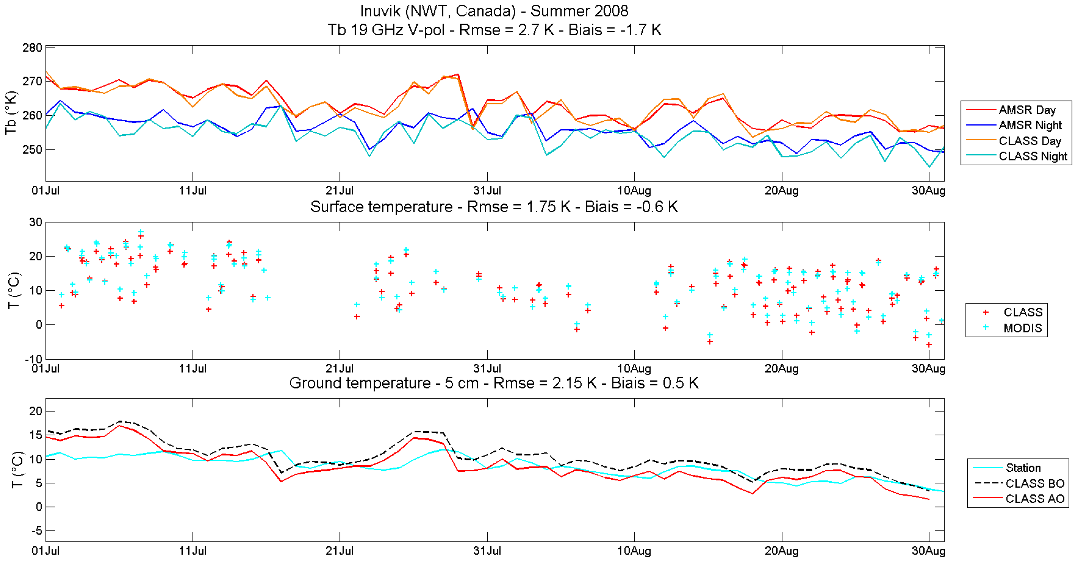
4.1. Summer Soil Temperature Estimates

The summer analysis is used here only to test and calibrate the approach and the efficiency of the simplified T_air and soil moisture adjustment procedure. Results for the Inuvik site are depicted in Figure 8, where a good convergence of the simulated Tb 19 GHz toward the measured Tb (RMSE of 2.7 K and bias of −1.7 K) is observed. Simulations were improved significantly at each site.

Table 3. RMSE and Bias (in K) at the four tundra sites for the available summer time series for the surface temperature (Ts) and soil-temperature (Tg). BO and AO refer respectively to the values before and after optimization procedures (meteorological adjustment) (see definitions in Table 2).

Summer periods (July–August)
Sites	# of Years		BO Ts	AO Ts	BO Tg	AO Tg
Salluit	5	RMSE	5.8	3.4	7.2	3.6
		Bias	2.4	−2.2	3.2	1.9
North Slope	4	RMSE	4.1	2.1	4.3	1.8
		Bias	0.9	−1.4	0.1	−0.2
Inuvik	8	RMSE	5.2	1.9	3.7	2.9
		Bias	1.1	−0.5	1.7	1.4
Daring Lake	2	RMSE	4.1	2.2	9	3
		Bias	−1	−0.7	3.3	1.2
Total	19	RMSE	4.8	2.4	6.1	2.8
		Bias	0.9	−1.2	2.1	1.1

summarizes the results for each studied site over several years. For the 19 summer periods analyzed (four sites and all the years used between 2003 and 2011), results show a reduction by a factor of 2 of the RSME and the bias between measured and simulated Tg, after local adjustment of driving meteorological variables.

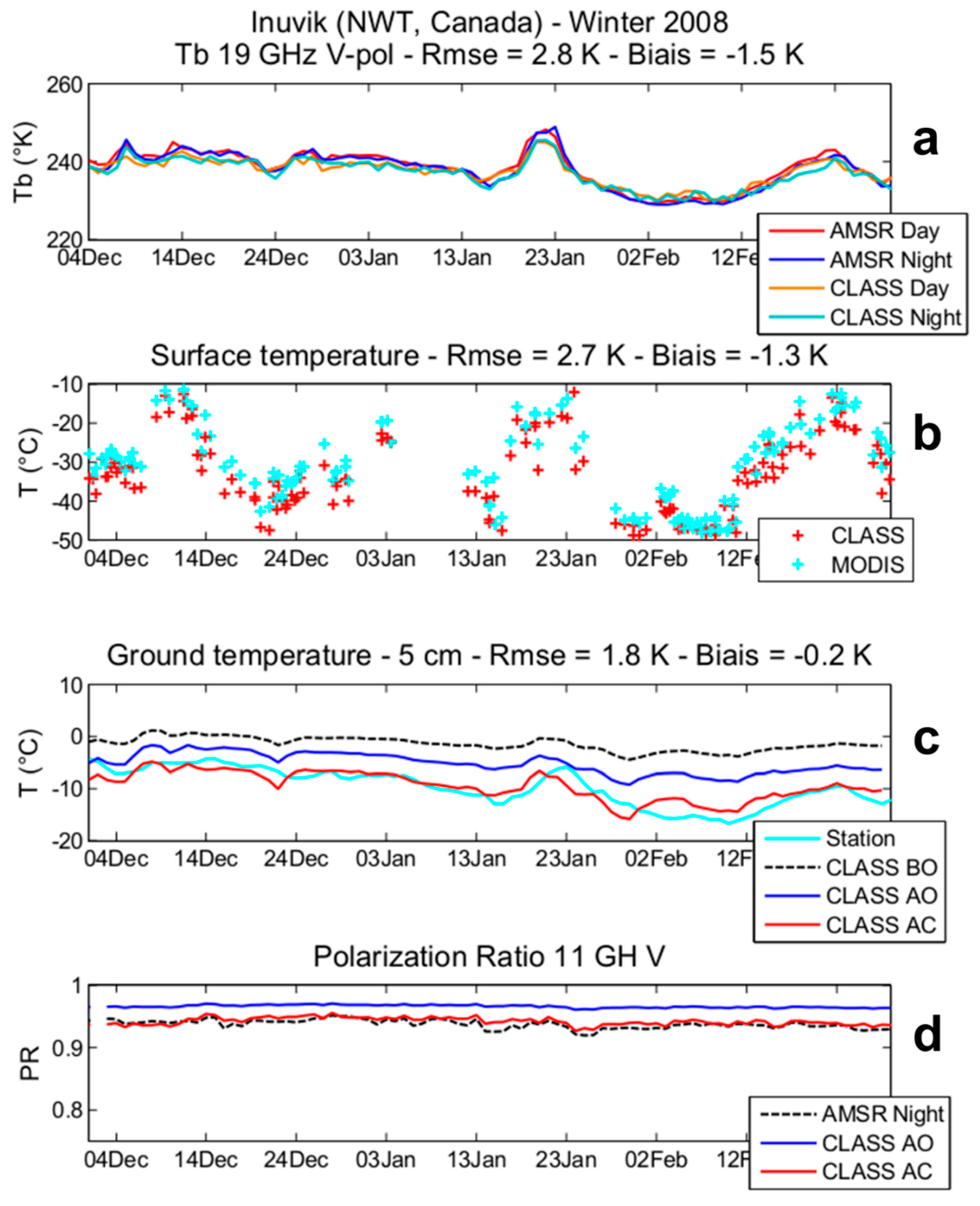
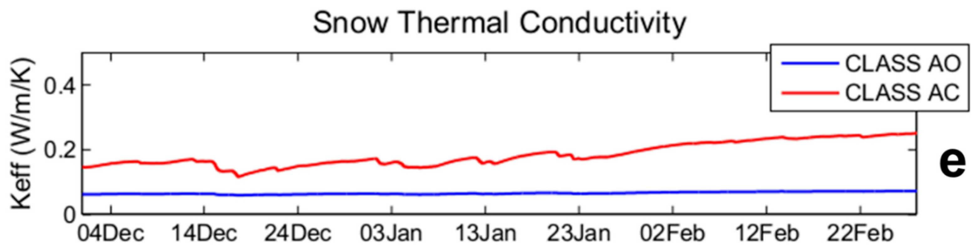
4.2. Snow-Covered Soil Temperature Retrieval in Winter

The winter analysis results for the Inuvik site are highlighted in Figure 9. This example shows the improvement between the raw simulated Tg without RS data—i.e., before the optimization (CLASS BO Tg, the black dotted line in Figure 9c)—compared to the simulated Tg after correcting simulated snow density (CLASS AC Tg, the red line in Figure 9c). Figure 9c clearly shows that the initial simulated soil temperature was too warm, due to an underestimated snow density that led to an overestimation of snow insulation. The adjustment of snow density, using the optimization of simulated PR11 (HUT) with satellite-based measured PR11 (Figure 9d), was able to increase the density and in turn, increase the thermal conductivity (Figure 9e, red line). This higher thermal conductivity reduces the soil temperature under the snow and improves the agreement with soil temperature measurements at the meteorological station.

Table 4. RMSE and bias (in K) at the four tundra sites for the studied winter time series, for the surface temperature (Ts) and soil temperature (Tg). BO refers to the values before the optimization procedure (meteorological adjustment) and AC to the values after correction of the snow density (see definitions in Table 2).

Winter (December–January–February)
Sites	# of Years		BO Ts	AC Ts	BO Tg	AC Tg
Salluit	5	RMSE	7.3	3.5	7.2	3.3
		Bias	1.1	0.2	2.7	0.9
North Slope	4	RMSE	6.8	2.3	7.9	3.1
		Bias	0.7	−1.7	2.3	1.4
Inuvik	8	RMSE	6.8	2.9	7.0	2.0
		Bias	0.8	−1.4	2.2	0.5
Daring Lake	2	RMSE	6.3	1.9	7.7	2.5
		Bias	2.0	−0.4	3.4	0.8
Total	19	RMSE	6.8	2.7	7.5	2.7
		Bias	1.2	−0.8	2.7	0.9

summarizes the results for each studied site, for both the snow surface temperature (Ts), and the snow-covered soil temperature (Tg). The overall results (19 winter periods) show a reduction of 64% in the RSME between the measured and simulated Tg when adjusting with RS data. The mean bias is also significantly reduced from 2.7 K to 0.9 K.

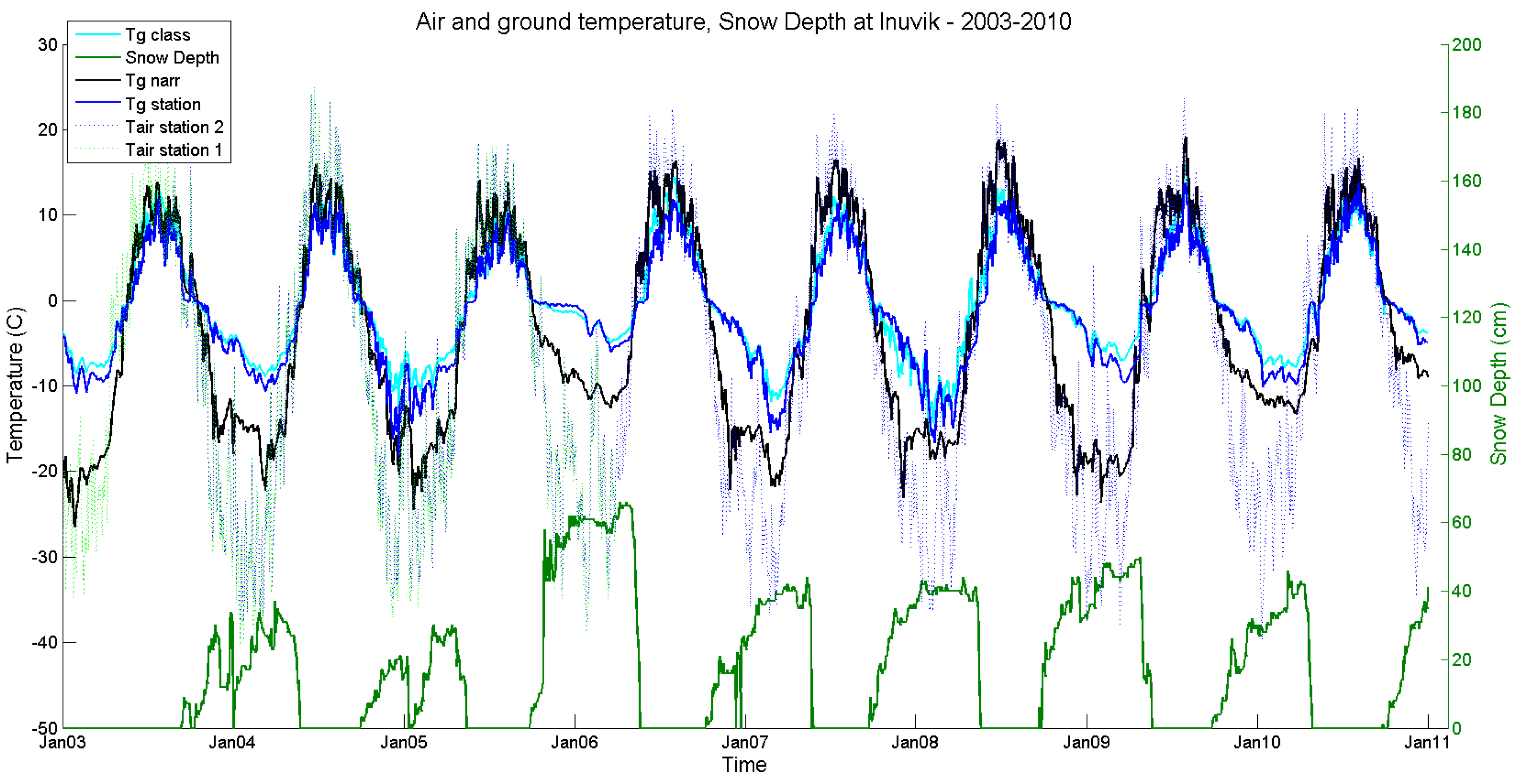
4.3. Time Series Analysis

Figure 10 shows the results of corrected CLASS Tg variations (cyan line) in Inuvik over eight winter periods, compared to in-situ measurements (blue line) and Tg variations derived from NARR data (black line). We show that CLASS-corrected Tg leads to a good representation of soil temperature under the snowpack along the whole period, showing different conditions of temperatures and snow precipitation. In this specific case, Tg values from NARR are too cold, close to Tair, and are probably associated with an underestimated snow insulation effect. It is also suggested that the mean winter Tg is not linked to snow depth in this case (see the discussion from [5]), highlighting the need to better consider the snow insulating effect on Tg. The cumulation of Tg underestimations/overestimations can have significant impacts on the permafrost evolution (see Section 5).

5. Discussion

5.1. Method Limits

The objective of this study was to demonstrate the usefulness of the polarization ratio at 11 GHz to improve simulated snow density through the winter, using a simple one-layer snow model in a climate-model land surface scheme (CLASS, in this case), in order to improve soil temperature retrievals in winter. It is clear that the adjustment methodology used is simple and could be improved with state-of-the-art assimilation schemes (see [58,59,60,61,62,63]). These studies demonstrate possible improvements in snow property retrievals, generally SWE and/or snow depth, using ensemble Kalman or particle filter assimilation schemes. However, despite the simple and computationally light method developed in the present study, we clearly show that the PR11 GHz used with a snow radiative transfer model (HUT) allows constraining snow density and soil temperature under snow in a land surface scheme.

Moreover, the first soil layer in CLASS is fixed at 10 cm, which is substantially thicker than the 11 GHz emission depth (from approximately 5 cm for a dry soil to 0.5 cm for wet soil, [64,65]). The soil temperature values derived from CLASS informed with RS data (AC Tg) should be seen as an effective retrieved temperature. The magnitude of the difference before and after correction (a factor of two; see Table 4) shows that this issue does not invalidate the observed improvements. Future improvements could be made using a heat transfer soil model with a higher vertical resolution near the surface.

One also should note that the proposed approach must be adapted if the surface is covered by vegetation such as shrubs. Vegetation in tundra and taiga zones generates a trapping effect on snow, leading to greater snow depth [66] as well as a modified snowpack state [6,67] that could alter the Tg variations. Because shrub expansion is expected to increase under observed warming [12], the derived snow–vegetation interaction processes should be taken into account in the future in LSM. In addition, for shrubs with a height above the snow cover, vegetation scattering and emission contribution on the microwave signal have to be accounted for in the HUT model using a vegetation radiative transfer model [68].

5.2. Degree-Day Index Comparison

The observed differences between soil temperatures derived from optimized CLASS outputs informed with RS and NARR data, for example, could have a significant impact on permafrost evolution assessment. Figure 11 shows the cumulative effect of winter AC Tg (the frozen degree-day index (FDDI), the sum of negative surface soil temperatures over the year). The values were averaged over the studied period at each site. The NARR-cumulated soil temperatures (FDDI-Ntg, the cross in Figure 11) are significantly underestimated compared to in-situ measurements (FDDI-Stg) and to those retrieved from CLASS (FDDI-Ctg; the proposed approach). The latter is well correlated to in-situ measurements. A significant offset of 1500 to 2000 degree-days appears between these datasets. It is hypothesized that the observed negative bias in temperatures from NARR FDDI is likely a result of underestimated insulating capacity of the snowpack (too-low snow depth or density, for example). These results show that providing RS data to a land surface scheme for improving snow, and in turn soil temperature, could lead to an improved quantification of the evolution of the active layer in permafrost regions.

6. Conclusions

This paper presents a method that uses the polarization ratio from the satellite microwave brightness temperatures at 11 GHz (PR11 H/V) to improve Arctic snow density winter simulations from a simplified snow model in a land surface scheme (LSM) (the CLASS model, in this case). Improved snow density leads to a better estimation of soil temperature under the snow (Tg). Arctic snow has the peculiarity of being very dense near the surface, due to frequent snow-blowing events and sustained cold temperatures, while the bottom of the snowpack is typically less dense, with thick depth hoar layers formed through temperature gradient metamorphism [7]. This leads to a combination of high thermal conductivity for the upper layers and low conductivity for the bottom layers of the snowpack. The result of this combination can significantly alter snowpack-insulating properties, as these layers develop through the winter [67]. No LSM is currently able to accurately simulate such a specific density stratigraphy. The snow models generally produce the reverse density stratigraphy, with low density at the surface and high snow density at the bottom, because they are mostly based on compaction and ignore the water vapor fluxes that lead to depth hoar formation (see [67]). Simulations with CLASS LSM clearly show typical overestimates of soil temperature under the snow. We show that the model can be well corrected by adjusting the mean snow density over the winter (improvement of Tg by a factor of 2) using the PR11 H/V as reference, without the use of any in-situ measurements. In comparison, for the four tundra sites across Canada studied here, the NARR reanalysis dataset shows underestimated (too cold) soil temperatures under the snow, with values close to air temperatures, very likely due to underestimated snowpack insulation.

The examples shown in this paper outline the potential of microwave remote sensing to improve Tg estimates under the snow over the Arctic, which can strongly impact the soil temperature evolution, with significant consequences for permafrost, hydrology (runoff), and soil biochemistry (microbial activities).

References

1. Zhang, T. Influence of the seasonal snow cover on the ground thermal regime: An overview. Rev. Geophys. 2005, 43, RG4002. [Google Scholar] [CrossRef]
2. Chadburn, S.E.; Burke, E.J.; Cox, P.M.; Friedlingstein, P.; Hugelius, G.; Westermann, S. An observation-based constraint on permafrost loss as a function of global warming. Nat. Clim. Chang. 2017, 7, 340–344. [Google Scholar] [CrossRef]
3. Liston, G.E.; Hiemstra, C.A. The changing cryosphere: Pan-Arctic snow trends (1979–2009). J. Clim. 2011, 24, 5691–5712. [Google Scholar] [CrossRef]
4. AMAP. Snow, Water, Ice and Permafrost in the Arctic (SWIPA) 2017; Arctic Monitoring and Assessment Programme (AMAP): Oslo, Norway, 2017; 269p. [Google Scholar]
5. Slater, A.G.; Lawrence, D.M.; Koven, C.D. Process-level model evaluation: A snow and heat transfer metric. Cryosphere 2017, 11, 989–996. [Google Scholar] [CrossRef]
6. Gouttevin, I.; Menegoz, M.; Dominé, F.; Krinner, G.; Koven, C.; Ciais, P.; Tarnocai, C.; Boike, J. How the insulating properties of snow affect soil carbon distribution in the continental pan-arctic area. J. Geophys. Res. Biogeosci. 2012, 117, G02020. [Google Scholar] [CrossRef]
7. Barrere, M.; Domine, F.; Decharme, B.; Morin, S.; Vionnet, V.; Lafaysse, M. Evaluating the performance of coupled snow–soil models in SURFEXv8 to simulate the permafrost thermal regime at a high Arctic site. Geosci. Model Dev. 2017, 10, 3461–3479. [Google Scholar] [CrossRef] [Green Version]
8. Domine, F.; Barrere, M.; Sarrazin, D. Seasonal evolution of the effective thermal conductivity of the snow and the soil in high Arctic herb tundra at Bylot Island, Canada. Cryosphere 2016, 10, 2573–2588. [Google Scholar] [CrossRef]
9. Decharme, B.; Brun, E.; Boone, A.; Delire, C.; Le Moigne, P.; Morin, S. Impacts of snow and organic soils parameterization on northern Eurasian soil temperature profiles simulated by the ISBA land surface model. Cryosphere 2016, 10, 853–877. [Google Scholar] [CrossRef] [Green Version]
10. Chadburn, S.E.; Burke, E.J.; Essery, R.L.H.; Boike, J.; Langer, M.; Heikenfeld, M.; Cox, P.M.; Friedlingstein, P. Impact of model developments on present and future simulations of permafrost in a global land-surface model. Cryosphere 2015, 9, 1505–1521. [Google Scholar] [CrossRef] [Green Version]
11. Lawrence, D.M.; Slater, A.G. The contribution of snow condition trends to future ground climate. Clim. Dyn. 2010, 34, 969–981. [Google Scholar] [CrossRef]
12. Myers-Smith, I.H.; Forbes, B.C.; Wilmking, M.; Hallinger, M.; Lantz, T.; Blok, D.; Tape, K.D.; Macias-Fauria, M.; Sass-Klaassen, U.; Lévesque, E.; et al. Shrub expansion in tundra ecosystems: Dynamics, impacts and research priorities. Environ. Res. Lett. 2011, 6, 045509. [Google Scholar] [CrossRef]
13. Sturm, M.; McFadden, J.; Liston, G.; Chapin, F., III; Racine, C.; Holmgren, J. Snow-shrub interactions in arctic tundra: A hypothesis with climatic implications. J. Clim. 2000, 14, 336–344. [Google Scholar] [CrossRef]
14. Koven, C.D.; Schuur, E.A.G.; Schädel, C.; Bohn, T.; Burke, E.J.; Chen, G.; Chen, X.; Ciais, P.; Grosse, G.; Harden, J.W.; et al. A simplified, data-constrained approach to estimate the permafrost carbon-climate feedback. Philos. Trans. R. Soc. 2015, 373, 20140423. [Google Scholar] [CrossRef] [PubMed]
15. Holmes, T.; De Jeu, R.; Owe, M.; Dolman, A. Land surface temperature from ka band (37 GHz) passive microwave observations. J. Geophys. Res. 2009, 114, D04113. [Google Scholar] [CrossRef]
16. Royer, A.; Poirier, S. Surface temperature spatial and temporal variations in North America from homogenized satellite SMMR-SSM/I microwave measurements and reanalysis for 1979–2008. J. Geophys. Res. 2010, 115, D08110. [Google Scholar] [CrossRef]
17. Prigent, C.; Aires, F.; Rossow, W. Retrieval of surface and atmospheric geophysical variables over snow-covered land from combined microwave and infrared satellite observations. J. Appl. Meteorol. 2003, 42, 368–380. [Google Scholar] [CrossRef]
18. Wang, W.; Rinke, A.; Moore, J.C.; Ji, D.; Cui, X.; Peng, S.; Lawrence, D.M.; McGuire, A.D.; Burke, E.J.; Chen, X.; et al. Evaluation of air–soil temperature relationships simulated by land surface models during winter across the permafrost region. Cryosphere 2016, 10, 1721–1737. [Google Scholar] [CrossRef]
19. Brun, E.; Vionnet, V.; Boone, A.; Decharme, B.; Peings, Y.; Valette, R.; Karbou, F.; Morin, S. Simulation of Northern Eurasian Local Snow Depth, Mass, and Density Using a Detailed Snow- pack Model and Meteorological Reanalyses. J. Hydrometeorol. 2013, 14, 203–219. [Google Scholar] [CrossRef]
20. Holmes, T.R.; Crow, W.T.; Tugrul Yilmaz, M.; Jackson, T.J.; Basara, J.B. Enhancing model-based land surface temperature estimates using multi-platform microwave observations. J. Geophys. Res. Atmos. 2013, 118, 577–591. [Google Scholar] [CrossRef]
21. Langer, M.; Westermann, S.; Heikenfeld, M.; Dorn, W.; Boike, J. Satellite-based modeling of permafrost temperatures in a tundra lowland landscape. Remote Sens. Environ. 2013, 135, 12–24. [Google Scholar] [CrossRef] [Green Version]
22. Takala, M.; Luojus, K.; Pulliainen, J.; Derksen, C.; Lemmetyinen, J.; Kärnä, J.-P.; Koskinen, J.; Bojkov, B. Estimating northern hemisphere snow water equivalent for climate research through assimilation of space-borne radiometer data and ground-based measurements. Remote Sens. Environ. 2011, 115, 3517–3529. [Google Scholar] [CrossRef]
23. Larue, F.; Royer, A.; de Sève, D.; Langlois, A.; Roy, A.; Brucker, L. Validation of GlobSnow-2 snow water equivalent over Eastern Canada. Remote Sens. Environ. 2017, 194, 264–277. [Google Scholar] [CrossRef]
24. Kohn, J.; Royer, A. AMSR-E data inversion for soil temperature estimation under snow cover. Remote Sens. Environ. 2010, 114, 2951–2961. [Google Scholar] [CrossRef]
25. Verseghy, D.L. The Canadian Land Surface Scheme (CLASS): Its history and future. Atmos. Ocean 2000, 38, 1–13. [Google Scholar] [CrossRef]
26. Roy, A.; Picard, G.; Royer, A.; Montpetit, B.; Dupont, F.; Langlois, A.; Derksen, C.; Champollion, N. Brightness temperature simulations of the Canadian seasonal snowpack driven by measurements of snow specific surface area. IEEE Trans. Geosci. Remote. 2013, 51, 4692–4704. [Google Scholar] [CrossRef]
27. Scinocca, J.F.; McFarlane, N.A.; Lazare, M.; Li, J.; Plummer, D. Technical Note: The CCCma third generation AGCM and its extension into the middle atmosphere. Atmos. Chem. Phys. 2008, 8, 7055–7074. [Google Scholar] [CrossRef] [Green Version]
28. Music, B.; Caya, D. Evaluation of the Hydrological Cycle over the Mississippi River Basin as Simulated by the Canadian Regional Climate Model (CRCM). J. Hydrometeorol. 2007, 8, 969–988. [Google Scholar] [CrossRef]
29. Paquin, J.-P.; Sushama, L. On the arctic near-surface permafrost and climate sensitivities to soil and snow model formulations in climate models. Clim. Dyn. 2015, 44, 203–228. [Google Scholar] [CrossRef]
30. Raju, S.; Chanzy, A.; Wigneron, J.-P.; Calvet, J.-C.; Kerr, Y.; Laguerre, L. Soil moisture and temperature profile effects on microwave emission at low frequencies. Remote Sens. Environ. 1995, 54, 85–97. [Google Scholar] [CrossRef]
31. Bartlett, P.A.; MacKay, M.D.; Verseghy, D.L. Modified snow algorithms in the Canadian land surface scheme: Model runs and sensitivity analysis at three boreal forest stands. Atmos. Ocean 2006, 44, 207–222. [Google Scholar] [CrossRef] [Green Version]
32. Brown, R.; Bartlett, P.; MacKay, M.; Verseghy, D. Evaluation of snow cover in CLASS for SnowMIP. Atmos. Ocean 2006, 44, 223–238. [Google Scholar] [CrossRef] [Green Version]
33. Sturm, M.; Holmgren, J.; Konig, M.; Morris, K. The thermal conductivity of seasonal snow. J. Glaciol. 1997, 43, 26–41. [Google Scholar] [CrossRef] [Green Version]
34. Roy, A.; Royer, A.; Montpetit, B.; Bartlett, P.A.; Langlois, A. Snow specific surface area simulation using the one-layer snow model in the Canadian Land Surface scheme (CLASS). Cryosphere 2013, 5, 961–975. [Google Scholar] [CrossRef]
35. Taillandier, A.-S.; Domine, F.; Simpson, W.R.; Sturm, M.; Douglas, T.A. Rate of decrease of the specific surface area of dry snow: Isothermal and temperature gradient conditions. J. Geophys. Res. 2007, 112, F03003. [Google Scholar] [CrossRef]
36. Brun, E. Investigation on wet-snow metamorphism in respect of liquid-water content. Ann. Glaciol. 1989, 13, 22–26. [Google Scholar] [CrossRef]
37. Mesinger, F.; DiMego, G.; Kalnay, E.; Mitchell, K.; Shafran, P.; Ebisuzaki, W.; Jovic, D.; Woollen, J.; Rogers, E.; Berbery, E.; et al. North American regional reanalysis. Bull. Am. Meteorol. Soc. 2006, 87, 343–360. [Google Scholar] [CrossRef]
38. Pulliainen, J.; Grandell, J.; Hallikainen, M. Hut snow emission model and its applicability to snow water equivalent retrieval. IEEE Trans. Geosci. Remote. Sens. 1999, 37, 1378–1390. [Google Scholar] [CrossRef]
39. Matzler, C. Passive microwave signatures of landscapes in winter. Meteorol. Atmos. Phys. 1994, 54, 241–260. [Google Scholar] [CrossRef]
40. Montpetit, B.; Royer, A.; Roy, A.; Langlois, A. In-situ passive microwave parameterization of sub-arctic frozen organic soils. Remote Sens. Environ. 2018, 205, 112–118. [Google Scholar] [CrossRef]
41. Latifovic, R.; Zhu, Z.-L.; Cihlar, J.; Giri, C.; Olthof, I. Landcover mapping of North and Central America—Global land cover 2000. Remote Sens. Environ. 2004, 89, 116–127. [Google Scholar] [CrossRef]
42. Knowles, K.; Savoie, M.; Armstrong, R.; Brodzik, M.J. AMSR-E/Aqua Daily EASE-Grid Brightness Temperatures, Version 1; NASA National Snow and Ice Data Center Distributed Active Archive Center: Boulder, CO, USA, 2006. [CrossRef]
43. Liebe, H. MPM—An atmospheric millimeter-wave propagation model. Int. J. Infrared Millim. Waves 1989, 10, 631–650. [Google Scholar] [CrossRef]
44. Wan, Z.; Hook, S.; Hulley, G. MOD11A1 MODIS/Terra and MYD11A1 MODIS/Aqua Land Surface Temperature/Emissivity Daily L3 Global 1km SIN Grid V006; NASA EOSDIS LP DAAC: Boulder CO, USA, 2015. [CrossRef]
45. Lader, R.; Bhatt, U.S.; Walsh, J.E.; Rupp, T.S.; Bieniek, P.A. Two-Meter Temperature and Precipitation from Atmospheric Reanalysis Evaluated for Alaska. J. Appl. Meteorol. Clim. 2016, 55, 901–922. [Google Scholar] [CrossRef]
46. Wang, A.; Zeng, X. Range of monthly mean hourly land surface air temperature diurnal cycle over high northern latitudes. J. Geophys. Res. Atmos. 2014, 119, 5836–5844. [Google Scholar] [CrossRef] [Green Version]
47. Mladenova, I.E.; Jackson, T.J.; Njoku, E.; Bindlish, R.; Chan, S.; Cosh, M.H.; Holmes, T.R.H.; de Jeu, L.; Kimball, J.K.; Paloscia, S.; et al. Remote monitoring of soil moisture using passive microwave-based techniques—Theoretical basis and overview of selected algorithms for AMSR-E. Remote Sens. Environ. 2014, 144, 197–213. [Google Scholar] [CrossRef]
48. Njoku, E.G.; Jackson, T.J.; Lakshmi, V.; Chan, T.K.; Nghiem, S.V. Soil moisture retrieval from AMSR-E. IEEE Trans. Geosci. Remote. Sens. 2003, 41, 215–229. [Google Scholar] [CrossRef]
49. Ulaby, F.T.; Moore, R.K.; Fung, A.K. Microwave Remote Sensing: Active and Passive: From Theory to Applications; Artech House: Norwood, MA, USA, 1986; Volume III. [Google Scholar]
50. Wegmuller, U.; Matzler, C. Rough bare soil reflectivity model. IEEE Trans. Geosci. Remote. Sens. 1999, 37, 1391–1395. [Google Scholar] [CrossRef]
51. Royer, A.; Roy, A.; Montpetit, B.; Saint-Jean-Rondeau, O.; Picard, G.; Brucker, L.; Langlois, A. Comparison of commonly-used microwave radiative transfer models for snow remote sensing. Remote Sens. Environ. 2017, 190, 247–259. [Google Scholar] [CrossRef]
52. Roy, A.; Royer, A.; St-Jean-Rondeau, O.; Montpetit, B.; Picard, G.; Mavrovic, A.; Marchand, N.; Langlois, A. Microwave snow emission modeling uncertainties in boreal and subarctic environments. Cryosphere 2016, 10, 623–638. [Google Scholar] [CrossRef] [Green Version]
53. Tsang, L.; Ding, K.-H.; Huang, S.; Xu, X. Electromagnetic computation in scattering of electromagnetic waves by random rough surface and dense media in microwave remote sensing of land surfaces. Proc. IEEE TGARS 2013, 101, 255–279. [Google Scholar] [CrossRef]
54. Dietz, A.; Kuenzer, C.; Gessner, U.; Dech, S. Remote sensing of snow—A review of available methods. Int. J. Remote. Sens. 2012, 33, 4094–4134. [Google Scholar] [CrossRef]
55. Picard, G.; Brucker, L.; Roy, A.; Dupont, F.; Fily, M.; Royer, A.; Harlow, C. Simulation of the microwave emission of multilayered snowpacks using the Dense Media Radiative transfer theory: The DMRT-ML model. Geosci. Model Dev. 2013, 6, 1061–1078. [Google Scholar] [CrossRef]
56. Marchand, N. Suivi de la Température de Surface Dans les Zones de Pergélisol Arctique par L’Utilisation de Données de Télédétection Inversées Dans le Schéma de Surface du Modèle Climatique Canadien (CLASS). Ph.D. Thesis, Université de Sherbrooke, Sherbrooke, QC, Canada, 2017; 207p. (In French). [Google Scholar]
57. Marquardt, D. An algorithm for least-squares estimation of nonlinear parameters. J. SIAM Appl. Math. 1963, 11, 431–441. [Google Scholar] [CrossRef]
58. Pietroniro, A.; Leconte, R. A review of Canadian Remote Sensing and Hydrology 1999–2003. Hydrol. Processes. 2005, 19, 285–301. [Google Scholar] [CrossRef]
59. Van Leeuwen, P.J. Particle filtering in geophysical systems. Mon. Weather Rev. 2009, 137, 4089–4114. [Google Scholar] [CrossRef]
60. DeChant, C.; Moradkhani, H. Radiance data assimilation for operational snow and streamflow forecasting. Adv. Water Resour. 2011, 34, 351–364. [Google Scholar] [CrossRef]
61. De Lannoy, G.J.M.; Reichle, R.H.; Arsenault, K.R.; Houser, P.R.; Kumar, S.; Verhoest, N.E.C.; Pauwels, V.R.N. Multiscale assimilation of AMSR-E snow water equivalent and MODIS snow cover fraction observations in northern Colorado. Water Resour. Res. 2012, 48, W01522. [Google Scholar] [CrossRef]
62. Kwon, Y.; Yang, Z.-L.; Hoar, T.J.; Toure, A.M. Improving the Radiance Assimilation Performance in Estimating Snow Water Storage across Snow and Land-Cover Types in North America. J. Hydrometeorol. 2017, 18, 651–668. [Google Scholar] [CrossRef]
63. Larue, F.; Royer, A.; de Sève, D.; Roy, A.; Cosme, E. Assimilation of passive microwave AMSR-2 satellite observations in a snowpack evolution model over North-Eastern Canada. Hydrol. Earth Syst. Sci. 2018. [Google Scholar] [CrossRef]
64. Hallikainen, M.T.; Ulaby, F.T.; Dobson, M.C.; El-Rayes, M.A.; Wu, L.-K. Microwave dielectric behavior of wet soil, Part I: Empirical models and experimental observations from 1.4 to 18 GHz. IEEE Trans. Geosci. Remote Sens. 1985, GE-23, 25–34. [Google Scholar] [CrossRef]
65. Dobson, M.C.; Ulaby, F.T.; Hallikainen, M.T.; El-Rayes, M.A. Microwave dielectric behavior of wet soil-part II: Dielectric mixing models. IEEE Trans. Geosci. Remote. Sens. 1985, GE-23, 35–46. [Google Scholar] [CrossRef]
66. Busseau, B.-C.; Royer, A.; Roy, A.; Langlois, A.; Domine, F. Analysis of snow-vegetation interactions in the low Arctic-Subarctic transition zone (northeastern Canada). Phys. Geogr. 2017, 38, 159–175. [Google Scholar] [CrossRef]
67. Domine, F.; Barrere, M.; Morin, S. The growth of shrubs on high Arctic tundra at Bylot Island: Impact on snow physical properties and permafrost thermal regime. Biogeosciences 2016, 13, 6471–6486. [Google Scholar] [CrossRef]
68. Roy, A.; Royer, A.; Wigneron, J.-P.; Langlois, A.; Bergeron, J.; Cliche, P. A simple parameterization for a boreal forest radiative transfer model at microwave frequencies. Remote Sens. Environ. 2012, 124, 371–383. [Google Scholar] [CrossRef]
Figure 1. Map of study sites. From left (west) to right (east): North Slope, Inuvik, Daring Lake, and Salluit (see Table 1 for description). Base map: land cover map from [41].
Remotesensing 10 01703 g001
Figure 2. Temperatures used in this study for summer (right) and winter (left) periods. Tair is the 2-m air temperature used as a driver (NARR and optimized), Tsnow is the mean snowpack temperature (simulated by CLASS), Tg(i) is the soil temperature simulated by CLASS at each soil layer (i) of thickness Zg(i), Tg/snow is the soil/snow interface temperature (simulated by CLASS), Tg is the first layer soil temperature (simulated by CLASS and measurements for validation), Tg_bottom is the soil temperature of the last soil layer (fixed), Ts is the land surface temperature (MODIS and simulated by CLASS), and Tb is the microwave brightness temperature at 11 and 19 GHz (AMSR-E and simulated by HUT driven with CLASS outputs).
Remotesensing 10 01703 g002
Figure 3. Sensitivity of brightness temperatures (vertical polarization) to soil moisture at 10.7 (blue line) and 18.7 (orange line) GHz (55° viewing angle), based on the [50] rough bare soil reflectivity model (implemented in the HUT model) (soil temperature: 283 K and soil roughness = 0.2 cm).
Remotesensing 10 01703 g003
Figure 4. Sensitivity of brightness temperatures (vertical polarization) to snow depth (m) at 10.7 (blue line) and 18.7 (orange line) GHz for two densities: 200 (continuous lines) and 300 (dotted lines) Kg/m3, based on the model simulations from the Dense Media Radiative Transfer Model (DMRT)_Sticky-Hard-Sphere mode [55] (55° viewing angle, snow temperature = 263 K, snow grain as sticky spheres with optical radius of 0.13 mm and stickiness of 0.2, soil temperature = 273 K; and soil roughness = 0.2 cm).
Remotesensing 10 01703 g004
Figure 5. Theoretical relationship between snow density and the polarization ratio at 11GHz (PR11). The red line is derived from the HUT radiative transfer model, allowing the correction of simulated snow density by CLASS.
Remotesensing 10 01703 g005
Figure 6. Measured polarization ratio PR11 (AMSR-E, in blue) and simulated (HUT, in red) in Salluit from 2005 to 2009 (month/year). A good agreement between simulated and measured PR11 can be observed in summer, while underestimated snow density from CLASS leads to higher PR11 values from HUT in winter.
Remotesensing 10 01703 g006
Figure 7. Convergence of the polarization ratio at 11 GHz (a), the derived snow density variation (b), and the derived simulated snow thermal conductivity (c) at the Salluit site for 2008 and 2009 for winter onset (day 320) and the end of winter (day 112).
Remotesensing 10 01703 g007
Figure 8. Results of air temperature and precipitation optimizations in Inuvik during summer (July and August, day/month) 2008. The top graph shows a comparison between measured (AMSR-E) and adjusted simulated (Canadian Land Surface Scheme (CLASS)) brightness temperatures at 19 V GHz for both orbits. The middle graph shows a comparison between measured (MODIS) and adjusted simulated (CLASS) surface temperatures. The bottom graph shows a comparison between measured (Station), simulated before optimization (CLASS BO), and simulated after optimization (CLASS AO) soil temperatures (Tg).
Remotesensing 10 01703 g008
Figure 9. Results of the adjustment procedure using remote sensing (RS) data at Inuvik for winter 2008 (day/month) for soil temperature retrieval (Tg): (a) 19 GHz Tb comparison of measured (AMSR-E) and simulated (CLASS) at V polarization; (b) measured (MODIS) and simulated (CLASS) surface temperature; (c) measured (Station) soil temperature, simulated before optimization (BO) and after optimization (AO; meteorological adjustments), as well as simulated after snow density corrections (AC); (d) PR11 measured (AMSR-E) and simulated after optimization (AO) and after corrections (AC); and (e) snow thermal conductivity after optimization (AO) and after snow density correction (AC).
Remotesensing 10 01703 g009aRemotesensing 10 01703 g009b
Figure 10. Optimized soil temperature evolution (CLASS AC) compared to the measured data (Station) and NARR simulations, as well as air temperature (Station) and snow depth (Station) in Inuvik during the 2003–2011 period (month/year). The Tair dataset combines data from two nearby meteorological stations to yield a continuous time series (Environment Canada). The overlap period (2004–2005) shows the coherency of both time series.
Remotesensing 10 01703 g010
Figure 11. Mean frozen degree-day index (FDDI) of surface soil temperature (Tg) measured (FDDI-Stg), simulated with NARR (FDDI-Ntg) (cross), and simulated with CLASS (FDDI-Ctg) (square) at the four studied tundra sites (color).
Remotesensing 10 01703 g011