The Benefits of the Ka-Band as Evidenced from the SARAL/AltiKa Altimetric Mission: Scientific Applications

 ,
,  , ,
, ,  , and
, and
Abstract
:
1. Introduction
2. The Ocean
2.1. Observability of the Fine-Scale Ocean Dynamics
2.2. Observability of the Coastal Ocean Dynamics
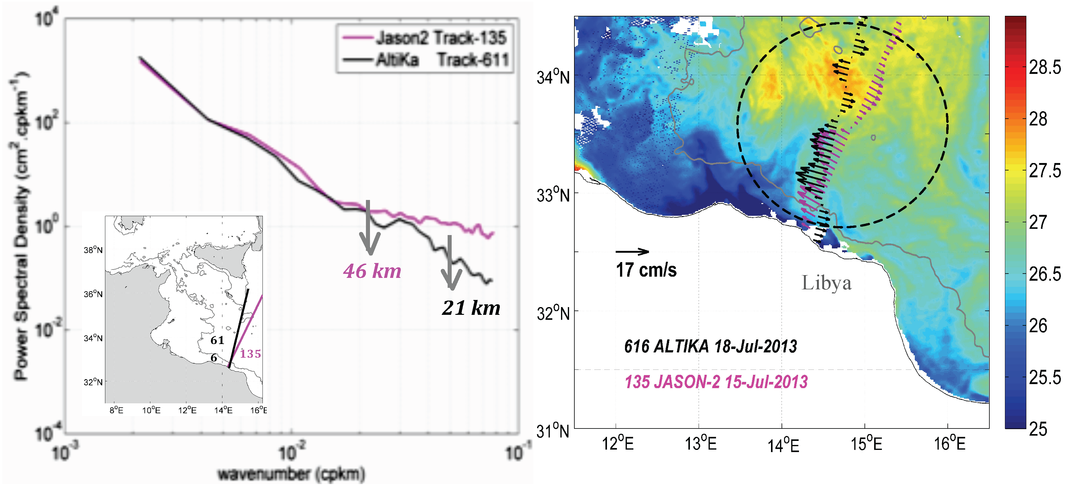
2.2.1. Observability of the Coastal OceanDynamics in the Central Mediterranean Sea
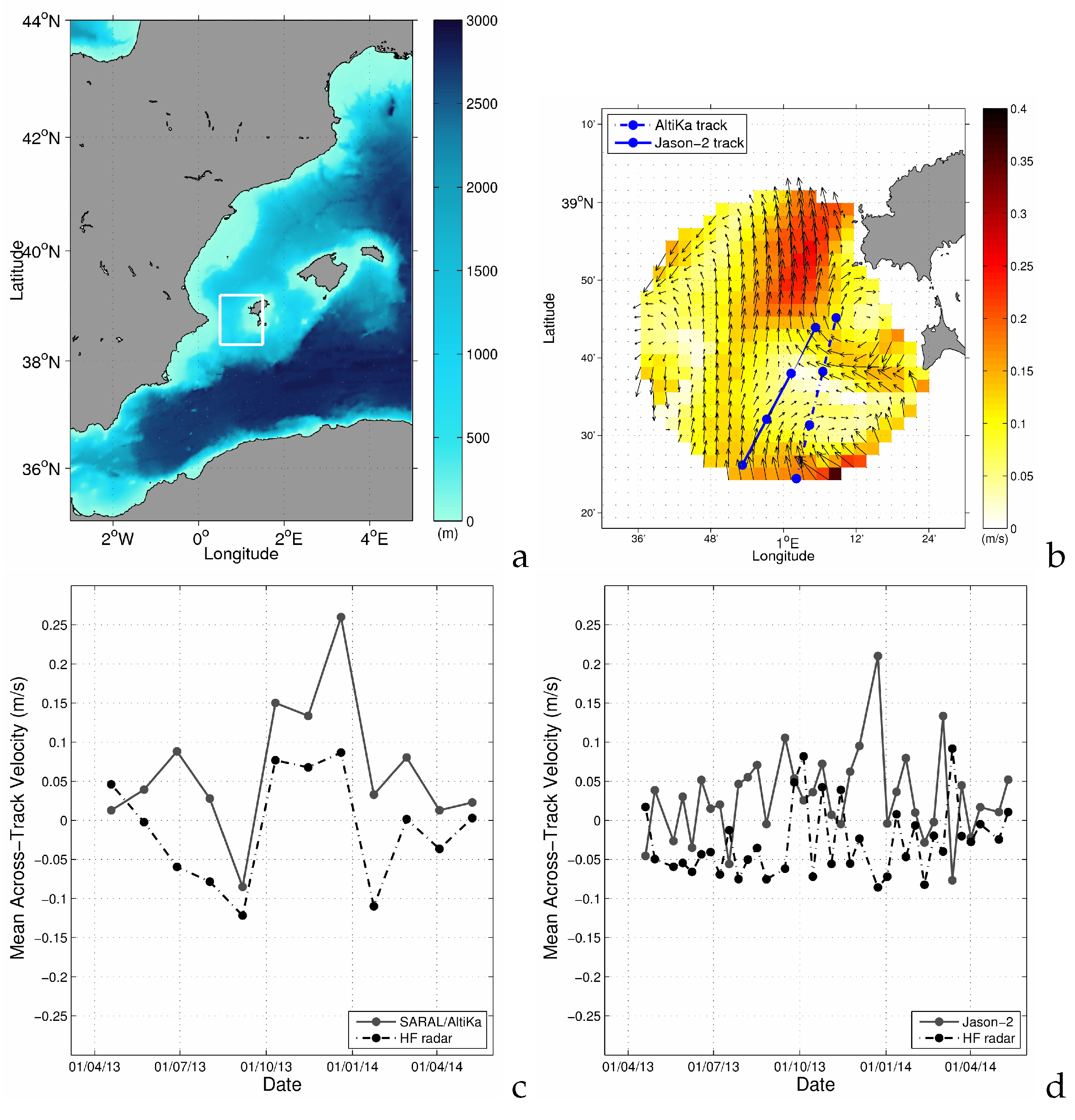
2.2.2. SARAL-AltiKa Capabilities to Detect Coastal Currents: Comparisons With Jason-2 and HF Radar Data
2.3. SARAL/AltiK a Data Into Operational Systems
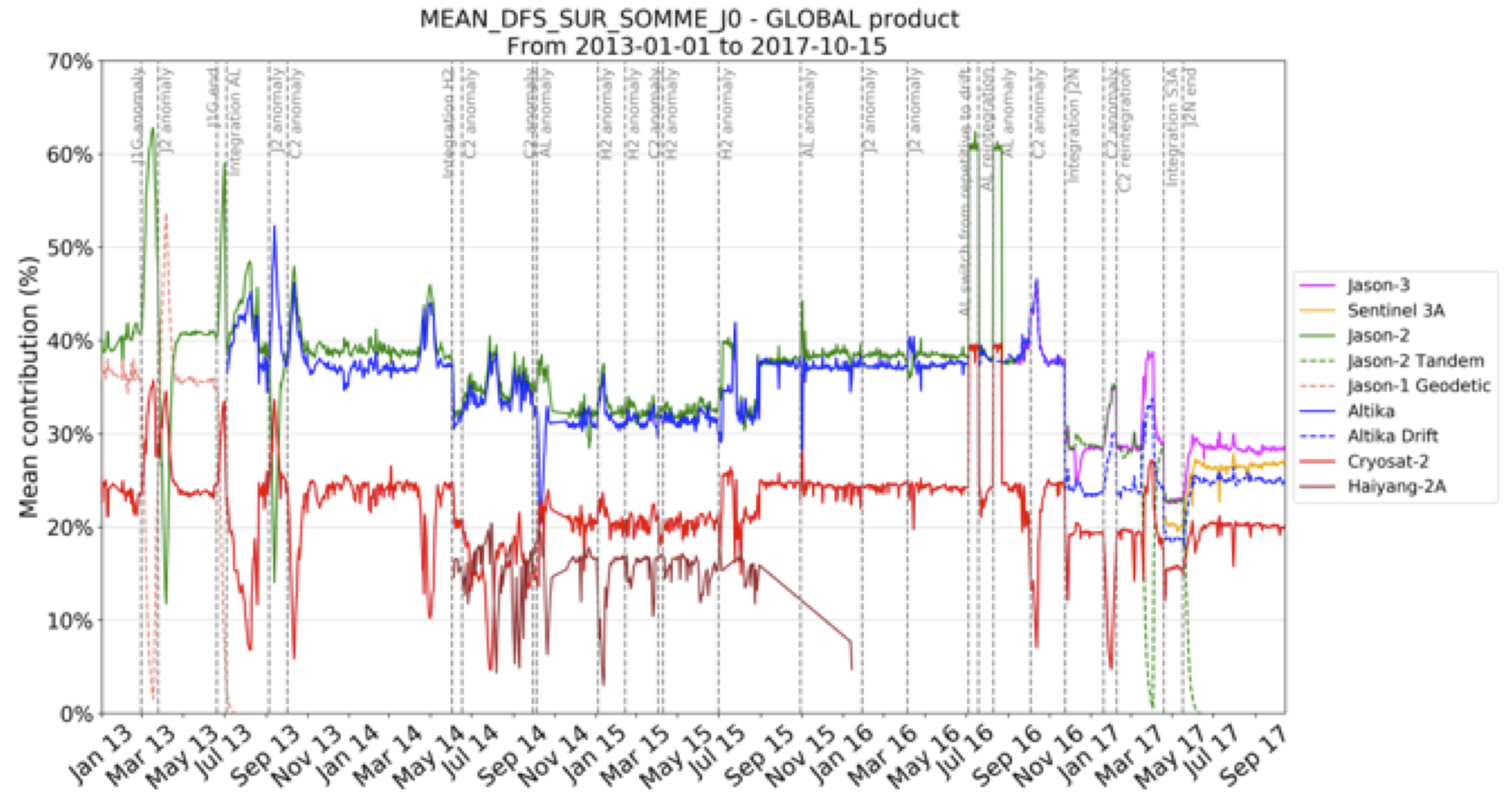
2.3.1. SARAL/AltiK a Major Contributor to DUACS/CMEMS Multi-Mission Seal Level Products
2.3.2. Assimilation of SLA Data in the Mercator Ocean System
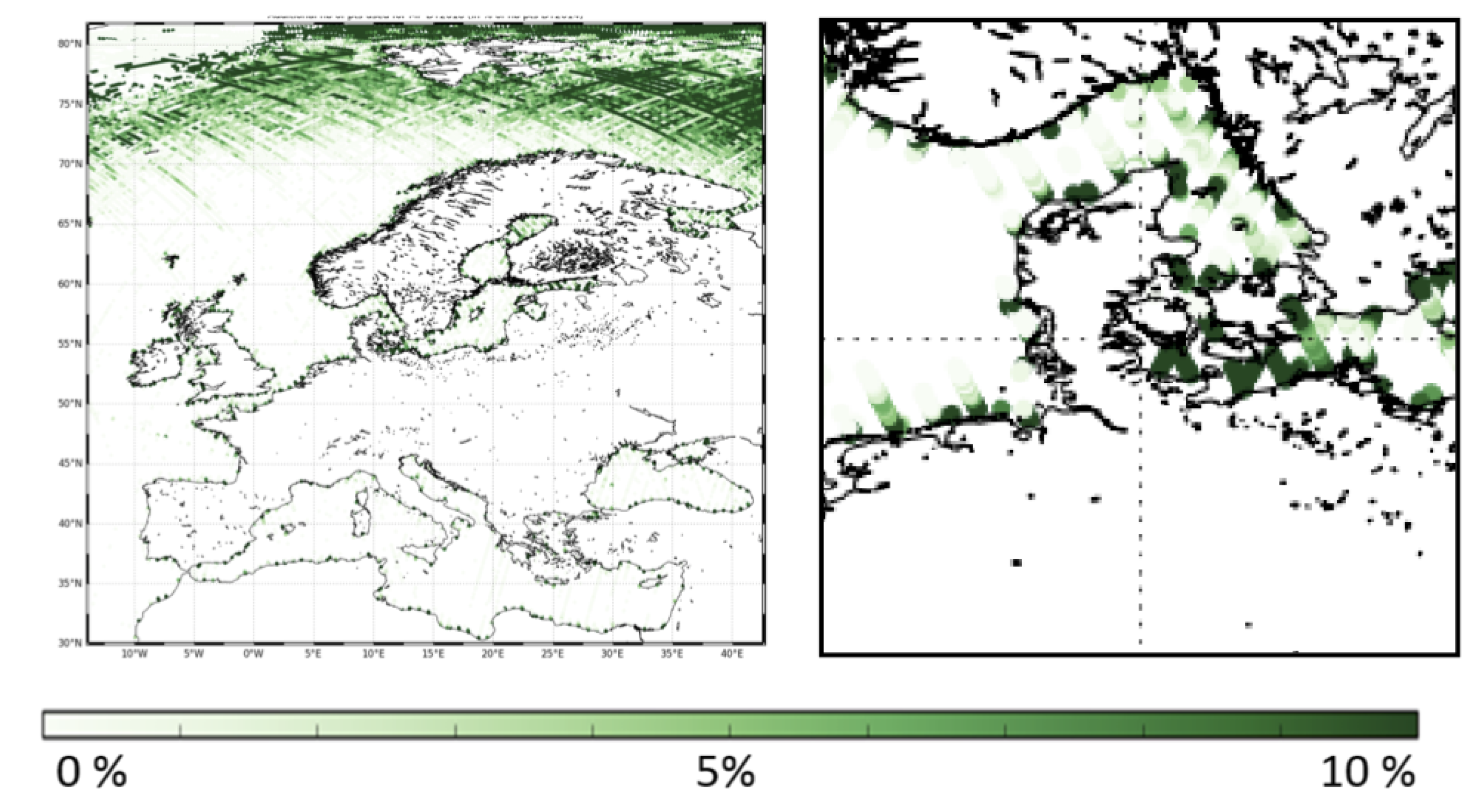
2.3.3. Assimilation of SWH Data Into the Météo-France Operational Weather Forecast System
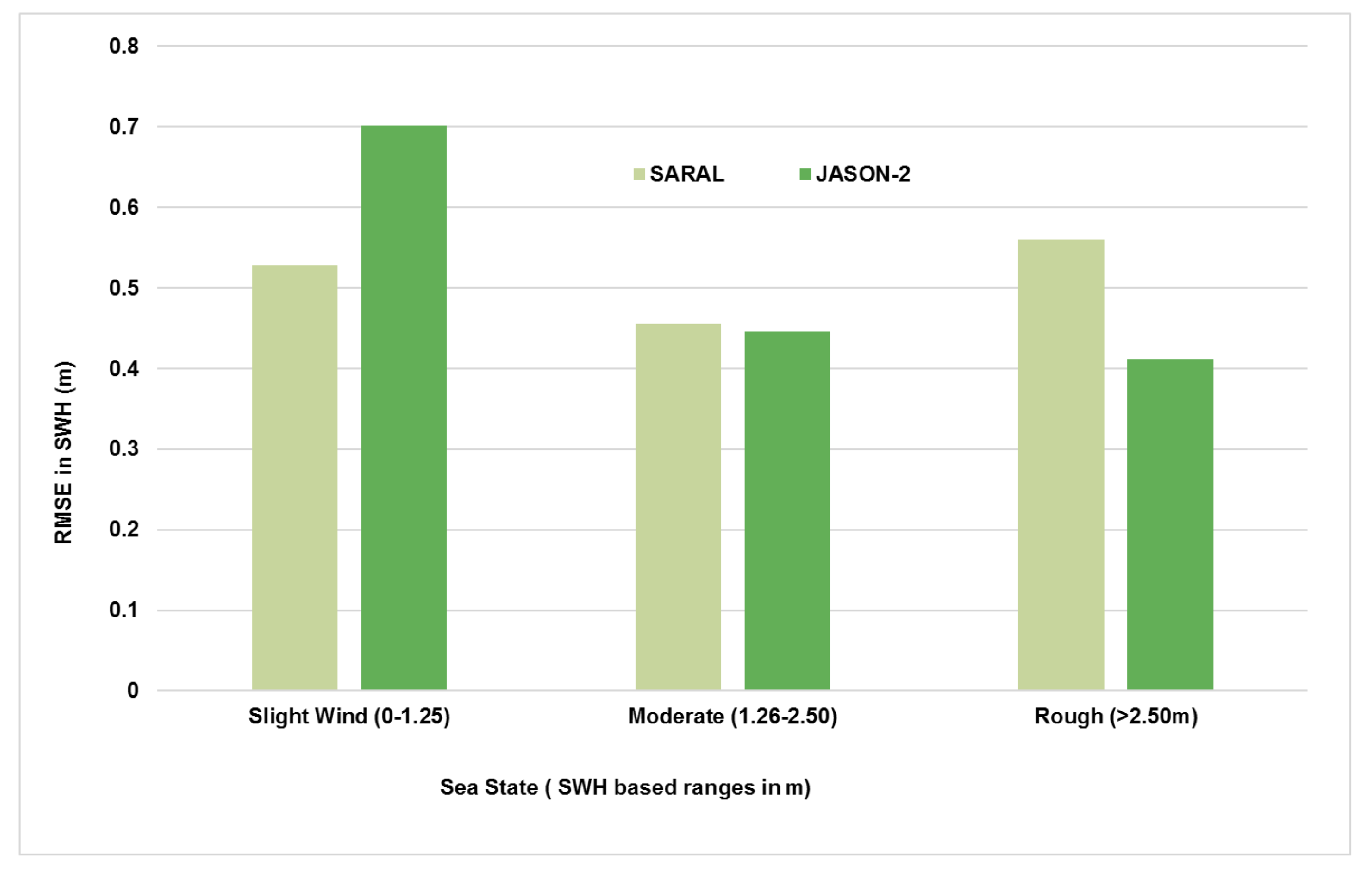
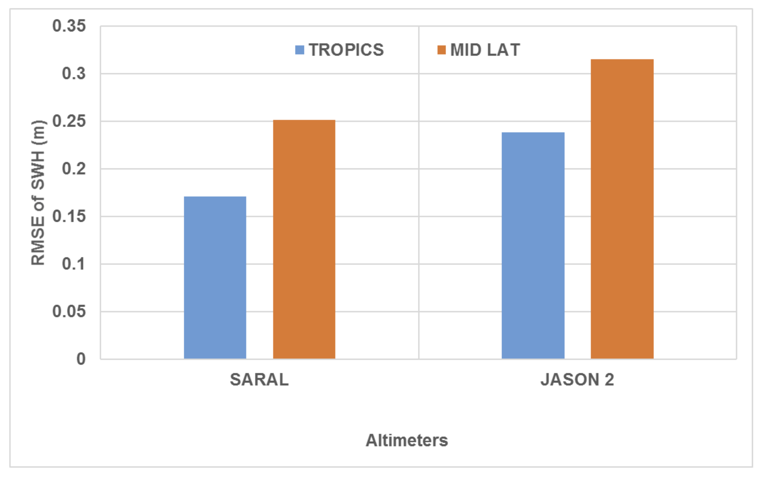
2.4. Accuracy of SWH Data
The Comparative Analysis of Ku and Ka-Band Altimeters for Wave Observations
3. Inland Waters
3.1. Rivers
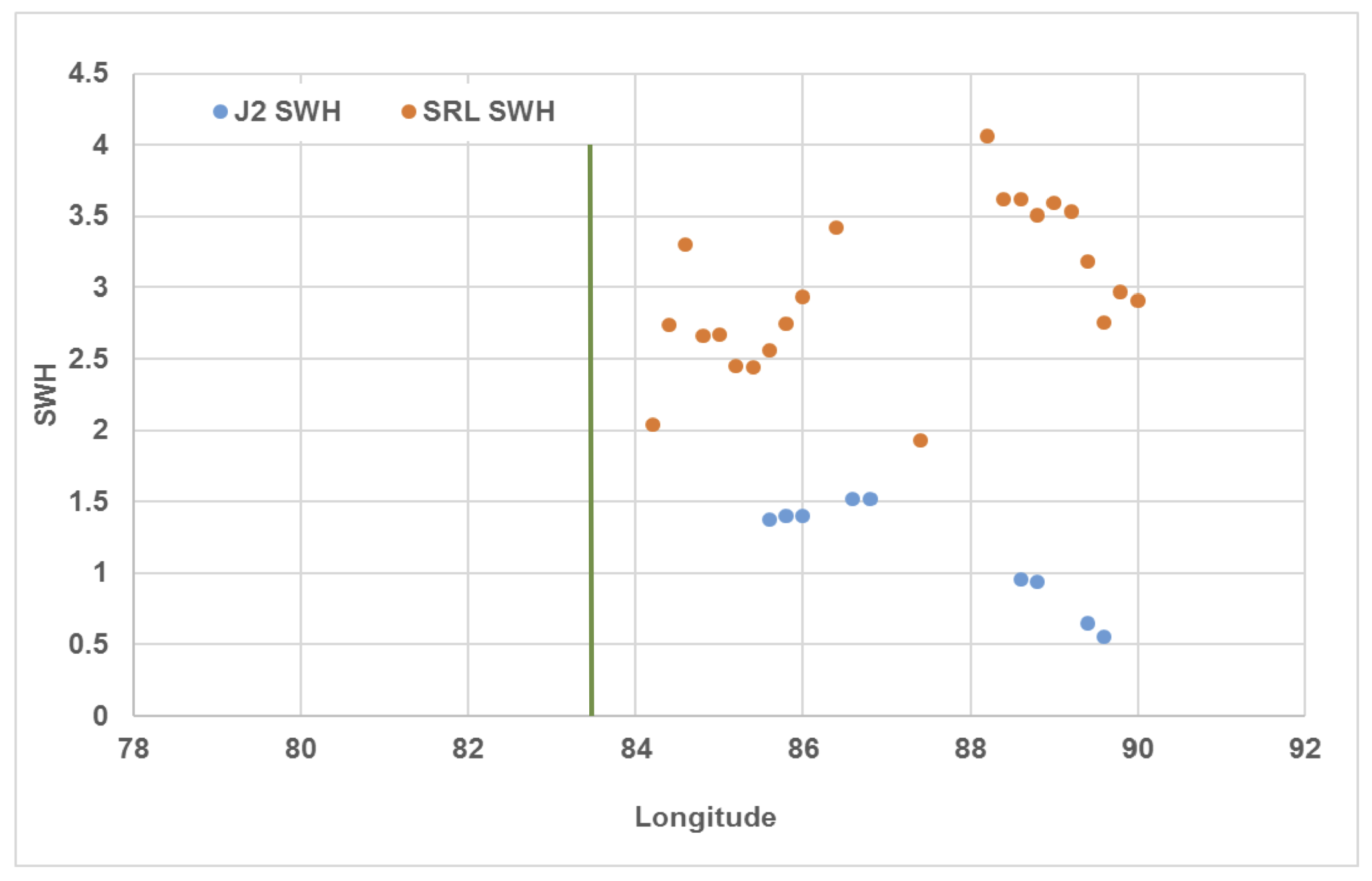
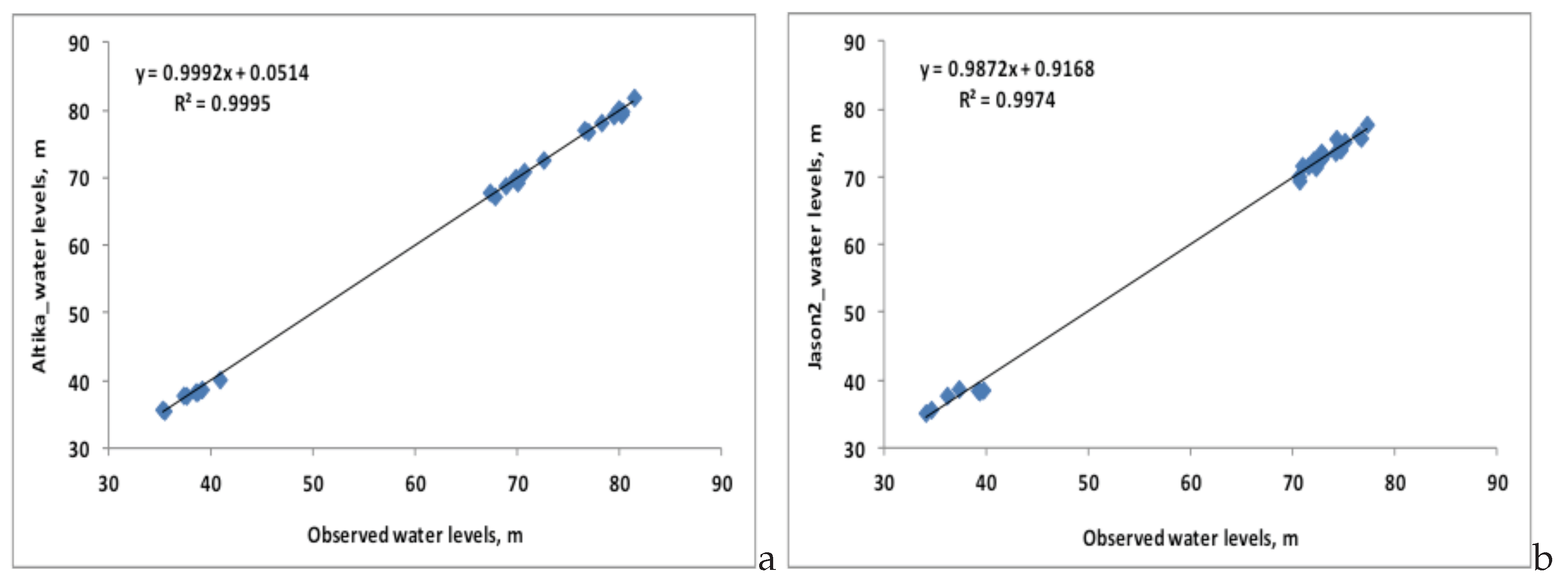
3.1.1. Comparative Analysis of Water Level Retrieval Using Ku and Ka-Band Altimeters Over Brahmaputra River
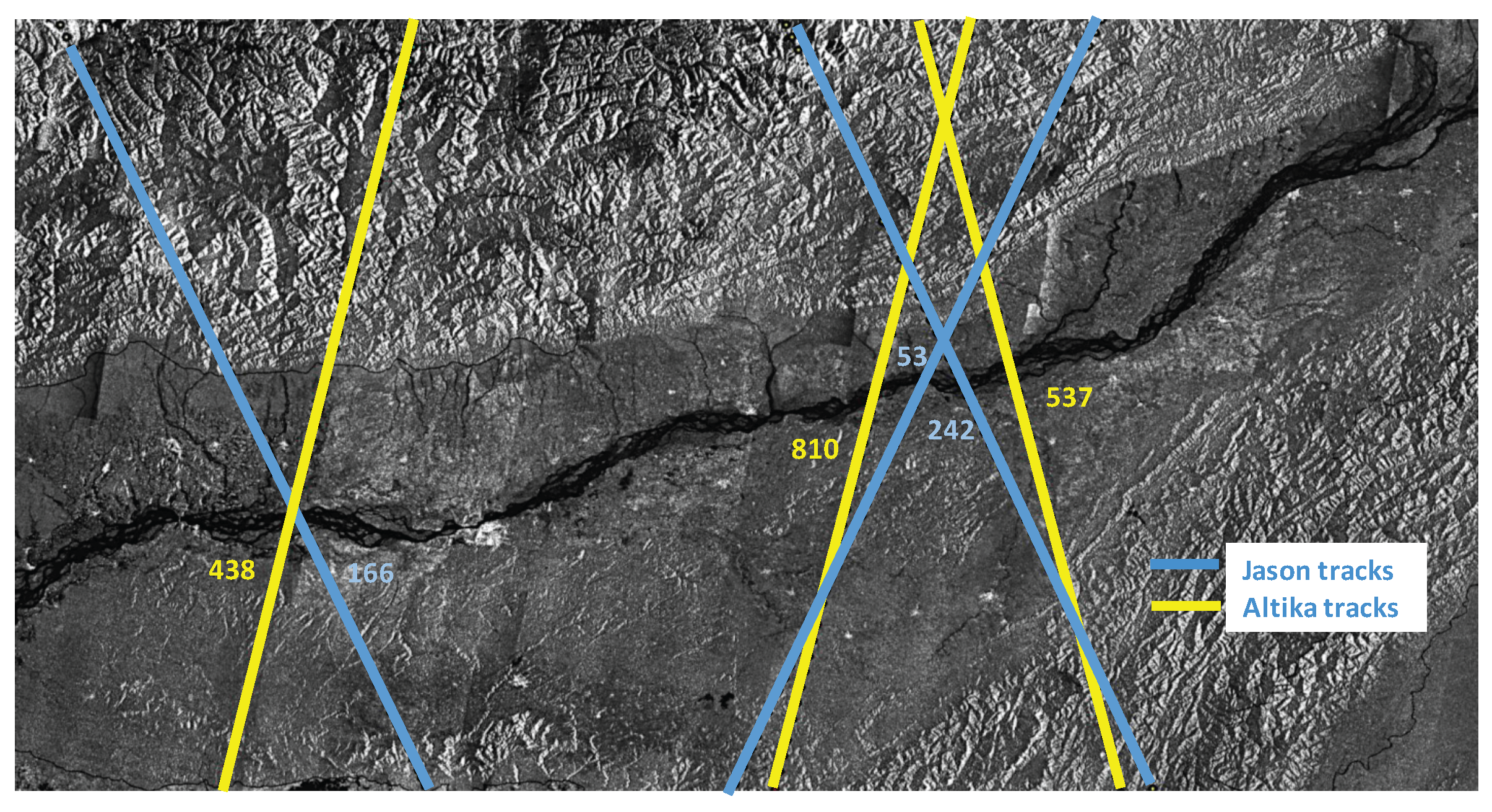
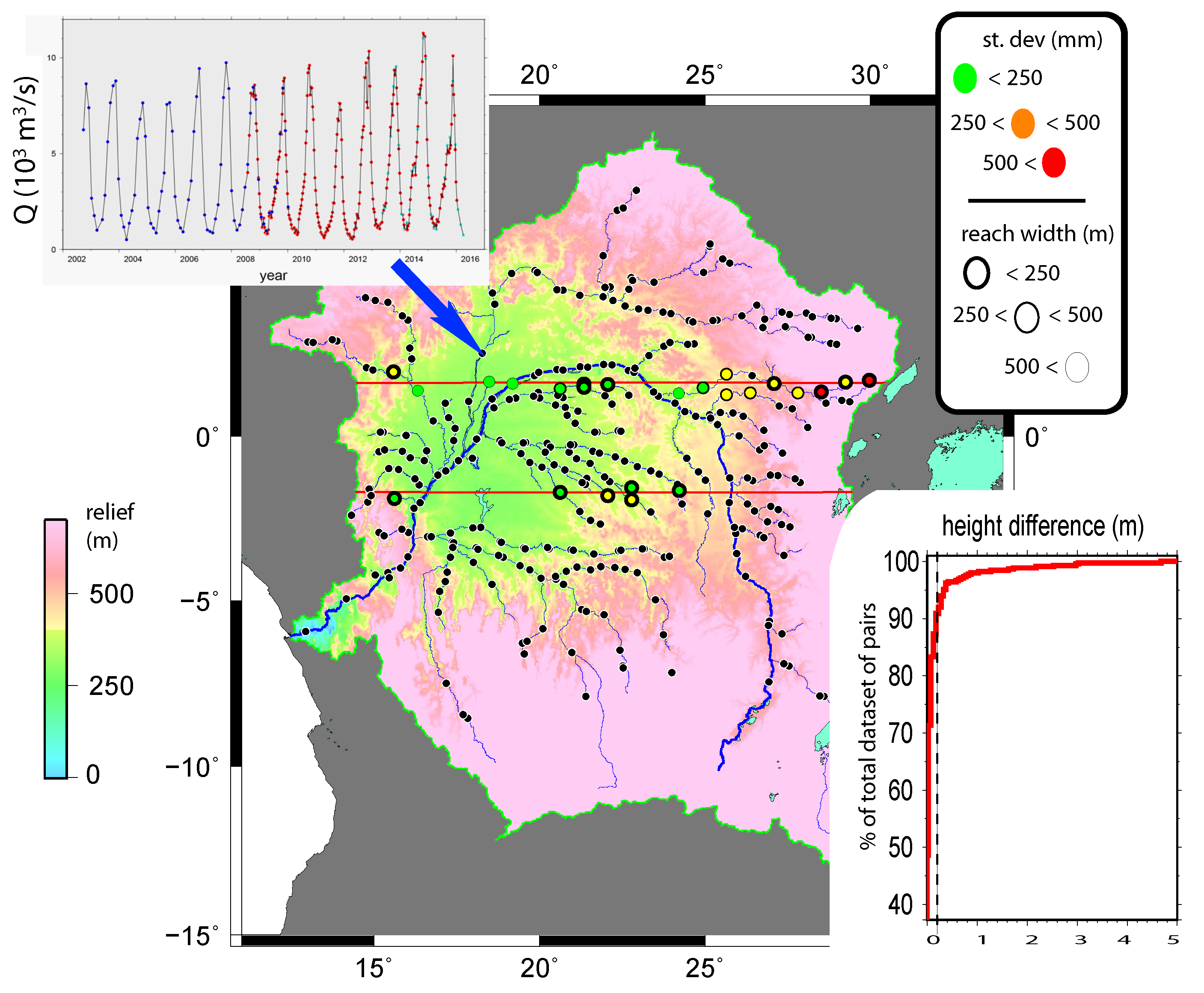
3.1.2. Discharge Estimates in the Congo Basin From Validated SARAL/AltiKa Measurements
3.2. Lakes
A Case Study of the Tibetan Lakes
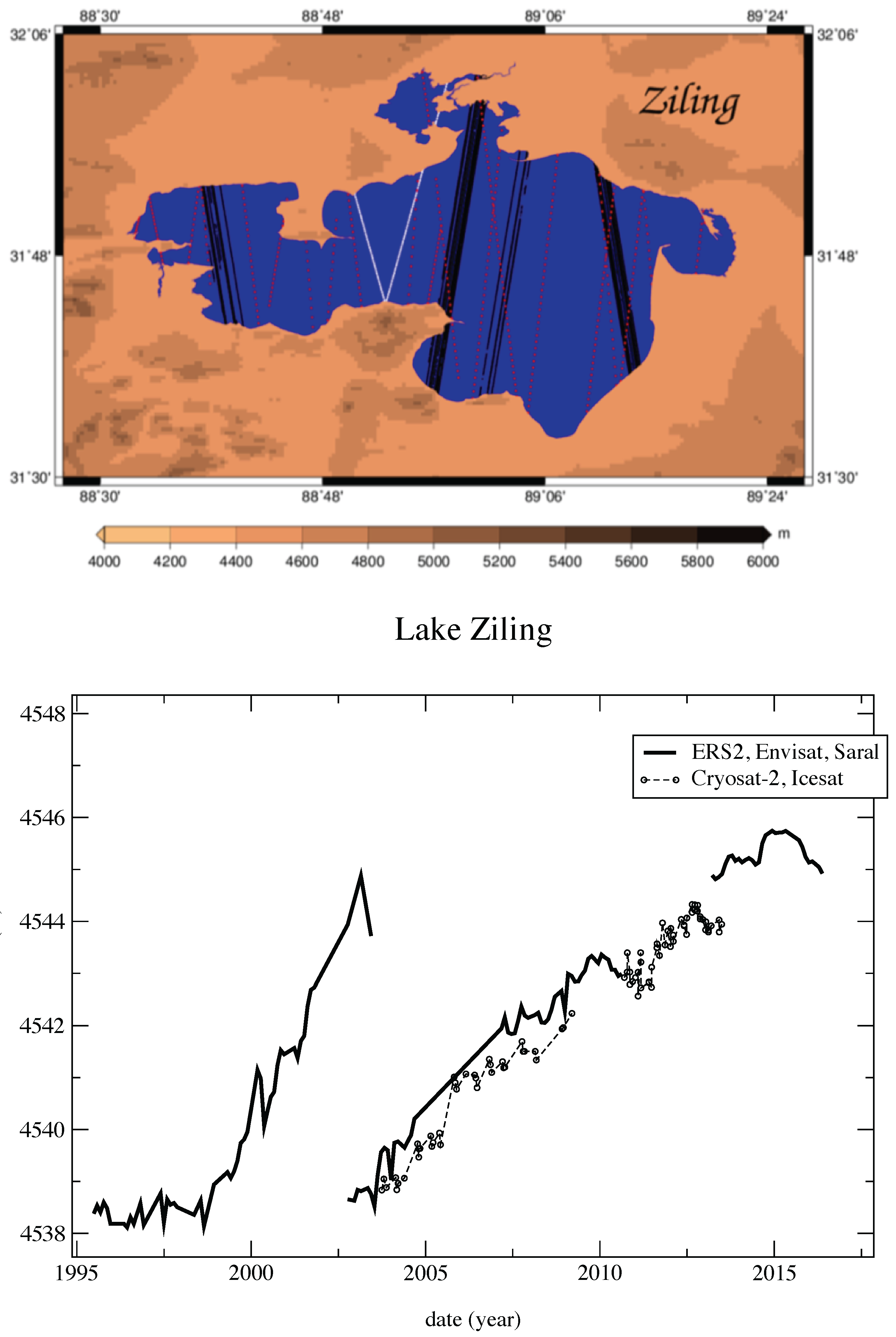
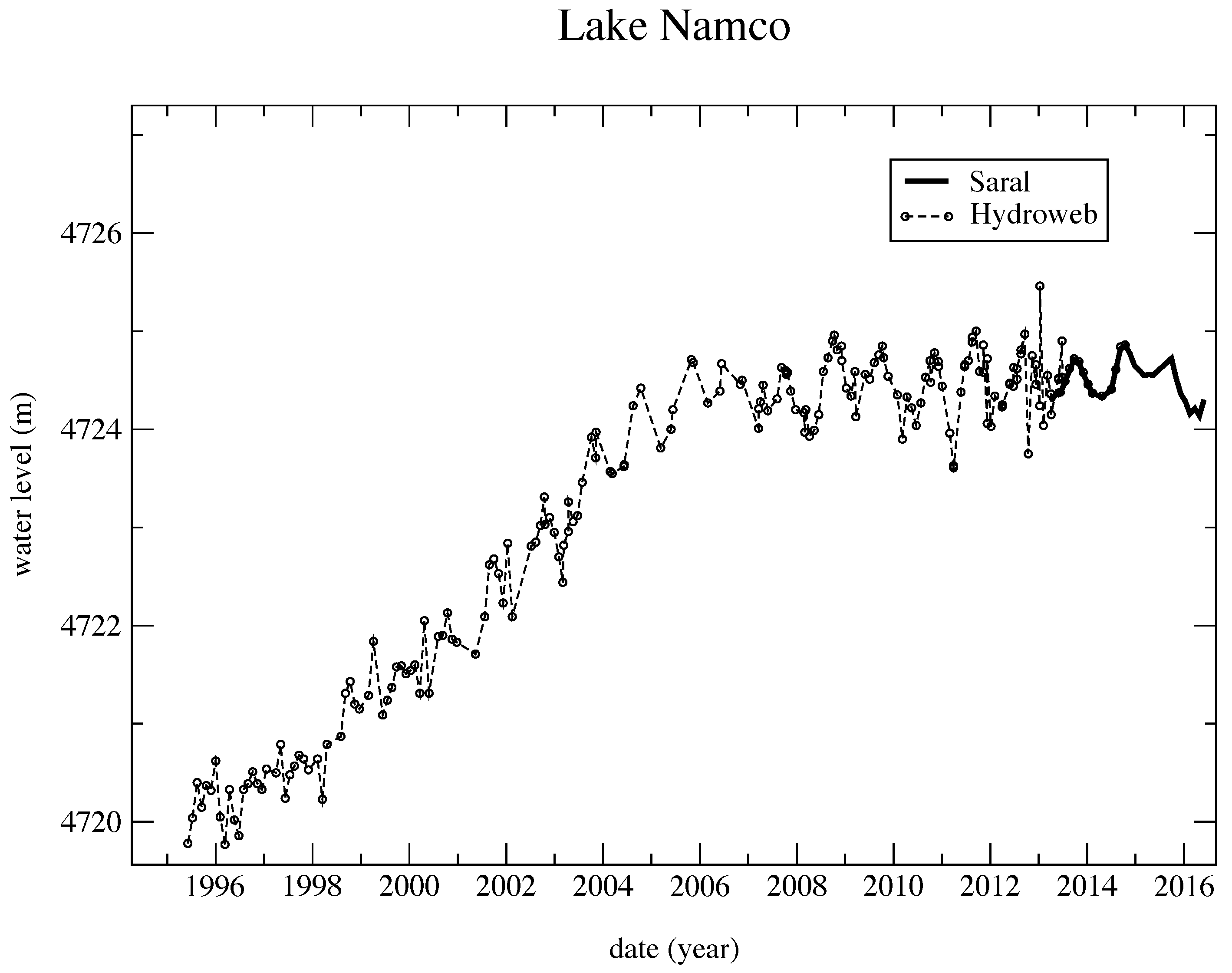
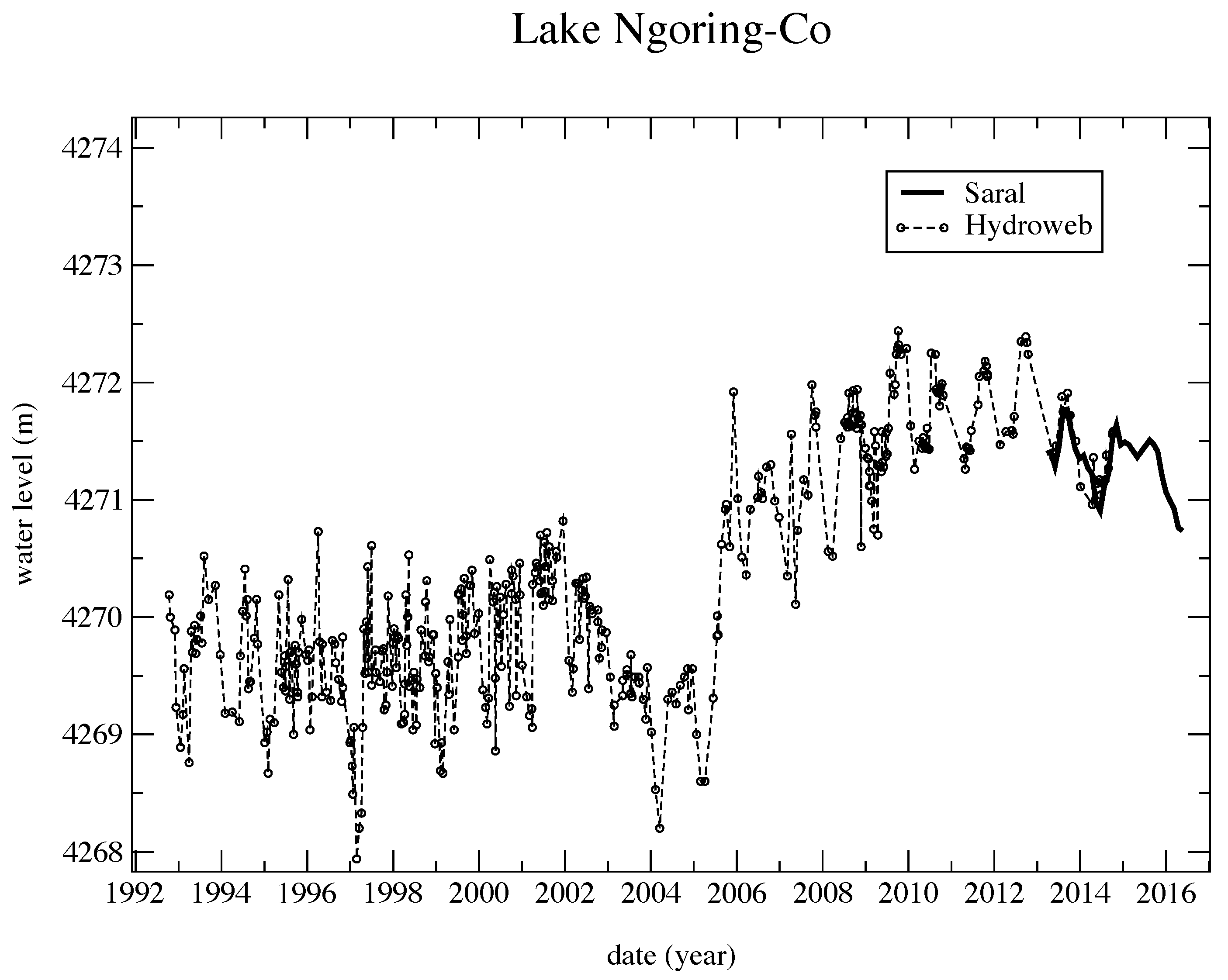
- The responses of lakes to climate changes are not the same from one lake to another one and needs long term observations to be highlighted. For example, the Ziling lake which has grew up during more than 15 years seems over the last years to reach an equilibrium state which has been seen only with the SARAL/AltiKa measurements. It may be different for other lakes, as seen in Figure 20 and Figure 21. It has been shown in [20] that long term changes of lakes over the Tibetan Plateau are highly variable and depend on regional climate change as well as the lake’s bathymetry.
- Only SARAL/AltiKa allows extracting short term variability of water level of these lakes, since the other missions (ERS-2, Envisat, CryoSat-2, TOPEX/Poseidon, Jason-1 and Jason-2) were not precise enough to show these seasonal variabilities.
4. Ice
4.1. Ice Sheet
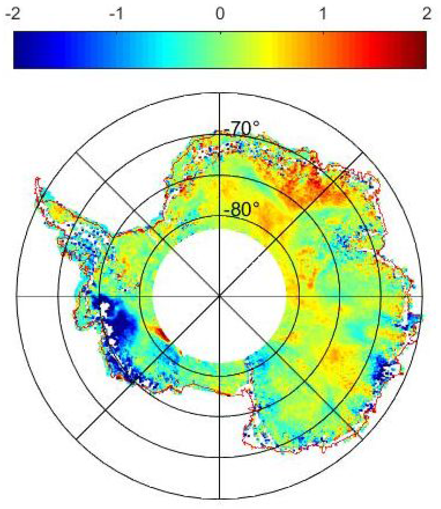
Monitoring of the Antarctic Ice Sheet
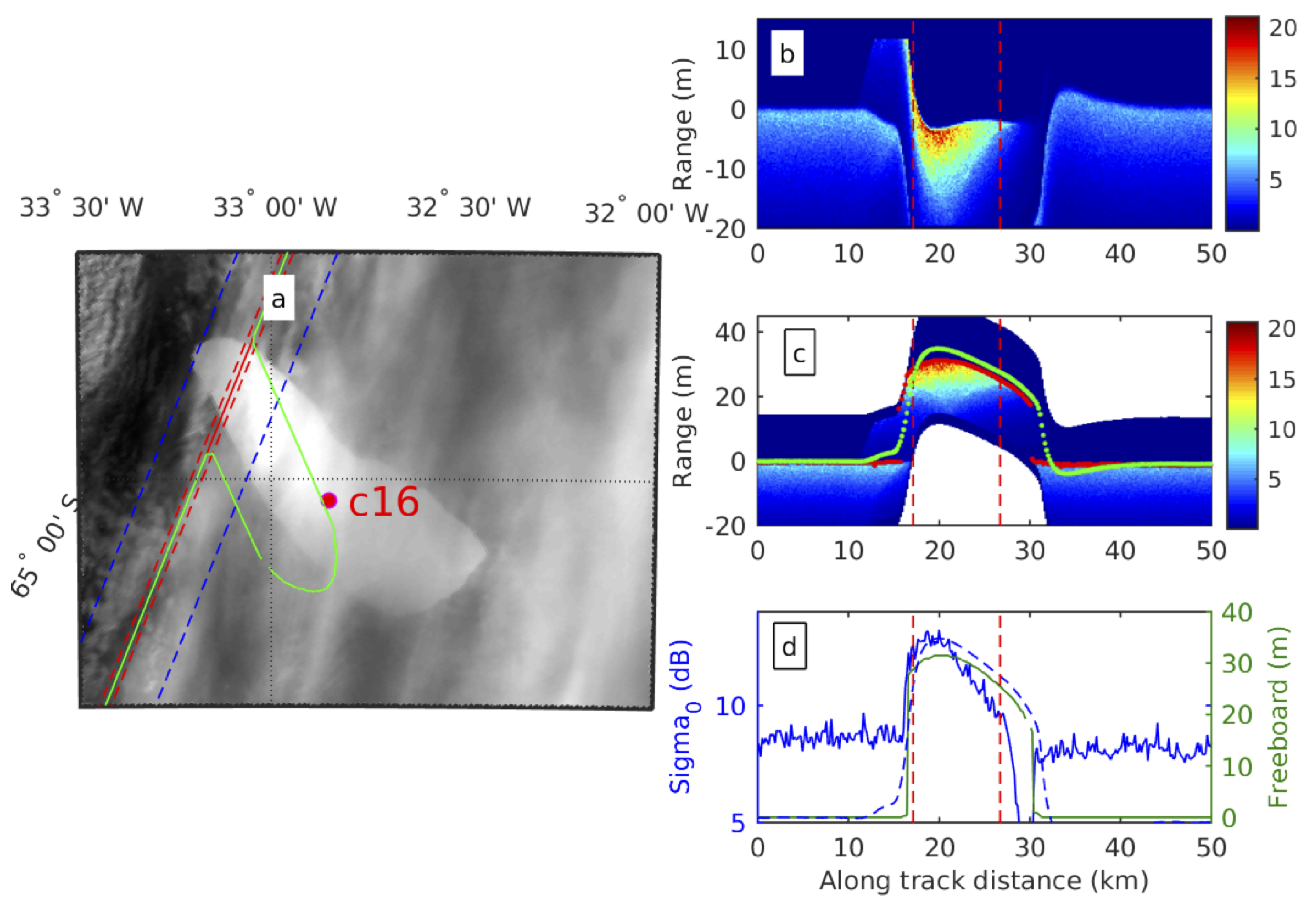
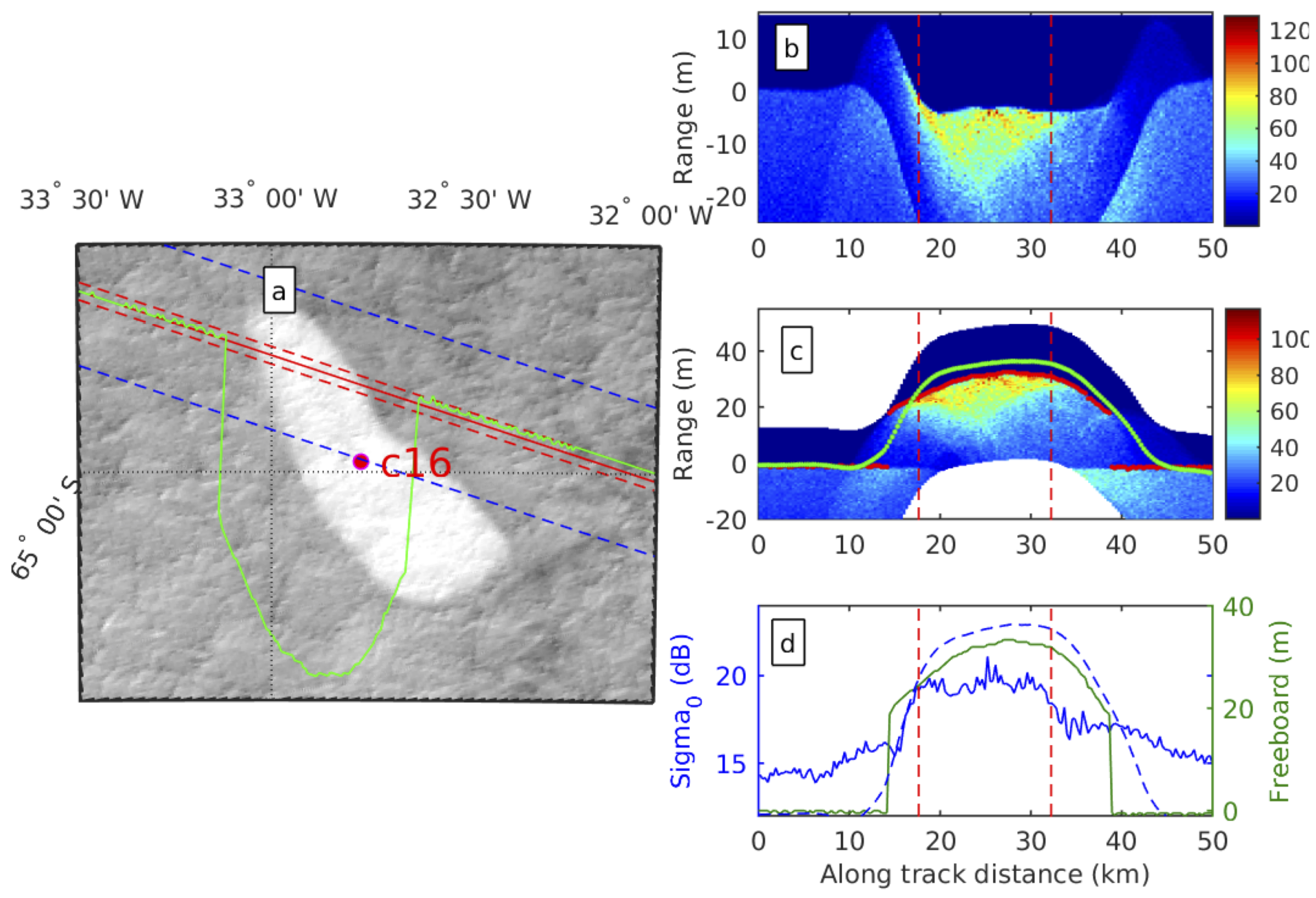
4.2. Icebergs
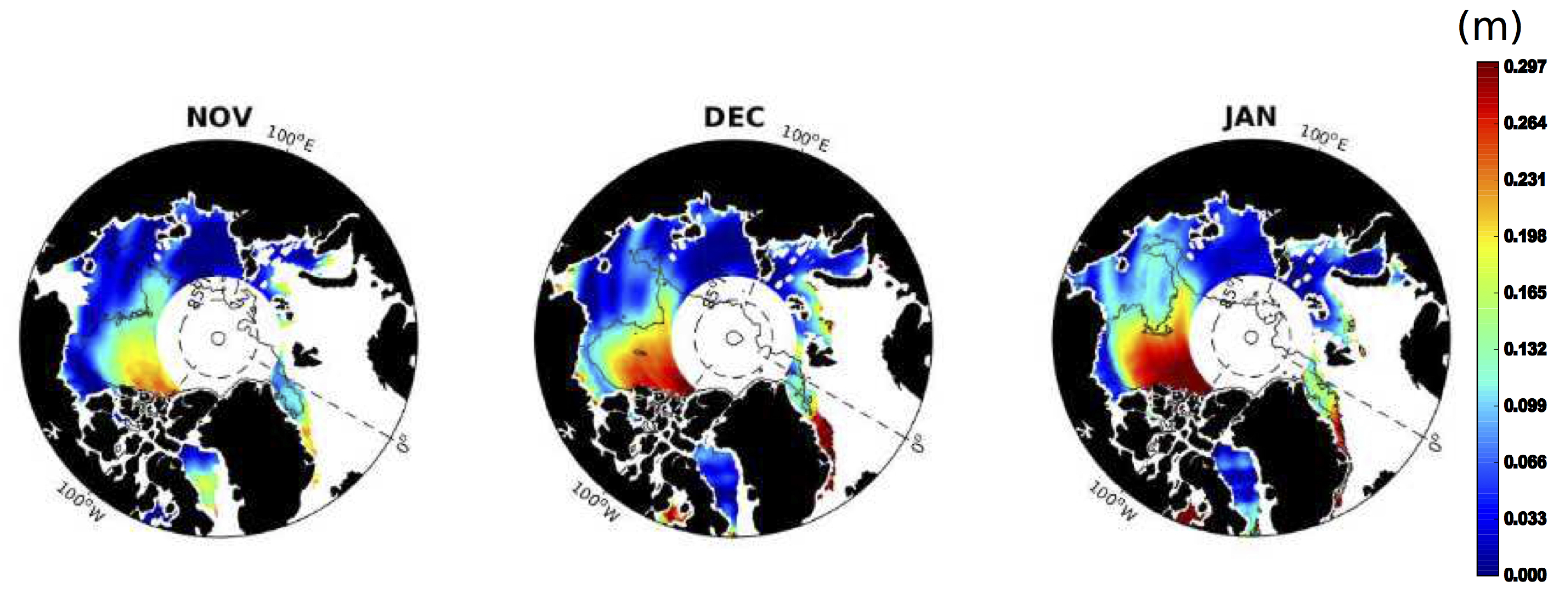
4.3. Sea Ice
- First, its smaller footprint, higher vertical resolution (∼30 cm) and higher horizontal sampling (∼180 m) allow a better discrimination between ice floes and open sea ice fractures (generally referred to as leads), which strongly improves the measurement of sea level and freeboard height. These improvements are somehow counter-balanced by the technical issue of waveform saturation while the altimeter overflight surfaces with highly variable scattering. This effect tends to degrade the range estimation during the approach phase of specular surfaces like leads. However, the reactivity of the Attenuation Gain Controller can be easily corrected in future altimeter version.
- The second advantage of SARAL/AltiKa lies on its higher radar frequency: Unlike Ku-band radar altimeters, the Ka-band radar signal of AltiKa penetrates only part of the snowpack and possibly less than 3 cm [43]. The latter study uses this difference of penetration depth between Ku- and Ka-band altimeters to estimate a proxy of snow depth at the top of sea ice by combining SARAL/AltiKa (Ka-band) and CryoSat-2/SIRAL (Ku-band) (Figure 25). As the uncertainty related to the impact of snow depth on the freeboard-to-thickness conversion can be up to 100 %, this opportunity of measuring snow depth from Ka- and Ku-band radar altimetry represents a real breakthrough. In addition to the freeboard-to-thickness conversion, the snow depth measurement could be of hight interest for the quantification of energy, transfer between the atmosphere and the ocean as well as for the estimation of freshwater fluxes in the ocean.
5. Geodesy
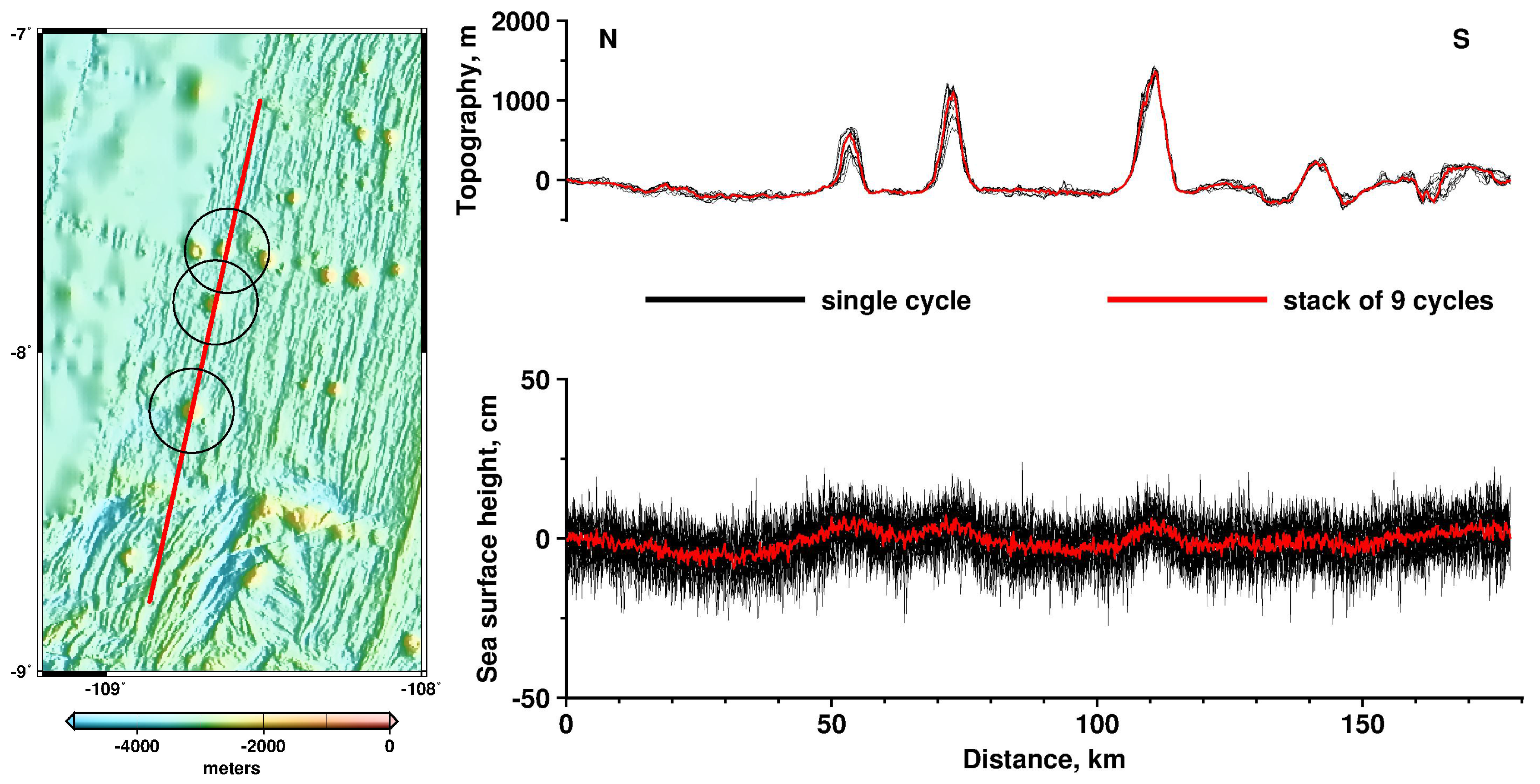
Ability to Find Uncharted Seamounts
6. Conclusions
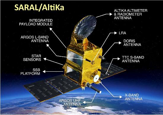
- The higher frequency (35.75 GHz, to be compared to 13.5 GHz on Jason-2) leads to a smaller footprint (8 km diameter, to be compared to 20 km on Jason-2 and to 15 km for Envisat) and thus a better horizontal resolution.
- Ka-band allows to use a larger bandwidth (480 MHz to be compared to 320 MHz on Jason-2). This 480 MHz bandwidth provides a high vertical resolution (0.3 m) which is better with respect to other altimeters.
- The higher Pulse Repetition Frequency (4 kHz to be compared to 2 kHz on Jason-2) permits a decorrelation time of sea echoes at Ka-band shorter than at Ku-band, then allowing a better along-track sampling. This makes possible to increase significantly the number of independent echoes per second compared with Ku-band altimeters.
- Ka-band is much less affected by the ionosphere than one operating at Ku-band. This low ionospheric attenuation can even be considered as negligible, except for some exceptional ionospheric situations. It discards the need for a dual-frequency altimeter.
- Ka-band provides a better estimation of sea surface roughness than at Ku-band. The 8 mm wavelength in Ka-band is better suited to describing the slopes of small facets on the sea surface (capillary waves, etc.) and gives a more accurate measurement of the backscatter coefficient over calm or moderate seas, thus leading to a noise reduction of a factor of two compared to Jason-class altimeters for wave heights greater than 1 m. Moreover, the specificities of the Ka-band backscatter coefficient offer unique contributions in fields that where not foreseen (snow/ice morphology and its temporal variability (Section 4), soil moisture [4], etc.).
- With Ka-band, there is a lower radar penetration of snow and ice: penetration of snowpack is less than 3 cm for snow on sea ice and 1 m for continental ice, around ten times less than for Ku-band. The altimetric observation and height restitution thus correspond to a thin subsurface layer.
- A possible drawback of Ka-band was that the attenuation due to water or water vapour in the troposphere might affect Ka-band pulses in case of rain and increase significantlly the rate of missing data for strong rain rates. In fact, this was not found to be true in practice and rain had little influence on data availability and quality.
Acknowledgments
Author Contributions
Conflicts of Interest
References
- Vincent, P.; Steunou, N.; Caubet, E.; Phalippou, L.; Rey, L.; Thouvenot, E.; Verron, J. AltiKa: A Ka-band altimetry payload and system for operational altimetry during the GMES period. Sensors 2006, 6, 208–234. [Google Scholar] [CrossRef]
- Verron, J.; Sengenes, P.; Lambin, J.; Noubel, J.; Steunou, N.; Guillot, A.; Picot, N.; Coutin-Faye, S.; Gairola, R.; Raghava Murthy, D.V.A.; et al. The SARAL/AltiKa altimetry satellite mission. Mar. Geodesy 2015, 38, 2–21. [Google Scholar] [CrossRef]
- The SARAL/AltiKa Satellite Altimetry Mission. Mar. Geodesy 2015, 38. Available online: http://www.tandfonline.com/toc/umgd20/38/sup1 (accessed on 12 January 2018).
- Bonnefond, P.; Verron, J.; Aublanc, J.; Babu, K.N.; Bergé-Nguyen, M.; Cancet, M.; Chaudhary, A.; Crétaux, J.F.; Frappart, F.; Haines, B.J.; et al. The benefits of the Ka-band as evidenced from the SARAL/AltiKa altimetric mission: Quality assessment and specificities of AltiKa data. Remote Sens. 2018, 10, 83. [Google Scholar] [CrossRef]
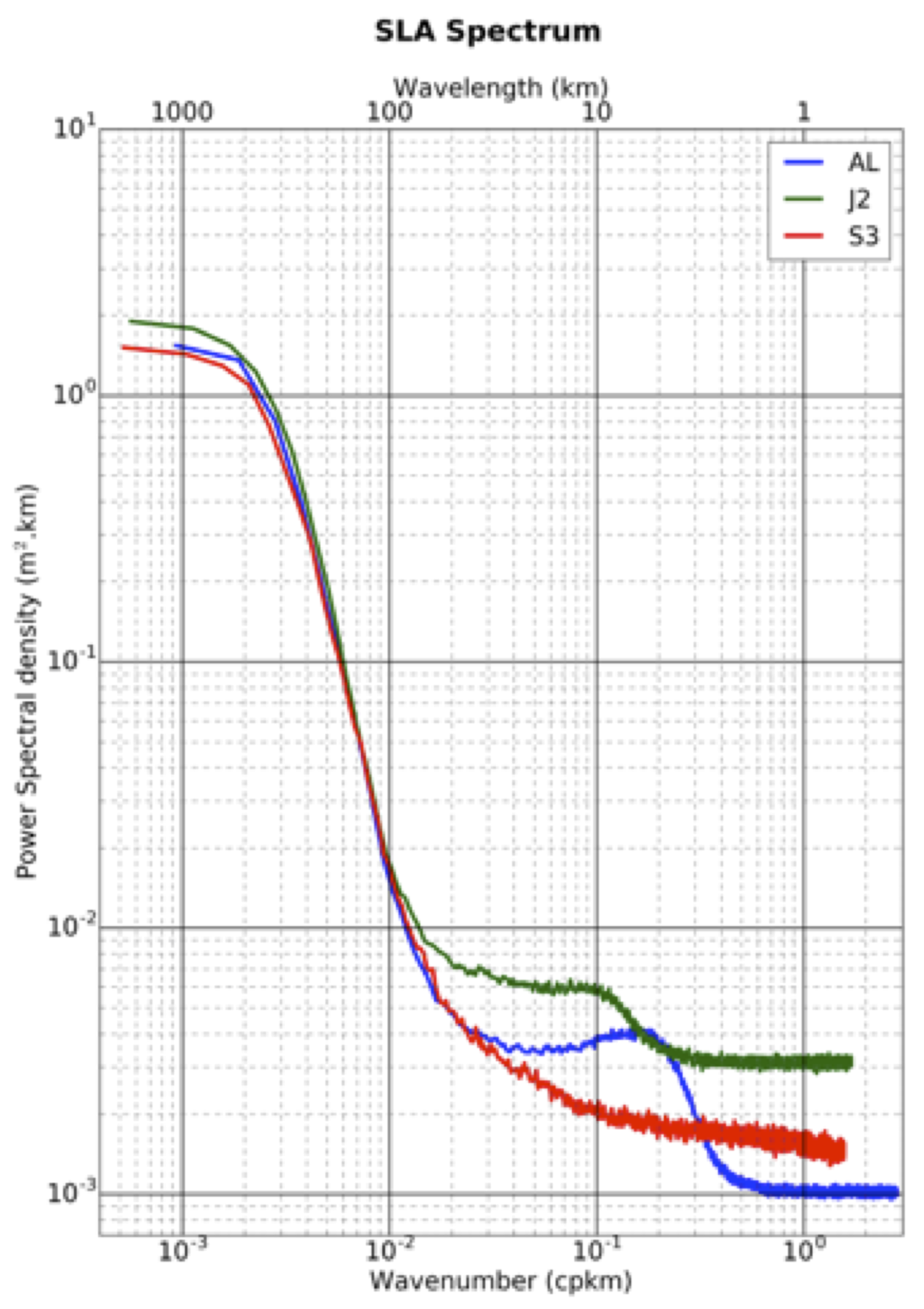
- Dufau, C.; Orsztynowicz, M.; Dibarboure, G.; Morrow, R.; Le Traon, P.Y. Mesoscale Resolution Capability of altimetry: Present & future. J. Geophys. Res. Oceans 2016, 121, 4910–4927. [Google Scholar]
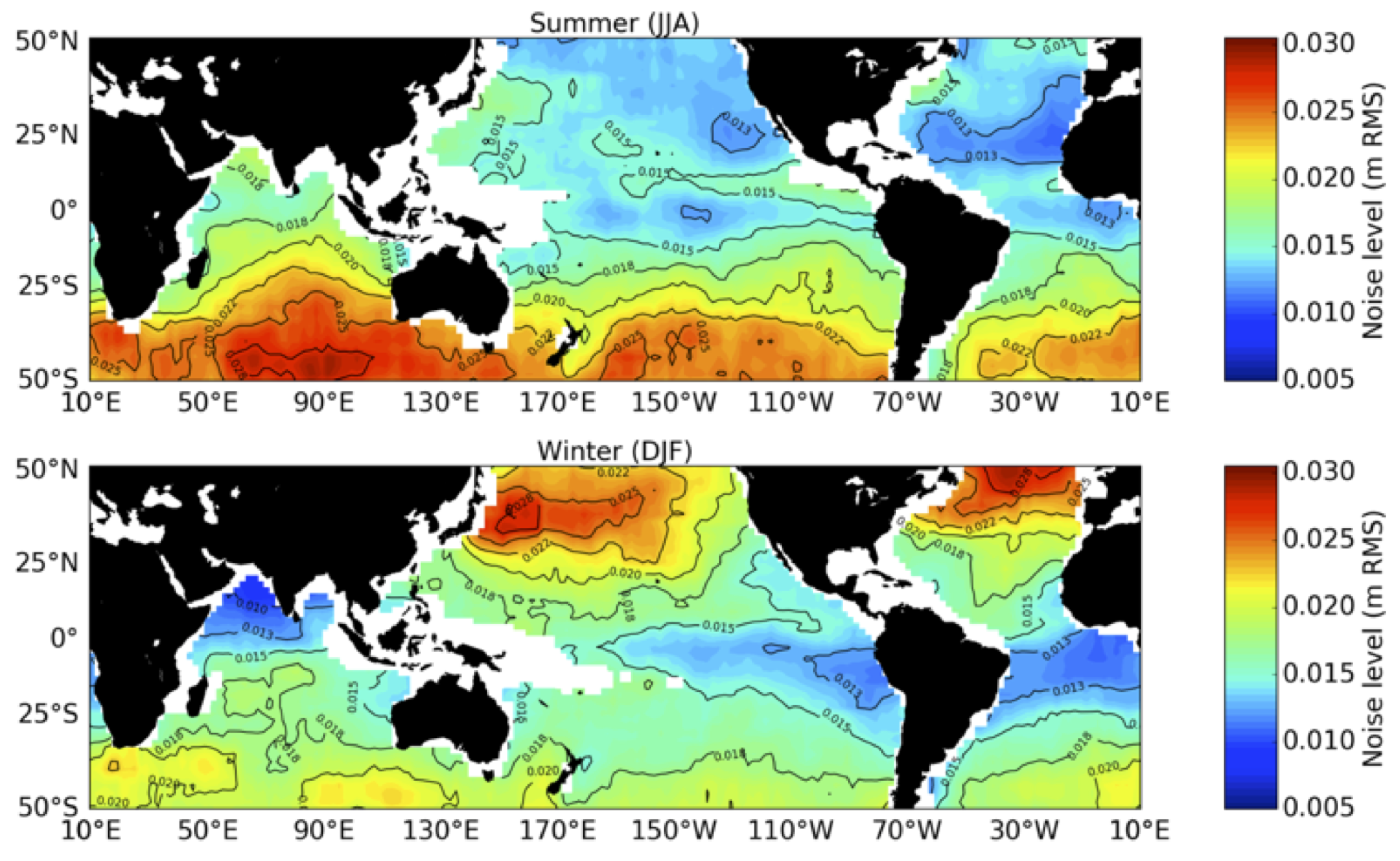
- Ablain, M.; Raynal, M.; Lievin, M.; Thibaut, P.; Dibarboure, G.; Picot, N. Improving altimeter sea level calculation at small ocean scales. In Proceedings of the 2016 Ocean Surface Topography Science Team (OSTST) Meeting, La Rochelle, France, 31 October–1 November 2016. [Google Scholar]
- Morrow, R.; Carret, A.; Birol, F.; Nino, F.; Valladeau, G.; Boy, F.; Bachelier, C.; Zakardjian, B. Observability of fine-scale ocean dynamics in the Northwest Mediterranean Sea. Ocean Sci. 2017, 13, 13–29. [Google Scholar] [CrossRef]
- Dibarboure, G.; Pujol, M.I.; Briol, F.; Le Traon, P.Y.; Larnicol, G.; Picot, N.; Mertz, F.; Ablain, M. Jason-2 in DUACS: Updated System Description, First Tandem Results and Impact on Processing and Products. Mar. Geodesy 2011, 34, 214–241. [Google Scholar] [CrossRef]
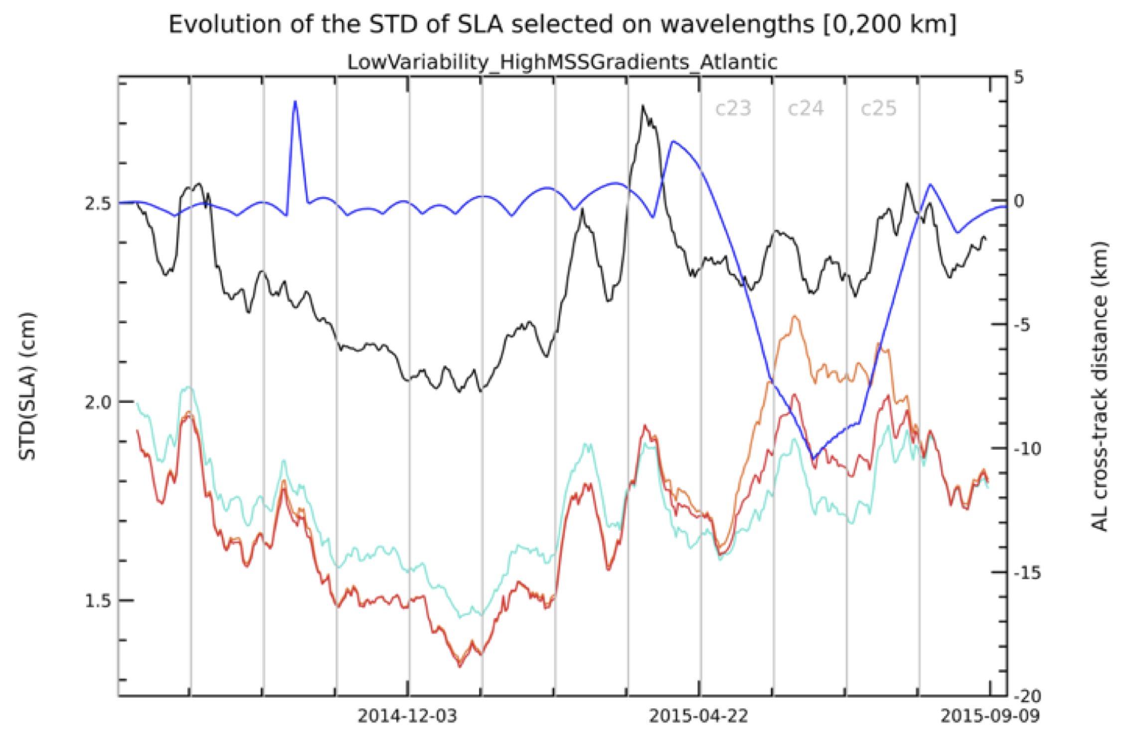
- Pujol, M.-I.; Schaeffer, P.; Faugére, Y.; Raynal, M.; Dibarboure, G.; Picot, N. Gauging the improvement of recent mean sea surface models: A new approach for identifying and quantifying their errors. J. Geophys. Res. 2017, submitted. [Google Scholar]
- Jebri, F.; Birol, F.; Zakardjian, B.; Bouffard, J.; Sammari, C. Exploiting coastal altimetry to improve the surface circulation scheme over the central Mediterranean Sea. J. Geophys. Res. Ocean. 2016, 121, 4888–4909. [Google Scholar] [CrossRef]
- Sorgente, R.; Olita, A.; Oddo, P.; Fazioli, L.; Ribotti, A. Numerical simulation and decomposition of kinetic en e.g., in the Central Mediterranean: Insight on mesoscale circulation and en e.g., conversion. Ocean Sci. 2011, 7, 503–519. [Google Scholar] [CrossRef] [Green Version]
- Rubio, A.; Mader, J.; Corgnati, L.; Mantovani, C.; Griffa, A.; Novellino, A.; Quentin, C.; Wyatt, L.; Schulz-Stellenfleth, J.; Horstmann, J.; et al. HF Radar Activity in European Coastal Seas: Next Steps toward a Pan-European HF Radar Network. Front. Mar. Sci. 2017, 4, 8. [Google Scholar] [CrossRef]
- Pascual, A.; Lana, A.; Troupin, C.; Ruiz, S.; Faugère, Y.; Escudier, R. Assessing SARAL/AltiKa delayed-time data in the coastal zone: Comparisons with HFR observations. Mar. Geodesy 2015, 38, 260–276. [Google Scholar] [CrossRef]
- Rio, M.-H.; Pascual, A.; Poulain, P.-M.; Menna, M.; Barcelò-Llull, B.; Tintoré, J. Computation of a new mean dynamic topography for the Mediterranean Sea from model outputs, altimeter measurements and oceanographic in-situ data. Ocean Sci. 2014, 10, 731–744. [Google Scholar] [CrossRef]
- Pujol, M.I.; Faugère, Y.; Taburet, G.; Dupuy, S.; Pelloquin, C.; Ablain, M.; Picot, N. DUACS DT2014: The new multi-mission altimeter dataset reprocessed over 20 years. Ocean Sci. 2016, 12, 1067–1090. [Google Scholar] [CrossRef]
- Le Traon, P.Y.; Antoine, D.; Bentamy, A.; Bonekamp, H.; Breivik, L.A.; Chapron, B.; Corlett, G.; Dibarboure, G.; Digiacomo, P.; Donlon, C.; et al. Use of satellite observations for operational oceanography: Recent achievements and future prospects. J. Oper. Ocean. 2015, 8 (Suppl. 1), 12–27. [Google Scholar] [CrossRef]
- Desroziers, G.; Berre, L.; Chapnik, B.; Poli, P. Diagnosis of observation, background and analysis-error statistics in observation space. Quart. J. R. Meteorol. Soc. 2005, 131, 3385–3396. [Google Scholar] [CrossRef]
- Calmant, S.; Seyler, F. Continental surface waters from satellite altimetry. Géosciences 2006, 338, 1113–1122. [Google Scholar] [CrossRef]
- Crétaux, J.F.; Birkett, C. Lake studies from satellite radar altimetry. Comptes Rendus Geosci. 2006, 338, 1098–1112. [Google Scholar]
- Crétaux, J.-F.; Abarca Del Rio, R.; Berge-Nguyen, M.; Arsen, A.; Drolon, V.; Clos, G.; Maisongrande, P. Lake volume monitoring from Space. Surv. Geophys. 2016, 37, 269–305. [Google Scholar] [CrossRef]
- Alsdorf, D.; Beighley, E.; Laraque, A.; Lee, H.; Tshimanga, R.; O’Loughlin, F.; Dinga, B.; Moukandi, G.; Spencer, R.G. Opportunities for hydrologica research in the Congo basin. Rev. Geophys. 2016, 54, 378–409. [Google Scholar] [CrossRef]
- Laraque, A.; Bellanger, M.; Adèle, G.; Guebanda, S.; Gulemvuga, G.; Pandi, A.; Paturel, J.E.; Robert, A.; Tathy, J.P.; Yambele, A. Recent evolution of Congo, Oubangui and Sangha Rivers flows. Acad. R. Sci. Belgique Geogr. Ecol. Trop. 2013, 37, 93–100. [Google Scholar]
- Silva, J.; Calmant, S.; Seyler, F.; Medeiros Moreira, D.; Oliveira, D.; Monteiro, A. Radar Altimetry aids Managing gauge networks. Water Resour. Manag. 2014, 28, 587–603. [Google Scholar] [CrossRef]
- Dubey, A.K.; Gupta, P.; Dutta, S.; Pratap Sing, R. Water Level retrieval Using SARAL/AltiKa Observations in the braided Brahmapoutra River, Eastern India. Mar. Geodesy 2015, 38, 549–567. [Google Scholar] [CrossRef]
- Frappart, F.; Papa, F.; Marieu, V.; Malbeteau, Y.; Jordy, F.; Calmant, S.; Durand, F.; Bala, S. Preliminary assessment of SARAL/AltiKa observations over the Ganges-Brahmaputra and Irrawaddy Rivers. Mar. Geodesy 2015, 38, 568–580. [Google Scholar] [CrossRef]
- Schwatke, C.; Dettmering, D.; Borgens, E.; Bosch, W. Potential of SARAL/Altika for Inland Water Application. Mar. Geodesy 2015, 38, 626–643. [Google Scholar] [CrossRef]
- Frappart, F.; Calmant, S.; Cauhopé, M.; Seyler, F.; Cazenave, A. Results of Envisat RA-2 Derived levels Validation over the Amazon basin. Remote Sens. Environ. 2006, 100, 252–264. [Google Scholar] [CrossRef] [Green Version]
- Silva, J.; Calmant, S.; Rotuono Filho, O.; Seyler, F.; Cochonneau, G.; Roux, E.; Mansour, J.W. Water Levels in the Amazon basin derived from the ERS-2 and Envisat Radar Altimetry Missions. Remote Sens. Environ. 2010, 114, 2160–2181. [Google Scholar] [CrossRef]
- Paris, A.; Santos da Silva, J.; Dias de Paiva, R.; Medeiros Moreira, D.; Calmant, S.; Collischonn, W.; Bonnet, M.-P.; Seyler, F. Global determination of rating curves in the Amazon basin. Water Resour. Res. 2016, 28, 3787–3814. [Google Scholar] [CrossRef]
- Wang, B.; Bao, Q.; Hoskins, B.; Wu, G.; Liu, Y. Tibetan Plateau warming and precipitation change in East Asia. Geophys. Res. Lett. 2008, 35, L14702. [Google Scholar] [CrossRef]
- Liu, J.; Wang, S.; Yu, S.; Yang, D.; Zhang, L. Climate warming and growth of high-elevation inland lakes on the Tibetan Plateau. Glob. Planet. Chang. 2009, 67, 209–217. [Google Scholar] [CrossRef]
- Lei, Y.; Yang, K.; Wang, B.; Sheng, Y.; Bird, B.W.; Zhang, G.; Tian, L. Response of inland lake dynamics over the Tibetan Plateau to climate change. Clim. Chang. 2014, 125, 281–290. [Google Scholar] [CrossRef]
- Phan, V.H.; Lindenb, R.C.; Menenti, M. Geometric dependency of Tibetan lakes on glacial runoff. Hydrol. Earth Syst. Sci. Discuss. 2013, 10, 729–768. [Google Scholar] [CrossRef]
- Arsen, A.; Cretaux, J.-F.; Abarca-Del-Rio, R. Use of SARAL/AltiKa over mountainous lakes, intercomparison with Envisat mission. J. Adv. Space Res. 2015, 38, 534–548. [Google Scholar] [CrossRef]
- Remy, F.; Flament, T.; Michel, A.; Verron, J. Ice sheet survey over Antarctica with satellite altimetry: ERS-2, Envisat, SARAL/AltiKa, the key importance of continuous observations along the same repeat orbit. Int. J. Remote Sens. 2014, 35, 5497–5512. [Google Scholar] [CrossRef]
- Kouraev, A.; Zakharova, E.; Remy, F. Study of Lake Baikal ice cover from radar altimetry and in situ observations. Mar. Geodesy 2015, 38, 477–486. [Google Scholar] [CrossRef]
- Rémy, F.; Flament, T.; Michel, A.; Blumstein, D. Envisat and SARAL/AltiKa observations of the Antarctic ice sheet: A comparison between the Ku-band and the Ka-band. Mar. Geodesy 2015, 38, 510–521. [Google Scholar] [CrossRef]
- Tournadre, J. Signature of Lighthouses, Ships, and Small Islands in Altimeter Waveforms. J. Atmos. Ocean. Tech. 2007, 24, 1143–1149. [Google Scholar] [CrossRef]
- Tournadre, J.; Girard-Ardhuin, F.; Legresy, B. Antarctic iceb e.g., distributions, 2002–2010. J. Geophys. Res. 2012, 117, C05004. [Google Scholar] [CrossRef]
- Tournadre, J.; Bouhier, N.; Girard-Ardhuin, F.; Remy, F. Antarctic iceb e.g., distributions 1992–2014. J. Geophys. Res. 2016, 121, 327–349. [Google Scholar] [CrossRef]
- McIntyre, N.F.; Cudlip, W. Observation of a giant Antarctic tabular iceberg by satellite radar altimetry. Polar Rec. 1987, 145, 458–462. [Google Scholar] [CrossRef]
- Tournadre, J.; Bouhier, N.; Girard-Ardhuin, F.; Remy, F. Large iceb e.g., characteristics from altimeter waveforms analysis. J. Geophys. Res. 2015, 120, 1954–1974. [Google Scholar] [CrossRef]
- Guerreiro, K.; Fleury, S.; Zakharova, E.; Rémy, F.; Kouraev, A. Potential for estimation of snow depth on Arctic sea ice from CryoSat-2 and SARAL/AltiKa missions. Remote Sens. Environ. 2016, 186, 339–349. [Google Scholar] [CrossRef]
- Smith, W.H.F.; Barale, V.; Gower, J.; Alberotanza, L. The Marine Geoid and Satellite Altimetry. In Oceanography from Space; Springer: Dordrecht, The Netherlands, 2010. [Google Scholar]
- Wessel, P. Global distribution of seamounts inferred from gridded Geosat/ERS-1 altimetry. J. Geophys. Res. 2001, 109, 19431–19441. [Google Scholar] [CrossRef]
- Wessel, P.; Chandler, M.T. The spatial and temporal distribution of marine geophysical surveys. Acta Geophys. 2011, 59, 55–71. [Google Scholar] [CrossRef]
- Smith, W.H.F. The Resolution of Seamount Geoid Anomalies Achieved by the SARAL/AltiKa and Envisat RA2 Satellite Radar Altimeters. Mar. Geodesy 2015, 38, 644–671. [Google Scholar] [CrossRef]
- Marks, K.M.; Smith, W.H.F. Detecting small seamounts in AltiKa repeat cycle data. Mar. Geophys. Res. 2016, 37, 349–359. [Google Scholar] [CrossRef]


© 2018 by the authors. Licensee MDPI, Basel, Switzerland. This article is an open access article distributed under the terms and conditions of the Creative Commons Attribution (CC BY) license (http://creativecommons.org/licenses/by/4.0/).
Share and Cite
Verron, J.; Bonnefond, P.; Aouf, L.; Birol, F.; Bhowmick, S.A.; Calmant, S.; Conchy, T.; Crétaux, J.-F.; Dibarboure, G.; Dubey, A.K.; et al. The Benefits of the Ka-Band as Evidenced from the SARAL/AltiKa Altimetric Mission: Scientific Applications. Remote Sens. 2018, 10, 163. https://doi.org/10.3390/rs10020163
Verron J, Bonnefond P, Aouf L, Birol F, Bhowmick SA, Calmant S, Conchy T, Crétaux J-F, Dibarboure G, Dubey AK, et al. The Benefits of the Ka-Band as Evidenced from the SARAL/AltiKa Altimetric Mission: Scientific Applications. Remote Sensing. 2018; 10(2):163. https://doi.org/10.3390/rs10020163
Chicago/Turabian StyleVerron, Jacques, Pascal Bonnefond, Lofti Aouf, Florence Birol, Suchandra A. Bhowmick, Stéphane Calmant, Taina Conchy, Jean-François Crétaux, Gérald Dibarboure, A. K. Dubey, and et al. 2018. "The Benefits of the Ka-Band as Evidenced from the SARAL/AltiKa Altimetric Mission: Scientific Applications" Remote Sensing 10, no. 2: 163. https://doi.org/10.3390/rs10020163