Article

An Assessment of Existing Methodologies to Retrieve Snow Cover Fraction from MODIS Data

1
Institute of Engineering, Univ. Grenoble Alpes, CNRS, Grenoble INP, GIPSA-lab, 38000 Grenoble, France
2
Météo-France, CNRS, Centre National de Recherches MéTéOrologiques/Centre D’éTudes de la neige (CNRM/CEN), F-38000 Grenoble, France
3
National School of Surveying, University Otago, Dunedin 9054, New Zealand
4
CESBIO, Université de Toulouse, CNES/CNRS/INRA/IRD/UPS, 31401 Toulouse, France
5
Univ. Grenoble Alpes, CNRS, IRD, Institut des Géosciences de l’Environnement (IGE), F-38000 Grenoble, France
*
Author to whom correspondence should be addressed.
Remote Sens. 2018, 10(4), 619; https://doi.org/10.3390/rs10040619
Submission received: 21 February 2018 / Revised: 4 April 2018 / Accepted: 16 April 2018 / Published: 18 April 2018
(This article belongs to the Section Remote Sensing in Geology, Geomorphology and Hydrology)

Abstract

:
The characterization of snow extent is critical for a wide range of applications. Since 1966, snow maps at different spatial resolutions have been produced using various satellite sensor images. Nowadays, the most widely used products are likely those derived from Moderate-Resolution Imaging Spectroradiometer (MODIS) data, which cover the whole Earth at a near-daily frequency. There are a variety of snow mapping methods for MODIS data, based on different methodologies and applied at different spatial resolutions. Up to now, all these products have been tested and evaluated separately. This study aims to compare the methods currently available for retrieving snow from MODIS data. The focus is on fractional snow cover, which represents the snow cover area at the subpixel level. We examine the two main approaches available for generating such products from MODIS data; namely, linear regression of the Normalized Difference Snow Index (NDSI) and spectral unmixing (SU). These two approaches have resulted in several methods, such as MOD10A1 (the NSIDC MODIS snow product) for NDSI regression, and MODImLAB for SU. The assessment of these approaches was carried out using higher resolution binary snow maps (i.e., showing the presence or absence of snow) at spatial resolutions of 10, 20, and 30 m, produced by SPOT 4, SPOT 5, and LANDSAT-8, respectively. Three areas were selected in order to provide landscape diversity: the French Alps (117 dates), the Pyrenees (30 dates), and the Moroccan Atlas (24 dates). This study investigates the impact of reference maps on accuracy assessments, and it is suggested that NDSI-based high spatial resolution reference maps advantage NDSI medium-resolution snow maps. For MODIS snow maps, the results show that applying an NDSI approach to accurate surface reflectance corrected for topographic and atmospheric effects generally outperforms other methods for the global retrieval of snow cover area. The improvements to the newer version of MOD10A1 (Collection 6) compared to the older version (Collection 5) are significant. Products based on SU provide a good alternative and more accurate retrieval of the snow fraction where wider ranges of land covers are concerned. The fusion process and its resulting 250 m spatial resolution product improve snow line retrieval. False detection in mixed pixels, probably due to the spectral variability associated with the various materials in the spectral mixture, has been identified as an area that will require improvement.

1. Introduction

The optical properties of snow are unique compared to those of other materials, mainly due to snow’s high reflectance in the visible spectrum (VIS; 400–800 nm) and decreased reflectance in the near infrared (NIR; 800–1000 nm) and short-wave infrared (SWIR; 1000–2500 nm) domains [1]. Historically, snow cover monitoring relied mainly on field data from permanent stations and field campaigns, or the use of photographic measurements. These data are usually spatially or temporally discontinuous, which is a problem considering the high spatial and temporal variability of snow cover and its properties. Nowadays, optical satellites provide a suitable means of monitoring some of this variability over large areas. A large number of satellites are equipped with multispectral imaging systems that cover the optical and reflective infrared domains (e.g., SPOT 4 and SPOT 5 in the past and, for example, LANDSAT-8, Moderate-Resolution Imaging Spectroradiometer (MODIS) on Terra, and Sentinel-2 today). These sensors use different spectral resolutions (between 4 and 10 bands in the VIS and NIR/SWIR), different spatial resolutions (with a ground spatial interval (GSI) of between 10 m and 1 km), and different revisit times of between 1 and 28 days. These multispectral datasets are currently used to retrieve the snow cover area (SCA) based on the optical properties of snow in the VIS and NIR/SWIR domains. However, the use of optical data from satellites is limited by cloud cover, which can mask over 50% of the pixels in winter [2]. Directly related to the cloud cover issue, the revisit time is also an important factor to consider. The use of high spatial resolution satellites for snow cover mapping, such as SPOT 4 and SPOT 5 (28-day return time with a GSI of 20 m and 10 m, respectively), LANDSAT-8 (return time of 16 days at a GSI of 30 m), or even Sentinel-2 (return time of 5 days in constellation at 10–20 m), is limited by the revisit time.
MODIS [3,4] offers a ground resolution of between 250 and 500 m at nadir in the VIS and SWIR bands, respectively, and a near-daily return time, which increases the probability of a cloud-free image.
The MODIS sensor [3,4] on board the Terra and Aqua satellites has been in orbit for over 15 years, and many methods have been put forward as a means of obtaining data on the SCA, that is, the total snow area. The SCA can be obtained by the sum of a binary product (i.e., snow or no snow in the pixel) or by the sum of a snow cover fraction product (i.e., pixel snow fraction; SCF hereafter). Hall et al. [5,6] used a method for producing binary snow maps at 500 m. This approach takes advantage of the contrasting reflectance of snow in the SWIR band (MODIS Band 6) and green visible band (MODIS Band 4) using the Normalized Difference Snow Index (NDSI) [7]. The binary snow cover product is obtained by applying a threshold value to the NDSI. Salomonson and Appel [8,9] retrieved SCF at the pixel level from a linear regression of the NDSI. LANDSAT images were used both for the calibration of the linear regression and verification against a binary snow product at 30 m. In this study, the root mean square error (RMSE) ranged between 0.04 and 0.10 for test sites over Alaska, Labrador, and Siberia [9]. The workflow presented in [8,9] is the basis of the former MOD10A1 snow product (Collection 5). MOD10A1 Collection 6 distributed by the NSIDC (National Snow and Ice Data Center: http://nsidc.org/) no longer provides SCF products, but rather, only NDSI maps. In this study, MOD10A1 Collection 6 NDSI maps were used to produce SCF maps using the workflow described in [8,9].
However, the NDSI is based on only two of the five available spectral bands at 500 m and so, unlike spectral unmixing (SU) [10,11,12], does not fully take advantage of all the available information. SU can be formulated as a blind source separation problem with the objective of recovering the spectral signature of certain materials, called endmembers, in a given scene [13], as well as their relative proportion in each pixel. The SCF of a pixel corresponds to the sum of the abundance of each snow endmember [14]. An SCF product over different parts of the globe (e.g., North America and Europe) was developed by Painter et al. [11], who proposed the use of SU to calculate SCF at a resolution of 500 m using the MODSCAG algorithm. Rittger et al. [15] assessed the performance of this product against various scenes obtained using SU on LANDSAT-8 images to calculate the SCF at 30 m, and these images were used as the reference due to the higher spatial resolution. They found the average RMSE over all non-cloudy MOD10A1 pixels to be 0.23, whereas the MODSCAG RMSE was 0.10. This shows both a possible improvement through the SU approach and an error rate of NDSI approaches that was higher than expected.
Sirguey et al. [16] used the two MODIS bands at a spatial resolution of 250 m, applying an ARSIS fusion approach (from its French name, Amélioration de la Résolution Spatiale par Injection de Structures [17]) to increase the resolution of the five 500-meter bands down to 250 m in order to facilitate the mapping of snow in steep terrains. The MODIS Imagery Laboratory (MODImLAB) workflow [12] is able to produce SCF maps at 250 m through SU, using a set of endmembers based on New Zealand land cover. An accuracy assessment of the SCF maps was carried out by Sirguey et al. [12] over New Zealand by comparing them with reference binary snow cover maps derived from ASTER images using the NDSI approach described in [5]. As demonstrated by the modified Hausdorff distance scores, snow line accuracy was improved. The global RMSE was comparable with the MODSCAG value (i.e., 0.10) and was calculated after aggregation of the snow maps to a resolution of 500 m in order to allow for a more accurate comparison [12].
Faced with the diversity of approaches and applications, this paper aims to conduct an accuracy assessment of the two main approaches; namely, NDSI linear regression and SU. In order to make this comparison, several products produced by different teams around the world, as well as additional experimentation, were used to highlight the limitations of the various approaches. The corresponding snow cover maps were compared with common high-resolution snow maps—which were considered to be an accurate representation of reality—in order to provide a more comprehensive and accurate comparison of the different products. The products examined were MOD10A1 (Collection 5 and the newer Collection 6) and MODImLAB, as well as two variants of these methods: one based on the NDSI linear regression method (but, in contrast to the NSIDC product, with atmospheric and topographic correction) and the second based on SU. The purpose of these two additional products is to focus on the limitations of the NDSI and SU approaches, considering the fact that all products, in comparison with the original design, present some subtle differences in such parameters as threshold. A total of five products were therefore compared: three related to the NDSI approach and two to the SU approach.
This comparison takes advantage of the Let-it-Snow chain to use the recent Take-5 experiment (https://spot-take5.org) to assess the snow cover products. The Take 5 experiment was carried out as SPOT 4 and SPOT 5 approached the end of their life as a simulator of the future Sentinel-2 time series. By lowering their orbits, their revisit time was decreased to five days, producing data for 45 selected sites at a ground spatial resolution of 20 m (SPOT 4 Take 5) and 150 sites at 10 m (SPOT 5 Take 5). In addition to this, and in order to obtain a larger dataset for pertinent areas, the LIS product applied on LANDSAT-8 (http://tully.ups-tlse.fr/grizonnet/let-it-snow/blob/master/doc/tex/ATBD_CES-Neige.pdf) was also used as a reference. This led to the higher spatial and temporal resolution of snow maps available during this time period. This large amount of data was selected to cover three different areas—the French Alps, the Pyrenees, and the Moroccan Atlas—which would allow the analysis to be performed using different land cover types, with particular focus on high mountains, low mountain ranges, and desert areas. A total of 181 dates, comprising 117 dates for the Alps, 30 dates for the Pyrenees, and 24 dates for Morocco, were selected to capture various snow cover scenarios.
The paper is organized as follows. Section 2 presents the two main methods for retrieving SCFs from MODIS. Section 3 presents the areas that were studied and the reference datasets. Section 4 describes the methodology for the accuracy assessment, and Section 5 provides the corresponding results. A discussion of the main limitations of the different approaches can be found in Section 6. Finally, Section 7 provides some concluding remarks and suggestions for areas in which future work might be carried out.

2. Snow Cover Fraction Products Based on MODIS Images

There are different approaches to retrieving snow cover from a multispectral sensor. Depending on the available bands in the NIR and SWIR, approaches such as NDSI may or may not be applied. This study considers the two main approaches for SCF retrieval, which were applied to data from the MODIS sensor. The first is based on the NDSI linear regression method, and the second is based on linear SU.

2.1. NDSI Based SCF

The NDSI is defined by
NDSI = r V I S r S W I R r V I S + r S W I R
where r is the reflectance of the dedicated band [7,18]. Salomonson et al. [8,9] suggested calculating the SCF as a linear regression of the NDSI of the pixel p as follows:
SCF p = 0.001 + 1.45 NDSI p .
MODIS Bands 4 and 6, with center wavelengths at 0.555 μ m and 1.640 μ m, respectively, are used as the VIS and the SWIR band for the NDSI.

2.1.1. MOD10A1 Collection 5 and Collection 6

The MOD10A1 product distributed by the NSIDC (http://nsidc.org/) is based on the top-of-atmosphere (TOA) reflectance derived from MOD02HKM and MOD021KM data. Cloud masks are provided by the MOD35L2 product and completed with a quality index in order to limit misclassification and inform the user of possible error. One of the main thresholds suggests that, if a pixel has a Band 2 value 0.10 or a Band 4 value 0.11 , it is considered snow-free. Many more improvements were made to Collection 6 compared to Collection 5, with such improvements mainly focusing on cloud cover and the quality index. According to the NSIDC user guide, the surface temperature screening used to decide if a pixel detected as snow is a false positive, now also takes the pixel’s elevation into account. This is especially important for elevated snow-covered surfaces in spring and summer. The general quality assessment flags are available in a new layer. Improvements made to avoid cloud/snow confusion were minor, as the updates for Collection 6 was more focused on improving snow detection in clear-sky conditions. All the specifications for the Collection 6 product can be found on the NSIDC website (https://nsidc.org/sites/nsidc.org/files/files/MODIS-snow-user-guide-C6.pdf) [19].
SCF data are no longer provided in the newer MODIS Collection 6 (hereafter C6). In order to be consistent with other products used in this study, the SCF was obtained using the linear regression method described in [9] and was applied to the NDSI map provided by C6 and only to pixels that had snow according to the C6 NDSI snow cover product. New cloud cover data are available in C6 and were used as a mask for the above data.
Collection 5 (hereafter C5) is still available through the NSIDC platform. C5 results, which also used the same linear regression of the former NDSI, were also included as part of this assessment, as they allow the improvements of the C6 update to be seen.

2.1.2. Atmospheric and Topographic Corrected NDSI (NDSIATOPCOR)

In C5 and C6 provided by the NSIDC, the linear regression approach is applied to TOA reflectance and does not include atmospheric or topographic correction. In order to study the impact of atmospheric and topographic correction, a new product was developed, hereafter referred to as NDSIATOPCOR. This algorithm uses as its input the TOA reflectance from the MODIS L1B product. Atmospheric and topographic correction (ATOPCOR) was carried out to calculate surface reflectance [12]. This provided an estimation of surface spectral reflectance as it would be measured at ground level in the absence of atmospheric and topographic scattering or absorption. In addition, wavelet fusion based on the ARSIS concept [17] was applied between Bands 1–2 (250 m) and 3–7 (500 m), resulting in seven bands at 250 m [12]. The main advantage of this over the MOD09GA product (i.e., the official ground reflectance product) is that it takes into account topographic effects, including shadows, in the surface reflectance product. A cloud mask was also generated, which was based on a custom algorithm (described in [12]) that differs from the MOD35L2 cloud product.

2.2. Spectral Unmixing

2.2.1. General Approach of Spectral Unmixing

In linear spectral unmixing (SU), the spectral signature of a pixel is modeled as a linear combination of the spectra of pure materials, called endmembers, supposedly contained in the pixel. This is the so-called linear mixing model (LMM) [13]. The linearity of the model assumes that a solar ray is reflected by only one material present on the surface. The reflectance of a pixel is thus only composed of a macroscopic mixture of the spectra of the materials present on the surface area corresponding to a pixel. Considering E = e 1 , , e m as the spectral signature of endmembers, where each e i R q is a q-dimensional column vector (i.e., q spectral bands), the LMM states that the signature r R q of the pixel p is defined as
r p = i = 1 m e i ϕ i , p + n p
where ϕ p = [ ϕ 1 p , ϕ 2 p , , ϕ m p ] is the m-dimensional vector of fractional per-pixel abundances and n is an independent additive noise component. The retrieval of the fractional abundance of each endmember in a pixel can be modeled as an inversion problem as follows:
ϕ p ^ = arg min ϕ p r p i = 1 m e i ϕ i , p 2 .
Typically, some physical constraints are added to the LMM. The abundance non-negative constraint (ANC), ϕ i 0 , i , ensures the absence of negative abundances in the result. The abundance sum-to-one constraint (ASC), i = 1 m ϕ i = 1 , makes the total abundance of the materials sum up to one. The LMM with ANC and ASC leads to the so-called full constrained least square unmixing (FCLSU) [13].

2.2.2. MODImLAB [12]

MODImLAB uses as its input the corrected reflectance after ATOPCOR correction [12] and after employing the fusion concept [16,17] described in Section 2.1.2. The SU approach is applied to these data using an endmember library composed of eight endmembers derived from field measurements and manually selected MODIS reflectances. Four of these endmembers are associated with snow (classified as snow, snow and ice, ice only, and old snow), and the remaining four are associated with vegetation, rocks, pasture, and debris, corresponding to New Zealand land cover.
All the pixels with an NDSI value lower than −0.2 are considered snow-free. FCLSU is applied to each pixel that could contain snow within the whole set of eight endmembers. The final SCF of a given pixel is obtained from the sum of the abundances of the four endmembers associated with snow according to [14].

2.2.3. Pure SU Approach (LMMpure)

MODImLAB is based on the LMM. As with other approaches using SU, it relies on some degree of pre- or post-processing to reduce unmixing errors. With this in mind, another product was added to the comparison—hereafter referred to as LMMpure—in order to assess the general SU approach used in MODIS snow cover estimation. LMMpure is based solely on the LMM theory (i.e., no threshold on the SCF or the NDSI value). The set of endmembers was the same as for MODImLAB, but without the NDSI threshold that MODImLAB uses. The reflectance data used for the unmixing were calculated after ATOPCOR correction [12] and after employing the fusion concept [16] to obtain the SCF at 250 m.

3. Dataset

3.1. Areas of Interest

3.1.1. French Alps

The first area of interest is located near Grenoble, France (Figure 1, Table 1). An area of 100 by 80 km was defined (400 × 320 pixels at a resolution of 250 m) which comprised the city of Grenoble to the West, and the Dôme des Ecrins mountain (4000 m a.s.l.) southeast of the imaged scene. This area is composed of terrain at a wide range of altitudes (from 200 to 4000 m, with an average elevation of 1440 m a.s.l.). It includes a variety of different land covers including urban areas, agricultural plains, and various mountain aspects. The observation period covers winter 2013 to spring 2016, with the three types of sensors previously mentioned as reference. A total of 117 scenes acquired at various dates over four years allowed for a wide range of snow-line elevations (from 300 m to more than 2500 m) and snow types (e.g., fresh snow in winter, and dirty and melting snow in spring and summer) to be covered.

3.1.2. Pyrenees

The area of interest in the Pyrenees is located on the border between France and Spain, and entirely covers Andorra. A large area measuring 110 × 110 km, corresponding to 440 × 440 MODIS pixels, was used in this study (Figure 1). The observation period, employing SPOT 4–Take5 and LANDSAT-8 imagery, covers winter and spring 2013, 2014, and 2015, with a total of 30 dates (Table 1). There is no large city in this area. The range of altitudes is 250 to 3300 m, with an average elevation of 532 m a.s.l. There was a greater quantity of forest areas and plains in this area of interest compared to that located in the Alps.

3.1.3. High Atlas

The third area of interest identified for the purposes of this study is located in Morocco. With Marrakesh on the West, and measuring 125 km by 117 km, this area corresponds to a SPOT 4 tile covering the south of the Atlas chain (Figure 1). The mean elevation is 1012 m a.s.l., with the Toubkal peak reaching 4160 m a.s.l. Due to the arid climate, snow is rare at low elevations and often limited to the higher peaks. The observation period covers the first half of 2013 (24 dates, Table 1). This third study site provides an opportunity to study the effectiveness of the different products over an area with very sparse snow cover. This meant that the impact of the presence of sand on snow cover could be evaluated, as could, more generally, the effect of a non-alpine terrain on the different approaches and products.

3.2. Method for Reference SCF Map

A large number of SC products with a high spatial resolution but low revisit time are available. This study used data from the SPOT 4 and SPOT 5 Take 5 experiments (see Section 1), with a revisit time of five days. SPOT 4 Take 5 surface reflectance data are produced at a spatial resolution of 20 m. SPOT 5 Take 5 has the same spectral characteristics, but a spatial resolution of 10 m. In order to expand the database, LANDSAT-8 data were also used, which have a spatial resolution of 30 m and a revisit time of 8–16 days. The LANDSAT-8 data covered the entire period of study in the Alps and Pyrenees, and these snow maps are therefore interleaved in the SPOT 4 and SPOT 5 datasets.
The corresponding binary snow cover products used to calculate the reference SCF for MODIS pixels were obtained by post-processing the data produced using the Let-it-Snow processing chain (Let-it-Snow documentation can be found at http://tully.ups-tlse.fr/grizonnet/let-it-snow/blob/master/doc/tex/ATBD_CES-Neige.pdf and the open-source code at http://tully.ups-tlse.fr/grizonnet/let-it-snow/tags). The snow detection is based on the NDSI thresholding techniques described in Section 1 and the reflectance in the red band. A criterion on the red reflectance is used to avoid lakes to be detected as snow. All the reflectance used are slope-corrected surface reflectance. A first pass is made with sufficient thresholds to avoid false detection of snow and allow one to determine snow line elevation. A second pass is then made over all non-cloudy pixel above this line with a lower threshold to extract all snow-covered pixels. Cloud and shadow masks were also produced using these algorithms.
The statistical effect of aggregation (Figure 2) ensured that the variance of the sub-pixel SCF reduced according to the number of pixels used to compute it [12]. Using a binary approach for the reference meant that the spatial resolution of the reference had to be high enough in relation to the spatial resolution of the product to be evaluated. For MODIS, a 250 m SCF product is the finest resolution available for this comparison. The aggregation meant that each MODIS pixel would be compared with 625 SPOT 5 Take 5 pixels, 156.25 SPOT 4 Take 5 pixels, or 69.4 LANDSAT-8 pixels. These degraded fractional snow maps were used as reference maps in the following sections.

4. Method for Accuracy Assessment

4.1. Pre-Processing

Following the workflow shown in Figure 2, all products to be compared were re-projected to the same coordinate reference system for each area (Lambert 93 for the Alps and the Pyrenees, and UTM for Morocco). MOD10A1 data were re-projected from the sinusoidal tile to the convenient coordinate system using nearest neighbor interpolation. The grids were aligned and the spatial resolution of the binary reference map was then aggregated to 250 m to produce a reference SCF (Figure 2). All product pixels and reference maps were at a spatial resolution of 250 m and precisely co-registered. If a pixel used to produce a 250 m pixel was covered with clouds, this low-scale pixel would be considered cloudy and would not be taken into account in the comparison. The different cloud masks were fused so as to only compare results over cloud-free pixels as determined by each product.

4.2. Metrics

Different metrics can be used to assess the accuracy of products. Binary metrics (i.e., based on whether or not a condition is satisfied) are efficient when it comes to assessing the overall performance of an approach (e.g., false detection or misclassification). Fractional metrics (i.e., quantitative assessment) allow a sub-pixel comparison through the SCF. An intermediate approach uses feature-based metrics, which focus on the contours (i.e., snow line) of the resulting snow map. More accurate results in terms of snow line should result in a better reconstruction of the snow surface.
  • Binary metrics
    For all of these metrics, a pixel is considered as covered by snow if S C F p > 0 . Similarly to the study by the authors of [15], this assessment considered precision to evaluate the probability that a pixel in which snow was detected did indeed contain snow. Precision is defined as
    PRECISION = T P T P + F P
    where T P (true positive) is the number of snow pixels on a product that indeed had snow according to the reference, and F P (false positive) is the number of snow pixels on the map being evaluated that should be free of snow according to the reference.
    Recall [22] was considered to evaluate the probability of a snow-covered pixel being detected:
    RECALL = T P T P + F N
    where F N (false negative) is the number of snow-free pixels on the product that should be snow pixels according to the reference. Rittger et al. and Gascoin et al. [15,23] also used accuracy to determine the probability of a pixel being correctly classified as having snow or being snow-free. Since accuracy is dependent on the size of the snow-free surface, and makes dates and areas difficult to compare, it is preferable to use the Fscore, which is defined as
    F score = 2 T P 2 T P + F P + F N .
    The Fscore penalizes both false negatives and false positives, without being dependent on the total snow area.
  • Fractional Metrics
    The root mean square error (RMSE) is defined as
    R M S E = p = 1 N p ( S C F R p S C F C p ) 2 N p
    where S C F R p is the SCF of the reference map in a pixel p, S C F C p is the SCF of the evaluated map in the same pixel, and N p is the total number of pixels being evaluated. The RMSE was calculated using two different approaches. The first takes all the cloud-free pixels into consideration in order to identify the best general reconstruction. This shows the impact of false negative detection and will be hereafter referred to as RMSE. The second, hereafter referred to as RMSEsnow, uses only snow-covered pixels ( S C F p > 0 on the reference) to determine the best snow reconstruction and avoid being influenced by the snow extent (e.g., with a low SCA, the RMSE could be very low even if RMSEsnow is high).
  • Feature-Based Metrics
    Sirguey et al. [12] used a comparison of snow lines to show the improvement made by using fusion at 250 m. Snow lines were calculated by first thresholding the evaluated and reference map SCFs at a value of 50% and then extracting the internal borders of the foreground regions on the binary map. In order to evaluate the accuracy of the snow lines extracted from the evaluated SCFs, compared with those from the reference SCF, the average symmetric surface distance (ASSD) from [24] was used. Let S ( R ) denote the snow line of the reference and S ( M ) be the snow line of one of the models. The shortest distance between a pixel s M S ( M ) to S ( R ) is defined as
    d ( s M , S ( R ) ) = min s R S ( R ) s M s R
    where . denotes the 2D Euclidean distance. The ASSD is then given by
    A S S D ( R , M ) = 1 S ( R ) + S ( M ) s R S ( R ) d ( s R , S ( M ) ) + s M S ( M ) d ( s M , S ( R ) ) .

4.3. Additional Experiments

4.3.1. Spatial Resolution

The workflow in Figure 2 presents the data mainly considered for comparison, which is made at a spatial resolution of 250 m. However, MOD10A1 C5 and C6 are not available at this resolution. This can artificially introduce some biases to the comparison. In order to estimate the impact of the spatial resolution, one of the experiments aggregated the 250 m data to a coarser resolution of 500 m—the MOD10A1 native resolution—in order to perform the comparison.

4.3.2. Impact of Land Cover

The land cover types provided by the Corine Land Cover library [20] for the Alps and Pyrenees allowed a comparison to be made of each land cover type at a spatial resolution of 30 m. All the metrics described above can be applied to these different sub-areas. This study focused on the SCA for each land type, calculated using both reference and product data, in order to compare changes in SCA and determine how each land type affects the total error. In particular, the goal was to highlight the problem presented by forested areas.

5. Results

5.1. Binary Metrics

Mean values averaged over all the available dates for each product, in each area and for the three binary metrics, are provided in Table 2. For all these binary metrics, the higher the value, the more accurate it was.
In the Alps, the precision scores showed that the highest probability of a pixel classified as snow actually having snow was with NDSIATOPCOR and C5. For MODImLAB, which uses a threshold based on NDSI for low SCF, the precision was better than for LMMpure, which is clearly handicapped by dates with reduced snow cover, when a high number of false positives were detected. The correlation between snow cover and precision was 0.84 for LMM and 0.59 for MODImLAB. Of the NDSI approaches, C6 was 20 points behind the other two approaches.
The recall score shows opposite results to those of precision for the two-extremes approach values. Reference snow-covered pixels were well recovered by LMMpure (0.812) and less often for C5 (0.472). NDSIATOPCOR was found to be on a level with C6, these having recall scores of 0.661 and 0.662, respectively. The four other approaches had intermediate values for this metric. This leads to a higher Fscore (i.e., the best compromise) for NDSIATOPCOR at 0.641 when the other approaches are close to 0.5 and LMMpure at 0.340 highly penalized by precision.
In the Pyrenees, the results in terms of the approaches rankings were similar to those for the Alps. The main difference was the Fscore, which was lower in the Pyrenees than in the Alps. While similar values were found for precision, recall was higher for all methods. In the Moroccan Atlas, these values were lower, especially for the LMMpure Fscore (0.069)), mainly due to a precision of 0.038. The number of false detections increased, due to the large size of the tested area and the very low amount of snow (less than 8% covered by snow). This low value for total SCA seems to increase the difficulty C5 had in retrieving snow, as demonstrated by the low recall. These limitations seem to have been corrected in C6, which had similar precision but a recall twice as high. The NDSIATOPCOR approach continued to have higher precision but also a relatively high number of false negatives (mean recall = 0.42). In these conditions, the SU approach provides the highest probability of detecting snow.
Overall, these results show the difficulty of balancing the recovery of snow pixels (high recall) with avoiding false positives (high precision). MODImLAB, NDSIATOPCOR, and C6 seem to provide a good compromise, as demonstrated by the Fscore.

5.2. Fractional Metrics

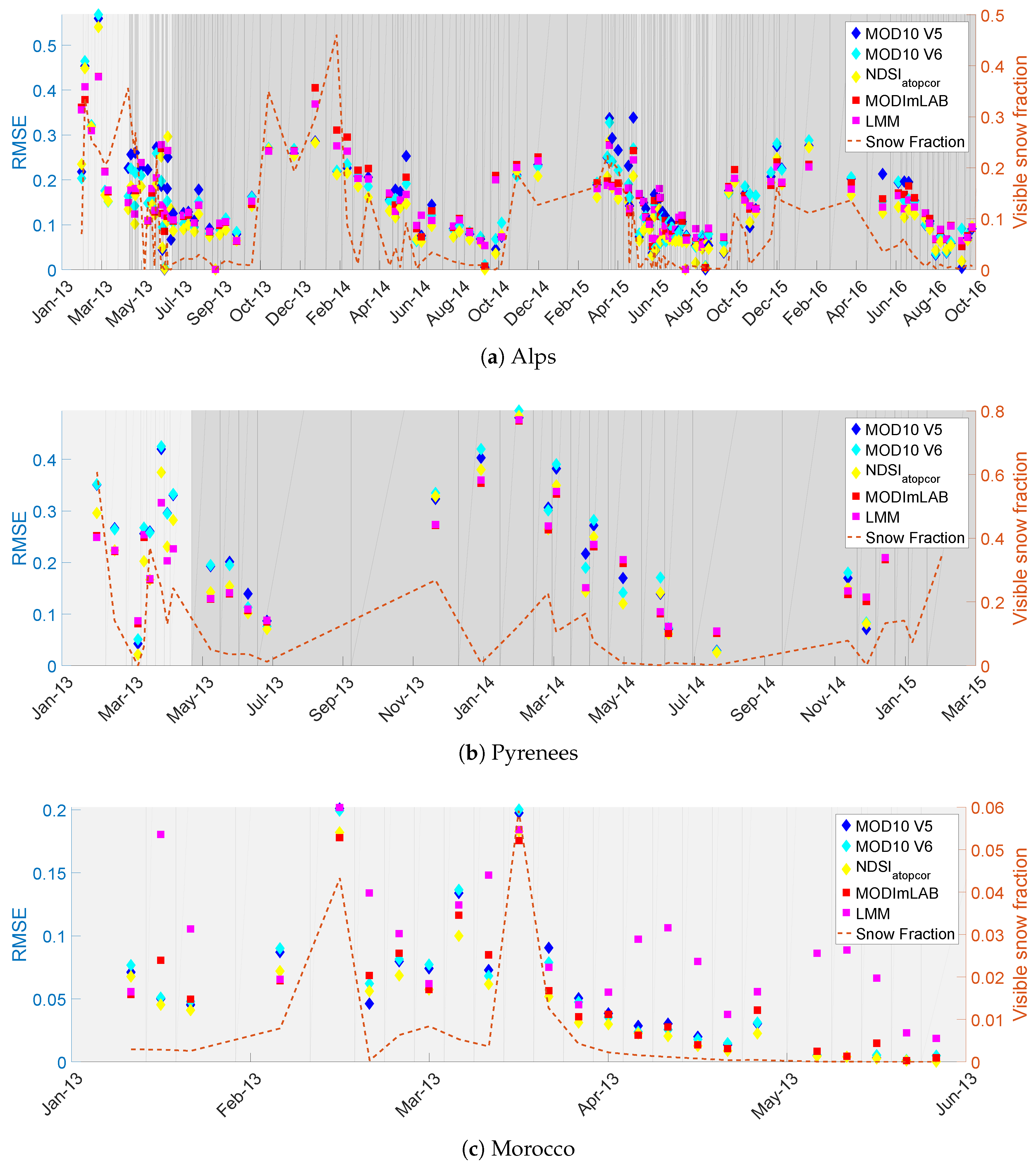
Fractional metrics allow a more precise description of errors than binary metrics since, unlike with binary metrics, a “small” error impacts the result less than a “big” error. Mean values for RMSE are presented in Table 2 and show significant variations between the different areas. However, mean values are not able to accurately describe variations in the results throughout the season. The day-by-day results for RMSE and RMSEsnow are therefore presented in Figure 3 and Figure 4.
In the Alps, the mean RMSEs for MODImLAB and LMMpure were similar (0.155 and 0.154, respectively). C5 and C6 also showed similar mean results (0.157 and 0.154, respectively), with C6 being slightly more accurate. The day-by-day results reveal that, overall, C6 was more accurate, as shown in Figure 3. The best results were obtained for NDSIATOPCOR, with a mean RMSE of 0.133. These observations are reinforced by the date-by-date comparison in Figure 3, where the two MOD10A1 collections show markedly different results, especially over the first dates being compared. As regards the linear regression of the NDSI, it can be observed that NDSIATOPCOR is more precise when using the same linear regression, which further confirms the importance of atmospheric and topographic correction. LMMpure and MODImLAB presented similar results, in contrast to the results for binary metrics. LMMpure was generally found to be less accurate than MODImLAB when the snow cover was low, and more accurate when the snow cover increased. However, the tendency of LMMpure towards producing false positives, as previously demonstrated by its low precision, did not significantly affect its RMSE.
The correlation coefficient R between these time series and the corresponding global SCF for the area (orange line) is relatively high ( 0.7 R 0.8 depending on the approach). This correlation is to be expected due to the natural decrease in the number of pixel where large errors (i.e., with a high SCF) are possible in contrast with snow-free pixels, where low false positives are minimized by the RMSE.
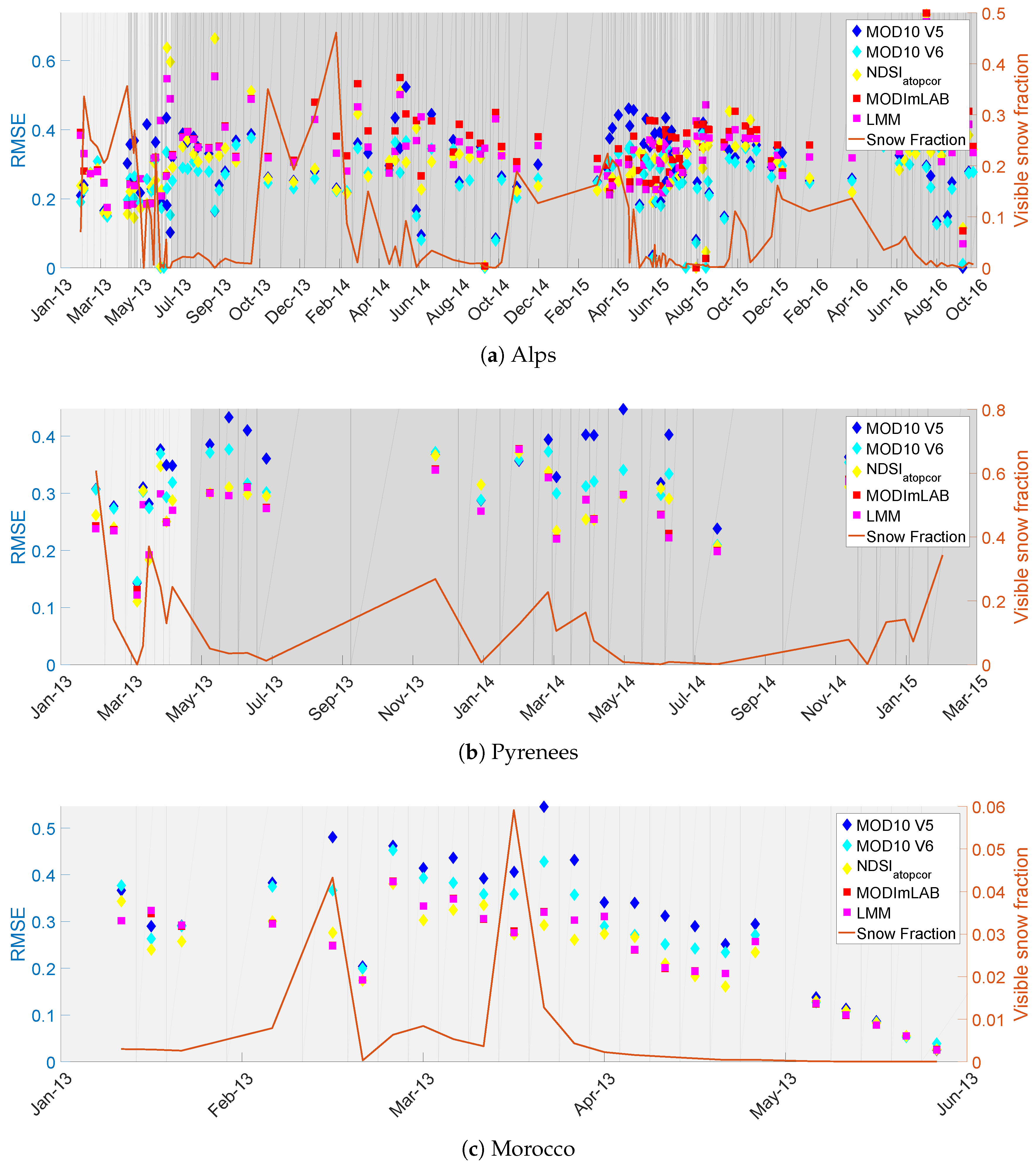
RMSEsnow (Figure 4a) shows the ability of the approach to reconstruct snow without being dependent on the global SCF. The mean results (Table 2) ranked the approaches in the same order as they did with RMSE, except for LMMpure, which was almost on a level with MODImLAB (0.233 and 0.234, respectively). This shows how well SU approaches are able to reconstruct snow. C5 was generally less accurate than the other approaches.
The error distribution showing the difference between the products and the reference (not shown here) was centered on 0 for all products. However, for LMM, the variance was higher than for the other products. In the case of C5, the error distribution was slightly non-symmetrical towards negative values, indicating a high number of snow-covered surfaces detected as snow-free. This was the main difference between C5 and C6, which no longer had this peak of snow-covered surfaces being detected as snow-free. All the products showed minor peaks around +1, indicating snow-free pixels detected as being fully covered by snow.
In the Pyrenees, the results for the NDSI approaches ranked them in the same order, but with values of between 7 and 9 points behind the Alps. NDSIATOPCOR was 3 points lower than other NDSI approaches, with a mean RMSE of 0.215 (Table 2). C6 and C5 were almost equal, with mean RMSEs of 0.246 and 0.244, respectively. For the SU approaches, MODImLAB and LMMpure produced similar results (mean RMSEs of 0.207 and 0.211, respectively). These latest results are the most accurate for this region. The correlation between the RMSE and the global snow cover fraction was less obvious ( 0.37 R 0.52 ), with substantial errors on 13 April 2013 when a low amount of snow was detected, mainly due to a high cloud cover fraction, which masked snow in open areas.
For RMSEsnow (Figure 4b), the ranking of the approaches was considerably heterogeneous. LMMpure and MODImLAB had the most accurate results although it is at an RMSE of 0.280snow, similar to the Alps.
The error distribution showing the difference between the products and the reference (not shown here) was similar to that for the Alps, although with a higher variance and a slight shift towards positive values in the case of the NDSI approaches. The rest of the error distribution was the same as for the Alps, except for the peak value at +1, which was higher, probably influenced by the larger proportion of forested areas.
In the Moroccan Atlas, the very low global fraction of snow increased both the daily and mean differences between MODImLAB and LMMpure, for which the mean RMSEs were 0.053 and 0.091, respectively. The two MOD10A1 approaches produced similar results, both having a mean RMSE of 0.057. NDSIATOPCOR was the most accurate, with an RMSE of 0.047. The correlation between the RMSE and variations in the global snow cover fraction was high (≥0.9) for all the approaches except LMMpure, which showed significant and non-correlated variations in the April–June period. These very low RMSEs were directly related to the very low global SCF. The RMSEsnow values were lower than for the Alps or Pyrenees, with a mean RMSEsnow slightly higher than 0.20 for the most accurate approaches. The results reveal that the NDSI approaches have the advantages in this area, highlighting the difference between MOD10A1 Collections 5 and 6.
The error distribution showing the difference between the products and the reference (not shown here) was similar to that for the Alps, although with a lower variance for the NDSI approaches and a higher rate of small errors for the SU approaches. The rest of the observations were the same as for the Alps, with a clear improvement in the high false positive rate in C6 compared with C5.

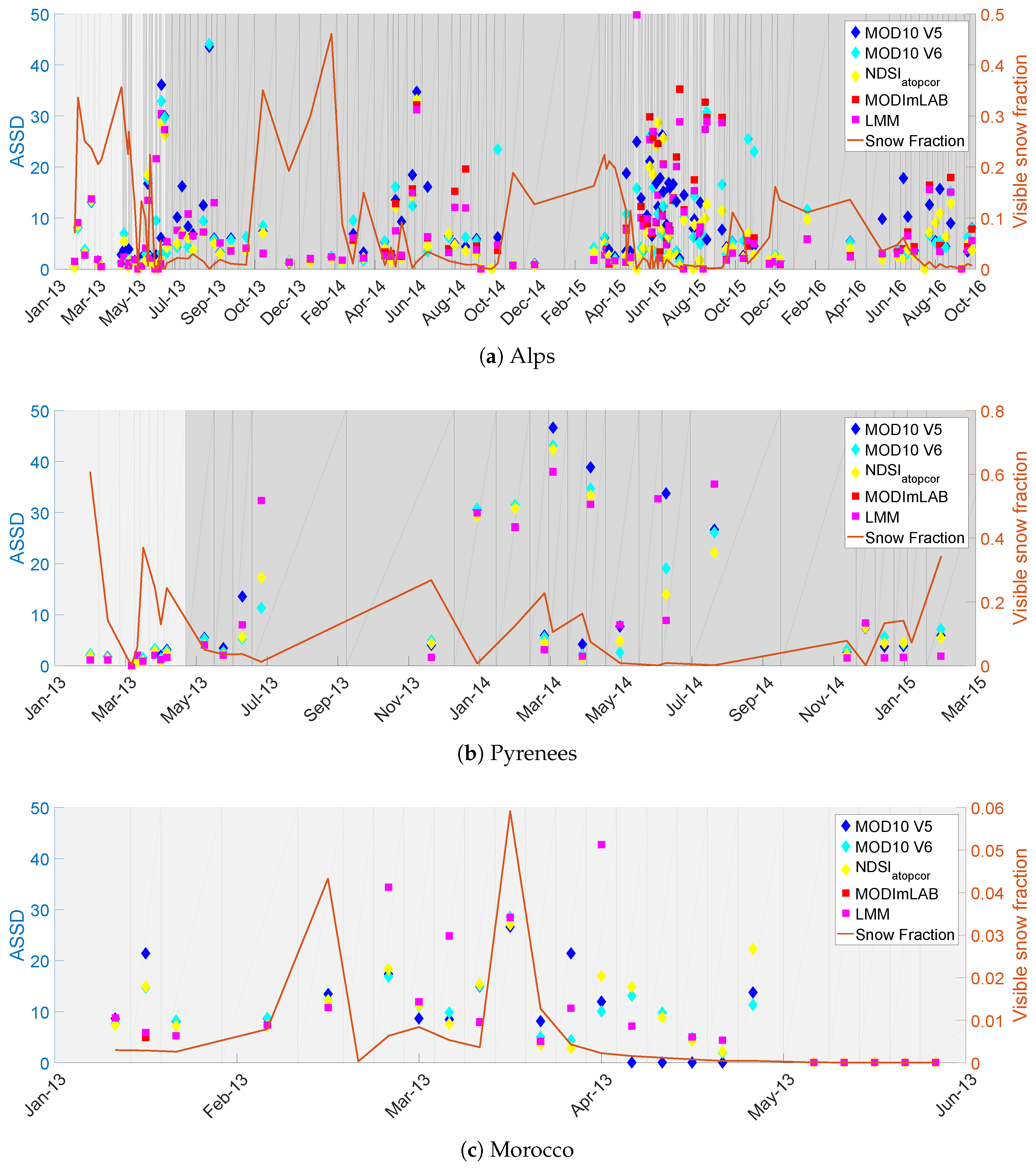
5.3. Feature-Based Metrics

In the Alps, the ASSD (Figure 5) calculated for a snow line at 50% of snow cover fraction was more accurate for the products with a native spatial resolution of 250 m. The results for MODImLAB and LMMpure were similar, though the latter are slightly more accurate than the former. Once again, C6 produced better results than C5. More generally, it can be observed that results became more divergent as the global SCF decreased.
In the Pyrenees, there was significant agreement between the different approaches, although the SU approaches still showed greater improvement. Increased ASSD values where there was low global SCA was less evident but nonetheless present.
In Morocco, the very low global SCF produced high ASSD values. The accuracy ranking of all approaches changed over the period. NDSI approaches are close, as they are for LMMpure and MODImLAB. Later dates showed very significant ASSD values, which could not be represented on the graph.

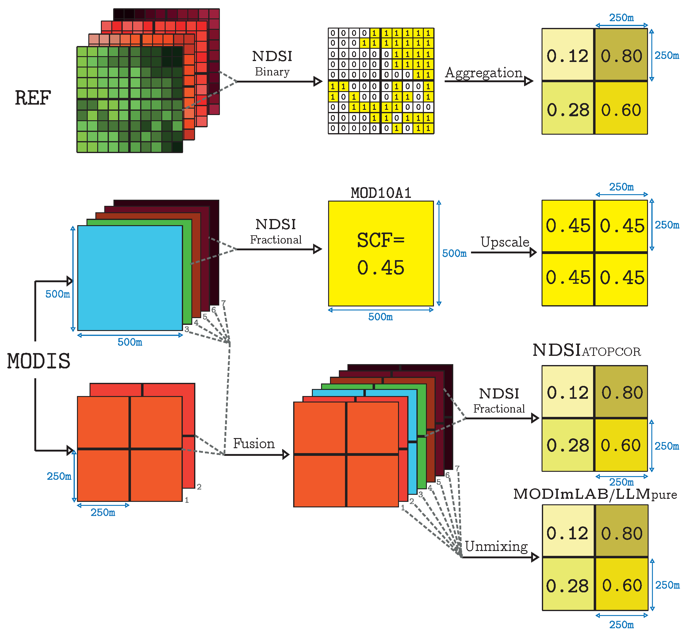
5.4. Metrics at 500 m

Products at 500 m were obtained using the same method described for the reference in Figure 2. The results are not shown here due to the high similarity between these graphs and those at 250 m. The effect was found to be identical for all areas: while fractional and binary metrics showed a slight improvement (of around 1–5 points for RMSE, for example), there was no change in the methods’ ranking. In conclusion, the pixel size used for the evaluation does not significantly influence the result. In particular, products at 500 m are not at a disadvantage compared to products at 250 m, except when it comes to the ASSD, for which the initial resolution is important.

5.5. Impact of Land Cover

The total snow cover area (SCA; i.e., the sum of the various snow fractions) for each land cover type (from the Corine Land Cover dataset) was computed and compared over the different dates in the Alps for the reference dataset and the different products. The following results are applicable to all the products (not shown here). On both natural grassland and bare rock, temporal variations in SCA were consistent. There were few differences, but the correlation coefficient was very high (≥0.99), even though the difference between the two SCA values was significant, especially on bare rock. Conversely, on land containing coniferous forest or mixed forest, there were marked differences between the reference and the products (correlation coefficients of 0.80 and 0.87, respectively), especially for dates following snowfall. This might indicate the impact of snow on the canopy and reveals the limitations of the reference. In such cases, the product seems to provide a more realistic representation of these areas than the reference.

6. Discussion

The detection of snow cover extent still suffers from significant errors and difficulties, and difficulties. As shown in this study, the two main approaches (NDSI linear regression and SU) can result in various errors, with various limitations depending both on the main approach and on the detailed workflow.
NDSI approaches are very sensitive to the initial correction of reflectance data. These results suggest that the use of accurate topographic and atmospheric correction is effective in producing more accurate results than TOA reflectance. This is particularly apparent in the Alps data, but less obvious in the Pyrenees, and less significant in terms of gain in Morocco. They also show that the changes to radiance correction in the newer MOD10A1 collection have had a considerable influence on the results (improvements in the Alps and Morocco, less conclusive in the Pyrenees). However, it is crucial to note that all comparisons using NDSI approaches were carried out using the linear regression method described in [9], which was determined on TOA reflectance in a former data collection of the sensor. If this fit produces good results in this study, an update of the value of the linear regression could be considered in the future, but would require a larger number of high-resolution dates. This would appear to be an issue for the proposed product NDSIATOPCOR, as the global results for this product were more accurate, but snow estimation was less precise than it was with C6.
The SU approaches generally produced poorer results in terms of SCF estimation, and it would seem that there is need for some improvement. This being said, the results for the SU approaches were more stable over the season compared to C5 or C6. For MODImLAB, the necessity of applying a threshold (based on the NDSI value of the pixel) was demonstrated by the results obtained for LMMpure (i.e., no thresholding). A high false positive rate was avoided by the use of a threshold, which improved the precision but decreased the recall. The effect on RMSE was minimal, since this metric minimizes small errors but can be an issue where there is sparse snow cover. The SU approaches were also limited by their design. Firstly, the computing time is higher, by about 2600 times, for an area like the Alps (7.17 s for SU versus 0.0027 s for NDSI). Secondly, in the case of MODImLAB/LMMpure, the number of endmembers is constant, designed for New Zealand and allows three types of snow, ice, and four other materials. This theoretically limits the results over Morocco, even though tests were carried out by manually adding a “sand” endmember to the process and did not improve the results.
More generally, the number of endmembers used in an SU product is limited to ensure the proper working of the algorithm. If too many endmembers are used, the results become less accurate. This has been tested by increasing the number of endmembers in the LMM products. In reality, the execution of the LMM through an FCLSU algorithm tries to include all endmembers defined in the abundance estimation of the pixel. This leads to greater numbers of errors as the number of endmembers increases. Recent alternative approaches using SU, like sparse regression [25], endmembers bundles [26,27,28], non-linear approaches [29], the perturbed linear mixing model [30], and the recent extended linear mixing model (ELMM) [31], are likely to improve the estimation of snow cover.
Typically, results and discussion focus on the global RMSE, used as the main efficiency criterion in previous studies [9,11,12]. These results show that the global RMSE is dependent on the global SCF, since errors on snow-free areas (i.e., false positives) are minimal, and do not significantly influence the global RMSE, or else can be suppressed using a threshold. The RMSE can be artificially decreased by extending the study area to include non-covered snow pixels. Conversely, for the RMSE on snow-covered surfaces (Figure 4), the SCF reconstruction errors are greater and relatively constant, allowing the limitations, and the performances, of the different approaches to be analyzed. In all cases, the goal of an RMSE of 10%, described as the objective of the NSIDC in [11], was rarely achieved, as the typical RMSEsnow values were between 0.20 and 0.35. Using RMSEsnow and ASSD metrics, compared with using RMSE alone, allowed the efficiency of the approaches to be better quantified. ASSD is also a great way of showing how the fusion process has improved snow line delimitation.
There were also considerable differences in the results found for the different areas. The ranking of the NDSI approaches in the Alps was as expected based on the complexity of the approach: the newer MOD10A1 collection was more accurate than the older one, and ATOPCOR correction outperformed both MOD10A1 collections. In the Pyrenees, these results were no longer as clear-cut, since the NDSI approaches were ranked more similarly, and often the approaches’ ranking order was reversed. Various hypotheses in regard to these differences can be made, specifically pertaining to, for example, the validity of the linear regression or the much larger proportion of forested areas in the Pyrenees compared to the Alps (Figure 1). These forest areas call into question the validity both of the product and the reference, as the definition of snow cover in these areas is not obvious.
The validity of the reference is still the main problem to overcome, as there are great uncertainties and difficulties in assessing it. The comparison of the different land covers demonstrated that uncertainties are very significant in forested regions, a problem discussed at length in [15,23]. This study has confirmed once more that snow is generally underestimated in these areas, especially when snow is present on the canopy. Below the canopy, snow is no longer visible and reaches the general limitation of optic visible detection.A simple solution could be to mask all forested areas; however, even after masking out the forested areas, the RMSE would remain larger than 10% due to errors affecting bare rock areas. The latter errors can originate from two sources: (i) the inaccurate treatment of mixed pixels in the product and (ii) the inaccurate treatment of mixed pixels in the reference. The principle of the binary reference is to “cut” the NDSI value corresponding to a certain SCF (generally 40%) to classify areas as covered by snow or not. This value can lead to errors of up to 60% for snow. While the use of small pixels statistically decreases the problem of sparse snow and sparse intruder material, it seems that snow maps at 10 m are not sufficiently pure to allow for a proper comparison. In contrast to the study by [23], a careful evaluation of the relevant dates, especially after snowfall, suggests that the errors found in the references may be greater than those of an SU product. The major limitation is still the decision of whether or not to define a mixed area with trees or shrubs covered by snow as fully covered (snow on the ground) or partly covered (visible trees).
Another approach could consist in making a fractional reference, using unmixing such as in [15] or linear regression. The main constraint would be to assess the accuracy of this reference with, e.g., a very high spatial resolution like Pleiades. Preliminary results involving non-validated products seem to show that the method used to produce the reference has an impact on the results. NDSI thresholding and NDSI linear regression require VIS and SWIR bands, which, despite being different for different satellites, have similar responses that can artificially advantage NDSI linear regression approaches. Similarly, an SU reference will use a certain number of main materials that are similar to the product, which can imply a certain similarity in the detection method and a bias in the results that cannot be quantified without the availability of a verified fractional reference. This potential bias will need to be taken into account and examined in future comparisons and assessments.

7. Conclusions

This paper presents a comparison of the two main approaches available for snow cover estimation (i.e., NDSI linear regression and linear SU), looking at five products, three using the NDSI approach ( NDSIATOPCOR and MOD10A1 C5 and C6) and two using SU (MODImLAB and LMMpure). The assessment was carried out using high-resolution snow maps taken from the SPOT 4 and SPOT 5 Take 5 experiments and LANDSAT-8 data using the Let-it-Snow chain product. Areas of comparison were identified over the French Alps, the Pyrenees, and Morocco. Binary, fractional, and feature-based metrics were used to compare the different products with the reference maps.
These results show the significant improvements of the newer MOD10A1 Collection 6 compared to the older Collection 5. However, both products were generally outperformed when using the same linear regression method but applied to atmospheric- and topographic-corrected reflectance instead of TOA reflectance. Despite the need for a threshold on NDSI or SCF values, SU approaches were found to be reliable methods, especially when estimating snow cover fraction, the results of which tended to be more stable compared with the NDSI linear regression method. The comparison uses all the products as if they were processed for a global product, i.e., without local adaptation. The scores obtained for MODImLAB are not wider spread than the scores obtained for NDSI over the three areas of interest, covering three different types of mountains. This indicates that the SU approach, such as MODImLAB, could be applied over different mountain types without a greater decrease in accuracy than NDSI. This would suggest that SU approaches are not more dependent on local adjustment than NDSI-based calculations. Low snow cover fraction and false detection (usually removed by the use of a threshold) are currently the main limitations of these approaches, which are able to better represent the variety of snow cover fractions.
Forested areas are still one of the most problematic aspects when it comes to the remote sensing of snow. While the rate of errors was significant in these areas, it seems that a proportion of the errors were also produced by the reference. This reference, computed using an NDSI approach, which is one of the more accurate approaches currently available, did not perform so well in mixed areas, which creates uncertainty over the real RMSE values of the approaches tested.
Perspectives for snow detection by improving these two approaches are numerous. NDSI linear regression produced better results when used alongside atmospheric and topographic correction, although the linear regression was defined on TOA. If a large series of verified and very accurate ground truth data were to be established, a new linear regression model could be defined. For SU approaches, new developments in endmember estimation or spectral variability could improve the original results and reduce the need for a threshold to avoid false detection.

Acknowledgments

This work has been partly supported by a grant from Labex OSUG@2020 (Investissements d’avenir—ANR10 LABX56), from the Programme National de Télédétection Spatiale (PNTS), grant n. PNTS-2016-03, the ANRJCJC EBONI, the CNES Tosca program, the OPCC CLIM’PY Interreg Programme V-A Spain-France-Andorra (POCTEFA 2014-2020) and the ARC 3 program of the Region Rhone Alpes. We would also like to acknowledge the CNES for providing the original SPOT 4 and SPOT 5 Take 5 data, and Karl Rittger for his pertinent remarks.

Author Contributions

Théo Masson wrote the paper and conceived the methodology to assess the different product available. Marie Dumont provided guidance and support throughout the research process to develop the assessment, analyze the results and wrote the paper. Simon Gascoin processed the high resolution reference images for the three areas with the LIS algorithm. Pascal Sirguey provided MODImLAB. Simon Gascoin, Pascal Sirguey and Jean-Pierre Dedieu provided advice on data analysis and pertinent analyze of the results. Marie Dumont, Mauro Dalla Mura and Jocelyn Chanussot supervised Théo Masson in the framework of his PhD and helped to discuss the results. All authors reviewed the manuscript.

Conflicts of Interest

The authors declare no conflict of interest.

References

  1. Warren, S.G. Optical properties of snow. Rev. Geophys. 1982, 20, 67–89. [Google Scholar] [CrossRef]
  2. Parajka, J.; Blöschl, G. Spatio-temporal combination of MODIS images–potential for snow cover mapping. Water Resour. Res. 2008, 44. [Google Scholar] [CrossRef]
  3. Barnes, W.L.; Pagano, T.S.; Salomonson, V.V. Prelaunch characteristics of the moderate resolution imaging spectroradiometer (MODIS) on EOS-AM1. IEEE Trans. Geosci. Remote Sens. 1998, 36, 1088–1100. [Google Scholar] [CrossRef]
  4. Justice, C.O.; Vermote, E.; Townshend, J.; Defries, R.; Roy, D.; Hall, D.; Salomonson, V.; Privette, J.; Riggs, G.; Strahler, A.; et al. The Moderate Resolution Imaging Spectroradiometer (MODIS): Land remote sensing for global change research. IEEE Trans. Geosci. Remote Sens. 1998, 36, 1228–1249. [Google Scholar] [CrossRef]
  5. Hall, D.K.; Riggs, G.A.; Salomonson, V.V. Development of methods for mapping global snow cover using moderate resolution imaging spectroradiometer data. Remote Sens. Environ. 1995, 54, 127–140. [Google Scholar] [CrossRef]
  6. Hall, D.K.; Riggs, G.A.; Salomonson, V.V.; DiGirolamo, N.E.; Bayr, K.J. MODIS snow-cover products. Remote Sens. Environ. 2002, 83, 181–194. [Google Scholar] [CrossRef]
  7. Dozier, J. Spectral signature of alpine snow cover from the Landsat Thematic Mapper. Remote Sens. Environ. 1989, 28, 9–22. [Google Scholar] [CrossRef]
  8. Salomonson, V.; Appel, I. Estimating fractional snow cover from MODIS using the normalized difference snow index. Remote Sens. Environ. 2004, 89, 351–360. [Google Scholar] [CrossRef]
  9. Salomonson, V.V.; Appel, I. Development of the Aqua MODIS NDSI fractional snow cover algorithm and validation results. IEEE Trans. Geosci. Remote Sens. 2006, 44, 1747–1756. [Google Scholar] [CrossRef]
  10. Vikhamar, D.; Solberg, R. Snow-cover mapping in forests by constrained linear spectral unmixing of MODIS data. Remote Sens. Environ. 2003, 88, 309–323. [Google Scholar] [CrossRef]
  11. Painter, T.H.; Rittger, K.; McKenzie, C.; Slaughter, P.; Davis, R.E.; Dozier, J. Retrieval of subpixel snow covered area, grain size, and albedo from MODIS. Remote Sens. Environ. 2009, 113, 868–879. [Google Scholar] [CrossRef]
  12. Sirguey, P.; Mathieu, R.; Arnaud, Y. Subpixel monitoring of the seasonal snow cover with MODIS at 250 m spatial resolution in the Southern Alps of New Zealand: Methodology and accuracy assessment. Remote Sens. Environ. 2009, 113, 160–181. [Google Scholar] [CrossRef]
  13. Bioucas-Dias, J.; Plaza, A.; Dobigeon, N.; Parente, M.; Du, Q.; Gader, P.; Chanussot, J. Hyperspectral unmixing overview: Geometrical, statistical, and sparse regression-based approaches. IEEE J. Sel. Top. Appl. Earth Obs. Remote Sens. 2012, 5, 354–379. [Google Scholar] [CrossRef]
  14. Hapke, B. Theory of Reflectance and Emittance Spectroscopy; Cambridge University Press: Cambridge, UK, 2012. [Google Scholar]
  15. Rittger, K.; Painter, T.; Dozier, J. Assessment of methods for mapping snow cover from MODIS. Adv. Water Resour. 2013, 51, 367–380. [Google Scholar] [CrossRef]
  16. Sirguey, P.; Mathieu, R.; Arnaud, Y.; Khan, M.; Chanussot, J. Improving MODIS spatial resolution for snow mapping using wavelet fusion and ARSIS concept. IEEE Geosci. Remote Sens. Lett. 2008, 5, 78–82. [Google Scholar] [CrossRef] [Green Version]
  17. Ranchin, T.; Wald, L. Fusion of high spatial and spectral resolution images: the ARSIS concept and its implementation. Photogramm. Eng. Remote Sens. 2000, 66, 49–61. [Google Scholar]
  18. Nolin, A.; Liang, S. Progress in bidirectional reflectance modeling and applications for surface particulate media: Snow and soils. Remote Sens. Rev. 2000, 18, 307–342. [Google Scholar] [CrossRef]
  19. Riggs, G.A.; Hall, D.K.; Román, M.O. Overview of NASA’s MODIS and VIIRS Snow-Cover Earth System Data Records. Earth Syst. Sci. Data Discuss. 2017, 2017, 1–30. [Google Scholar] [CrossRef]
  20. Feranec, J.; Soukup, T.; Hazeu, G.; Jaffrain, G. European Landscape Dynamics: CORINE Land Cover Data; CRC Press: Boca Raton, FL, USA, 2016. [Google Scholar]
  21. Channan, S.; Collins, K.; Emanuel, W. Global Mosaics of the Standard MODIS Land Cover Type Data; University of Maryland and the Pacific Northwest National Laboratory: College Park, MD, USA, 2014; Volume 30. [Google Scholar]
  22. Dong, J.; Peters-Lidard, C. On the relationship between temperature and MODIS snow cover retrieval errors in the Western US. IEEE J. Sel. Top. Appl. Earth Obs. Remote Sens. 2010, 3, 132–140. [Google Scholar] [CrossRef]
  23. Gascoin, S.; Hagolle, O.; Huc, M.; Jarlan, L.; Dejoux, J.F.; Szczypta, C.; Marti, R.; Sánchez, R. A snow cover climatology for the Pyrenees from MODIS snow products. Hydrol. Earth Syst. Sci. 2015, 19, 2337. [Google Scholar] [CrossRef] [Green Version]
  24. Heimann, T.; Van Ginneken, B.; Styner, M.; Arzhaeva, Y.; Aurich, V.; Bauer, C.; Beck, A.; Becker, C.; Beichel, R.; Bekes, G.; et al. Comparison and evaluation of methods for liver segmentation from CT datasets. IEEE Trans. Med. Imaging 2009, 28, 1251–1265. [Google Scholar] [CrossRef] [PubMed]
  25. Iordache, M.D.; Plaza, A.; Bioucas-Dias, J. On the use of spectral libraries to perform sparse unmixing of hyperspectral data. In Proceedings of the 2010 2nd Workshop on Hyperspectral Image and Signal Processing: Evolution in Remote Sensing, Reykjavik, Iceland, 14–16 June 2010; pp. 1–4. [Google Scholar]
  26. Somers, B.; Zortea, M.; Plaza, A.; Asner, G.P. Automated extraction of image-based endmember bundles for improved spectral unmixing. IEEE J. Sel. Top. Appl. Earth Obs. Remote Sens. 2012, 5, 396–408. [Google Scholar] [CrossRef]
  27. Zare, A.; Ho, K. Endmember variability in hyperspectral analysis: Addressing spectral variability during spectral unmixing. IEEE Signal Process. Mag. 2014, 31, 95–104. [Google Scholar] [CrossRef]
  28. Jin, J.; Wang, B.; Zhang, L. A novel approach based on fisher discriminant null space for decomposition of mixed pixels in hyperspectral imagery. IEEE Geosci. Remote Sens. Lett. 2010, 7, 699–703. [Google Scholar] [CrossRef]
  29. Heylen, R.; Burazerovic, D.; Scheunders, P. Non-linear spectral unmixing by geodesic simplex volume maximization. IEEE J. Sel. Top. Signal Proc. 2011, 5, 534–542. [Google Scholar] [CrossRef]
  30. Thouvenin, P.A.; Dobigeon, N.; Tourneret, J.Y. Hyperspectral unmixing with spectral variability using a perturbed linear mixing model. IEEE Trans. Signal Proc. 2016, 64, 525–538. [Google Scholar] [CrossRef]
  31. Drumetz, L.; Henrot, S.; Veganzones, M.A.; Chanussot, J.; Jutten, C. Blind hyperspectral unmixing using an Extended Linear Mixing Model to address spectral variability. In Proceedings of the 7th Workshop on Hyperspectral Image and Signal Processing: Evolution in Remote Sensing (WHISPERS 2015), Tokyo, Japan, 2–5 June 2015. [Google Scholar]
Figure 1. The three areas of interest in the French Alps (a), the Pyrenees (b), and the Moroccan Atlas (c). The land cover types for the Alps and Pyrenees shown to the right of the figure are from the Corine Land Cover library [20] at a spatial resolution of 30 m. Land cover for Morocco was obtained from classification of MODIS using imagery at a spatial resolution of 500 m from [21].
Remotesensing 10 00619 g001
Figure 2. Workflow of the methodology used in this study to produce comparable maps of SCF at 250 m. The top line describes the aggregation methodology for the reference snow maps initially based on NDSI thresholding. The other lines details the methodology for the different products from MODIS data: from two of the five 500 m bands of MODIS for the MOD10A1 (based on NDSI linear regression) products at 500 m upscaled to 250 m (middle line), the seven fused bands of MODIS for MODImLAB and LMMpure (based on unmixing), and two of these fused bands for NDSIATOPCOR (based on NDSI linear regression) (bottom line).
Remotesensing 10 00619 g002
Figure 3. Root mean square error (RMSE) (markers) and total snow cover fraction (orange line) over all non-cloudy pixels over the Alps (a), Pyrenees (b), and Moroccan Atlas (c), as a function of all the available dates in each area. Square markers represent SU approaches and diamond-shaped markers represent NDSI approaches. The color of the background corresponds to the sensor used as reference. The lighter grey represents SPOT 4, the medium grey SPOT 5, and the darker grey LANDSAT-8.
Remotesensing 10 00619 g003
Figure 4. Total snow cover fraction (orange line) and RMSE (markers) for snow-covered and non-cloudy pixels only (RMSEsnow), over the Alps (a), Pyrenees (b), and Moroccan Atlas (c), as a function of all the available dates in each area. Square markers represent SU approaches and the diamond-shaped markers NDSI approaches. The color of the background corresponds to the sensor used as reference. The lighter grey represents SPOT 4, the medium grey SPOT 5, and the darker grey LANDSAT-8.
Remotesensing 10 00619 g004
Figure 5. Average symmetric surface distance (ASSD) of the snow line at 50% threshold (markers) and global snow cover fraction (orange line) for the Alps (a), Pyrenees (b), and Moroccan Atlas (c) as a function of available dates in each area. The most recent dates could not be plotted for Morocco due to the SCA being too low. Square markers correspond to SU approaches and diamond-shaped markers to the NDSI approaches. The color of the background corresponds to the sensor used as reference. The lighter grey represents SPOT 4, the medium grey SPOT 5, and the darker grey LANDSAT-8.
Remotesensing 10 00619 g005
Table 1. Main characteristics of the three areas studied.
Size (km 2 )DatesMin. AltitudeMax. Altitude
French Alps92161172004100
Pyrenees12,100302503300
Atlas14,625241004080
Table 2. Average binary and fractional metrics values for the three areas of interest compared at 250 m (range [0–1]). An efficient approach will show high scores for binary metrics (Fscore, Precision, and Recall) and low values for RMSE and RMSEsnow.
ZoneMethodFscorePrecisionRecallRMSERMSEsnow
AlpsC50.4740.6710.4720.1570.286
C60.5060.4670.6620.1540.250
NDSIATOPCOR0.6410.7050.6610.1330.303
MODImLAB0.5000.5590.5950.1550.347
LMMpure0.3400.2600.8120.1540.335
PyreneesC50.5860.6540.6770.2440.320
C60.5920.5090.7960.2460.312
NDSIATOPCOR0.6700.6520.7740.2150.290
MODImLAB0.6200.5230.8900.2070.280
LMMpure0.4620.3570.9500.2110.279
MoroccoC50.2370.4890.2160.0570.306
C60.3920.4210.4230.0570.274
NDSIATOPCOR0.4460.6230.4210.0470.228
MODImLAB0.4520.4080.6230.0530.236
LMMpure0.0690.0380.7090.0910.236

