1. Introduction

This paper deals with the measurement of crystal orientation fabric and crystal area from ice thin sections. Standard thin-section measurements lead to orientation densities in terms of the percentage of individual crystals having various orientations. Reference KambKamb (1959) suggested, however, that interpretation of the observed fabric patterns should logically deal with the relative volume of the various orientations in the polycrystal. Reference KambKamb (1959) used the Schmidt equal-area projection point diagram not only to show the orientation of each crystal measured, but also to indicate its approximate area. He replaced the classical point of one orientation on the Schmidt diagram by three symbols which indicated three different classes of grain area. Because only a few, larger, grains were measured manually, Kamb’s proposition did not become the Schmidt diagram standard.

The use of some statistical parameters, such as the strength of fabric or the orientation tensor (defined in Equation (10)), seems to complement the Schmidt diagrams, as it gives a more quantitative description of the different fabric patterns. Using automatic instruments for fabric and texture measurements on ice, it is easy to measure the cross-sectional area of all the grains at the same time as their orientation (Reference Wang and AzumaWang and Azuma, 1999; Reference WilenWilen, 2000). Therefore, following the idea of Reference KambKamb (1959), it seems natural to use the area measured on the thin section as a statistical weighting of the individual crystals. Note that in materials science, fabric is traditionally defined in this manner, due to the automatic texture measurements developed earlier (Reference KambKocks and others, 1959).

During the last 10 years, considerable effort has been devoted to the modelling of fabric evolution and induced anisotropy of polycrystalline ice (Reference Azuma and Goto-AzumaAzuma and Goto-Azuma, 1996; Reference Meyssonnier and PhilipMeyssonnier and Philip, 1996; Reference CastelnauCastelnau and others, 1998; Reference Montagnat and DuvalMontagnat and Duval, 2000). Models relating micro-structure to macroscopic behaviour have been developed and have been used to reproduce the observed fabric in some polar ice cores (Reference CastelnauCastelnau and others, 1998; Reference Montagnat and DuvalMontagnat and Duval, 2000). Since the strain rates in polar ice are very low, laboratory tests are not possible and the only way to validate such models is to compare modelled and observed fabrics by considering statistical parameters. Therefore, one must try to obtain from the two-dimensional (2-D) thin-section measurements the best description of the actual ice fabric. We will show that the fabric description can be improved by using the measured cross-sectional area of the grain to infer its volume fraction.

The main assumption introduced is that the grain volume can be determined from the measurement of the 2-D grain area, i.e. that the measured cross-sectional area is the mean projected area of the grain. The bias introduced by this assumption is difficult to quantify. For a polydispersed system of spheres, Reference UnderwoodUnderwood (1970) solved the backward problem to pass from the distribution of a 2-D section to the distribution of three-dimensional (3-D) spheres, by performing the stereological transformation

where is the number of grains having a diameter determined from grain volume in size class j and D_j is the diameter determined from volume for size class j. The sum , which represents the number per unit area of sections in class size i obtained from spheres of all possible sizes, is a directly measurable quantity. The probability P_i,j of a thin section intersecting a sphere of diameter j to yield sections of diameter i can be calculated analytically for a poly-dispersed system of spheres (Reference UnderwoodUnderwood, 1970). Using Equation (1) and 3-D computer simulations of grain growth, Reference Anderson, Grest and SrolovitzAnderson and others (1989) showed that the grain-size distribution obtained from the grain volume can be inferred with excellent agreement with that obtained from 2-D area measurements when using a probability function P_ij derived for the pentagonal dodecahedron instead of the sphere. Reference Gay and WeissGay and Weiss (1999) argued that the most exact method to derive true 3-D grain-growth kinetics from thin-section analyses is to measure the exact (cross-sectional) area of all the grains within the thin section.

For fabric measurements, we need to consider orientations as well as grain-size. The actual volume of each isolated grain cannot be determined from its 2-D area measurement: for example, a plane section can intersect the centre of a small grain, yielding an apparently large grain, and the tip of a large grain, yielding an apparently smaller grain (Reference Anderson, Grest and SrolovitzAnderson and others, 1989). As suggested by Reference UnderwoodUnderwood (1970), there is a higher probability that a large area represents a large grain than that a small area represents a small grain. The probability density function P(D) (the continuous form of P_i;j in Equation (1)) can be calculated for most of the theoretical grain shapes as a function of the ratio D/D_max of the diameter D observed in the cross-section to the diameter D_max of the volume. As shown by Reference Anderson, Grest and SrolovitzAnderson and others (1989), P(D) is non-uniform and shows a peak value for 0.8 <D/D _max <1. From this statistical result, one would expect a better description of the actual fabric by using area weighting instead of equal weighting.

This paper explores the use of grain area to infer the volume fraction it represents in the whole polycrystal sample. First, using a 3-D Potts model, a numerical 3-D polycrystal is built and the area weighting is compared to the actual volume fraction. Then, using both numerically simulated and natural fabrics, we give some order of magnitude of the influence on the fabric description of an area weighting instead of an equal weighting. To conclude, we discuss the pertinence of using the measured cross-sectional area of the grain for a volume-fraction definition.

2. Volume-Fraction Definitions

In what follows, three different definitions of the volume-fraction distribution , where k = 1..N, are compared: the actual volume-weighted fraction distribution , the equal-weighted volume-fraction distribution and the area-weighted volume-fraction distribution .

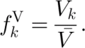
The actual volume-weighted fraction

of grain number k is defined as its volume V_k over the whole volume

occupied by the N grains of the polycrystal. We can then define the actual volume-weighted (VW) fraction by

The volume cannot be measured using thin sections. The simplest and most commonly used solution is then to assume that all the grains represent the same volume fraction, that is to use an equal-weighted (EW) volume fraction defined by

Another solution, explored in the present paper, is to assume that the volume fraction of a crystal is a function of its cross-sectional area fraction measured on the thin section. Then, the area-weighted (AW) volume fraction should be written

where A _k is the cross-sectional area of the crystal k and α is an exponent. If the measured grain area in the thin section is the mean projected area of the grain, we should have the following relationship:

where β is a coefficient that is a function of the grain shape. For example, for a sphere, and β = 0.653 for a truncated octahedron (Reference UnderwoodUnderwood, 1970, p. 90). In the next section, we study the sensitivity of the area weighting to the exponent α and try to find an optimal value for this exponent. Note that the coefficient β disappears from the definition of the area weighting and when α = 0 Equation (4) reduces to the equal weighting (Equation (3)).

By definition, each of the three volume-fraction distributions VW (Equation (2)), EW(Equation (3)) and AW (Equation (4)) verifies the following inequalities and equation:

where b is V, 0 or α, respectively.

3. Potts Model

To compare the constant and measurable volume-fraction distributions (Equations (3) and (4) respectively) to the actual distribution (Equation (2)), a 3-D microstructure is needed. Unfortunately, this kind of measurement cannot be made; only a model can give the relevant information. In the upper part of an ice sheet, the microstructure evolution is governed by the normal grain-growth process (Reference Duval and LoriusDuval and Lorius, 1980). Reference Anderson, Grest and SrolovitzAnderson and others (1989) showed that a 3-D Potts model (Reference PottsPotts, 1952) properly reproduces the topological, kinetic, grain-size distribution and morphological features of normal grain growth. In this model, the microstructure is mapped onto a 3-D cubic lattice.

Also, contiguous voxels with the same label indicate a single grain whereas a grain boundary lies between voxels with different labels. Note that the number of grains in the whole cube is much larger than the number of labels, since two different grains, as long as they are not neighbours, can have the same label. The time calculation increases with the number of labels, and for the present application we choose 324 possible labels. This choice is in agreement with Reference Anderson, Grest and SrolovitzAnderson and others (1989), who argued that this number must be large enough (>48) to avoid impingement of grains having the same label.

The driving force for grain growth in polycrystalline materials is the decrease of the total grain boundary energy within the material (Reference RalphRalph, 1990). In the Potts model, the grain boundary energy is defined in terms of the lattice voxel energy

where J is a positive constant, S _i corresponds to the label of the lattice i, δ is the Kronecker delta, and the summation is made until the third-order neighbour, i.e. for p = 3 and N _p = 26. The kinetic of the boundary motion is simulated by a Monte Carlo technique. A voxel is randomly selected, and then a new label number for this voxel is randomly sampled over the 324 possibilities. Then the change in energy linked to this new label is calculated according to Equation (7). Only new labels giving ΔE< 0 are accepted.

For the application, the polycrystal is a cube of 400 pixels on each side and the grain growth evolution is stopped when the mean grain area over the horizontal 400 cross-sections is similar to that observed in natural thin sections (approximately 300 grains in a thin section). Assuming the shapes of the modelled grains are similar to those of a natural ice sample, one should expect from these results an objective comparison of the three definitions of the volume fraction. Note that results for the intermediate steps, with more grains in each cross-section, are similar to those presented in this paper.

In what follows, just as for a natural ice thin section, the grains that intersect a boundary of the cube are discounted. Only the 301 central cross-sections (from 50 to 350) are studied and, on those, only the grains which are not cut by the boundary. The average number of non-intersecting grains per cross-section is 218, with a minimum of 179 and a maximum of 259. There is a total of 2784 non-intersecting grains in the 301 studied cross-sections.

4. Comparison of the Volume-Fraction Definitions

In each cross-section, we calculate the relative error of the volume-fraction distribution, defined by

where N _s is the number of grains in the cross-section, is one of the two volume-fraction distributions EW (Equation (3)) or AW (Equation (4)) and is the actual volume fraction VW (Equation (2)).

Using the AW distribution (Equation (4)), the minimization of the relative error (Equation (8)) as a function of the exponent α allows the calculation of the optimal value α_opt in each cross-section. As shown in Figure 1, the optimal value for the exponent α varies from 1.55 to 1.97, with an average of 1.7 over the 301 cross-sections. For all the cross-sections, the optimal value is greater than the theoretical value of 3/2. In this simulation, the grain shape is isotropic and we have verified that the results for the average of the optimal exponent α_opt are identical, whatever the direction of the cross-sections.

Fig. 1. Variation over the 301 cross-sections of the optimal value of the exponent in Equation (4) that minimizes the relative error (Equation (8)). The line represents the average of α_opt for the cross-sections.

Due to the large deformations undergone by polar ice, the shape of crystals is not isotropic since they usually flatten out as the depth increases (Reference Gay and WeissGay and Weiss, 1999). Therefore, one should expect to obtain different values of the optimal exponent α_opt from vertical and horizontal thin sections. Grains which have larger dimensions in the horizontal plane than in the vertical plane will, on average, overestimate the volume fraction determined by the area measurements in a horizontal thin section, and underestimate it for a vertical thin section.

Figure 2 shows the variation of the relative error (Equation (8)) over the 301 cross-sections for the EW (Equation (3)) and the AW (Equation (4)) with α = _opt, α = 3/2 and α = 1.0. The average of the relative error over the 301 cross-sections of the AW is 59%, 63% and 109% for α = α_opt, α = 3/2 and α = 1.0 respectively. This large error of about 60% must be compared to 1100% obtained for the EW, which is approximately 18 times larger. As shown in Figure 2, the variation of the relative error for the AW is relatively constant, with a standard deviation of 4.5% for α_opt and 6.0% for α = 3/2. For the EW, the standard deviation of the relative error is much larger (100%) and some peaks are seen on the curve. These are due to the presence of a few very small (in volume) grains in the cross-section leading to a very large error for those grains. If we exclude these very small grains, by neglecting those with a volume >64 pixels³, then the average relative error over the 301 sections decreases to 510%, still eight times larger than that obtained for the AW with α = 3/2. Note that neglecting these small grains does not affect the relative error obtained for the AW since the actual volume fraction of a small (in volume) grain is well approximated by its area weighting.

Fig. 2. Variation over the 301 cross-sections of the relative error Φ(f _k ) for the AW distribution (Equation (4)) α = α_opt (thick solid line), α= 3/2 (solid line), α = 1.0 (dotted line) and the EWdistribution (Equation (3)) (dashed lines). For the thick dashed line, the smallest grains (volume <64 pixels) have been neglected for the calculation of .

On the other hand, as shown in Figure 3 for the cross-section number 200, we verify that the smaller the area of the grain the more uncertain is the volume-fraction estimate using the AW (Equation (4)). One way of reducing the relative error (Equation (8)) should be to neglect the smallest grains in the cross-section. If the grains for which the area is <1% of the maximum area in the cross-section are neglected, the main relative error (Equation (8)) decreases from 63% to 55% for α = 3/2. If we neglect grains with area <10% of the maximum area the error is 37%, but for each of the 301 cross-sections the number of studied grains is then lower than half the total number of non-intersecting grains.

Fig. 3. Relation between the actual volume fraction (Equation (2)) and the AW fraction (Equation (4)) with α = 3/2 (circles) and the EW fraction (Equation (3)) (crosses) for the grains of the cross-section number 200. The line represents the equality . This figure looks similar for all the cross-sections.

It is then necessary to choose a percentage value below which the smallest grains are neglected, with a compromise between the number of grains studied and the accuracy of their area providing a good approximation of the volume fraction. Nevertheless, the mean relative error is still very large and, for simplicity, one should use all the measurable areas. On the cross-section number 200, about 2% of the grains have an area < 4 pixels, and they would certainly not have been measured in a real ice thin section. Figure 3 also shows the equal compared to the actual volume-fraction distribution.

According to these first results, the relative error on the volume fraction estimated by the area measurements is large (approximately 60%), but it is more than one order of magnitude lower than that obtained using EW. For this simulation, the value of the optimal exponent α is found to be about 1.7, but as shown previously, the theoretical value α = 3/2 leads to similar results. In what follows, the value of the exponent α is fixed at its theoretical value α = 3/2 and we now study the influence of the area weighting on the fabric description.

5. Influence on Fabric Description

The fabric of a polycrystal consisting of N crystals is defined by the N orientations of its grains weighted by the volume fraction that they occupy in the whole polycrystal. Since the ice single crystal is hexagonally symmetric about its c axis, its orientation in space can be described by using only the c-axis unit vector c^k, perpendicular to the crystal basal plane.

The direction of the c-axis unit vector is defined by two angles in the global reference frame {R} linked to the polycrystal (or to the thin section): the colatitude θ_k and the longitude ϕ_k. The definition of c^k in the fixed reference frame {R} is given by

where () ^T denotes the transpose.

Using the above notation, the fabric of a sample is defined in terms of the N c-axis orientations (c^k) and the N volume fractions (). In what follows, a fabric will be denoted AW, EW or VW fabric when is determined using from Equation (3), from Equation (4) or the actual weighting from Equation (2), respectively.

In the present study, we compare the results obtained from two categories of fabrics.

Figure 4 shows the Schmidt diagrams of the eight North-GRIP fabrics. The area of the circles on the Schmidt diagrams is proportional to the measured cross-sectional area of the grains. The eight NorthGRIP fabrics cover a large range of types: quasi-random (depth 148 m), girdle-type (depth 2040 m), equal girdle and cluster tendencies (depths 1328, 1873 and 2396 m) and cluster-type (depths 806, 2633 and 2840 m). From these measurements, both the orientation and the area of approximately 200 crystals were determined. In order to estimate the pertinence of the grain-size as a weight, we now compare the results obtained with equal weights (Equation (3)) and area weights (Equation (4)).

Fig. 4. Schmidt diagrams of eight NorthGRIP fabrics. The circle area is proportional to the corresponding cross-sectional grain area.

As suggested by Reference WoodcockWoodcock (1977), a good way to characterize the essential features of an orientation distribution is to use the orientation tensor a ^b defined as:

where b is either V, 3/2 or 0 and c ^k is given by Equation (9). In the symmetry reference frame, a^b is a diagonal matrix whose diagonal non-zero terms are the three eigenvalues. The three base vectors of this symmetry reference frame are the eigenvectors of a ^b. Note that the number of grains N in Equation (10) is the number of grains in a given cross-section, and only for b = V can it be the total number of grains in the whole polycrystal. In the latter case, the orientation tensor will be noted , which is the actual orientation tensor of the whole polycrystal (all the non-intersecting grains).

In what follows, the different fabrics are compared using the orientation tensor defined by Equation (10). In each of the 301 cross-sections, we define the absolute error tensor Ψ

where N _s is the number of grains in a cross-section and f^[ _k is one of the two volume-fraction distributions (Equation (4) or (3)). Each component of Ψ in Equation (11) corresponds to the absolute difference on the same component between the orientation tensor calculated using the volume-weighted fabric in the cross-section and that using either the AW or the EW fabric.

For the first category of fabrics, we built two sets of 1000 random simulations of the c-axis orientations by imposing fixed values of the orientation tensor components calculated for the whole polycrystal: a fabric with (termed the isotropic fabric set) and a fabric with a preferential orientation (termed the anisotropic fabric set). For both sets, the non-diagonal terms of are equal to zero and therefore the diagonal terms are the eigenvalues with .

From a technical point of view, the calculation of the orientations to obtain the desired orientation tensor is done by first initializing them with a random distribution, and then moving them such that the difference between the desired and the calculated orientation tensors is minimum. That is, find the distribution (θ _k ψ _k ) which minimizes

where are the components of the imposed orientation tensor and the components of the calculated orientation tensor defined by Equation (10). This minimization problem is solved by using the conjugate gradient method.

Figure 5 shows the evolution of the diagonal terms of the orientation tensor (Equation (10)) over the 301 cross-sections for the VW, AW and EW fabrics for one particular random simulation of the isotropic and anisotropic fabric sets. As shown in Figure 5a, for the isotropic fabric, it is not possible to distinguish clearly which of the two volume fractions (Equation (3) or (4)) best approximates the actual volume fraction (Equation (2)). Even if, on average over the 301 cross-sections, the norm of the absolute error tensor (Equation (11)) is 0.14 for the AW fabric and 0.20 for the EW fabric, the difference between the AW and the EW volume fractions cannot be ascertained.

Fig. 5. Variation over the 301 cross-sections of the diagonal terms of the orientation tensor for the VW fabric a^V (thick line), the AW fabric a^3/2 (solid line) and the EW fabric a⁰ (dashed line).The straight lines represent the value of the actual orientation tensor a^V calculated on the whole polycrystal. The results are presented for one particular simulation of the isotropic fabric set (a) and the anisotropic fabric set (b) .

However, for the anisotropic fabric, according to the diagonal terms of the orientation tensor, the AW fabric is clearly closer to the actual fabric. For this simulation of the c-axis orientations, on average over the 301 cross-sections, the norm of the absolute error tensor (Equation (11)) is 0.15 for the AW fabric and 0.32 for the EW fabric.

Curves for the AW fabric are smoother than for the EW and VW fabrics. This can be explained by the fact that for one grain the volume fraction varies continuously as a function of the cross-section number when it is defined using the AW, whereas it is almost constant for both EW and VW, inducing a discontinuity in the first cross-section where the grain appears.

Note that the non-diagonal terms (not plotted) of the orientation tensor for the three volume-fraction definitions are very close, but not equal, to zero. The error on these terms is implicitly taken into account when plotting the norm of the error tensor.

Since the results presented above depend on a random simulation of the c-axis orientations, one should perform many simulations of the orientations to obtain an adequate statistical treatment of the results. Figure 6 presents the probability distributions of the diagonal terms and the norm of the absolute error tensor (Equation (11)) for the 1000 simulations of c-axis orientations of the isotropic and anisotropic fabrics. As shown previously, for isotropic fabrics the AW distribution gives a better estimation of the actual fabric than the EW distribution. For the anisotropic fabric set, the distribution of the absolute error is clearly better for the AW fabric than for the EW fabric. For all the data (1000 simulations and 301 sections, i.e. 301000 in all), the average of the norm of the absolute error tensor (Equation (11)) for the EW fraction is 3.2 times larger than that of the AW fraction. As shown in Figure 6, for the isotropic set, the probability distributions of the three diagonal terms are similar, whereas for the anisotropic set they are different for both the AW and EW fabrics, depending on the value of the imposed terms .

Fig. 6. Cumulative probability distributions of the diagonal terms and the norm of the absolute error tensor (Equation (11)) for the AW fabrics (solid lines) and the EW fabrics (dashed lines).The results for two sets of simulations of the c-axis orientations are represented: isotropic set defined by (thin lines), and anisotropic set defined by (thick lines).The number of data for each set is then 1000 simulations × 301 cross-sections.

Table 1 presents the average values of the diagonal terms of the orientation tensor taken over the 1000 simulations and the 301 sections. The values obtained with the AW fraction are close to the actual values, whereas the EW fraction results are significantly different, especially when the fabric is not isotropic. Since observed fabrics are mostly anisotropic, one should expect such differences for natural fabrics measured in ice cores from Antarctica and Greenland.

Table 1. Average of the orientation tensor diagonal terms for the 1000 simulations of the isotropic set defined by and the anisotropic set defined by

Note that it would be expected that the average of the orientation tensor over the 301 cross-sections 〈a ^V 〉 is not exactly equal to that imposed for the whole polycrystal . Since the large grains appear in more cross-sections than the small grains, they are counted more often when performing the average over the 301 cross-sections.

In order to quantify how the error evolves with the fabric, the error tensor (Equation (11)) was calculated on a grid of the possible values of , i.e. on the domain . At each grid-point, 50 random simulations of the c-axis orientations corresponding to the values of the at that point were performed. Then, at each gridpoint, we calculated the average of the error tensor over the 50 simulations and the 301 cross-sections. We verified that 50 simulations are enough to obtain a good approximation of the average value of the error tensor.

Figure 7 presents the isolines of the average of the norm of the error tensor (Equation (11)) for both the AW and EW fabrics. As observed in the previous results, the difference between the two errors is lower for the isotropic fabric, i.e. for = 1/3 (no sum), but for the AW fabric it corresponds to the absolute maximum error whereas for the EW fabric it is found to be a local minimum. Note that, as shown in Figure 6, this minimum local error is still larger than the absolute maximum error for the AW fabric. More generally, for any fabrics, it is found that the absolute error for the EW fabric is, on average, 2.5 times larger than that for the AW fabric and, statistically, the AW fabric is closer to the actual fabric than is the EW fabric.

Fig. 7. Isolines of the average of the absolute error tensor norm (Equation (11)) for the AW fabrics (a) and the EW fabrics (b) as a function of . The average for one point is done over 50 simulations of the orientations times the 301 cross-sections.

Note that where one of the is equal to 1 and the two others are equal to zero, both errors are equal to zero, i.e. all the volume-fraction definitions give the same results. This is because this case does correspond to a fabric where all the grains have the same orientation.

From the eight NorthGRIP fabrics, one should expect to quantify the difference between EW and AW of natural fabrics. Following Reference KizakiKizaki (1969) and Reference Vallon, Petit and FabreVallon and others (1976) we tried to find some correlations between the grain-sizes and their orientations. For the eight NorthGRIP data, we did not observe any correlation, contrary to what had been observed by Reference Vallon, Petit and FabreVallon and others (1976) for ice in temperate glaciers. This may be because not all the grains on the thin section, but only about 200, were measured. A second explanation for the lack of correlation is that the recrystallization phenomena, which could explain such correlation between size and orientation, play a much more significant role in temperate than in cold glaciers.

Nevertheless, these NorthGRIP samples should give some idea of the quantitative influence of the grain-size on the fabric characteristics. Figure 8 shows the evolution with depth of the six terms of the orientation tensor (Equation (10)) for the AW and EW fabrics. The maximum absolute difference between the AW and EW definitions is about 0.1, and the average difference for the eight fabrics and the six terms is 0.03. One must remember that the terms of the orientation tensor are close to 1 (the eigenvalues of the tensor are between 0 and 1), and from these results one may conclude that the use of the AW can lead to significant differences (10%) compared to the classical EW.

Fig. 8. Variation with depth of the components of the orientation tensor for the AW a^3/2 (◯) and the EW a⁰ (□) fabrics measured in the NorthGRIP ice core.

6. Conclusion

In order to quantify the difference between volume fractions defined by the use of the cross-sectional area and equal volume fractions, a 3-D microstructure obtained with a Potts model was used. Based on the ability of the Potts model to reproduce a real microstructure, and from a statistical point of view, the use of the cross-sectional area as a weight of the polycrystal constituents clearly improves the description of the observed fabric. Moreover, as shown by our results, the equal volume fraction is certainly not the actual volume fraction. Therefore, since the area measurement is no more time-consuming or difficult, it is proposed that the measured cross-sectional area be used as the statistical weight of the polycrystal constituents in order to improve the fabric description.

The following recommendations are made for future crystallographic measurements. All the crystals in the thin section should be identified. For each crystal the orientation, the cross-sectional area (and other shape parameters) and the neighbouring numbers should be measured. The latter information will be useful for determining the influence of neighbouring grains on grain growth and fabric development.