


1. Introduction
Research on glacier sliding laws has been the subject of considerable work and numerous controversies since Weertman’s first model Reference Weertman(Weertman, 1957, Reference Weertman1964, Reference Weertman1971; Reference LliboutryLliboutry, 1968, Reference Lliboutry1975, Reference Lliboutry1979; Reference NyeNye, 1969; Reference KambKamb, 1970). Even if a very simple micro-scale model is used for the glacier bed, several major difficulties remain in describing the flow of ice over an isolated obstacle. For the small obstacles on the glacier bed, two main phenomena are involved: (1) sliding by “melting-refreezing”, the simulation of which still poses theoretical and experimental problems as the type of surface in contact with the ice, its salt and air-bubble contents, its permeability, and the way in which the liquid-water inclusions migrate must be accounted for (Reference Drake and ShreveDrake and Shreve, 1973; Reference NyeNye, 1973; Reference Chadbourne, Coole, Tootill and WalfordChadbourne and others, 1975; Reference LliboutryLliboutry, 1976; Reference MorrisMorris, 1976; Reference ShreveShreve, 1984); (2) the deformation of ice, difficult to integrate in a sliding law, mainly because of the non-linearity of the generally adopted constitutive law. These two processes are often accompanied by separation of the ice down-stream of the obstacles (“cavitation”) which complicates the problem even further because: (1) the flow over an isolated bump can only be calculated numerically, even if a Newtonian viscous law is adopted for ice (Reference IkenIken, 1981); (2) to account fully for cavitation in a sliding law, a model giving the subglacial water pressure is required (Reference RöthlisbergerRöthlisberger, 1972; Reference NyeNye, 1976; Reference Iken, Röthlisberger, , Flotron and HaeberliIken and others, 1983; Reference LliboutryLliboutry, 1983).
The present work, based on experiments carried out with the “Penelope glacier simulator” located at LGGE-Grenoble, is only a small contribution to the problems of establishing a glacier-sliding theory and lies in the wake of studies by Reference BrepsonBrepson (1979, Reference Brepson and Tryde1980) and Reference Hooke and IversonHooke and Iverson (1985). It consists of a localized study of the flow of ice over a succession of identical bumps, showing a strong separation down-stream of these bumps. The melting-refreezing process is ignored and the down-stream cavity water pressure is assumed to be known. We restrict ourselves here to checking whether Glen’s flow law, which is generally accepted to describe the steady creep of ice, can be used to simulate the flow of a glacier near its bed under steady-state conditions. This requires the numerical simulation of an experiment selected for its long duration.
2. Description of the Experiment
2.1. Apparatus
A detailed description of the “Penelope glacier simulator” has been given by Reference Lliboutry and BrepsonLliboutry and Brepson (1963) and Reference BrepsonBrepson (1979). Only the essential features of the apparatus, as well as the modifications made to the original device, are described here.
The ice flow takes place in a large-diameter Couette-type viscometer (see Fig. 1). The outer cylinder (1) is a notched ring, made of an insulating material, which sets the ice in motion. The inner cylinder (2), made of epoxy resin, has an almost elliptical cross-section and represents two identical smooth bumps placed symmetrically about the minor axis. The sliding velocity of the ice relative to the bumps can be set from 1 to 1000 m a−1. The inner cylinder (2) is connected to the fixed frame of the machine by means of a calibrated torsion rod, the rotation of which is monitored using a LVTD. The lower part of the flow chamber is delimited by an insulating plate (3) which turns with the driving ring (1). The upper part of the apparatus, described by Reference BrepsonBrepson (1979), has been eliminated and replaced by a thick Plexiglass plate (4) which showed negligible deformation during the tests. The outer part of this plate is fastened to the notched ring (1); its inner edge rests against the top of the inner cylinder (2) via a flat sliding pad. Contrary to the original design, the upper plate (4) cannot move in a vertical direction. The ice sample is cog-wheel shaped and has an outer diameter of 60 cm, a mean inner diameter of 37 cm and a thickness of 13 cm.

Fig. 1. Schematic diagram of the apparatus; (1) notched driving ring, (2) bumps, (3) lower plate, (4) upper transparent plate.
The two horizontal plates (3) and (4), which grip the ice and are rotated with it, have smooth surfaces and, since they are lubricated by a thin water film, a frictionless contact with the deforming ice can be assumed. Under these conditions, plane flow is achieved.
Finally, a built-in cooling circuit allows the temperature of the ice to be modified without changing the cold-room setting.
2.2. Ice-sample preparation
The ice was made from a mixture of snow and water. Snow was put in the flow chamber then soaked in deionized water which was kept at 0°C This mixture, which contained about 50% snow and 50% water by weight, was stirred manually then refrigerated for several hours using the internal cooling circuit. Ice obtained in this way has an isotropic structure (Reference Duval and Le GacDuval and Ie Gac, 1980). Its density, calculated from the masses of snow and water used, was about 0.83. The cooling system was then stopped and, when the sample reached cold-room temperature, the machine was set in rotation.
During the experiment described here, ice densification was such that the bumps were completely cleared after one revolution of the driving ring. The resulting cavities were filled up with snow and water and the process was then repeated. At the end of the experiment, the exact density was found to be 0.89 ± 0.01 (average on four ice pieces taken from the sample).
2.3. Flow visualization
The flow was observed using an array of uniformly distributed markers (see Fig. 2). The markers were polyethylene rods, 3 mm in diameter and 7 cm long, planted vertically in the ice. The ice pressure exerted on their lower section flattened their upper section against the Plexiglass plate, making them easy to distinguish throughout the whole experiment. A camera took photographs of the network at regular intervals of 63 min. It was also possible to follow the evolution of the cavities formed down-stream of the bumps, from the beginning of the experiment (see Fig. 3).


2.4. Experimental procedure
As said previously, physical modelling of the melting-refreezing process remains difficult. On the other hand, even using the classical simplified theory (i.e. heat transfer by pure conduction through rock and ice; see, for example, Reference LliboutryLliboutry, 1975), the relatively small thickness of the insulating material forming the bumps and the horizontal plates (2—5 cm), and the surrounding metal parts, would lead to a three-dimensional coupled problem. The solution of such a problem lies outside the scope of this study and thus the influence of the melting-refreezing process must be limited, if not eliminated. Consequently, the experiment was carried out at a temperature between −0.5° and −1°C: the ice must be slightly below the melting point corresponding to the mean normal stress acting at the ice-bump interface estimated from the torque measurements.
During the first few days the speed of rotation was set very low to prevent the torque from reaching the torsion-rod safety limit (C max = 5500 Nm). This period corresponds to the opening phase of the cavities by ice densification. Since the expansion of the cavities resulted in a decrease of the torque, the speed of rotation was increased progressively so that the torque reached 0.9C max and then set to a fixed value of around 1/4 revolution/d until the end of the experiment. When the ice density stopped increasing and the calorific balance was achieved, the down-stream cavities stabilized and the ice-bump contact area remained almost constant. Nevertheless, the torque continued to oscillate slowly around its mean value C m, with a frequency of about 2 cycles/24 h and an amplitude of 0.05C m (see Fig. 4). Once this virtually steady state was reached, the experiment was continued for as long as possible to obtain a sufficient deformation of the marker array. In all, the experiment lasted 29 d, of which only the last 16 d showed acceptable steady-state conditions. Time t0, in Figure 4, which will be referred to as the “initial time”, corresponds to the beginning of this quasi-steady-state period (and to the end of the first revolution at fixed speed of rotation).

Fig. 4. Measured torque versus time. (Steady state was assumed at t = t0; one revolution between t0 and t1 four revolutions between t0 and t4.)
3. Numerical Simulation
3.1. Description of the problem
3.1.1. Equations
The melting-refreezing process is ignored. The ice is assumed to be a continuous, homogeneous, isotropic, incompressible, isothermal medium. Disregarding the effects of gravity and inertia, the equations of equilibrium and mass conservation are:

where σij are the stress tensor components and u is the velocity vector.
3.1.2. Constitutive law for ice
The assumed constitutive law is Norton-Hoffs power law which relates the strain-rates έ ij to the deviatoric stresses σ’ij:

where τ is the effective shear stress defined by: ![]() This constitutive law leads to the relation known as Glen’s flow law (Reference GlenGlen, 1955):
This constitutive law leads to the relation known as Glen’s flow law (Reference GlenGlen, 1955): ![]() where
where ![]() is the effective shear strain-rate given by
is the effective shear strain-rate given by ![]()
The steady-creep law, equation (3), was verified by Reference DuvalDuval (1976) in torsion-compression tests on natural ices (n was found equal to 3 for τ in the range 0.1–0.4 MPa). It was used in our computations, although when passing over a bump a material particle does not undergo steady-creep conditions (Reference PatersonPaterson, 1981). The isothermal ice hypothesis led to the use of a constant for B.
3.1.3. Coordinate systems, flow geometry, notation
The numerical solution is achieved using a Cartesian reference frame with the x-axis joining the summits S-S’ of the bumps and the z-axis along the rotation axis of the machine (see Figs 1 and 5). Plane flow is assumed in the x—y plane. For easier reading, the results are shown in polar coordinates (ρ,θ) as defined in Figure 5.

Fig. 5. Mesh used for computation, coordinates, and notation (shadowed area: ice-bump contact)
The geometry of the flow domain D is simplified by replacing the actual notched outer boundary with a circle of equation ρ = Re (see Fig. 5). As steady flow is assumed, the inner boundary formed by the two cavity roofs and ice-bump interfaces is a stream line and a trajectory with an equation ρ = ρ0(θ). In the following, the point at which an ice particle moving along this trajectory loses contact with a bump is named the “separation point”, the point at which it re-contacts the next bump is named the “rejoining point”.
The following notation and conventions are used:
u Velocity vector.
ux, uy Velocity components in rectangular coordinates.
u ρ , u θ Velocity components in polar coordinates.
n Unit normal to the boundary of D, pointing outward from the ice.
t Unity tangent obtained by anti-clockwise rotation of n by π/2.
Σ Stress vector acting on the boundary of D.
Σn, Σt Normal and tangential components of Σ, along n and t (positive when tensile)
p Isotropic pressure (positive when tensile).
Ω Angular (driving) velocity of the apparatus.
3.1.4. Boundary conditions
Taking into account the symmetry with respect to the z-axis, the solution, expressed in polar coordinates, is periodical of period π. Consequently, the modelled region is halved (see Fig. 5).
The prescribed boundary conditions are as follows:
-
(a) periodicity π expressed by setting u(x,0) = −u(−x,0) and Σ(х,0) = Σ(−x,0) (on ST and S’ T’ boundaries in Figure 5);
-
(b) constant angular velocity Ω, resulting in tangential
velocity U of constant magnitude on the outer ring TT’ : uρ = 0; u θ = U = R eΩ
-
(c) free-surface condition Σ = 0 on the cavity roof S’ C;
-
(d) frictionless ice-bump contact expressed by: un = 0 and Σt = 0 on SC. It must be verified a posteriori that the ice-bump interface is subject only to compression (Σn > 0).
3.1.5. Comments
Condition (c) above corresponds to a zero air pressure Pc inside the cavity. The solution for pc = H = constant is simply obtained by adding H to the isotropic pressure (the velocity and deviatoric stress fields are unchanged). As ice incompressibility is assumed, the volume of the cavity, fixed by the initial shape given to the domain D, does not depend on pc. The problem is thus different from the one treated by Brepson (Reference Brepson1979, Reference Brepson and Tryde1980): in his experiments the upper plate was free to move vertically and its upper side was submitted to water pressure pw. During steady plane flow, the shape of the cavity adapted itself so that the action of the vertical stresses exerted by ice balanced the action of pw.
3.1.6. Choice of units
The computation is made using dimensionless variables. The length unit is denoted by L. The magnitude U of the tangential driving velocity is taken as the velocity unit. Consequently, the strain-rates are expressed in units of U/L. For the sake of convenience, the Glen’s flow law coefficient B is a fixed a priori. The stress unit is therefore σ = (U/BL)1/n .
As the reduced equations of the problem are identical to Equations (1) and (2), the notation used for the actual and reduced variables is the same.
3.2. Computation method
3.2.1. Variational formulation
The problem is put into a form suitable for numerical solution by using the Reference BirdBird (1960) Reference JohnsonJohnson (1960) variational principle for steady flow of a non-Newtonian fluid with dissipation potential Φ. It has been proved (Reference Brepson and TrydeMeyssonnier, 1983) that the solution for a given cavity shape is obtained by making the functional

stationary over the set of kinematically admissible velocity fields, i.e. those which satisfy here:
-
(a) u(x, 0) = −u(−x, 0);
-
(b) u = U on the outer ring (ρ = R e, 0 ≼ θ ≼ π);
where ui j, pi are the values of ux, uy, and p at the Ne and Me nodes i and
 are polynomial functions of x and y.
The stationarity of J is expressed by solving the set of simultaneous equations with the unknowns ui j, pi
-
(c) un = 0 on the ice-bump contact.
3.2.2. Finite-element method solution
This formulation leads naturally to the choice of velocity and pressure as primitive variables (Reference Nickell, Tanner and CaswellNickell and others, 1974; Reference ThompsonThompson, 1975). The solution to δJ = 0 is carried out by discretizing domain D into a finite number of geometrically simple elements. In each element e the velocity Ue and pressure pe are interpolated as:

where N is the total number of “velocity nodes” and M is the total number of “pressure nodes”, while prescribing boundary conditions on the velocities.
In this work Lagrangian triangular six-node elements, with a quadratic interpolation of the velocity and a linear interpolation of the pressure, were chosen (Reference ThompsonThompson, 1975; Reference and and CliffeJackson and Cliffe, 1981). Continuity of the velocity across triangle sides is ensured, but not that of the pressure so as to force complete incompressibility at each point within each element. So each triangle has six “velocity nodes” (three vertices + three mid-side nodes) and three internal nodes corresponding to the “pressure at triangle vertices” unknowns. The mesh was made up of 142 elements and 351 “velocity” nodes, of which 105 were triangle vertices (see Fig. 5). Its regular structure was broken so as to refine the element size near the rejoining point. Curved triangles were used to describe the inner and outer boundaries of D (strict incompressibility in these elements is then no longer ensured). It is worth pointing out that this mesh discretizes the space occupied by ice and not the ice itself, corresponding to an Eulerian description of the flow.
3.2.3. Assembly and solution of the finite-element system
Equations (4) are assembled using the contributions from each element to integral J. The boundary conditions on u are specified after assembly. The driving velocity U is prescribed using the Payne—Irons method. The sliding and periodicity conditions are prescribed by making the appropriate combinations of rows and columns of the system, and eliminating the excess unknowns. The resulting non-linear finite-element system is:
where Y is the nodal velocity and pressure-unknown vector, the matrix K depends on the velocities through the viscosity and B
0 is the “load” vector resulting from the prescribed velocity condition. It is solved by successive updating, for which the convergence, for n ≥ 1 in Glen’s flow law, was proved by Friâa (1979). At step i the viscosity at each integrating point is calculated using the strain-rates obtained at step i − 1 as ![]() The resulting linear system, [K(u
i − 1)]Yi
= B
0, is solved by the Gauss algorithm.
The resulting linear system, [K(u
i − 1)]Yi
= B
0, is solved by the Gauss algorithm.
In this work, the iterations were stopped at step i when ||Yi − Y i − 1|| / ||Yi < 10−3 and ||B 0 − [K(uj )]Yi ||2 < 10–5 (σL 2)2, where ||V||2 is the squared length of vector V.
3.2.4. Free-surface fitting
At each step the solution verifies only the natural condition Σ = 0 on the cavity roof S’ C (see Fig. 5): the extra requirement for steady flow is that S’ C must be a stream line. This is carried out as follows:
-
(a) the initial shape of the cavity is fixed a priori as the arc of circle tangent to one bump at its summit S’ (ρ0, π) and intersecting the other bump at point C (ρ0, π/4), close to the observed position;
-
(b) after calculating the solution to system (5), the trajectory of the ice particles passing through S’ is obtained by integrating the equation dy/dx = uy/ux;
-
(c) this trajectory is then taken as the new free surface and the corresponding velocity field is re-computed;
-
(d) the different computations are re-iterated until the condition un = 0 is satisfied on the free surface.
At each stage one must verify that the normal stresses at the ice-bump interface nodes are all compressive, and that the new computed free surface does not overlap the bump profile. This represents the main difficulty of the process, due to the changes in nature of the boundary conditions occurring near the ends of the cavity.
From the start, it appeared that the ice tended to contact with the bump down-stream, looking like the swelling of jets in extrusion die outlets (Reference Nickell, Tanner and CaswellNickell and others, 1974). The iterations were stopped when the ratio |un/uu| was lower than 10−2 at all the nodes on the free surface. Their displacements, normal to the cavity roof, were then below 10−4 L.
3.3. Estimation of strain-rates and stresses
The interpolation used for the velocities results in strain-rates έ
ij
which are discontinuous across the triangle boundaries. In order to obtain easily usable information, a continuous description, in terms of nodal values, of the quantities presenting such discontinuities is needed. Many smoothing techniques are available (see, for example, Reference Lee, Gresho and SaniLee and others, 1979). The simplest method, consisting of calculating local nodal averages, was used in this study: ![]() being the value calculated at node i in triangle e, and N the number of triangles including node i, the smoothed nodal value is simply
being the value calculated at node i in triangle e, and N the number of triangles including node i, the smoothed nodal value is simply 
The mean pressures at the triangle vertices were calculated in this way, using the elementary values obtained as part of the solution to system (5). Then the pressure field was interpolated linearly through the vertices. The elementary values of the strain-rates, viscosity, and deviatoric stresses were calculated at the six nodes of each triangle, then smoothed to obtain nodal values. Suitable descriptions of the respective fields were obtained by adopting the quadratic interpolation used for the velocities. This has been assessed in the case of the flow of a Newtonian material, without cavitation, for which an approximate analytical solution may be obtained (Reference MeyssonnierMeyssonnier, 1983). In the present case, it is only possible to check the validity of the results:
-
(a) on the inner stream line, the computed stresses correctly account for the prescribed boundary conditions, except in the immediate vicinity of the separation and rejoining points, which present singularities (see Fig. 6);
-
(b) on the outer ring (ρ = Re ), the condition u ρ = 0; u θ = U= constant leads in theory to έρρ = 0 (Reference MeyssonnierMeyssonnier, 1983): this condition is achieved with
, except at the ends (θ = 0,π) where ; -
(c) the value of the dissipated power computed from the strain-rates,
, and that derived from the torque C exerted by the normal stresses acting on the bump Pe
= CΩ are consistent since: (P
d − Pe
)/Pe
= 3 *#x00D7; 10-2.
 , and that derived from the torque C exerted by the normal stresses acting on the bump Pe
= CΩ are consistent since: (P
d − Pe
)/Pe
= 3 *#x00D7; 10-2.
, and that derived from the torque C exerted by the normal stresses acting on the bump Pe
= CΩ are consistent since: (P
d − Pe
)/Pe
= 3 *#x00D7; 10-2.

Fig. 6. Normal (Σn) and tangential (Σt) components of stress acting on the ice at the bump contact and on the cavity roof (dotted line: isotropic pressure p)
4. Numerical and Experimental Results
4.1. Numerical results
4.1.1. Velocity field
Due to the large extent of the cavity, the velocity field is little disturbed in the zone situated above it. The u θ profiles are close to those of a rigid body in the sector π/2 > θ > π(see Fig. 7). The disturbance becomes important in the vicinity of the rejoining point.

Fig. 7. Profiles of the uθ tangential velocity component along radii of polar angles θ = 0, θ = π/4, θ = π/2, computed with n = 3 (dotted lines: rigid motion uθ = ρΩ profiles).
4.1.2. Strain-rates
Contours of ![]() derived from the computed velocity field are shown in Figure 8. This figure can be read as a map of τ contours by applying Glen’s flow law. The strain-rate gradient is very high in the region near the rejoining point where γ passes from 2 to 17.6 (U/L)its maximum value, over a distance equal to 0.015L, giving a gradient of about 103(U/L
2)•
derived from the computed velocity field are shown in Figure 8. This figure can be read as a map of τ contours by applying Glen’s flow law. The strain-rate gradient is very high in the region near the rejoining point where γ passes from 2 to 17.6 (U/L)its maximum value, over a distance equal to 0.015L, giving a gradient of about 103(U/L
2)•

Fig. 8. Effective shear strain-rate contours (Glen’s flow law, n = 3; dimensionless values).
4.1.3. Stresses
The nodal isotropic pressures are all compressive, lying between −0.2σ and −7.7σ. The minimum compression is reached on the cavity roof, just after separation. The maximum compression is reached at the rejoining point. The istropic pressure remains high in the whole region of convergence of the flow (see Fig. 9), being very high at the rejoining point and stretching over the ice-bump interface. Thus, the isotropic pressure contributes largely to the normal stress acting on the bump (see Fig. 6). A similar result was found by Reference Lliboutry and RitzLliboutry and Ritz (1978) for ice flow past a sphere. Figure 10 shows the principal stresses computed at the centroids of the triangles. All of these stresses are compressive. The influence of the free surface is significant and remains perceptible in the core of the ice above the cavity. On the other hand, the extent of the cavity-bump transition zones within the ice, characterized by the rotation of the principal stress directions, seems very limited.

Fig. 9. Isotropic pressure contours (Glen’s flow law, n = 3; dimensionless values).
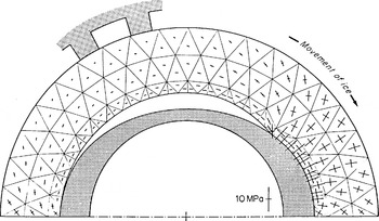
Fig. 10. Principal stresses at the element centroids (n = 3).
4.2. Relation between computation and experiment
4.2.1. Units and value of B in Glen’s flow law (3)
The length unit such as the dimensions of the finite-element mesh correspond to that of the apparatus is L = 1 m. The angular velocity O was measured very accurately thanks to the photographs and checked to remain constant for the duration of the experiment. It corresponded to a driving velocity U = 154.1 ± 0.5 m a−1. The resulting strain-rate unit is U/L = 154 a−1. The stress unit is derived from the comparison between the measured and computed values of the torque exerted by the ice on the torsion rod. The “theoretical” torque calculated from the Σn
distribution shown in Figure 6, with a sample thickness of 0.13L is C
th = 48.5 × 10⁻⁴
(σL3). The “experimental” torque is taken as the average  of the observed values (see Fig. 4), T being the period during which quasi-steady state was achieved. According to Reference Mellor and ColeMellor and Cole (1981), a better value C
e, accounting for the non-linearity of Glen’s flow law, would be such that
of the observed values (see Fig. 4), T being the period during which quasi-steady state was achieved. According to Reference Mellor and ColeMellor and Cole (1981), a better value C
e, accounting for the non-linearity of Glen’s flow law, would be such that

In the present case, the fluctuations of the torque, compared to C e or C exp, are small enough so that the two estimates are very close. The average value, taking into account a friction torque of 600 N m, is C exp = 4150 Nm The C exp/C th ratio gives the stress unit: σ = 0.85 Mpa (8.5 bar).
The resulting viscosity unit is σL/U = 1.74 ×10¹¹ Pa s (= 0.055 bar a), and the corresponding value of coefficient B in Glen’s flow law (3) is: B = U/(La3) = 7.92 × 10⁻²⁴ Pa-3 s-1 (= 0.25 bar-3 a-1). This value will be discussed later.
4.2.2. Shape of the cavity
Diagrams of the cavity profile have been made using the photogaphs taken at time t0 then after one and four revolutions of the machine (times t1 and t4 in Figure 4). Figure 11 shows the variations of ρ (measured to the millimetre) versus θ for the points on the cavity roof. A slight increase of the cavity volume can be noted between the extreme measurements. The computed cavity corresponds well to observations, especially for the one obtained after one revolution (t = t1 ).
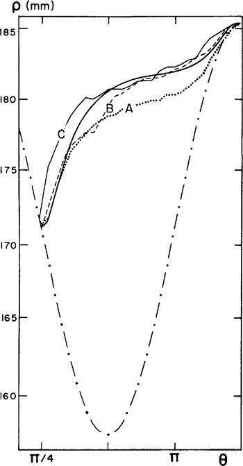
Fig. 11. Radius ρ(θ) of the cavity roof: (A) cavity observed at t = t0 (beginning of observations), (B) cavity observed at t = t1 (after one revolution), (C) cavity observed at t = t4 (after four revolutions). Solid line: cavity computed with n = 3; dotted line: polar radius of the bump profile.
4.2.3. Deformation of the marker network
The trajectories are solutions of the differential system:

Each trajectory is defined by its starting point M 0 on the radius θ = π. The solution to Equations (6) is found starting from M 0 at time t = 0 = t0 and using the Runge-Kutta method. At time t, the current point M belongs to element e. The position of M at t + Δt is calculated using the nodal velocities solution to finite-element system (5) and the interpolation functions specific to element e. The time step Δt is taken small enough so that, if M crossses the boundary of e during Δt, its new position can be kept. This computation was performed for 19 stream lines, equally spaced at 5 mm on the radius θ = п. Figure 12 shows the deformation of the material line θ = 0, initially radial, after one and four revolutions.

Fig. 12. Computed deformation (n = 3) of the radial line θ = 0: (0) initial position; (1) after one revolution; (4) after four revolutions (this line is not part of the network which is already deformed at time t0).
During the experiment, the ice trajectories are observed by following the displacement of each marker.
The comparison of the calculated and observed deformations of the network was made after one and four revolutions. The initial position of the network (instant t0 in Figure 4) is shown in Figure 13. In order to reduce the computational burden, each individual marker trajectory was linearly interpolated between the two nearest among the 19 already computed trajectories. The results are shown in Figures 14 and 15. After one revolution the computed and observed networks are practically the same. After four revolutions the results remain quite good: the mean deviation in the angular position θ of the markers is 1°.

Fig. 13. initial position of the marker network (time t0 in Figure 4).
4.2.4. Time description of the trajectories
More detailed checking of the flow can be carried out by studying how a marker moves along its trajectory with time. The study is restricted to the description of half a trajectory (0 > θ > π). About 50 photographs are available to measure the angular position θ(t) of a marker. The computed values are 12 times more numerous. The results for a marker on the innermost stream line are shown in Figure 16. As the differences between the observed and calculated θ are very slight after half a revolution, instead of θ(t) this figure shows the angular difference θ(t) to a point which would turn at the constant speed of rotation Ω of the machine, i.e. θ(t) = Ωt − θ(t). The comparison is made by taking the rejoining point on a bump as the starting point of the trajectory. It can be noted that when passing over the cavity, the differences θ are slightly greater for the marker than for the theoretical material point, which indicates a smaller increase in the observed
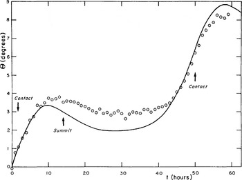
Fig. 16. Angular difference θ(t) = Ωt – θ(t) for a marker moving along the ice-bump contact and the cavity roof, o: observed; solid line: computed (n = 3) values.
velocity than that calculated with n = 3 in Glen’s flow law.
5. Discussion
5.1. Experimental conditions
Before discussing the results, it is necessary to look at how the assumptions used for the computation were handled during the experiment.
5.1.1. Steady-state conditions
The cold-room temperature is very difficult to maintain at a constant value over long periods. These temperature variations give rise to heat exchanges with the ice and are largely responsible for the torque variations (see Fig. 4).
On the other hand, the steady-flow assumption supposes that the shape of the cavities does not change. The measured increase in volume of a cavity between zero and four revolutions was about 100cm3, corresponding to a 1% decrease in the volume of ice, half of this variation taking place during the first revolution (volume of the cavity after four revolutions: 680 cm3). This decrease in the volume of ice was found to be mainly caused by melting at the bump contact, as heat was provided by the outer environment, further densification of the ice after time t = t 0 being undetectable (Reference MeyssonnierMeyssonnier, 1983). Two relatively important melting phases correspond to the decreases in torque recorded at times t = t 0 and t = t 2 in Figure 4.
Finally, it must be noted that the polar angle of the rejoining point varied little from the beginning to the end of the observations, passing from 44° to 43.5°.
5.1.2. Boundary conditions
The boundary conditions used for the computation and for which experimental validity must be verified are:
-
(a) frictionless ice-bump contact: in order to ensure the existence of a lubricating water film at the ice-bump interface, the melting temperature T m must be below the ambient temperature. According to Reference LliboutryLliboutry (1976): Tm = T0 − βpm − AN/w, where T0 is the melting temperature at normal atmospheric pressure, pm is the pressure at the ice-
water interface, β ≈ 0.1°C MPa−1 (Reference HarrisonHarrison, 1972), N is the number of saline equivalents per kg of ice, w is the water content, and A = 1.86°C kg mol−1. With p m = 6.5 Mpa, the mean normal stress corresponding to the measured torque, the drop in Tm is 0.65 C To reach the cold-room temperature N/w should be near 0.2 mol kg−1. This is quite a probable value as w was probably very low. During the experiment no disappearance of air bubbles was noticed which would have indicated melting at grain boundaries (Reference Barnes, Tabor and WalkerBarnes and others, 1971) and which was observed by Reference BrepsonBrepson (1979), who obtained a layer of blue ice totally free of bubbles when working at 0°C. Apart from the two short periods when melting was ascertained, ensuring perfect sliding, the friction should have remained very low at a temperature close to −1°C.
-
(b) driving condition: the adherence condition on the driving ring seems to be well represented if one refers to the deformation of the marker network after one and four revolutions (see Figs 14 and 15). A computation from a separate finite-element model (Reference MeyssonnierMeyssonnier, 1983) indicated that the sliding velocity over a driving cog, corresponding to a mean drag of 0.07 Mpa, is negligible (u b > 0.1 cm a−1). However, it can reach 2 m a−1 in zones where the tangential stress reaches its maximum value of 1 MPa (see Fig. 8).
-
(c) plane-flow hypothesis: the observations made on pieces of the ice sample collected at the end of the experiment did not show any appreciable inclination of the markers from the vertical.
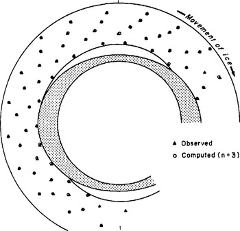
Fig. 14. Deformation of the marker network after one revolution (time t1 in Figure 4): о observed: Δ computed (n = 3).

Fig. 15. Deformation of the marker network after four revolutions (time t4 in Figure 4): о observed; Δ computed (n = 3).
5.2. Aptitude of the model for describing the observed behaviour
5.2.1. Value of exponent n in Glen’s flow law
The numerical results shown above were obtained with n= 3. This value is generally accepted for effective shear stress τ between 0.05 and 0.5 MPa (Reference Barnes, Tabor and WalkerBarnes and others, 1971; Reference DuvalDuval, 1976).
For higher values of τ, higher values of n have been reported in the literature (Reference SteinemannSteinemann, 1958; Reference Dillon and AnderslandDillon and Andersland, 1967; Reference Barnes, Tabor and WalkerBarnes and others, 1971). In general, values close to n = 5 have been quoted. Reference Goodman, Frost and AshbyGoodman and others (1981) explained these high values by the fact that at high stresses (τ > 1 MPa) the dislocation sliding velocity is no longer a linear function of stress. According to Reference Shöji and HigashiShôji and Higashi (1978) or Reference JonesJones (1982), creep at high stresses is accompanied by generalized micro-cracking, initiated by the piling up of dislocations at grain boundaries.
In the present model, τ = 1 MPa with n = 3 corresponds to a dimensionless value τ = 1.18(U/BL)1/3 or ![]() = 1.63(U/L). The extent of the region
= 1.63(U/L). The extent of the region ![]() > 1.5(U/L) covers all of the part situated up-stream of the bump (see Fig. 8). In order to take into account the results of the literature concerning high stresses, the computations were run again with values of n higher than 3.
> 1.5(U/L) covers all of the part situated up-stream of the bump (see Fig. 8). In order to take into account the results of the literature concerning high stresses, the computations were run again with values of n higher than 3.
First, n was taken equal to 4. The corresponding map of ![]() does not differ considerably from that obtained with n = 3. Therefore, the comparison is made primarily on the total deformations. Figure 17, which represents the computed deformation of the radial line θ = π/2 after four revolutions, shows that this deformation is of course more important when n = 4, but that the differences are only appreciable near the innermost stream line. For a point on this stream line, the angular difference between its positions computed with n = 3 and n = 4 after four revolutions is 5.6°. As for the deformation of the marker array, the difference in behaviour, already noticeable after one revolution, is very clear in the final position. The model with n = 3 already has a slight tendency to overestimate the deformations and this tendency becomes very pronounced with n = 4. This value must therefore be discarded.
does not differ considerably from that obtained with n = 3. Therefore, the comparison is made primarily on the total deformations. Figure 17, which represents the computed deformation of the radial line θ = π/2 after four revolutions, shows that this deformation is of course more important when n = 4, but that the differences are only appreciable near the innermost stream line. For a point on this stream line, the angular difference between its positions computed with n = 3 and n = 4 after four revolutions is 5.6°. As for the deformation of the marker array, the difference in behaviour, already noticeable after one revolution, is very clear in the final position. The model with n = 3 already has a slight tendency to overestimate the deformations and this tendency becomes very pronounced with n = 4. This value must therefore be discarded.

Fig. 17. Deformation of the radial line θ = π/2 after four revolutions, computed with n = 3 and n = 4.
In order to complete this work, the influence of a greater increase in n, but limited to the high effective shear-stress zones, was studied. To take such behaviour into account, Reference LliboutryLliboutry (1969) and Reference Colbeck and EvansColbeck and Evans (1973) have suggested adopting the polynomial relation ![]() = B
1
τ + B
3
τ
3 + B
5
τ
5, in which the linear term represents the behaviour at low stresses. In this work we preferred to use Glen’s flow law in which n is a (step) function of т. The viscosity is still given as n = B
−1
τ
1−n where n = 3 and B = B
3 for τ > τ
5; n = 5 and B = B
5 for τ
5 ≤ τ; the coefficients B
j being taken to preserve the continuity of the viscosity. In practice, the exact non-dimensional value of the threshold τ
5 which corresponds to a given stress cannot be fixed a priori (because the stress scale can only be fixed after calculation of the torque derived from the finite-element computation, and comparison to the measured one). Therefore, an approximate dimensionless value of τ
5 is chosen, based on the results obtained with n = 3, and it is verified a posteriori that the actual value of τ
5 corresponding to the experimental conditions is not too far from the desired threshold.
= B
1
τ + B
3
τ
3 + B
5
τ
5, in which the linear term represents the behaviour at low stresses. In this work we preferred to use Glen’s flow law in which n is a (step) function of т. The viscosity is still given as n = B
−1
τ
1−n where n = 3 and B = B
3 for τ > τ
5; n = 5 and B = B
5 for τ
5 ≤ τ; the coefficients B
j being taken to preserve the continuity of the viscosity. In practice, the exact non-dimensional value of the threshold τ
5 which corresponds to a given stress cannot be fixed a priori (because the stress scale can only be fixed after calculation of the torque derived from the finite-element computation, and comparison to the measured one). Therefore, an approximate dimensionless value of τ
5 is chosen, based on the results obtained with n = 3, and it is verified a posteriori that the actual value of τ
5 corresponding to the experimental conditions is not too far from the desired threshold.
The computation was made for a threshold τ
5 close to 1 MPa. The n = 5 region is then approximately limited by the contour ![]() = 1.5(U/L) in Figure 8. The ratio of the observed to the computed torques gives a pressure unit σ = 0.89 MPa and the corresponding actual threshold is τ
5 = 1.05 MPa. For a marker in contact with the bump, the angular difference with its position computed with и = 3 after four revolutions lies between 2.5° and 3°, depending on its initial position. The difference between the final deformations of the marker network is less pronounced than in the case n = 4.
= 1.5(U/L) in Figure 8. The ratio of the observed to the computed torques gives a pressure unit σ = 0.89 MPa and the corresponding actual threshold is τ
5 = 1.05 MPa. For a marker in contact with the bump, the angular difference with its position computed with и = 3 after four revolutions lies between 2.5° and 3°, depending on its initial position. The difference between the final deformations of the marker network is less pronounced than in the case n = 4.
5.2.2. Value of coefficient B in Glen’s flow law
The torque-measuring system is very accurate but part of the measured torque is due to the friction of the mobile upper plate on its inner fixed support. This friction torque depends very much on the tightening and lubrication of the sliding pad. It can only be estimated by destroying the ice sample, allowing the ice to melt on contact with the bumps (this is done by raising the cold-room temperature and letting the machine turn without dismantling the upper plate). This procedure was not adopted here, in order to preserve the sample. A friction torque of 600 N m, known to within 400 N m, was assumed. This corresponds to the average of values obtained in other tests at the end of which the ice was melted. The resulting uncertainty in the measurement of torque is 10%. It remains acceptable for the estimation of the stresses involved, but the accuracy of S, computed for n = 3, is only of the order of 30%.
In other experiments at the end of which friction was measured, B was found to lie between 6.34 × 10⁻²⁴ and 1.27 × 10⁻²³ Pa−3S-1 (0.2−0.4 bar-3 a-1).
The values of B computed with n different from 3 are:
(a) with n = 4: B = 7.6 × 10⁻³⁰Pa−4s−1 (0.024 bar−4a−1)
(b) with n = 3 if τ > τ 5, n = 5 if τ ≥ τ 5 = 1.05 Mpa;
B 3 = 7 × 10⁻²⁴Pa−3s−1 (= 0.22 bar−3a−1
B 5 = 6.3 × 10−36Pa−5s−1 (= 0.002 bar−5a−1
The values corresponding to n = 3 are higher than Reference DuvalDuval’s (1976), i.e. B = 3.17 × 10⁻²⁴Pa−3s−1 (= 0.1 bar−3a−1) at −0.05°C, for a low water content (w = 0.03%), and in a secondary creep state. This is due to the fact that at present deformation level tertiary creep is reached: re-crystallization and fabric formation contribute to increase the value of B. Comparison with Reference DuvalDuval’s (1981) value for tertiary creep and zero water content, B = 6.3 × 10⁻²⁴Pa−3 s−1 (= 0.2 bar−3a−1 indicates that w remained very low during our experiment.
5.2.3. Steady-creep hypothesis
During the experiment the ice is obviously not in a state of steady creep: stresses at a given material point are very different up-stream and down-stream of the bump (see Fig. 8).
Figures 18 and 19 show the mean angular differences θ (as defined in section 4.2.4) observed for the markers which travelled close to the ice-bump interface. These averages are calculated as follows:
-
(a) for each marker i, the observation allows θ at time tn = nΔt to be calculated
where Δt is the interval between. two photographs, Ω is the machine angular velocity, and θ
i
(tn
) is the polar angle of marker ; measured at time tn;
-
(b) a value of θ i (θm) for
is linearly interpolated through
-
(c) assuming that θ i (θ0) at θ0 = π (see Fig. 18) or θ0 = π/4 (see Fig. 19) for all the observed markers i, it is then possible to calculate an average ϴ(θ) corresponding to an Eulerian description of the flow.
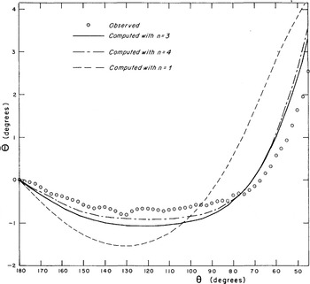
Fig. 18. Mean angular difference ϴ(θ) for the markers along the cavity roof, compared to those computed with n = 1, 3, or 4 (θ = 0 is assumed at the bump summit for each marker).

Fig. 19. Mean angular difference ϴ(θ) for the markers along the bump contact, compared to those computed with n = 1, 3, or 4 (θ = 0 is assumed at point θ = π/4 for each marker).
Figure 18 shows ϴ(θ) observed for markers which have passed the bump summit and are moving along the cavity roof. A comparison is made with the values calculated for ice obeying Glen’s flow law with n = 1, 3, or 4. Figure 19 gives ϴ(θ) for markers which have passed through the rejoining point and are travelling along the ice-bump interface.
First of all, it must be noted that a purely Newtonian model is not suitable for simulating the ice behaviour. Along the first three-quarters of the cavity roof, the points calculated with n = 3 or n = 4 are ahead of the observed average (see Fig. 18). This tendency is reversed when approaching the next bump. For a marker in contact with the bump, the accordance with the computation for n = 3 is excellent, except on approaching the bump summit (see Fig. 19).
The difference in behaviour observed between a theoretical Glen body and actual ice, down-stream of the bump, could be explained by the influence of transient creep occurring on unloading (Reference DuvalDuval, 1976; Reference Duval, Ashby and AndermanDuval and others, 1983). As for (re-)loading, no appreciable influence of Andrade creep (which appears upon loading of a virgin or annealed sample) can be noted. This result is in accordance with Reference LliboutryLliboutry’s (1975) estimations.
6. Conclusion
The analysis of the observed and computed final deformations of the marker array allows for the assumption of a Glen’s flow law exponent n higher than 3 to be discarded, and all the more so since the actual deformation is higher than or equal to that which would take place if the ice-bump contact were perfectly frictionless.
However, it remains possible that n could take a value higher than 3 for effective shear stresses τ greater than 1 MPa: the region involved would be too small for a
significant difference in behaviour to be detected by our method.
A more detailed study on how the observation markers move along their trajectories shows the difference in behaviour between ice and a purely viscous body, and the influence of transient creep. It appears that only transient creep on unloading may be significant.
The comparison betweeen the angular velocities θ deduced from the delay curves in Figures 18 and 19, and the computed values (shown in Figure 20), indicates that these transient effects can be ignored when the basal flow velocity of a glacier in steady-state conditions is to be simulated.

Fig. 20. Deviation from the constant speed of rotation Ω of the angular velocity ![]() of markers on the inner stream line: values of
of markers on the inner stream line: values of ![]() Comparison between computed values and those derived from the observed values of ϴ(θ)
Comparison between computed values and those derived from the observed values of ϴ(θ)
Acknowledgements
This study was carried out at the Laboratoire de Glaciologie et Géophysique de l’Environnement (C.N.R.S.-Grenoble, France), under the supervision of Professor L. Lliboutry, and with the financial aid of the Centre National de la Recherche Scientifique. Thanks are extended to Dr R. Brepson and Dr P. Duval, and to the late Professor P. Le Roy, for their helpful discussions and encouragement during the course of this work.


