1. Introduction

Glacial outburst floods released from proglacial, supraglacial, englacial or subglacial lakes can produce very high discharges, often with catastrophic consequences downstream (e.g. Reference Haeberli, Alean, Müller and FunkHaeberli and others, 1989; Reference Fountain and WalderFountain and Walder, 1998; Reference Richardson and ReynoldsRichardson and Reynolds, 2000; Reference RobertsRoberts, 2005; Reference Bajracharya and MoolBajracharya and Mool, 2009; Reference Dobhal, Gupta, Mehta and KhandelwalDobhal and others, 2013). Unlike proglacial and supraglacial lakes, englacial and subglacial water cavities cannot be detected easily (Reference LegchenkoLegchenko and others, 2011, Reference Legchenko2014; Reference Vincent, Descloitres, Garambois, Legchenko, Guyard and GilbertVincent and others, 2012). For this reason, they can represent a major invisible threat in densely populated mountainous areas. In Iceland, such reservoirs are filled by meltwater produced by subglacial volcanic warming (Reference BjörnssonBjörnsson, 1992, Reference Björnsson2003, Reference Björnsson2010; Reference Fountain and WalderFountain and Walder, 1998; Reference RobertsRoberts, 2005). Elsewhere, the processes leading to the formation and evolution of these intraglacial lakes remain unclear (Reference HaeberliHaeberli, 1983; Reference Walder and DriedgerWalder and Driedger, 1995).

Measurements from boreholes and dye injection experiments have helped us to better understand the subglacial water system (Reference Nienow, Sharp and WillisNienow and others, 1998; Reference Kavanaugh and ClarkeKavanaugh and Clarke, 2001; Reference Bingham, Nienow, Sharp and BoonBingham and others, 2005; Reference Sugiyama, Bauder, Huss, Riesen and FunkSugiyama and others, 2008). In addition, advanced models have been developed recently to simulate runoff changes in the subglacial water system of mountain glaciers (e.g. Reference Flowers and ClarkeFlowers and Clarke, 2002a,b; Reference Werder, Hewitt, Schoof and FlowersWerder and others, 2013). However, very few measurements are available on the evolution of intraglacial reservoirs. The main reasons for this are: (1) the rarity of such phenomena, (2) instrumentation problems encountered in subglacial environments (e.g. Reference ClarkeClarke, 2005) and (3) the fact that subglacial cavities are usually discovered only after they have triggered an outburst flood.

The deadliest outburst flood from an intraglacial cavity occurred on Glacier de Tête Rousse in the Mont Blanc area, French Alps, in 1892 and caused 175 fatalities (Reference Vincent, Garambois, Thibert, Lefèbvre, Le Meur and SixVincent and others, 2010). Reference Gilbert, Vincent, Wagnon, Thibert and RabatelGilbert and others (2012) showed that the thermal regime, mainly controlled by the snow cover thickness, and the geometry of the bedrock, are responsible for water storage inside this glacier, which is a polythermal glacier with negative temperatures in its lowest part (Reference Vincent, Garambois, Thibert, Lefèbvre, Le Meur and SixVincent and others, 2010; Reference Gilbert, Vincent, Wagnon, Thibert and RabatelGilbert and others, 2012). Periods with negative mass balances, associated with higher air temperature, tend to cool the glacier, whereas years with lower temperatures, associated with positive mass balances, tend to increase the glacier temperature by increasing the firn-pack depth and extent (Reference Gilbert, Vincent, Wagnon, Thibert and RabatelGilbert and others, 2012). In this way, the subglacial water is trapped by the cold lowest part of the glacier.

Between 2007 and 2010, new investigations were performed to check the potential existence of a subglacial water cavity in Glacier de Tête Rousse. Against all expectations, these studies revealed a subglacial lake (Reference Vincent, Descloitres, Garambois, Legchenko, Guyard and GilbertVincent and others, 2012; Reference LegchenkoLegchenko and others, 2014). The volume of water contained in the glacier was assessed at 53 500 m³, and data obtained from the boreholes and from surface nuclear magnetic resonance (SNMR) and ground-penetrating radar (GPR) measurements indicated that this water was contained in a single subglacial cavity. Reference Gilbert, Vincent, Wagnon, Thibert and RabatelGilbert and others (2012) showed from the measured and simulated temperature distribution in the glacier that this water had been enclosed for at least 30 years. In addition, the hydrostatic water pressure exceeded the ice pressure at the top of the cavity (Reference Vincent, Descloitres, Garambois, Legchenko, Guyard and GilbertVincent and others, 2012). Based on these geophysical and glaciological findings, public authorities were warned in July 2010 of the risk facing the 3000 inhabitants downstream of the glacier, and the subglacial reservoir was drained artificially by pumping in August 2010. Following this operation, the cavity refilled spontaneously during summer 2011 and was pumped again in September 2011. The same scenario occurred during summer 2012. Numerous measurements were performed to study the refilling of the cavity between 2011 and 2013.

The aim of this paper is to understand the behavior of the subglacial reservoir and the mechanisms that lead to the filling of the cavity. For these purposes, we analyze: (1) the water volume change almost continuously between 2010 and 2013 to infer the filling rate of the cavity following the pumping operations, (2) the changes of the cavity geometry during the periods of drainage and filling to study the mechanisms controlling these changes, (3) the origin of the water that fills the cavity, (4) the rate of the cavity refilling and (5) the velocity of surface melt transfer to the cavity. It is beyond the scope of this paper to model the hydromechanical processes that drive the water in the glacier. The main goal is to provide insight into the filling rates of the subglacial cavity, the water sources and the cavity response. We also discuss the possible drainage pathways leading to the subglacial cavity. The numerous observations conducted between 2010 and 2013 provide a great opportunity to analyze some of these mechanisms.

2. Data

2.3. Water-level measurements

In July 2010, 20 boreholes were drilled using hot water to determine the exact location of the cavity and monitor the ice temperature using thermistors (Reference Vincent, Descloitres, Garambois, Legchenko, Guyard and GilbertVincent and others, 2012). Four additional boreholes were drilled in July 2011 to reach the subglacial reservoir and survey its water level. The water levels were monitored in these boreholes using OTT Orpheus groundwater pressure sensors. Sensors No. 60, 61, 62, 63 and 64 were installed at depths of 74.6, 68.1, 52.8, 55.2 and 44.0 m below the surface respectively. The water level was recorded every 6 hours, starting with sensor No. 60 on 26 August 2010. This sensor broke down in February 2011. New sensors (Nos. 61–64) were set up in July 2011. After December 2011, sensor No. 61 broke down. A new borehole was drilled on 20 July 2012 to install a new sensor (No. 65) at 50.8 m depth. The water level was recorded every hour by this sensor. Sensor No. 64 stopped operating in October 2012. The sensor locations, altitudes and measurement periods are summarized in Table 1. Comparison between sensors reveals an accuracy better than 2 cm around the water level.

Table 1. Coordinates and measurement periods of water-level sensors

2.5. Meteorological measurements

At 3130 m a.s.l. and 90 m from the glacier (Fig. 1), a permanent automatic weather station (AWS) has been operating continuously since June 2010 (Table 2). The longwave radiation L terms were measured and corrected for sensor temperature. Therefore, the additional corrections recommended by Reference Obleitner and De WoldeObleitner and De Wolde (1999) were not used. Over the 2011 and 2012 ablation seasons, rainfall was measured using a heated tipping-bucket rain gauge at almost the same location (Fig. 1). To provide some help in detecting snowfall events, a time lapse camera produced six to seven frames per day of the main part of the glacier surface. A temporary weather station dedicated to surface energy-balance flux measurements stood freely on the glacier (Fig. 1) from the end of May to the end of October in 2011 and 2012 (Table 2). The sensors were mounted on a 2m high tripod. Tilt due to snow- and ice melt was limited by regularly readjusting the mast to vertical on the occasion of visits carried out every 10 days. At the same location, an acoustic ranger, mounted on steel stakes anchored in the ice, was used to measure the distance to the surface for snow depth and ice melt calculations.

Table 2. Meteorological measurements

Fig. 1. Map of the glacier surface. The cavity mapped in 2010 (black dotted line) is shown along with the locations of the boreholes in which sensors No. 60 to No. 65 were set up (blue dots). The meteorological stations are indicated by the two red triangles outside the glacier and the black triangle on the glacier. The hydraulic pathway calculated using the dye-tracer technique is shown by the blue dashed line. The surface mass balance was determined from measurements on the stakes shown in black. Horizontal and vertical ice flow was measured in the vicinity of the cavity using metal stakes shown in red. The red lines show the GPR measurements performed on two cross sections reported in Figure 4. The green line shows the sonar measurements carried out on a transverse cross section reported in Figure 5.

3. Subglacial Reservoir Evolution

The objective of this section is to analyze the filling of the cavity after the pumping operations of 2010, 2011 and 2012 in order to assess the filling rate of the cavity.

3.1. Water-level fluctuations in the subglacial cavity between 2010 and 2013

Water levels were continuously monitored in the boreholes between 1 July 2011 and October 2013 except when they were below the sensors. In addition, some measurements were available before and during the first pumping operation in 2010. The measurements are reported in Figure 2a. The large decreases observed after 2 July 2010, 28 September 2011 and 23 September 2012 are due to the artificial drainage operations using downhole pumps. The vertical positions of the sensors have an uncertainty of ±25 cm. However, the water-level changes measured by the different sensors are very consistent for water levels above 3155 m, with an uncertainty of 2 cm. The identical and simultaneous changes in water levels show that the connections between the boreholes have a very high hydraulic conductivity. Only sensor No. 63 shows a different evolution when the water level is <3155 m. Another discrepancy can be seen between sensors No. 62 and No. 65 for the period of 2013 during which the cavity refilled naturally. These discrepancies can be explained by the complex geometry of the lower part of the cavity, where the bedrock topography is likely rugged and includes several depressions (Reference Vincent, Descloitres, Garambois, Legchenko, Guyard and GilbertVincent and others, 2012). The filling rates and water levels in these depressions are independent until they are full and joined together. These boreholes are therefore temporarily unconnected or isolated from the glacier drainage system. Note that the slope of the refilling curve during summer 2011 is considerably less steep than that observed during the 2012 and 2013 summers. This indicates that the cavity geometry changes with time, very likely due to ice deformation and/or the fact that the refilling rate was not the same for both periods and depended on the available meltwater.

Fig. 2. (a) Water levels measured in the boreholes between 2010 and 2013. (b) Evolution of the volume of water within the cavity between 2009 and 2013 as determined by the volume of pumped water and modeled surface meltwater. The blue circles indicate volumes measured by the 3-D SNMR method (Reference LegchenkoLegchenko and others, 2014). The vertical dashed lines correspond to the beginning of successive pumping operations.

The subglacial cavity became full on 1 July 2012 and the water overflowed onto the ice surface. Between 1 July and 23 September 2012 (beginning of the pumping), we observed a slight decrease in the water level. During this period, a high ablation rate was observed, which lowered the surface altitude of the glacier. Consequently the slight decrease in the water level is explained by the altitude decrease of the boreholes through which the water overflowed. Moreover, due to the collapse of a snow/ice bridge in the cavity roof on 14 August 2012, a large crevasse full of water opened near the right side of the glacier (Fig. 1). The measured water-level changes show that this hole was an extension of the subglacial cavity, as also shown by GPR images. After this crevasse opened, the water in the cavity overflowed through this crevasse once the cavity was full.

A different pattern was observed during summer 2013 because winter accumulation was greater and ice remained under the snow cover (positive mass balance; Section 5.1 and Table 3). Consequently, surface ablation was lower. The large crevasse full of water in 2012 was not visible from the surface. As shown in Figure 2a, the water level was almost constant throughout this summer (Section 5.3).

Table 3. Mean and standard deviations of weather conditions, SEB terms and mass-balance terms from 25 May to 19 October 2011, 30 May to 23 October 2012 and 1 July to 31 October 2013

3.2. Water-volume changes using SNMR and pumping data

The link between the altitude of the water, which is well known from the pressure sensor measurements, and the total volume of water within the cavity is not straightforward. Moreover, due to the collapse of ice blocks from the cavity roof (detected by sonar and GPR measurements) and ice creep, the shape and total volume of the cavity is continuously evolving, altering the level-to-volume relationship. During the three artificial drainage operations, the extracted volumes of water, dv, were regularly measured together with the associated water-level variation dh. From these observations, we calculated the water volumes contained within the elevation ranges [h, h + dh] at which the measurements were performed. The refilling water coming from surface water supply was subtracted from dv. We also accounted for the permanent runoff that fills the cavity all year long (Section 5.2). Dividing the water volume by the elevation difference, we calculated the horizontal area of the cavity as a function of elevation A(h) = dv/dh (Fig. 3). In this way, we reconstructed the volume of the cavity as a function of elevation at these dates from

(1)

where the reference volume v _o at the level h _o is determined from the SNMR measurements, the total extracted volumes and the water-level measurements. For pumping in 2011 and 2012, the surface meltwater refilling the cavity during pumping was estimated from the surface energy model (Section 5.2) and used to correct the extracted volumes. For pumping in 2010, the refilling volumes are unknown due to the absence of the data required to estimate daily melting at the surface.

Fig. 3. The horizontal surface area of the cavity, A(h), as a function of the elevation as determined by the 2010 (black), 2011 (blue) and 2012 (red) pumping data.

Figure 3 shows that over the 3 years, the cavity presents a complex geometry and the horizontal sections vary greatly over the cavity depth. Clearly, the associated water-level–volume relationship (Eqn (1)) is highly nonlinear. Figure 3 also clearly reveals that the total volume of the cavity decreased over these 3 years of pumping. This is especially visible in the bottom part of the cavity, below 3130 m.

Artificial drainage could not extract all the water from the cavity, so the pumped volume of water underestimates the total volume of the cavity. Nevertheless, using the 3-D SNMR measurements before pumping (Reference LegchenkoLegchenko and others, 2014), the total volume is estimated and a residual volume after pumping is deduced. In this way and assuming a linear change of the cavity volume with time, the evolution of the volume of water within the cavity can be inferred from water-level changes. Figure 2b shows the evolution of the volume of water within the cavity from August 2010 up to the beginning of 2013. All the 3D-SNMR measurements performed over these 3 years are reported in Figure 2b. The cavity became full of water in each of the three summers and, since 2011, surface overflow has been observed from the holes drilled the previous years. This indicates that the total volume of the cavity strongly decreased from year to year, mainly as a result of the pumping and the creep of ice induced by an empty cavity as shown in Section 4.

4. Cavity Geometry Changes

The objective of this section is to study the cavity geometry changes in response to the drainage/filling of the cavity following the pumping carried out in 2010, 2011 and 2012 and to analyze the causes of these changes. The SNMR measurements clearly reveal a strong decrease of water volume between 2010 and 2012 (Fig. 2b). The cavity volume available for the water decreased over this period. The changes of the cavity geometry were thoroughly analyzed from GPR measurements, sonar, DEMs using GPS measurements performed on 20 September 2007 and laser-scan measurements performed on 10 August 2011, and surface horizontal and vertical ice flow velocities determined from theodolite measurements.

The radar measurements carried out in May 2010 and May 2011 on the same cross sections in the vicinity of the cavity, before and after the first pumping of August/September 2010, show strong changes within the internal structure of the glacier. An example is shown in Figure 4, where GPR transverse data, the locations of which are shown in Figure 1, were migrated using a velocity of 0.168 m ns⁻¹ and corrected for topography (Reference Vincent, Descloitres, Garambois, Legchenko, Guyard and GilbertVincent and others, 2012).

From the migrated radar images, we detected the cavity roof (Fig. 4). Depth 0 corresponds to an altitude of 3189 m for images on the left and to an altitude of 3192 m for those on the right. A generalization of the cavity roof depth picking to all available transverse and longitudinal GPR profiles surrounding the cavity was used to obtain the topography of the roof in May 2010, May 2011 and August 2011. Changes in this topography show that the thickness of the cavity roof strongly decreased. This decrease is obvious between May 2010 and May 2011, after the first pumping, and amounted to >20 m at some locations during this period. Given that the surface ablation was 0.86 m w.e. between 1 July 2010 and 1 May 2011, these observations reveal that the roof partially collapsed after the cavity was pumped. In addition, the sonar measurements performed in 2010 and 2011 show strong changes in the geometry. Although it was not possible to survey the entire cavity from the sonar instrument due to hidden faces and even though the measurements were performed from one borehole only, they show clearly that the bottom of the cavity was filled with ice. This very likely came from the collapse of the roof when the cavity was empty, with the ice blocks freezing to the bottom. Indeed, after the pumping performed at the end of the summer and during the winter, the cavity was almost free of water. Water can freeze easily in this area where the bedrock is near or below the freezing point (Reference Gilbert, Vincent, Wagnon, Thibert and RabatelGilbert and others, 2012). An example of sonar measurements is given in Figure 5. These reveal that the bottom of the cavity rose by 13–30 m. This is also confirmed by the change in the horizontal area of the cavity as a function of the elevation between 2011 and 2012 (Fig. 3), obtained from extracted water volumes during pumping operations. These observations provide evidence that the bottom of the cavity rose by ∼30 m. However, from radar and sonar measurements, it is very difficult to assess the shrinking of the cavity because radar measurements can only detect the roof, and sonar measurements concern a part of the cavity only.

Fig. 4. Evolution of the two transverse profiles shown in Figure 1 between May 2010 and August 2011. Cross sections (a), (c) and (e) are located downstream of cross sections (b), (d) and (f).

The volume change of the cavity can also be estimated using (1) SNMR measurements and (2) surface displacement measurements. Ice being incompressible and the horizontal flow negligible on this glacier (<0.8 m a⁻¹), the volume loss by glacier surface subsidence is equal to the volume lost by the cavity through creep, corrected for the mean ablation/ accumulation over the study period. Consequently, if no other process occurs, it should be similar to the volume loss obtained from SNMR measurements over the same period for a water-filled cavity.

Fig. 5. Cross section of the glacier with the surface (blue) and bedrock (gray). The geometry of the cavity obtained from sonar measurements carried out on 1 September 2010 and 23 September 2011 is plotted in black and red solid lines respectively. The dashed lines correspond to the roof of the cavity obtained from GPR measurements in May 2010. The vertical blue line is the borehole from which the sonar measurements were performed.

First, the volume change calculated using the SNMR method was assessed at 30 000 m³ between August 2010 and September 2011. For these two dates, the cavity was full of water, although it was pumped in September and October 2010 and refilled during spring and summer 2011. No SNMR measurements were carried out in August 2010, but we can assume that the volume in August 2010 was similar to that in September 2009, given that the cavity was continuously full of water during this period.

Second, the surface subsidence from August 2010 to August 2011 was estimated from two digital elevation models (DEMs) obtained on 20 September 2007 and 10 August 2011 (Fig. 6). Given that the cavity was full of water between September 2007 and August 2010, we assume a negligible vertical flow during this period. The September 2007 DEM was corrected by −3.20 ±0.30 m to account for the ice ablation between 20 September 2007 and 10 August 2011, determined by numerous ablation measurements using the ablation stakes. Finally, the difference between this corrected DEM and the 10 August 2011 DEM provides the vertical displacements between August 2010 and August 2011.

Fig. 6. Vertical displacements from August 2010 to August 2011 derived from DEMs obtained in 2007 and 2011. The DEM difference was corrected for the ice ablation measured over this period. The black solid line shows the location of the cavern obtained from sonar measurements.

From this method, the volume lost by the cavity by creep is evaluated to be 14 300 ± 5000 m³, with a maximal vertical surface displacement of 2.80 ± 0.30 m in 1 year. The loss by creep can therefore explain 48 ± 17% of the volume change measured by the SNMR method. The remaining volume loss could be explained by the porosity of the collapsed ice at the bottom of the cavity. Indeed, this ice coming from the roof of the cavity is made of blocks. The collapse occurred when the cavity was empty. Given that this ice remains at the bottom of the cavity following the filling, one can assume that these ice blocks were frozen to the bedrock. The initial high porosity of the ice-blocks layer offered a much larger interface for thermal exchange, certainly allowing refreezing of a large quantity of water during the winter filling. Another part of the volume loss might be explained by a partial closure of the cavity following the pumping and the strong creep deep below the surface. In this way, part of the cavity was possibly isolated and would therefore not fill with water.

These observations show that the changes in cavity geometry following the pumping operations were due both to ice creep and the internal collapse of the cavity roof. In particular, the collapse of the roof led to the opening of a crevasse in August 2012 on the right side of the glacier where the roof was thin.

To assess the ice creep before and after pumping, we measured the vertical displacements from a surface network of 30 stakes located in the vicinity of the cavity (Fig. 1) during summer 2011. The displacements were measured using a total station between 25 May and 17 November 2011 with a time interval of a few days to 4 weeks (Fig. 7). The objective was to assess the rate of expansion and closure during the filling and pumping phases. These observations clearly reveal a subsidence when the cavity was partially empty, with vertical displacements of up to −4 mm d⁻¹ in the vicinity of the cavity center. Conversely, when the cavity is almost full and the water level reaches 3150 m, 20 m below the surface, we observed an uplift with velocities of up to +4 mm d⁻¹. In Figure 7, we report the average vertical displacement obtained from the whole stake network. We compared the vertical displacement with the water level and concluded that the buoyancy level was 3150 m. Figure 7 shows the comparison with the vertical displacements measured in 2010 (Reference Gagliardini, Gillet-Chaulet, Durand, Vincent and DuvalGagliardini and others, 2011). It reveals large differences in subsidence displacement rates when the cavity is empty. These differences can be explained by the size of the cavity which was much smaller in 2011. When the water level exceeded 3132 m, the behavior was very similar. From these observations, we conclude that the vertical velocity is a very good indicator of filling as soon as the water level reaches the cavity roof.

Fig. 7. Mean vertical ice flow velocities measured in the vicinity of the cavity after pumping and during the refilling. In 2011 the bottom of the cavity was filled with ice coming from the roof collapse, which explains the different behavior below 3130 m and a similar behavior above. Date format is dd/mm/yy.

5. Feeding of the Subglacial Reservoir

Two crucial questions concern the origin of the water that fills the cavity and the cavity-filling rate. To address these questions, we studied the relationship between surface melting and filling.

5.1. Daily surface melting from energy balance

Surface meltwater was estimated in 2011 and 2012 from a surface energy-balance (SEB) calculation. Calculations were coupled with the ultrasonic ranger measurements to optimize some parameters of the SEB. A simple temperature-index method was also used for comparison in 2011 and 2012, and used on its own in 2013 to provide surface melt without recourse to SEB. The melt factors were determined from ablation stake measurements to preserve the independence of both approaches and provide an independent control.

The energy balance at the glacier surface dictates that radiative and sensible heat balance latent heat fluxes associated with mass exchanges due to change of state. The SEB that represents the heat content in a unit mass available for melt is written as (Reference OkeOke, 1987)

(2)

where S↓ is the global radiation (shortwave irradiance), S↑ is the reflected shortwave radiation, L↓ and L↑ are the longwave irradiance and emittance, H is the turbulent flux of sensible heat and LE the turbulent latent heat due to sublimation. R is the sensible heat associated with rainfall (liquid precipitation). F is the energy provided by meltwater flowing at the glacier surface from conversion of gravitational potential energy into heat. This term was neglected in the balance. Q _w is the energy sink required to balance the sensible heat stored by the winter thermal cold wave near the glacier surface. Given that it is found on the right-hand side of Eqn (2), the latent energy term related to fusion Q _f is conventionally defined as positive.

Under clear-sky conditions, the systematic error in shortwave radiation measurements due to the slope of snow and ice surfaces (15° towards the east) was applied using the formulation of Reference Grenfell, Warren and MullenGrenfell and others (1994) as soon as the global radiation exceeded 70% of the extraterrestrial irradiance corrected for shading. From the end of May to the end of October, this reduced the shortwave irradiance by 12% on average over 2011 and 2012.

The Q _w flux was fixed at −1 W m⁻² from the temperature gradient of −0.25°C m⁻¹ measured between the glacier surface and 12 m depth (Reference Gilbert, Vincent, Wagnon, Thibert and RabatelGilbert and others, 2012). The sensible heat flux R was calculated with precipitation rates provided by the rain gauge assuming the rain to be at air temperature. Turbulent fluxes were calculated using the bulk aerodynamic approach. We included stability corrections (Reference Price and DunnePrice and Dunne, 1976) as the surface layer was found to be predominantly under damped forced (stable) conditions as inferred from calculations of the Richardson number. For the choice of the roughness length, we found the best match between ablation calculated from the SEB and ablation measured with the ultrasonic ranger using z ₀ = 0.1 cm. Ablation measured at stake 4 in the vicinity of the weather station located on the glacier was used as an independent check on the ablation provided by the SEB. We found a reasonable agreement, the discrepancy being <0.1 m w.e. over the ablation duration periods of 10–20 days over which stakes were routinely measured. Air temperature, solid and liquid precipitation, daily energy fluxes, albedo and the resultant SEB are plotted in Figure 8 for the 2011 ablation season. Mean recorded values for the 3 years of the study are given in Table 3.

Fig. 8. Daily energy fluxes from 25 May to 20 October 2011. (a) Potential extraterrestrial (top-of-atmosphere) shortwave irradiance (dashed line) and the same variable corrected for shading by surrounding mountains (dotted line); measured global radiation (S↓) and air temperature (T). (b) Incoming longwave radiation (L↓), net shortwave radiation (S), turbulent fluxes of sensible (H) and latent (LE) heat and surface energy balance (SEB). (c) Liquid and solid precipitation and albedo.

5.2. Surface meltwater and filling of the subglacial cavity

Using the energy-balance calculations, the cumulative surface melt was reconstructed for the years 2011–13 . The cumulative melt and rainfall were compared in detail to the water volume changes obtained from water levels, pumping and SNMR data during summer 2011 (Fig. 9). The cumulative melt and rainfall cannot be converted to water volume given that the drainage surface area is unknown. However, from these data, it is possible to infer: (1) the delay between surface melting/rain and the observed filling water in the cavity and (2) the surface area of the drainage basin needed to fill the cavity.

Fig. 9. Water volume in 2011 as reconstructed from water level, pumping and SNMR data (blue line), and cumulative melt given by the SEB (dashed line), including rainfall (red line). Bars are daily melt on a mm scale. The slope of 14 m³ d⁻¹ reveals the daily filling runoff observed between 18 and 31 July without surface melting.

For this purpose, we first calculated the cross-correlation between surface melting/rain and the filling water using different time lags (Fig. 10a). The analysis was done with a time interval of 1 day given that the water level was recorded every 6 hours between July 2011 and July 2012. The water levels recorded every hour at sensor No. 65, available after July 2012 only, are analyzed in Section 5.3. The obtained cross-correlation curve is rather flat. This is due to the intrinsic autocorrelation of the daily meteorological signal that governs melting. The significance threshold of correlation is given by the dashed line in Figure 10a. From this analysis, the best correlation (0.64) is obtained with a delay of 1 day. The analysis performed in Section 5.3 provides more accurate results from hourly records.

Fig. 10. Relation between melt and filling daily rates in 2011 (excluding rainfall days). (a) Cross-correlation between melt rate and deferred cavity-filling rate as a function of the time lag; the dashed line is the significance threshold. (b) Linear correlation between filling rate and melting at day +1 for the days without precipitation. The intercept is the filling rate expected without melting. The sensitivity is equivalent to an effective draining surface area of 3000 m².

Although these results provide only a rough approximation of the time lag between melting and filling, they do show that the time lag does not exceed 4 days. Using these results, we calculated the regression coefficients between daily melting and the filling rate at day +1. The correlation was calculated for periods without precipitation. We obtained a sensitivity of 30 m³ cm⁻¹ w.e. The surface area of the drainage basin that feeds the cavity is therefore 3000 m². This is small compared to the glacier-covered surface area located upstream of the cavity, which is 30000 m². In addition, the regression curve of Figure 10b shows a residual intercept identifying a permanent filling rate of 33 m³ d⁻¹ when melting is zero. This suggests that the cavity is fed by permanent internal runoff, not depending on surface melting and associated meteorological surface conditions.

This permanent runoff is confirmed by a thorough analysis over the following periods. During summer 2011, there was a cold, dry period between 18 and 31 July 2011. Although the energy-balance calculations and ablation and precipitation measurements revealed the absence of melting and rain, the cavity-filling rate was assessed at 14 m³ d⁻¹ for 14 days. Moreover, analyses of filling rates during the 2010/11 and 2011/12 winters lead to the same conclusions. After the end of pumping in October 2010, the cavity was refilled during winter 2010/11 and spring 2011. From SNMR measurements performed on 5 June 2011, we calculated that the filling volume was 4760 m³ between October 2010 and June 2011. From meteorological data, the water volume coming from surface melting was estimated at 1030 m³ over this period. This indicates a permanent runoff of 16 m³ d⁻¹ during the winter and spring that is not related to any surface meltwater. The same analysis carried out on the period between 9 October 2011, after pumping, and 8 June 2012, corresponding to the SNMR measurements, led to a filling volume of 6160 m³. Taking into account the water volume from surface melting, i.e. 2170 m³, the filling rate from permanent runoff was assessed at 15 m³ d⁻¹, which is in good agreement with the previous estimates.

We then investigated the role of the geothermal heat flux as a potential source for the winter runoff. Applying a geothermal heat flux of 20 mW m⁻² (Reference Gilbert, Vincent, Wagnon, Thibert and RabatelGilbert and others, 2012) to the surface of the upstream watershed that is covered by snow in winter (surface area 55800 m²), we found a runoff of 0.32 m³ d⁻¹ coming from basal melting. In any case, the runoff from the basal melting cannot exceed 1m³d⁻¹, even when considering the total surface area of the drainage basin covered by snow during the winter and doubling the geothermal heat flux.

We therefore suspect that this permanent runoff is caused by another water reservoir located upstream within the glacier. The permanent filling rate identified in the ablation season is slightly higher than that identified over the winter months. This discrepancy is not necessarily contradictory considering: (1) error due to the scattering of the regression curve of Figure 10b and (2) a possible seasonality dependence due to the available meltwater in summer.

5.3. Transfer velocity of meltwater between the surface and the cavity

To estimate the time required for the water to be transferred from the surface to the cavity, we used two methods.

First, dye-tracer experiments were carried out in the bergschrund (Fig. 1) on 28 September 2012 during pumping. In this way, the dye tracers were detected by a fluorometer set up at the exit of the pipe used for pumping. Considering the detection threshold (presence/no-presence) of 1 ppb, the Rhodamine arrived at the fluorometer 5 hours after the injection (Fig. 11). The dye concentration increased between +5 and +24 hours after the injection, reaching a maximum value of 14.5 ppb. Twenty-four hours after the injection, the Rhodamine concentration decreased abruptly to 0.4 ppb. Considering the pumped water volume and the Rhodamine concentration time series, the mass restitution is only 4 g, which represents 1% of the injected tracer. The pumped water temperature was 1°C during the experiment. In response to the salt injection, the conductivity shows a slight increase from 60.1 to 74.7 μS cm⁻¹ between the beginning and end of the experiment.

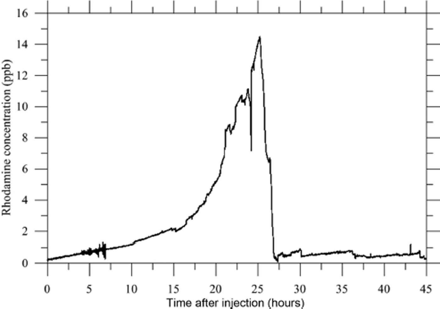
Fig. 11. Dye tracing with 30 s time-step data since 28 September 2012 at 11:00 LT. The dye was injected at 12:00 LT. The dye concentration in the pumping water at the fluorometer is expressed in ppb and the detection threshold is 1 ppb.

The conductivity increase is due to the natural stratification existing in the cavity with denser (salty) water at the bottom. From this experiment, we can conclude that: (1) a hydraulic connection exists between the injection point and the cavity, separated by a straight line distance of at least 243 m, (2) the liquid water velocity is at least 50 m h⁻¹ (0.014 m s⁻¹) (a lower limit considering that the hydraulic pathway may be longer but not shorter) and (3) only a small portion of the Rhodamine was resituated (1%) and the increase in concentration stopped abruptly 24 hours after the injection.

The second method used to calculate the transfer velocity was based on a thorough analysis of the time delay between the occurrence of surface melting and rain and the water-level changes inside the subglacial reservoir (Fig. 12). The time delay was calculated from the water-level measurements using sensor No. 65, which provides hourly records starting on 20 July 2012. We used half-hourly runs of the SEB model to provide hourly averages of surface meltwater. We calculated the cross-correlation between surface melting/rain and the water-level changes using different time lags. To conduct this analysis, we took advantage of a period (2–11 September 2012) of well-contrasted day/night melting/refreezing conditions providing acute midday melt signals (Fig. 12), making it possible to detect a time lag with acceptable accuracy. The best correlation was obtained with a time delay of 4–5 hours on average and ranging from 2 to 10 hours.

Fig. 12. Relationship between water level of the cavity, melt and rainfall from 24 August to 10 October 2012. The cross-correlation between melt rate and deferred cavity-filling rate as a function of the time lag is reported in the inset. The dashed line is the significance threshold.

This relatively high dispersion of the time lag is reasonable as meltwater was produced for 9–12 hours according to the SEB model, so water injection into the glacier cannot be considered instantaneous.

To confirm and improve the estimated time delay between surface melting and the filling of the cavity, we also analyzed a period during which a huge liquid precipitation event occurred on 29 July 2013 (Fig. 13). At the beginning of the period, between 25 and 26 July, diurnal melting was observed but no night melting. We observed oscillations of both melting and water level, with a time delay of 5–7 hours. The water level at piezometer No. 65 was stable on a daily average basis. During the night of 26–27 July, high temperatures and strong wind caused a high sensible heat flux, and night melting began at 03:00. Melting occurred continuously throughout the day on 27 July. It was also observed during the night of 27–28 July. The water-level oscillations can be clearly identified between 26 and 28 July. On a daily average basis, the water level recorded at piezometer No. 65 increased from 27 to 28 July due to the supply of meltwater during the night. On 29 July, from 02:00 to 22:00, a severe thunderstorm produced 49 mm of rain over 20 hours. Between 02:00 and 06:00, the instantaneous rain intensity reached 40 mm h⁻¹. Moreover, in addition to the rainfall, the air temperature of 4°C caused night melting and supplied further water. The huge liquid precipitation of 29 July provided a depth of water three to four times higher than the water depth usually provided by melting (1.2 cm w.e. h⁻¹ vs 0.3–0.4 cm w.e. h⁻¹). This event can be seen as a natural injection of water over the whole surface area of the glacier. The water level at piezometer No. 65 reached a maximum of 3169.67 m at 10:00. From these observations, we found that the water level increased with a time delay of ∼6 hours after the rain reached its maximum intensity. This result, although less accurate than a precisely located and instantaneous artificial water injection, is consistent with the time delay obtained by the dye-tracing experiments and the previous cross-correlation calculations.

Fig. 13. Changes in water level recorded at piezometer No. 65, melt and rainfall from 25 July to 2 August 2013. Date format is dd/mm/yy.

6. Discussion

The important question concerning the supply of the cavity, especially during the winter when no melting occurs, remains unsolved. In September 2013, another intraglacial reservoir was found in the upper part of the glacier (Reference LegchenkoLegchenko and others, 2014) in the vicinity of large crevasses located between 3220 and 3230 m a.s.l. (Fig. 1). The volume of the upper reservoir is assessed at 18500 ± 5500 m³. The radar measurements carried out in 2014 in the upper part of the glacier show that this upper reservoir could very likely be a water-filled crevasse. No direct field measurements could confirm this conclusion, given that the glacier has been covered by snow in this area over the last 2 years. Radar images show a large crevasse extending 50–60 m deep in the glacier (Fig. 14). Given that ice flow is low, this crevasse is very likely water-filled. Moreover, between this upper reservoir and the main subglacial cavity downstream, the radar images show a 15–20 m thick basal ice layer with a large amount of spread energy (scattering, reflectors), which was used to delineate the cold–temperate transition surface (Reference Pettersson, Jansson and HolmlundPettersson and others, 2003). These reflections are caused by scattering from small water voids present in the temperate ice beneath the cold surface layer. The temperature measurements performed in the drillholes in this region (Reference Vincent, Descloitres, Garambois, Legchenko, Guyard and GilbertVincent and others, 2012) confirm that this 15–20 m thick layer is temperate, with cold ice above. This suggests that the upper reservoir is connected to the main subglacial cavity through this temperate ice layer and/or through a permeable layer of rock debris at the glacier bed. This could explain the permanent runoff of 14–20 m³ d⁻¹ throughout the year. However, it does not explain how the water coming from melting or rain, with large runoff, is conveyed from the surface to the main subglacial cavity. From our observations, we attempted to characterize the subglacial pathways that carry the surface meltwater and rain to the central subglacial reservoir. From the comparison of surface melting/rain and filling, and from dye-tracer experiments, we found a time lag of 4–6 hours between the water input from the surface and the filling of the cavity. Note that the same time lag was obtained with high and low runoff. A major question concerns the route and the type of channels through which the water is conveyed.

Fig. 14. Longitudinal cross section of the glacier from GPR measurements.

To deal with this question, we determined the route of the water coming from the dye-tracer injection location using the water pressure potential. For this calculation, the water pressure is assumed equal to the pressure of the overlying ice. In this way, the water pressure potential Φ can be calculated using (Reference PatersonPaterson, 1994)

(3)

where z _s is the altitude of the glacier surface, z is the bedrock altitude,ρ_i is the density of ice,ρ_w is the density of water and g is the gravitational acceleration. Using the surface and bedrock DEMs, it is possible to calculate the path of the water from the entry point of the dye tracer. The route is perpendicular to the hydraulic equipotentials and follows the highest hydraulic gradient. The length of this hydraulic pathway from the surface to the bedrock is then L = 294 m (i.e. 17% longer than the rough straight line pathway used in Section 5.3). Given that the hydraulic potential difference expressed in m of water is ΔΦ = 92.5 m along this track, the hydraulic gradient is ΔΦ/L = 0.315. We consider again the 2–11 September 2012 period for which surface runoff rate of transfer to the cavity was quantified. We estimated the discharge for the period 2–11 September 2012, for which the surface melting was 1.14 cm d⁻¹ over an average time of 10.5 hours each day. Using the previously obtained drainage surface area of 3000 m² (see Section 5.2), the volume of water is estimated at 34.2 m³ over 10.5 hours each day. This gives an average discharge of q = 9.048 × 10⁻⁴ m³ s⁻¹ from the surface to the subglacial reservoir. With the time delay of 4–6 hours identified in Section 5.3 by the cross-correlation between surface melting and water-level change, we calculated a water flow velocity of 0.017 ± 0.003 m s⁻¹ along the 294 m of the hydraulic pathway. This is in good agreement with the dye-tracer results (0.014 m s⁻¹) obtained 18 days later. From the discharge and the average transfer velocity, the average cross-sectional area of an intraglacial channel between the surface and the subglacial reservoir is assessed at s = 0.0532 m². Assuming an equivalent circular conduit, this corresponds to an average radius of 13 cm. Assuming the validity of Darcy’s law and assuming a drainage effective porosity equal to 1, the ‘Darcy’ permeability K inferred from the water flow velocity, the average cross section and the hydraulic gradient is given by

(4)

This leads to K = 0.054 m s⁻¹, which is a typical permeability of rather open-permeable subglacial sediments (Reference FlowersFlowers, 2000).

From this analysis, we conclude that the water coming from the upper part is not drained by a tunnel system or a channelized system. Indeed, the mean flow velocities in channelized drainage systems are of the order of 0.3–1 m s⁻¹ (Reference Nienow, Sharp and WillisNienow and others, 1998; Reference Cuffey and PatersonCuffey and Paterson, 2010). Here we found a value of 0.017 m s⁻¹, which is characteristic of a rather slow drainage system. It is comparable to flow velocities between 0.012 and 0.068 m s⁻¹ obtained by Reference NienowNienow (1993) for a distributed drainage system, or 0.03 m s⁻¹ at Midtdalsbreen, Norway (Reference Willis, Sharp and RichardsWillis and others, 1990). The flow velocities we found in our study are similar to those obtained in a linked-cavity system, with a network of many interconnected cavities. However, cavities are generally reported to form under rapid sliding conditions (Reference NyeNye, 1970; Reference WalderWalder, 1986; Reference KambKamb, 1987; Reference Fountain and WalderFountain and Walder, 1998). Here the ice surface velocities are very low, <0.4 m a⁻¹ in this region, and sliding, if any, would not be able to open cavities. Consequently, the drainage of Glacier de Tête Rousse is likely not a linked-cavity system. Alternatively, the drainage could occur in a macro-porous horizon of permeable layers at the top of the sediment (porous subglacial sheet as described by Reference Flowers and ClarkeFlowers and Clarke, 2002a). Glacier de Tête Rousse is likely underlain by a continuous layer of rock debris which may act as an aquifer. This assumption is supported by the value of hydraulic conductivity. Hydraulic conductivity values inferred from in situ measurements in glaciological studies vary greatly. From borehole measurements carried out on South Cascade Glacier, Washington, USA, Reference FountainFountain (1994) estimated the hydraulic conductivity range from 10⁻⁷ to 10⁻⁴ m s⁻¹. Using similar methods, Reference Iken, Fabri and FunkIken and others (1996) found a hydraulic conductivity of 0.02 m s⁻¹, a value typical of coarse gravel. The review of Reference Fountain and WalderFountain and Walder (1998) shows considerable variability in the hydraulic conductivity from in situ estimates, ranging from 10⁻⁷ to 10⁻² m s⁻¹. Sediment studies performed in the Trapridge Glacier (Canada) forefield reveal hydraulic conductivities of 10⁻⁵−10⁻³ m s⁻¹ (Reference StoneStone, 1993). Reference Flowers and ClarkeFlowers and Clarke (2002b) adopted hydraulic conductivity values of subglacial sediment ranging between 2.5 ×10⁻² and 5.0 ×10⁻² m s⁻¹. The hydraulic conductivity calculated from flow velocities and the hydraulic gradient at Glacier de Tête Rousse is roughly consistent with these values. Consequently, it is likely that the subglacial water flows through a permeable layer of rock debris at the glacier bed.

We therefore suspect that the drainage of the water coming from the upper reservoir occurs through this layer or along the interface between the ice and its substrate. As suggested previously, it is probable that a large part of the drainage occurs along beds of sediment. The upper reservoir would then be responsible for the permanent runoff during the winter when no meltwater or rain comes from the surface. In this way, the upper reservoir, constituted by the water-filled crevasse, supplies water throughout the year with similar hydraulic conductivities and an almost constant hydraulic head. During the summer, the water from melting and rain follows other pathways from bergschrunds or crevasses to reach the bedrock and fill the main subglacial cavity.

6. Conclusions

Our study provides insight into the filling of the subglacial cavity of Glacier de Tête Rousse and into the drainage pathways leading to the subglacial reservoir. This cavity was drained artificially in 2010, 2011 and 2012. From our observations, we reconstructed the water volume changes and the filling rates of the subglacial reservoir continuously between 2010 and 2013. We found a strong relationship between the observed surface melting and the filling rate with a time delay of 4–6 hours. The amount of available surface meltwater upstream of the cavity is 10–15 times greater than the quantity of water that fills the reservoir. The surface area of the drainage basin that feeds the cavity is ∼3000 m². It is small compared to the glaciated surface area located upstream of the cavity.

Depending on the weather conditions and the size of the cavity, the subglacial cavity can be filled with a typical runoff of 76 m³ d⁻¹, i.e. within 4–5 months for a 10000 m³ cavity. In addition, our analysis reveals a permanent runoff that supplies the cavity independently of surface melting and rain. This permanent runoff is in the range 14–20 m³ d⁻¹ and appears to be relatively constant whatever the season when no surface melting or rain occurs.

From dye-tracing experiments, we found a time delay of 4–5 hours between the bergschrund and the subglacial cavity, consistent with the time delay obtained from the comparison between melting or rainfall inputs and water-level changes. The intraglacial reservoir found in the upper part of the glacier is likely the cause of the permanent runoff feeding the main subglacial cavity. Radar images strongly suggest that this upper reservoir is a water-filled crevasse extending 50–60 m deep, i.e. close to bedrock.

This water-filled crevasse does not explain the large runoff that supplies the cavity during intense melting or rain events. The meltwater and rain from the surface is conveyed to the bedrock through other crevasses or through the bergschrund. Once the bedrock is reached, the water follows a drainage pathway between the upper reservoir and the central subglacial cavity. It seems this pathway is located in the basal layer of the glacier given that we found a temperate 15–20 m thick layer at the base of the glacier under the cold ice. Given the flow velocities and the inferred hydraulic conductivity, it is probable that the subglacial water flows through a permeable layer of rock debris at the glacier bed. When the water reaches the subglacial cavity, it is trapped by the cold and impermeable lower part of the glacier (Reference Vincent, Descloitres, Garambois, Legchenko, Guyard and GilbertVincent and others, 2012). Here the subglacial water of Glacier de Tête Rousse cannot escape through the ice/bed interface of subsurface aquifers. The filling rate supplying the main subglacial cavity ranged from 15 m³ d⁻¹ during the winter to 130 m³ d⁻¹ on average during summer 2011. Thus, when melting or rain occurs, the runoff into the cavity largely exceeds the permanent runoff of 15 m³ d⁻¹.

Our study also provides insight into the geometry changes of the main cavity with time, depending on water filling and the water pressure inside the cavity. From SNMR water volume measurements, we found that the cavity volume strongly decreased after each pumping operation. Creep explains a large part of the volume loss. The ice creep was assessed from the subsidence of the surface after pumping in 2010. It explains about half of the cavity volume changes. Moreover, from radar and sonar measurements, there is some evidence that the cavity roof partially collapsed following pumping and the decrease of the water pressure. Thus, the remaining volume loss could be explained by the porosity of the collapsed ice at the bottom of the cavity. Another part of the volume loss could come from the partial closure of the cavity due to ice creep which could have left part of the cavity unfilled.

The vertical displacements of the glacier surface observed from stakes located in the vicinity of the cavity clearly reveal ice subsidence when the cavity is empty and uplift when the water level reaches 3150 m, i.e. 20 m below the surface. From these observations, we assessed the rates of expansion and closure during the filling and pumping phases. The subsidence velocity can reach −12 mm d⁻¹ in the vicinity of the cavity center. When the cavity is almost full, the uplift reaches +4 mm d⁻¹, leading to an increase of the cavity volume. These observations show that the vertical velocity measurements are a very good indicator of the filling as soon the water level reaches the cavity roof.

In July 2013, the cavity was once again full of water and it was decided, given the estimated volume of water inside the cavity, not to renew the artificial drainage of the cavity (still true in autumn 2014). In comparison to the situation in 2010 with a pressurized cavity, the water level in the cavity is now limited at maximum to the surface elevation due to the numerous holes drilled from the surface during the three drainage operations and also to the break-off of part of the cavity roof on 14 August 2012. Due to the difference in hydrostatic pressure, the rate of decrease in the volume of an empty cavity is approximately nine times faster than the rate of increase in volume when the water level is equal to the upper surface elevation.

Finally, this analysis provides insight into the thermal or mechanical processes that could explain the formation of the subglacial cavity. Temperature measurements carried out in previous studies (Reference Vincent, Descloitres, Garambois, Legchenko, Guyard and GilbertVincent and others, 2012) showed a polythermal structure, explaining why subglacial water was trapped by the cold and impermeable lowest part of the glacier (−2°C) (Reference Gilbert, Vincent, Wagnon, Thibert and RabatelGilbert and others, 2012). Moreover, temperature measurements and modeling suggest that this subglacial water reservoir has existed for at least 30 years. Indeed, Reference Gilbert, Vincent, Wagnon, Thibert and RabatelGilbert and others (2012) showed that the cavity may have started to grow between 1970 and 1980. The thermal mechanisms that could influence the geometry of the cavity are inefficient. Heat transfers capable of melting the cavity roof are very low given that the water temperature is close to zero (Reference Vincent, Descloitres, Garambois, Legchenko, Guyard and GilbertVincent and others, 2012). Conversely, energy transfers through the roof and sides of the cavity are not sufficient to refreeze the stored water (Reference Gilbert, Vincent, Wagnon, Thibert and RabatelGilbert and others, 2012). The only efficient mechanism involves hydraulically driven fracturing and ice deformation around a high water pressure zone (Reference Van der VeenVan der Veen, 1998, Reference Van der Veen2007). High water pressure, exceeding the ice-overburden pressure as measured in 2010 when the subglacial cavity was discovered from boreholes (Reference Vincent, Descloitres, Garambois, Legchenko, Guyard and GilbertVincent and others, 2012), is sufficient to lift the glacier and form a subglacial cavity. Although this mechanism depends on the geometry of the cavity, our measurements show that the uplift velocity can reach several mm d⁻¹. The subglacial cavity was ∼30 m high when it was discovered in 2010. Assuming that it has existed for 30 years (Reference Gilbert, Vincent, Wagnon, Thibert and RabatelGilbert and others, 2012), the mean uplift velocity would be 3 mm d⁻¹ over this period, although it was probably not constant.

Author Contribution Statement

C. Vincent wrote most of the paper, coordinated the work and the various analyses. He was assisted by the co-authors. More specifically, E. Thibert collected and analyzed data on surface energy and mass balance and their incidence on the water level of the cavity. O. Gagliardini reconstructed the water volumes held in the cavity from SNMR and artificial drainage data and analyzed the cavity geometrical changes from sonar, radar and DEM data. S. Garambois collected and analyzed GPR data. A. Gilbert and T. Condom carried out the dye-tracing experiment and its analysis. A. Legchenko, J.M. Baltassat and J.F. Girard performed and analyzed the SNMR measurements.