


1. INTRODUCTION
Subglacial water flow has long been the subject of glaciological studies (see Clarke, Reference Clarke1987, for a historical overview). Early quantitative treatments of subglacial drainage were motivated by a diverse range of problems: Weertman (Reference Weertman1962) considered how a water layer at the glacier base impacts sliding, Röthlisberger (Reference Röthlisberger1972) developed his theory of channelised flow (through R channels) in connection with hydro-power generation related work, and Nye (Reference Nye1976) extended R channel theory with time-dependence to investigate glacial lake outburst floods. Recent developments in subglacial drainage theory have been driven largely by the motivation to better understand, represent and model glacier sliding, outburst floods and subglacial sediment dynamics in models.
It is indeed this link to ice dynamics that spurred the most recent, ongoing burst of subglacial drainage model development. As of yet, we do not fully understand the impact on ice dynamics of increased surface melt in a warming climate (e.g. Vaughan and others, Reference Vaughan2013). For glaciers and land-terminating portions of the ice sheets, an acceleration in ice flow may lead to increasingly negative mass balance by moving ice to lower, warmer, elevations (Ridley and others, Reference Ridley, Gregory, Huybrechts and Lowe2010). In temperate glaciers, a large fraction of mean ice velocity is due to slip of the glacier over its bed (e.g. Engelhardt and Kamb, Reference Engelhardt and Kamb1998; Cuffey and Paterson, Reference Cuffey and Paterson2010; Morlighem and others, Reference Morlighem, Seroussi, Larour and Rignot2013). This basal slip is a combination of both sliding of the glacier ice over its bed and deformation of any water saturated till layer underlying the ice (Cuffey and Paterson, Reference Cuffey and Paterson2010). Both components of slip are primarily driven by the presence of water at the base of the glacier, in particular, by its pressure (e.g. Iken and Bindschadler, Reference Iken and Bindschadler1986; Iken and others, Reference Iken, Echelmeyer, Harrison and Funk1993; van de Wal and others, Reference van de2008). Therefore, to assess the impact of increased surface melt on ice dynamics, we need to determine the response of the subglacial system to enhanced water input; current theories and models suggest that water pressure and hence ice flow speed, could either increase or decrease, depending on the nature of the subglacial drainage (e.g. Shannon and others, Reference Shannon2013; Sole and others, Reference Sole2013; Doyle and others, Reference Doyle2014; Tedstone and others, Reference Tedstone2015; Joughin and others, Reference Joughin, Smith and Howat2018).
The scarcity of data and the complexity of the subglacial system makes it difficult to pinpoint the water-induced processes acting at the base of glaciers. Thus, numerous theoretical models have been developed since the 1960s to mimic the flow of water at the beds of the glaciers (e.g. Weertman, Reference Weertman1962; Röthlisberger, Reference Röthlisberger1972; Nye, Reference Nye1973; Walder, Reference Walder1986; Kamb, Reference Kamb1987; Creyts and Schoof, Reference Creyts and Schoof2009). These theoretical models have been motivated by specific needs, preferences and practical considerations, leading to a plethora of models. The different approaches used make it difficult to compare the diverse theories that they implement. For example, over the last couple of decades, a number of subglacial hydrology models have been developed that compute basal water pressure directly from meltwater input (e.g. Flowers and others, Reference Flowers, Bjornsson, Palsson and Clarke2004; Werder and others, Reference Werder, Hewitt, Schoof and Flowers2013; de Fleurian and others, Reference de Fleurian2014) and a comprehensive overview is given in Flowers (Reference Flowers2015).
This intercomparison project sets out to alleviate the problem of multiple theoretical approaches to subglacial hydrology by establishing a set of synthetic simulation suites and comparing the results of the participating models running those simulations. This should help potential model users make a more informed decision as to which model to choose for a specific application. Likewise, for model developers, this may assist in assessing where further model developments are needed and provide a set of reference models against which to compare future ones.
The aim of this intercomparison is different from that of ice-sheet model intercomparison projects (Huybrechts and others, Reference Huybrechts and Payne1996; Payne and others, Reference Payne2000; Pattyn and others, Reference Pattyn2008, Reference Pattyn2012, Reference Pattyn2013). In the latter case, the physics of ice flow are reasonably well established, although boundary conditions remain less clear and are usually specified as parts of the setup.
For subglacial hydrology, however, a complete and ‘true’ theory is lacking. In other cases, such as the ice-thickness estimation intercomparison ITMIX (Farinotti and others, Reference Farinotti2017), a set of measurements is available which allows the assessment of the most appropriate model to apply. Unfortunately, observations of subglacial drainage are sparse, difficult to interpret (e.g. borehole measurements Rada and Schoof, Reference Rada and Schoof2018) and unlikely to fully constrain all the parameters of a subglacial drainage model (e.g. Brinkerhoff and others, Reference Brinkerhoff, Meyer, Bueler, Truffer and Bartholomaus2016). Furthermore, to date, applications of subglacial drainage models to real topographies and forcings are few and often hampered by modelling difficulties. Recognising these limitations and following the line of preceding intercomparison exercises, we opted for synthetic test cases which were better able to detect differences in physical or numerical approaches through qualitative comparisons.
Note that this intercomparison does not attempt to verify or validate the results provided by the participating models. Instead, SHMIP aims to provide a set of benchmark experiments tailored to compare existing and future subglacial hydrologic model in spite of their varied implementations. This intercomparison will also indicate which models will likely be appropriate for certain applications in subglacial hydrology. All results of this SHMIP exercise are openly accessibly at de Fleurian and others (Reference de Fleurian2018).
We first give a brief overview of subglacial drainage modelling and describe the physics implemented by the participating models. We then describe the approach taken by SHMIP and the different suites of experiments, before presenting results from the 13 models. Finally, we provide a synthesis of model results, and discuss strengths and potential shortcomings based on these results.
2. THE WIDE VARIETY OF SUBGLACIAL HYDROLOGY MODELS
By design, this intercomparison exercise allowed participation of any model that calculates effective pressure (defined as ice overburden pressure minus subglacial water pressure). The project thus attracted a wide range of models: from a zero-dimensional (0-D) lumped element model to models simulating the entire two-dimensional (2-D) glacier bed. Models ranged from ones developed in the 1980s to others under current development and from models simulating one component of the system, for instance R channels, to models coupling several components. Table 1 gives an overview of the participating models.
Table 1. Summary of the participating models

The model label is defined as the two initials of the experimenter; if the used model was published/written by someone else, then one initial of the original author is appended (e.g. cdf); models implemented by the experimenter from a published model are cited as ‘from: original publication’; two different models of the same experimenter are distinguished by a subscript number; two submissions of the same model using different parameters are distinguished by a prime. ‘Suites’ lists the Suites for which model results were submitted. ‘Dim.’ gives the number of spatial dimensions of the model, which is used in the text to differentiate between them, that is 0-D, 1-D or 2-D models. ‘Model Type’ is a brief description of the type of model, which is used throughout the text; these are defined within the section ‘Subglacial hydrology modelling’. ‘Parameters different from Table 3’ shows which parameters have been changed from the base-case Run, please refer to the supplementary for parameters of the models requiring tuning. ‘PDMP’ states if the model introduces a pressure dependence to the melting point.
The components of the drainage system are commonly classified into two types: inefficient (slow) drainage and efficient (fast) drainage, with the former usually represented as a distributed system and the latter as a channelised system (e.g. Flowers, Reference Flowers2015). This difference is a consequence of how the steady state of each system transforms under increasing discharge: in an inefficient system pressure increases, because steeper pressure gradients are required to conduct the increased discharge; conversely, in an efficient system pressure decreases, as the system's capacity increases sufficiently to allow operation at lower gradients.
In many of the participating models, the inefficient component of the drainage system is based, at least partially, on a linked cavity drainage system using, either discrete elements (Kessler and Anderson, Reference Kessler and Anderson2004) or a 2-D sheet (Hewitt, Reference Hewitt2011). The efficient component, if it is included, is usually represented by Röthlisberger channels (R channels) following Röthlisberger (Reference Röthlisberger1972). The cdf model uses a different type of water sheet (or inefficient system) based on Flowers and others (Reference Flowers, Bjornsson, Palsson and Clarke2004). Two models (bf and sb) pursue a different strategy modelling the drainage as a porous aquifer in order to approximate discharge through both the inefficient and efficient system. In the following section, the different types of drainage systems are briefly described. For a more in-depth comparison of subglacial drainage models, refer to the excellent review paper by Flowers (Reference Flowers2015).
2.1. Subglacial hydrology modelling
Common to all participating models is the use of a conservation of water equation, which takes the form:
 $$ \displaystyle{{\partial h} \over {\partial t}} + \nabla \cdot {\bf q} = m,$$
where h is the local size of the water body (height, area or volume, depending on the formulation), q is the water flux and m is a source term (accounting for meltwater input from the surface via the englacial system as well as water produced by geothermal flux, by frictional heat from sliding and by heat produced by dissipation in the subglacial flow). The second common ingredient is the use of a ‘water flow law’ relating q with hydraulic potential gradient  $\nabla \phi $ using a linear (Darcy flow) or nonlinear relation (Darcy--Weisbach or Manning)
 $${\bf q} \propto \nabla \phi \quad {\rm or}\quad {\bf q} \propto \sqrt {\nabla \phi },$$
where the hydraulic potential ϕ = p w + ρ w gz is the sum of water pressure p w and elevation potential (with water density ρ w, acceleration due to gravity g and elevation z). The factor of proportionality may depend on other state variables, in particular, h. Both these equations can be applied in 2-D (a sheet), in 1-D (a channel or width integrated water sheet), or in 0-D (integrated over the whole domain).
However, these are only two equations for three unknowns q, ϕ and h, so a third equation is needed to close the mathematical description of the subglacial drainage system. Typically, this equation describes the size of the drainage space. The different participating models implement this third equation in various ways, discussed in the following subsections. Furthermore, some models couple two drainage types together.
2.2. Sheet drainage
Over the years several formulations of water draining through a distributed system, often called a sheet drainage system, have been proposed (e.g. Weertman, Reference Weertman1962; Walder, Reference Walder1986; Kamb, Reference Kamb1987; Creyts and Schoof, Reference Creyts and Schoof2009). The participating models use two types of sheet-like drainage. The first, proposed by Flowers and Clarke (Reference Flowers and Clarke2002), is an empirical relation between water sheet thickness h and water pressure p w based on data from Trapridge Glacier (Canada)
 $$p_w = p_i\left( {\displaystyle{h \over {h_c}}} \right)^{7/2},$$
where p i is ice overburden pressure and h c is a critical sheet thickness. A model implementing this type of sheet drainage system will be referred to as a macroporous-sheet model (Table 1).
The second formulation used by some of the participating models is based on a linked cavity drainage system (Walder, Reference Walder1986; Kamb, Reference Kamb1987). In a 1-D setting, this formulation was advanced by Kessler and Anderson (Reference Kessler and Anderson2004) and Schoof (Reference Schoof2010). Hewitt (Reference Hewitt2011) then generalised it to 2-D by using a cavity height averaged over a suitably large patch of the glacier bed. The formula takes the form of a rate equation for h (cavity cross-sectional area in 0-D and 1-D or average sheet height in 1-D and 2-D) that, when saturation is assumed, reads:
 $$\displaystyle{{\partial h} \over {\partial t}} = v_o - v_c,$$
where v o is an opening rate, typically dependent on the sliding rate and bed roughness, and v c is a closure rate due to ice creep. One possible form is
 $$v_o = h_ru_b\quad {\rm and}\quad v_c = \displaystyle{{2A} \over {n^n}}hN^n,$$
where h r is the bed roughness height, u b is the ice sliding speed, A is the ice rate factor, n is Glen's exponent and N = p i − p w is the effective pressure. A model implementing this type of sheet drainage system will be referred to as a cavity-sheet model (Table 1).
Note that in most models the opening term, v o, does not contain the energy dissipation term (c.f. next section) which was in the original description (Walder, Reference Walder1986; Kamb, Reference Kamb1987), as its implementation is not trivial (Dow and others, Reference Dow, Karlsson and Werder2018) and it can lead to mathematical issues such as runaway growth of drainage space (Schoof and others, Reference Schoof, Hewitt and Werder2012). As an exception, model as does include opening by melt from dissipation, in conjunction with a different approach to the momentum equation (2) (Sommers and others, Reference Sommers, Rajaram and Morlighem2018). For a more detailed overview of sheet-like drainage consult the excellent overview given in Bueler and van Pelt (Reference Bueler and van Pelt2015).
2.3. Channelised drainage
The classic theory of channelised subglacial drainage, through R channels, was developed by Röthlisberger (Reference Röthlisberger1972) and Shreve (Reference Shreve1972). Further work extended the theory to include time dependence and also water temperature as a free variable (Nye, Reference Nye1976; Spring and Hutter, Reference Spring and Hutter1982) and to enable the use of broad low conduits, rather than semi-circular ones (Hooke and others, Reference Hooke, Laumann and Kohler1990). Whereas other theories of channelised drainage exist, such as canals (Walder and Fowler, Reference Walder and Fowler1994) (although these can also be considered as a type of distributed system), all of the participating models implementing channelised drainage use R channels. Furthermore, none of the participating models include water temperature as a state variable and instead assume that water temperature is always either at the pressure melting point or at 0°C. The equation describing the channel cross-sectional area S is similar to the cavity-sheet equation
 $$\displaystyle{{\partial S} \over {\partial t}} = V_o - V_c.$$
The closure V c is again by ice creep and is identical to Eqn (5) (replacing h by S). Conversely, channel opening is due to ice melt at the channel walls
 $$V_o = \displaystyle{{ - Q{\mkern 1mu} {\phi }^{\prime} + c_tc_w\rho _w{\mkern 1mu} Q{\mkern 1mu} p^{\prime}_{{w}} \over {\rho _iL}},$$
where the prime′ is short for the spatial derivative  $\displaystyle{\partial \over {\partial s}}$ along the channel, c t is the Clapeyron slope, c w the heat capacity of water, ρ i the density of ice and L the latent heat of fusion. The first term in the numerator is the energy dissipation in the flow (i.e. mechanical energy converted to thermal energy by the flow). The second term takes into account the changes in sensible heat due to pressure melting point variations, with the Röthlisberger constant c t c w ρ w ≈ 0.3. This second term can be neglected if the water is assumed to be always at 0°C. A model implementing this type of R channel drainage will be referred to as a one-channel model, if it involves only one channel, or a channels model, if it involves a network of channels (Table 1).
The equations of a single cavity Eqn (4) and an R channel Eqn (6) can be combined into one
 $$\displaystyle{{\partial S} \over {\partial t}} = v_o + V_o - V_c$$
(Kessler and Anderson, Reference Kessler and Anderson2004), sometimes termed a conduit (Schoof, Reference Schoof2010), thus giving a drainage element that opens both by sliding and by melting. When opening by sliding dominates, the system behaves like a cavity; otherwise it is like an R channel. A model implementing this type of drainage system will be referred to as a conduit model (Table 1).
Equations (1), (2) and (6) describe a single R channel. However, the subglacial system is thought to consist of a network of these channels. Relatively recent advances (Schoof, Reference Schoof2010; Hewitt, Reference Hewitt2013; Werder and others, Reference Werder, Hewitt, Schoof and Flowers2013) have made the simulation of such a network of R channels possible.
2.4. Porous layer drainage
The approach to modelling a network of R channels described above has several drawbacks, such as having to resolve each channel with the mesh and having no obvious continuum limit. This, among other things, inspired the development of porous layer drainage models. Such models do not try to simulate the drainage system as described by the theory presented above but instead use one or several porous layers as being equivalent to different types of subglacial drainage. Porous layers are usually considered an inefficient drainage system (Shoemaker, Reference Shoemaker1986), but with proper parameter choice these layers can be configured to be as transmissive as highly efficient systems (Teutsch and Sauter, Reference Teutsch and Sauter1991). These models also rely on mass-conservation Eqn (1) and Darcy flow Eqn (2). To close the model, either a fixed layer thickness h is assumed, or the layer evolves as a function of the pressure.
Two main approaches are used to simulate systems with different efficiencies within this porous layer framework. In the first, several layers with different conductivities are used. In the second, a single layer is used and the conductivity (the constant of proportionality in Eqn (2)) is allowed to evolve. The porous layer models included here assume a non-zero compressibility (βl), which adds a significant amount of storage S s:
 $$S_s = \rho _wg\omega h\beta_l $$
where ω is the porosity of the layer. A model implementing this type of drainage system will be referred to as a porous-layer model (Table 1).
2.5. Additional drainage elements
Additional drainage elements, such as drainage through till (e.g. Flowers and Clarke, Reference Flowers and Clarke2002) are incorporated in some subglacial drainage models. In the participating models, the only additional process included is the variation of water storage as a function of water pressure. The storage in the englacial system is considered to be well connected to the subglacial system (i.e. the englacial water table height corresponds to the subglacial water head). This necessitates a modification of the conservation equation (1)
 $$\displaystyle{{\partial h} \over {\partial t}} + \displaystyle{{\partial h_e} \over {\partial t}} + \nabla \cdot {\bf q} = m,$$
to include the thickness of the effective storage component h e, which is given in terms of the water pressure h e = e vp w/ρ wg in which e v is the englacial void fraction.
2.6. Coupling of components
Subglacial drainage is thought to occur through different types of drainage systems, co-evolving in space and time and exchanging water (e.g. Iken and Truffer, Reference Iken and Truffer1997). To approximate this complex behaviour, many models couple multiple system components together. One example is the conduit mentioned above Eqn (8), combining an R channel and a cavity. Table 1 gives an overview over the coupled systems of each model. Additional details on each model are given in the supplementary materials. A model implementing several types of drainage systems will be referred to as the combination of systems it implements forexample cavity-sheet/channels model and macroporous-sheet/one-channel model (Table 1).
3. INTERCOMPARISON DESIGN AND SETUP
The present intercomparison project deviates from many previous ones involving other components of the ice dynamic system, as there is no established theory of subglacial drainage, nor are there any sufficiently dense datasets that would allow reasonably conclusive comparisons with reality. This scenario prevents both validation and verification of the models participating in the intercomparison (Oreskes and others, Reference Oreskes, Shrader-Frechette and Belitz1994). With these limitations in mind, we designed the intercomparison around six synthetic Suites of experiments (labelled from A to F) each consisting of a set of four to six numerical experiments, subsequently referred to as Runs. The setup and detailed instructions are available onlineFootnote 1 and the website contents are included in the supplementary material. The Suites are designed to allow a wide variety of models to take part in the intercomparison and to test a large range of scenarios. This design allowed the participation of 13 models that completed some or all of the experiments. The main requirement was that models should output the effective pressure, which is used as the main diagnostic variable throughout the intercomparison. This approach excludes models based on a routing-approach (e.g. Le Brocq and others, Reference Le Brocq, Payne, Siegert and Alley2009) and the till-layer based models (e.g. Bougamont and others, Reference Bougamont2014). These alternative models do not explicitly compute effective pressures but instead use a pressure field unrelated to the state of the drainage system.
3.1. Topographies
The intercomparison uses two different synthetic glacier topographies (Fig. 1). The first (Fig. 1a), used for Suites A to D is a synthetic representation of a land-terminating ice sheet margin as seen, for instance, in Werder and others (Reference Werder, Hewitt, Schoof and Flowers2013). The ice-sheet domain is 100 km long (in the x direction) and 20 km wide (in the y direction), with a flat bed, parabolic ice surface and a maximum ice thickness of 1500 m:
 $$\matrix{ {z_s(x,y)} \,\,{ = 6{\mkern 1mu} (\sqrt {x + 5000} - \sqrt {5000} ) + 1,} \hfill \cr {z_b(x,y)} \,{= 0,} \hfill \cr } $$
where z s and z b are the surface and bed elevation in metres, and x and y are the horizontal spatial coordinates in metres. To avoid numerical issues, the minimum ice thickness is 1 m.
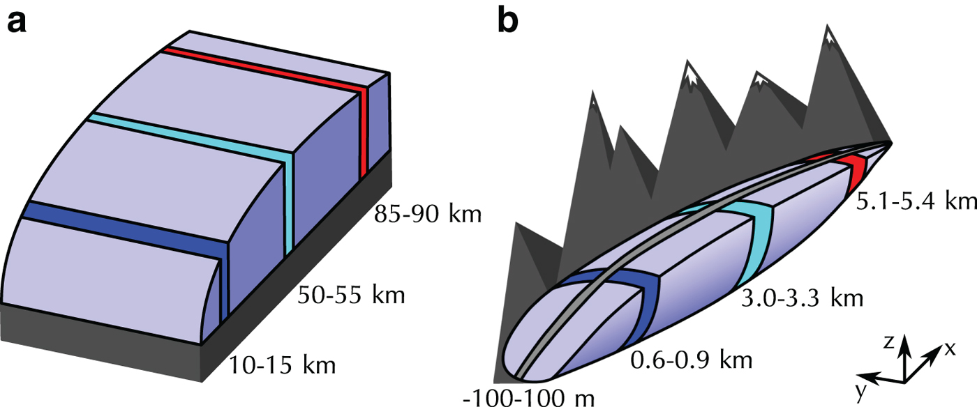
Fig. 1. Sketches of the topographies used, (a) 100 km long synthetic ice-sheet margin with a maximum thickness of 1500 m, and (b) 6 km long synthetic valley glacier with a 600 m altitude difference between summit and terminus. The coloured and gray bands are the regions used in presentation of the results.
The second topography (Fig. 1b), used for the Suites E and F, is a synthetic valley-glacier geometry inspired by Bench Glacier, AK, USA (e.g. Fudge and others, Reference Fudge, Humphrey, Harper and Pfeffer2008). The glacier is 6 km long and 1 km wide, with a difference in altitude between the terminus and the head of 600 m. Its shape is given by the following two equations:
 $$\matrix{ {z_s(x,y)} \hfill \,{ = 100{\mkern 1mu} \root 4 \of {x + 200} + \displaystyle{x \over {60}} - \root 4 \of {2 \times {10}^{10}} + 1,} \hfill \cr {z_b(x,y,\gamma )}\,{ = f\,(x,\gamma ) + g(y){\mkern 1mu} {\mkern 1mu} h(x,\gamma ),} \hfill \cr } $$
in which γ is a parameter controlling the bed overdeepening, and f, g and h are helper functions defined as follows:
 $$\matrix{ {\,f\,(x,\gamma )}\,{ = \displaystyle{{z_s(6000,0) - 6000{\mkern 1mu} \gamma } \over {{6000}^2}}x^2 + \gamma {\mkern 1mu} x,} \hfill \cr \quad {g(y)}\,{ = 0.5 \times {10}^{ - 6}{\mkern 1mu} {\mkern 1mu} {\rm \vert}\,y\vert^3,} \hfill \cr {h(x,\gamma )}\,{ = \displaystyle{{\left( { - 4.5{\mkern 1mu} x/6000 + 5} \right){\mkern 1mu} (z_s(x,0) - f\,(x,\gamma ))} \over {z_s(x,0) - f\,(x,\gamma _b) + {10}^{ - 16}}},} \hfill \cr } $$
where γ b = 0.05 is the parameter that is used as a reference γ and which gives the closest matching bed elevation to that of Bench Glacier. By design, the glacier boundary is the same for all γ and its half-width is given by
 $$y_o(x) = g^{ - 1}\left( {\displaystyle{{z_b(x,0) - f\,(x,\gamma _b)} \over {h(x,\gamma _b) + {10}^{ - 16}}}} \right).$$
3.2. Boundary conditions
For the two geometries, the boundary conditions are prescribed to give a realistic distribution of water pressure. The most important boundary is the margin of the ice sheet (x = 0 km) or terminus of the glacier (x = y = 0 km) where the water pressure is required to be null. The flux at this boundary is then free to evolve. All the other boundaries are treated as zero-flux boundaries.
3.3. Parameters and optional tuning
The two topographies are complemented by a set of physical parameters (see Table 3), which are used in the cavity-sheet/channels drainage formulations Eqns (1)–(10). Experimenters using models that implement this cavity-sheet/channels formulation (or a very similar one) were instructed to use the provided parameters in their model Runs. Note that the englacial void fraction e v is different for Suites A–D and Suites E–F.
However, a wider range of physics is incorporated in the participating subglacial hydrology models (and presumably future models that may use this intercomparison as a test setup), and this requires additional and/or different parameters. This further hampers an intercomparison of models based on different physics. To circumvent this difficulty, models whose parameters are not captured in Table 3 are tuned to the width-averaged effective pressure output of two reference Runs of a model employing the cavity-sheet/channels formulation (GlaDS model, mw, tuning instructionsFootnote 2). Optionally, modellers could also tune using the provided width-averaged sheet and channel discharge. The chosen reference Runs are two steady-state Runs with low and high recharge (Runs 3 and 5 from Suite A, Fig. 2m) that correspond to a sheet-only state and to a channelised state of model mw, respectively. The models that used tuning are cdf (only A5), jd (only A5, for high discharge), as (only A3), sb and bf (a red label in Fig. 2 indicates a tuned model, with the white outline showing the tuned Runs). Most tuned models only used the provided effective pressure but model as which was also roughly tuned to discharge. Note that the tuning was optional and that lack of tuning would not preclude participation. However, no model with parameters diverging from that of the reference model were submitted without tuning. Nevertheless, the prescribed tuning is unlikely to constrain all parameters of a subglacial drainage model, for instance any parameters reflecting transient behaviour will not be constrained. However, we feel that this tuning strategy presents a balance between making the model outputs comparable without requiring models employing other physics to over-fit and thus pushing them into a regime that is not representative for them. Finally, results that are different from the reference Run do not mean that the corresponding model is less correct, but merely different.
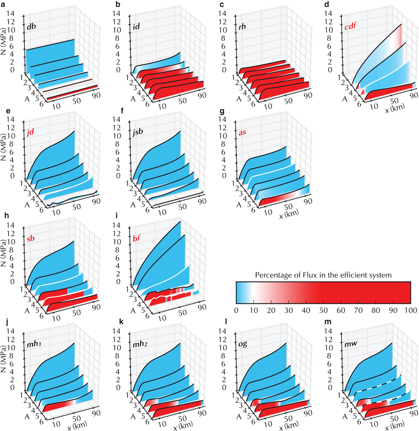
Fig. 2. Suite A results: mean value of the effective pressure (N) versus distance from the terminus (x) for all Runs (axis labelled A). Each submission is displayed in its own panel with the submission label printed. The results with the black and white dashed outline are the reference simulations used for tuning. Models that were tuned to any of the reference simulations have their submission name in red and the fitted Run(s) are highlighted with a white outline. The colours represent the level of channelisation of the drainage system. Here a shift from inefficient to efficient drainage system occurs when 10% of the total flux is drained by the efficient drainage system.
Table 2. List of symbols and fixed parameters used in the definition of the Suites of experiments

Table 3. Physical parameters appearing in the drainage model description with the values to be used, as applicable, for the simulations (Eqn (1)–(10), upper part)

Additional reference parameters from GlaDS-model (lower part).
Where the ice flow constant is for a closure relation as described in Eqn (5). equivalent Darcy--Weisbach f = 0.195 for semi-circular channel.
3.4. Suite A: steady state
The six Runs of Suite A are based on the ice-sheet topography (Eqn (11) and Fig. 1a) with a steady and spatially uniform water input. The primary objective of Suite A (beside providing a base-case for tuning) is to produce results for a simple steady state in terms of effective pressure and discharge. The input increases by four orders of magnitude from a low value corresponding to basal melt production (Run A1, m ≃ 2.5 mm a−1) to a high water input based on the peak water discharge driven by surface melt as observed in Greenland (Run A6, m ≃ 50 mm d−1 (Smith and others, Reference Smith2017), see Table 4).
Table 4. List of variable parameters for each Suite of experiment Runs. See the description of each Suite for more information on the parameters

3.5. Suite B: localised input
The importance of input localisation is investigated in Suite B. To test this, the spatially uniform input that was used in Run A5 is instead fed into an increasing number of moulins (i.e. point inputs). The number of moulins increases from one (B1) to 100 (B5) between which the discharge is equally partitioned (see Table 4). The location of the moulins is randomly generated for each Run and then used in all of the different models. Experimenters running 1-D models were instructed to collapse the moulins onto a single flowline. Additionally a distributed input, as in Run A1, is included to represent basal melt.
3.6. Suite C: diurnal cycle
The effect of short timescale dynamics, as represented by the diurnal melt cycle, on the response of the subglacial drainage system is targeted by Suite C. The starting point for the Runs of this Suite is the steady state achieved in Run B5 (steady input into 100 moulins). The different Runs are performed with diurnal melt cycles of increasing amplitude with recharge into each moulin given by
 $$R(t,R_a) = \max \left( {0,{\mkern 1mu} M_{in}\left[ {1 - R_a\sin \left( {\displaystyle{{2\pi t} \over {s_d}}} \right)} \right]} \right),$$
where t is the time in seconds, s d the number of seconds per day and M in = 0.9 m3 s−1 the background moulin input from Run B5 (see Table 4). The models were to be run until a periodic state was reached. The relative amplitude of the forcing R a ranges from 0.25 for Run C1 to 2 for Run C4 (see Table 4). For Run C4, the negative input values given by the high amplitude of the signal are cut off (see supporting Fig. S9) and this Run, therefore, has an overall higher water input than C1 to C3 (~20% of volume increase). As in B5, a uniform and constant background input equal to the recharge of A1 is applied.
3.7. Suite D: seasonal cycle
The long timescale (seasonal) evolution of the drainage system is investigated in Suite D. It uses initial conditions from Run A1, which represent the water input during winter. From this starting point, a seasonal cycle is applied to the water input and the model is run until a periodic annual state is achieved. The forcing is computed from a simple degree day model driven by a temperature parameterisation. The temperature at 0 m elevation is given by
 $${\rm T}(t) = - 16\cos \left( {\displaystyle{{2\pi t} \over {s_y}}} \right) - 5 + \Delta T.$$
The Runs of this Suite are achieved by increasing the mean annual temperature, the value of ΔT, from −4°C to 4°C (see Table 4).
The distributed recharge is then computed from the following degree day model formulation
 $$R(z_s,t) = \max \left( {0,{\mkern 1mu} DDF{\mkern 1mu} \left( {T(t) + z_s\displaystyle{{{\rm d}T} \over {{\rm d}z}}} \right)} \right),$$
where ((dT)/(dz)) = −0.0075 K m−1 is the lapse rate and DDF = 0.01/86400 m K−1 s−1 is the degree day factor (Table 2). As in Suites B and C, a uniform and constant basal melt input equal to that of A1 is applied in all Runs.
3.8. Suite E: overdeepening of valley topography
Suite E is designed to investigate the effect of bed slope on the models. The common base for this Suite is the synthetic valley topography (Eqn (12) and Fig. 1b). In the different Runs of this Suite the shape of the bed topography is altered to define a more or less pronounced overdeepening (Table 4 and Fig. 6k). The water input is constant and uniformly distributed at twice the rate of Run A6 (m ≃ 100 mm d−1). Note that reference parameters for the valley Runs results in a non-zero storage (Table 3).
3.9. Suite F: seasonal cycle on valley topography
Suite F runs a seasonal water forcing – mirroring Suite D – for the synthetic valley glacier using the baseline value of the topography parameter γ = γ b. First the models are run to a steady state with water input as in A1. This steady state is then used as an initial condition for all of the Runs. Following this, a seasonal forcing as specified with Eqn (16) and (17) is applied using temperature offsets between − 6°C and 6°C (Table 4).
4. RESULTS
The objective of this study is to illuminate the differences between various subglacial hydrology formulations to show how these differences affect model results. Our evaluation focuses on effective pressure as that is the principal coupling to ice dynamics, which, in turn, is a primary motivation behind subglacial drainage studies. All of the submitted results are open source and can be accessed at de Fleurian and others (Reference de Fleurian2018) for further investigation. We condense the results into three types of figures: steady state with distributed recharge (Suites A and E, Figs. 2 and 6), steady state with moulin input (Suite B, Fig. 3) and transient simulations (Suites C, D and F, Figs. 4, 5 and 7). Figs, 3, 4, 5 and 7 present only one or two Runs in detail on which we focus the discussion. However, the figures for the other Runs are provided in the supplementary material as well as numerous additional figures for each Run and model.
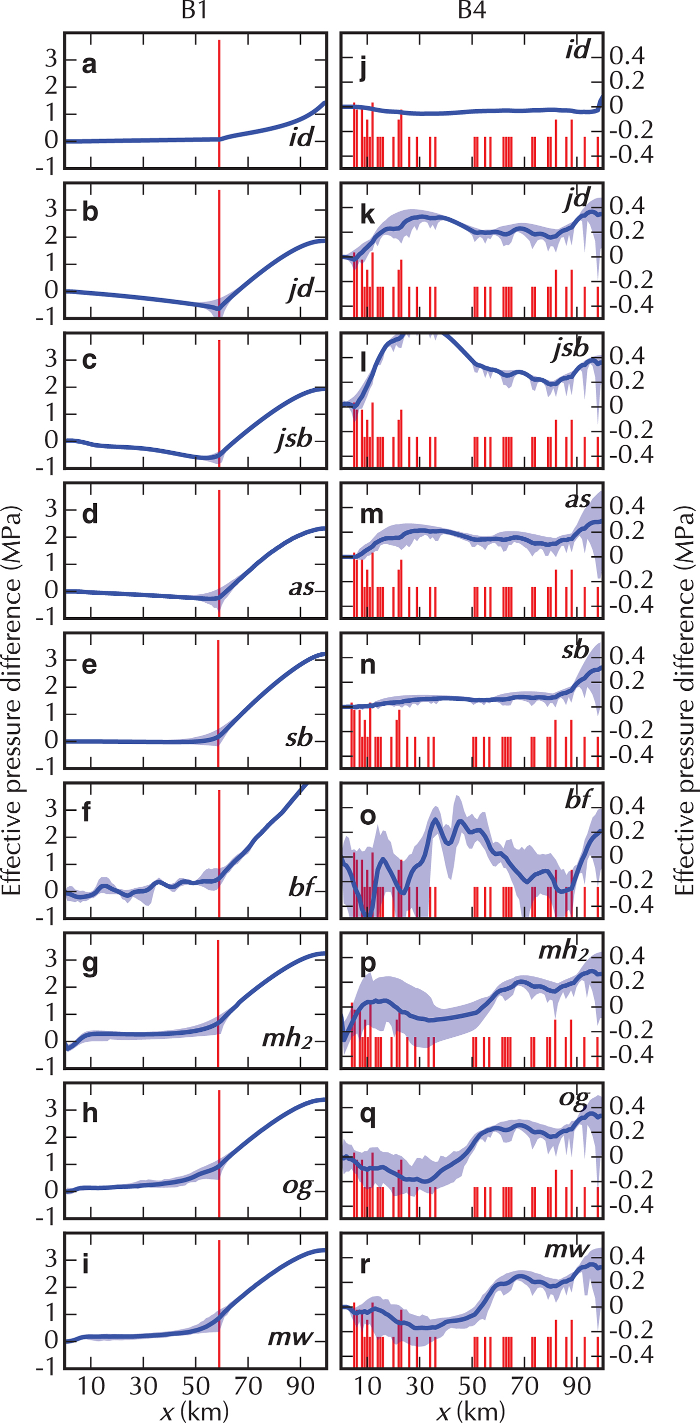
Fig. 3. Suite B results: the left column shows the difference in effective pressure between Run B1 and reference Run A5 (with same total recharge in both Runs). The right column shows the difference in effective pressure between Run B4 and A5. The differences are such that higher effective pressure in B yield positive values. The width-averaged difference is the solid blue line, and width-minimum and maximum difference are given by the light blue band. The red bars indicate moulin locations, their height scaled with the logarithm of input; the bars that are higher in Run B4 (right) are because multiple moulins are located at the same x-coordinate. Note that the scale of the effective pressure difference is different between the two columns.
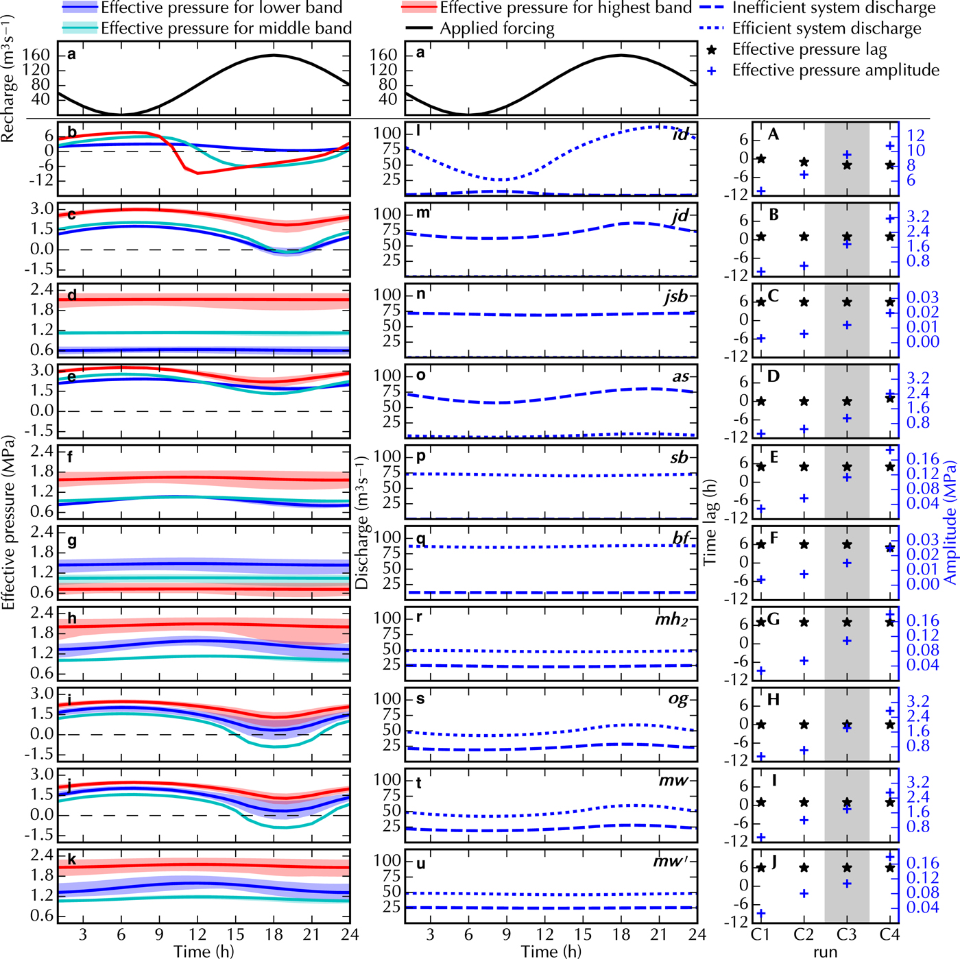
Fig. 4. Suite C results: left and centre columns show Run C3 with a panel for each submission, right column shows all Runs. The top row shows total recharge for the whole domain (a). Each row shows the results of one model (model label in the middle column). The left column (b to k) shows the evolution of the mean effective pressure in the three bands as defined in Fig. 1a. The coloured line shows the mean value and the shading represents the spread within the band. The dashed black line marks zero effective pressure. The middle column (l to u) shows the evolution of the discharge in the inefficient (dashed) and efficient (dotted) drainage system for the lower band. The right column (A to J) shows the time lag between maximum recharge and minimum effective pressure (black stars) and amplitude of the effective pressure variation (blue crosses) averaged over the entire domain for Runs C1 through C4. Note that the scale for amplitude of effective pressure variations varies between models. The greyed region in the right column identifies the Run plotted in the two left columns.
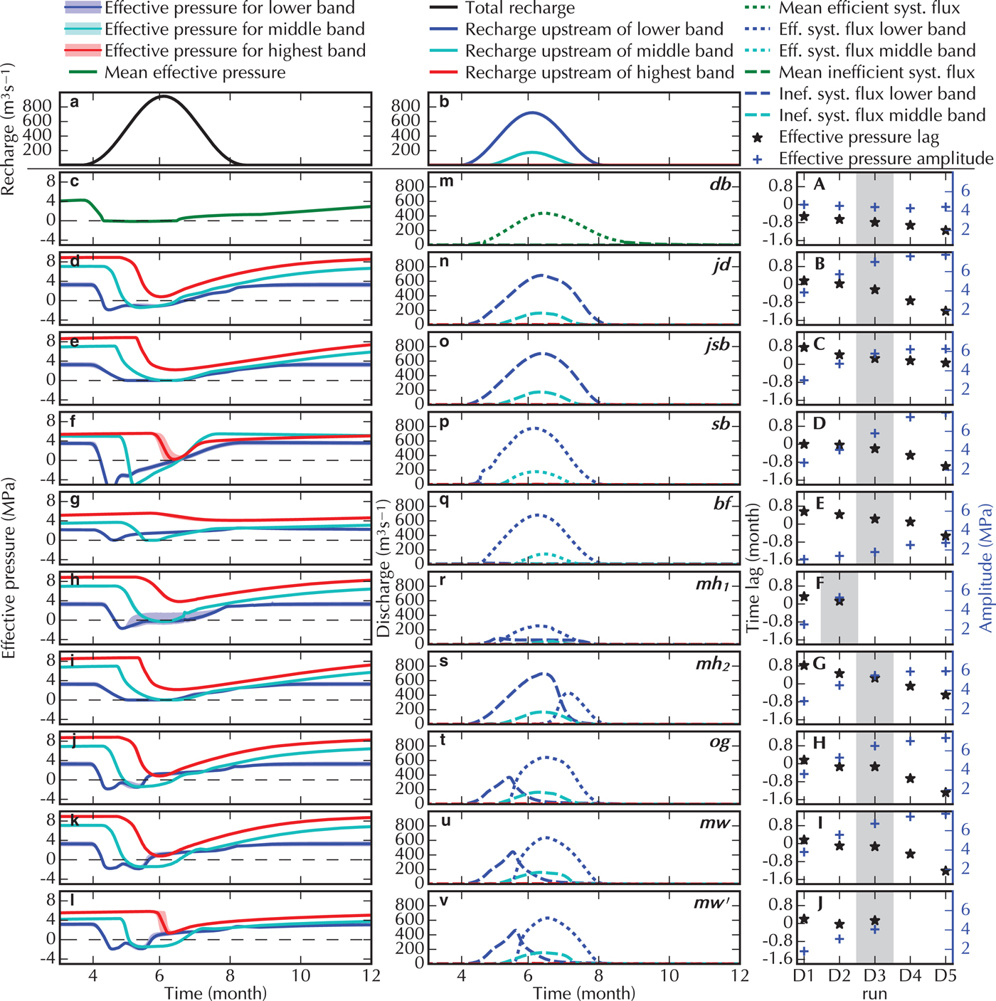
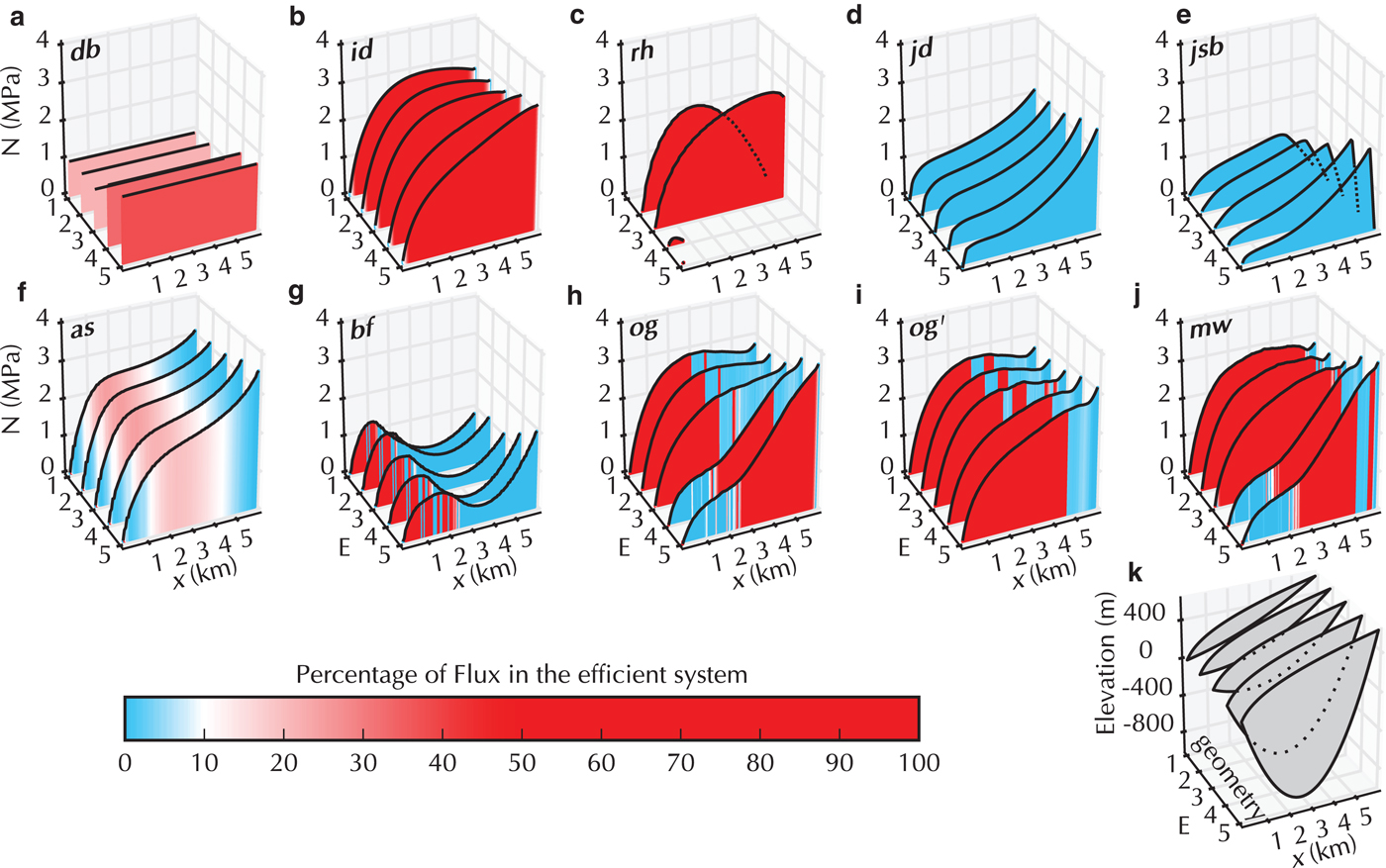
Fig. 6. Suite E results presented as in Fig. 2. The centreline topography used for each Run is shown in panel k. For the 2-D models, the effective pressure and the fraction of the flux in the efficient system are calculated by averaging values in a 200 m wide band along the centre-line (hatched band in Fig. 1b).
Steady-state Suites A and E (Figs. 2 and 6) are evaluated using the percentage of flux in the efficient system and the width-averaged effective pressure (N). The full width is used in Suite A and a band of 200 m width, indicated by the gray band in Fig. 1b, is used in Suite E. The former is calculated, in most models, as the ratio of width-averaged channelised flux to total flux. This ratio is straightforward to compute for models that calculate the flux separately in the two systems, but for models relying on a single system to model both efficient and inefficient drainage another quantity is used as a proxy: for sb, the flux is considered to pass through the efficient drainage system when the transmitivity is above 0.1 m2s−1; for as, db and id the ratio of melt opening rate to total opening rate is used; for jd, rh and jsb no proxy-quantity was calculated as they are single system models. In our analysis, we classify the drainage system as efficient if more than 10% of the discharge is through the efficient system; at this stage the effective pressure begins to be characteristic of an efficient system with increase in flux leading to increase in effective pressure.
We evaluate Suite B, also at steady state, by looking at the change between Runs B1 and B4, which use localised moulin input, as compared with Run A5, which uses the same total input but distributed uniformly (Fig. 3).
Suites C, D and F are transient models. Their width-averaged effective pressures are evaluated in three bands as displayed in Fig. 1 Their width-integrated discharge is evaluated in either the lowermost band (C) or all three bands (D,F) (Figs. 4, 5 and 7). Additionally, the phase lag is calculated between the recharge forcing and effective pressure signal, as well as the effective pressure amplitude.
4.1. Suite A: steady state
The effective pressure distribution and the type of system (inefficient in blue or efficient in red) is presented in Fig. 2. Moving upglacier from the terminus, all model Runs – except the lumped model db and those with an effective pressure close to zero on the whole domain – show a steep increase of effective pressure over the initial 10 km. This pressure distribution is driven by the ice-sheet geometry and the terminus boundary conditions. Farther upglacier, all of the model outputs follow the widely acknowledged rule that, in a steady state, a higher discharge leads to decreasing N if the system is inefficient and to increasing N if the system is efficient. This can be observed in Fig. 2 both as the discharge increases with proximity to the terminus, and as the specified recharge increases (from A1 to A6).
The different treatments of the subglacial drainage system lead to some variations in the results. The 0-D model db demonstrates channelisation in A5 but no corresponding increase in effective pressure either in A5 or the higher discharge A6. The channel and conduit models (rh and id, respectively) show a bias towards a more efficient drainage system, which is expected from their formulation. The effect of the single cavity of the conduit model id is clearly seen in A1 (and the upstream region in A2 and A3) where the effective pressure increases with a decrease in discharge. The channel (rh) and conduit (id) models also produce higher N for Run A6 than the fully channelised cavity-sheet/channels models (mh 2, og and mw), because all water is conducted through a single R channel, whereas the cavity-sheet/channels models have several parallel R channels (see supporting Figs. S145, S156, S177).
The cavity-sheet models (jd, jsb, as, mw, mh 1, mh 2 and og) show a shallow effective pressure gradient between 10 and ~70 km before it increases again near the upglacier domain boundary. Of those models, the ones using a cavity-sheet drainage system exclusively (jd and jsb), have lower effective pressure in the higher discharge Runs (A4-A6) compared with the models that also incorporate an efficient system. For the cavity-sheet model jd, the tuning to A5 does not yield significant improvement in the results of Run A6 (where the tuned values are used). The cavity-sheet model as produces effective pressure values positioned between those of the cavity-sheet and of the cavity-sheet/(one-)channel models, due to the inclusion of opening by melt across the entire domain, allowing efficient drainage to develop.
The models using tuning (cdf, jd, as, sb and bf) obtain a reasonable fit to their target input scenarios with a better fit for the higher input scenarios (when targeted). Using the tuned parameters, cdf and bf show effective pressures largely above that of the reference simulation mw for Runs A1 and A2 (or in the case of cdf, A3, as A1 and A2 did not converge in the cdf model), and show no shallow gradient region in the middle of the domain. Results from sb and cdf closely follow those of mw for Run A6 while bf did not converge for this Run. The porous-layer models sb and bf predict more channelisation for A4 than the reference results of mw. The different approaches to the porous approximation are particularly clear in this Suite where the single layer model allowing variations in transmitivity (sb) closely follows the results of mw with slightly lower effective pressure. Compared with this, the fixed transmitivity of the inefficient layer in bf model yield unrealistically large effective pressure under low water input.
4.2. Suite B: steady state with moulin input
Suite B examines the impact of localised recharge on effective pressure distribution. This is achieved by recharging the system through an increasing number of moulins while keeping a constant overall input. We show results for Runs B1 and B4 (Fig. 3), in which recharge is through one and 50 moulins, respectively (other Runs in supporting Figs. S1–5). Fig. 3 shows the difference in effective pressure between Run B1 and A5 in the left column, and that between Run B4 and A5 in the right column.
The results show two clearly different behaviours. In Runs B3 to B5, with 20, 50 and 100 moulins, respectively, the impact of the localised input on effective pressure is relatively small as can be seen in the example of Run B4 shown in Fig. 3j–r. All models that provided results for this Run show a similar response with the amplitude of the difference between A5 and B4 ranging from almost nothing for id to ± 0.5 MPa. In contrast, the lower moulin count Runs B1 and B2 (one and 10, respectively), produce distinctive spatial variability in their outputs (see B1 in Fig. 3a–i.). For those Runs, the largest difference from A5 is upstream of the highest moulin where the effective pressure increases, reaching values at least twice as large as that of A5 at the highest point of the domain. Downstream of the highest moulin, the pressure distributions are much closer to that of Run A5 with a maximum variation of ~10% of the ice overburden pressure. We attribute this pattern to the limited discharge, provided only by basal melt, upstream of the highest moulin. In general, in models with only an inefficient system, effective pressure is lower than in A5 below the uppermost moulin (negative values). The other models have higher effective pressure. It is interesting to note that the effective pressure drops locally at moulin locations in all 2-D models (Fig. 3b–i and k–r); this appears as small spikes along the lower bound of the pressure envelope (see also supplementary material).
4.3. Suite C: diurnal cycle
Suite C probes the time evolution of effective pressure and discharge in response to a diurnal meltwater forcing using the moulins of B5 as input locations (Fig. 4). Our discussion focuses on Run C3 and the other Runs are plotted in supporting Figs. S6–9.
The primary difference between the models is the magnitude of the simulated diurnal effective pressure variation (Fig. 4b–k), which is chiefly dependent on the amount of available englacial and/or subglacial water storage. Participants running a model including a storage component were instructed to set it to zero. However, many models require some amount of storage for numerical reasons and, therefore, retained non-zero storage for this Suite. Models with no storage (id, jd, as, og, mw) show large effective pressure amplitude and minimal lag (1–2 h) between maximum recharge and minimum N (Fig. 4A–J). This pressure amplitude increases with the forcing amplitude hence lowering the daily averaged effective pressure with respect to that of B5. Conversely, models including a storage component (jsb, sb, bf, mh 2, mw′) have a very small effective pressure amplitude and the lag is ~ 6 h. This leads to a daily mean value of the effective pressure that is close to the steady-state value of Run B5. The impact of available water storage amount is nicely illustrated by the two submissions of the same model mw and mw′, the former using no storage, the latter using storage (Fig. 4j,k). Note that the models jsb and mh 2 acquire their storage-like behaviour from solving a regularised pressure equation (Bueler and van Pelt, Reference Bueler and van Pelt2015) without actually storing water.
The same variations, or lack thereof, between storage and no-storage models also appear in the width-integrated discharge of the lower band (Fig. 4l–u). The cavity-sheet/channels models with little storage (og and mw) show a larger amplitude in the efficient system discharge, because the recharge via moulins directly feeds that system. The cavity-sheet/(one-)channel models (mh 2, og, mw and mw′) show a partitioning of the discharge with ~2/3 in the efficient and 1/3 in the inefficient system. In model as, most of the flux is through the inefficient system with a slight increase in efficient drainage when the recharge is at its maximum. Conversely, the two porous-layer models conduct most or all of the discharge in the efficient system.
4.4. Suite D: seasonal cycle
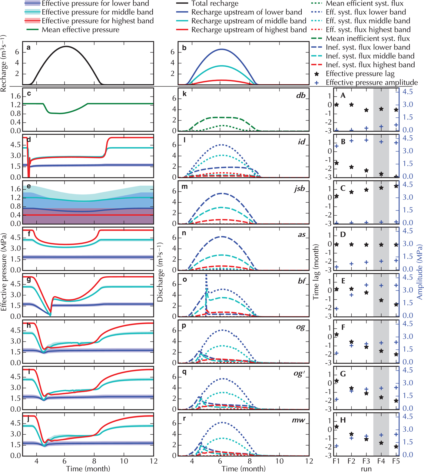
Suite D investigates the influence of seasonal forcing on the subglacial drainage system. This Suite uses a distributed recharge with increasing amplitude of the seasonal recharge from D1 to D5. We focus the discussion on the Run D3 (Fig. 5) which is presented similar to the results of Suite C. The other Runs of this Suite are plotted in supporting Figs. S10–14.
During winter, the effective pressure in all of the model Runs is ~3–8 MPa with lower N in the lower bands (first column of Fig. 5). This is in contrast to recorded winter pressures (e.g. van de Wal and others, Reference van de Wal2015), which tend to show effective pressures close to zero.
When the recharge increases in spring, the effective pressure drops in all models reproducing the commonly known spring event (Röthlisberger and Lang, Reference Röthlisberger and Lang1987), which propagates upstream and reaches the highest band (90 km from the front) by mid-summer. In some bands, the models that do not cap N at zero obtain negative effective pressures, in many instances persisting for several months, during this phase. For all of the models aside from the double porous-layer (bf), the amplitude of the effective pressure drop is similar over the whole domain, whereas the bf model shows a notably smaller amplitude in the highest band of the domain.
The different models recover from this spring event in different ways. The main difference is the ability of the two-components model to develop an efficient system, which is observed on the distribution of the discharge between the two systems (middle column Fig. 5). The cavity-sheet/(one-)channels models initially carry most of the discharge in the distributed system before transitioning – but only in the lower band – to channelised drainage. The mh 2 model shows a later transition than the other three cavity-sheet/channels models (og, mw, mw′). The cavity-sheet/one-channel model (mh 1) still discharges a sizeable amount of water through its inefficient system when the channel is active (see supporting Fig. S11 to compare D2 Runs). For the double porous-layer model (bf) and the single component models where a threshold is fixed to define efficient drainage (db and sb), the shift to efficient drainage occurs earlier in the season compared with the cavity-sheet/(one-)channels models. This shift is also more widespread, reaching as high as the middle band where the cavity-sheet/(one-)channels models show an efficient drainage only in the lower band. The cavity-sheet models show an asymmetric discharge with an increase that is slower than the recharge increase and a steeper discharge decrease at the end of the melt season.
The results of the higher storage Run mw′ (compared with mw) indicate that higher storage leads to a lower effective pressure during winter and a delayed drop in the effective pressure in the highest band (red). Similar outputs occur with the porous layer models (sb and bf), but not with the models using storage as a means of stabilisation (jsb and mh 2).
The rightmost column of Fig. 5 shows the amplitude of the effective pressure variations and the time lag between the time of maximum recharge and minimum effective pressure for all D Runs. All models show similar trends for those two values: the effective pressure minimum occurs earlier as the water recharge increases (from D1 to D5). For most models, the effective pressure minimum follows peak recharge with lower recharge intensities, and precedes peak recharge with higher recharge intensities. The amplitude of the effective pressure variation also increases as discharge increases, except in the 0-D model (db). The latter is because the effective pressure in model db is restricted to positive values, thus limiting the amplitude of the response already for Run D1.
4.5. Suite E: overdeepening of valley topography
Suite E tests the influence of an overdeepening on the simulated steady-state drainage system (Fig. 6). This Suite is performed with the synthetic valley glacier topography shown in Fig. 1b. The main impact of an overdeepening should come through the pressure dependence of the melt-opening term (second term of Eqn (7)), which at the supercooling threshold (e.g. Werder, Reference Werder2016) should lead to shutdown of R channels. The overdeepenings in the topography for Runs E1 to E3 are not sufficient to reach the supercooling threshold. This threshold first appears in the geometry for Run E4.
The R channel shutdown is seen in the channel model rh: for Run E3 the model produces positive effective pressures throughout; however, for E4 the model channel shuts down at ~1 km and N drops to 0, at which point the model fails. The id model has similar physics as rh but does not include the pressure-melt term in Eqn (7). Consequently, the overdeepening has very little influence on the shape of the effective pressure curve as the (constant) surface slope is then the dominating influence.
Similarly, the cavity-sheet models jd and jsb that have no pressure-melt dependence (Eqn (5)), show little impact of the overdeepening, producing positive effective pressures throughout. The pronounced difference between jd and jsb, particularly towards the upper glacier, is due to the fact that the jsb model constrains water pressure to always be positive. This means that effective pressure has to go to zero at all boundaries (where ice thickness is zero), including the upper glacier margin. All other 1-D and 2-D models that submitted results for Suite E (and F) ignore such constraints and generally produce negative water pressures in part of the valley glacier domain (see supplementary material). The as model, which is also a cavity-sheet model but includes opening by melt and a pressure dependent term, shows small effects due to the overdeepening. The different discharge formulation used in this model allows for representation of laminar and turbulent flow regimes, as well as the wide transition between them, producing smooth transitions between inefficient and efficient systems. As the topography deepens, more of the bed is in a flow regime closer to laminar (i.e. lower Reynolds number, with linear dependence on potential gradient). This represents weakening of efficient system (or channel shutdown) as the overdeepening becomes deeper, and is apparent in the extension of the downstream blue region (inefficient system) from E1 to E5 in Fig. 6f.
The cavity-sheet/channels models (og and mw) show no negative effective pressures, unlike rh, even though they do contain the pressure-melt term. However, N is reduced markedly in Runs E4 and E5, in which the supercooling threshold is exceeded and in the same region the drainage system transitions from efficient for x > 2 km to inefficient for 0 < x < 2 km. This means that the channel system does shut down and that the water is then carried in the cavity-sheet (and also in channels along the sides of the overdeepening, e.g. compare supporting Figs. S162 and S166). og′ is similar to og but the pressure-melt term is turned off. This model, again, therefore shows very little impact of the overdeepening and the efficient system operates over the full length of the glacier.
The porous-layer model bf shows a pronounced impact of the valley topography, N changes only slightly as the overdeepening is enlarged, so the bed topography has little impact. The model suggests that an efficient drainage system would exist between the margin and x = 2 km, transitioning to an inefficient system at x > 2 km. This causes the effective pressure to drop to a minimum at x = 4 km.
For the 0-D model (db), which has no pressure-melt term, the effective pressure is similar for the first three Runs and then rises slightly for the last two. This is unlike the other models, which all show a decrease in effective pressure (albeit only a small one when there is no pressure-melt term). This effect may be caused by the use of an averaged topography in this lumped model.
4.6. Suite F: seasonal cycle on valley topography
Suite F has the same objective as Suite D – to explore the seasonal drainage cycle – but with the valley-glacier topography of E1, without an overdeepening (Fig. 1). The results are presented in the same style as Suites C and D with the discussion focusing on Run F4 (Fig. 7 and supplementary material).
During winter, the effective pressure in all models is relatively high and markedly higher than during times of meltwater input (left column). The lowest N is produced by the jsb model, particularly at the highest elevation. This is again because this model constrains the water pressure to be positive, as mentioned above. This is also why the spread in effective pressures in the jsb model is the largest of all models (light coloured bands in Fig. 7e), as N is forced to zero at the lateral margins. All other models have very little lateral spread in effective pressure and they yield negative water pressures towards the margins.
As in Suite D, the models approximate a spring event when recharge sets in. However, in the case of this geometry, there are larger variations in the shape of the pressure drop and its subsequent recovery. The 0-D model db and the cavity-sheet models as and jsb show a gradual decrease in effective pressure. The ample water storage in model jsb explains this smoother evolution, while the low discharge through the efficient system of as model clarifies the evolution of its effective pressure. For the conduit model, id, the effective pressure response drops sharply in all elevation bands. This is followed by a rapid recovery to a steady summer value. The cavity-sheet/channels models og, og′ and mw show a pronounced drop over about 1 month with a slight recovery after channelisation initiates (see discharge plot in middle column of Fig. 7). These models then enter a summer mode in which the effective pressure rises slowly and steadily during the melt season. The porous-layer model, bf, shows a more gradual drop to almost zero effective pressure and then a rapid recovery as the efficient layer is activated. This is also clearly visible in the discharge plots.
At the end of the summer, the return to the winter state happens at different rates. In models db, id, as and bf the return occurs simultaneously with recharge shutdown. The cavity-sheet/channels models og, og′ and mw and the cavity-sheet model jsb recover much more slowly over the course of a few months. Notice, too, that in the cavity-sheet/channels model og, og′ and mw, there is a clear difference in the slope of the effective pressure between the summer regime and the return to the winter state at the end of the melt season.
The dynamic response to the different magnitudes of forcings Runs F1--F5 (right column), shows that in most models the time of minimum effective pressure (taken as an average over the whole domain) leads the time of maximum recharge by ~1 month; this lead time increases with recharge intensity. Similarly, the amplitude of the effective pressure increases with increased forcing. Exceptions to this are: jsb, for which effective pressure lags recharge and the amplitude stays very low; and as, which shows an increasing amplitude but zero lag, because zero storage is used by this model in this Suite.
5. DISCUSSION
The SHMIP exercise consists of six Suites of four to six Runs each. The Suites are designed to facilitate a comparison of several different models of the subglacial drainage system. The experiments were designed to enable participation of a wide variety of models, with the only requirement being that the effective pressure was computed. This excluded some models, notably the routing-type models which use a hydraulic potential (and thus effective pressure) that is independent of the state of the drainage system (e.g. Le Brocq and others, Reference Le Brocq, Payne, Siegert and Alley2009); as well as the models that only consider local water balances, such as subglacial till models (e.g. Tulaczyk and others, Reference Tulaczyk, Kamb and Engelhardt2000; Bougamont and others, Reference Bougamont2014). Nonetheless, our publicly available results could be re-interpreted in terms of discharge only and compared with outputs of those types of models.
To allow a comparison of models with different physical approaches, two reference simulations are provided. This allowed participation of models requiring tuning. The choice of the reference Runs (ice-sheet geometry, steady state and uniform input Runs A3 and A5) is such that fitting to these results should not bias the rest of the intercomparison, in which simulations with different characteristics are presented. Likewise, the choice of a cavity-sheet/channels model for this reference simulation (mw) is motivated by the fact that this approach is the most widespread and therefore these reference models give a set of parameters for the bulk of existing models. The tuning procedure (or need for tuning) was left to the discretion of the experimenter and was not a mandatory step of the intercomparison. Note that models that are tuned use parameter values that are similar to those used in other studies conducted with these same models.
The 13 participating models show a broad agreement between each other in all Suites. In particular, they agree with one of the fundamental theoretical considerations of subglacial drainage: in an inefficient drainage system a discharge increase will lead to a decrease in steady-state effective pressure and conversely, in an efficient drainage system, a discharge increase will lead to an increase in steady-state effective pressure (Fig. 2). Conversely, none of the models produce the low effective pressure that is usually observed during winter (e.g. Wright and others, Reference Wright, Harper, Humphrey and Meierbachtol2016). The more specific responses of the models are generally comparable across groups of models incorporating similar physics (see ‘Model type’ in Table 1). In view of the complexity in analysing and interpreting the published subglacial hydrology records (e.g. Rada and Schoof, Reference Rada and Schoof2018), our discussion of the SHMIP results focuses primarily on an intercomparison of the model outputs. A direct comparison with observations is beyond the scope of this study and is left to a future SHMIP.
A large number of models use a cavity-sheet drainage system (jd, jsb, as, mh 1, mh 2, og, mw), which leads to consistent results for all of these in low recharge scenarios (A1–A3, winter period of D and F). The 0-D conduit model db also produces results consistent with the cavity-sheet models for those scenarios. The other models show different behaviours at low recharge: the two layered porous-layer models (bf) as well as macroporous-sheet model (cdf) produce much higher effective pressures than the cavity-sheet models. This is because the conductivity of the inefficient drainage system in these models does not adapt to the discharge of the system. Conversely, the 1-D channel or conduit models (rh, id), which are designed for higher recharge scenarios, show much lower effective pressure at low discharge, which is consistent with R channel. The scaling of the transmitivity to a cavity opening formulation in the single layer porous model (sb) allows a reduction in the layer conductivity at low discharge yielding effective pressure distributions closer to those of mw.
For higher recharge Runs, the response of the models with and without an efficient drainage component diverge as can be seen in Suite A (Run A4--A6) and E1 and E2 (which have no overdeepening). Notably, the representation of the efficient drainage system in the porous-layer models seems to capture the dynamics observed in the cavity-sheet/channels models for Suite A rather well. However, although the differences between cavity-sheet-only and cavity-sheet/channels models are large for the steady-state Runs (Suites A, B and E), they are much smaller for seasonal forcings (Suites D and F). For example, jd is very similar to mw in Suite D except in the band closest to the margin (10–15 km, Fig. 5). The likely cause of this is that the transient ‘summer’ states in Suites D and F are far from a steady-state channelised system. This means that in those seasonal Runs the distributed system drains more of the subglacial discharge than it would in a steady state corresponding to a high magnitude summer recharge. This interpretation can be supported by field measurements. Based on borehole observations in a land-terminating area of the Greenland ice sheet, Meierbachtol and others (Reference Meierbachtol, Harper and Humphrey2013) suggested that channels do not reach further inland than ~20 km. In the same region, tracer experiments suggest that the channelised system extends inland at least 41 km but not as far as 57 km (Chandler and others, Reference Chandler2013).
The impact of topography on steady states can be seen by comparing results of the high recharge Runs of Suite A (A5, A6) with the Run E1 (or E2) of Suite E, in which there is no overdeepening and recharge is similar. The channel models (db, id, rh, og, mw) produce about double the values of effective pressure in E1 versus A6 (e.g. id in Fig. 2b vs. Fig. 6b). This is due to the steeper surface slopes and shorter glacier length in the valley domain. Similarly, the cavity-sheet-only models (jd, jsb, as) produce effective pressures near zero in A6, whereas in E1 they are ~ 1 MPa, again due to the influence of topography.
The moulin-recharge Suite B illustrates that the impact of localised input on average effective pressure is relatively minor in all models, with variations usually <10% of the ice overburden pressure. However, there is one exception: it matters where the upper moulin is located, as above that moulin the effective pressure is much higher than predicted by a uniform input. The farthest inland location where water reaches the glacier bed is indeed a topic of current studies (e.g. Poinar and others, Reference Poinar2015; Gagliardini and Werder, Reference Gagliardini and Werder2018; Hoffman and others, Reference Hoffman2018a). Introducing localised inputs also modifies the local effective pressure (with lower effective pressure at the moulin locations) and the distribution of the efficient channelised drainage system (see supplementary figures). This decrease of effective pressure at moulin locations is consistent with observations that hydraulic head is higher in the vicinity of moulins (Gulley and others, Reference Gulley2012; Andrews and others, Reference Andrews2014).
The transient Runs illustrate the importance of storage (in the sense of a direct functional relationship between pressure and storage as in Eqn (10)) and also of storage-like effects that can arise from numerical regularisation. In the diurnal-variation Suite, C, storage impacts the amplitude of the pressure variation, with results ranging from almost zero (high storage) to 13 MPa (no storage) (Fig. 4). These amplitudes can be compared with observations from Haut Glacier d'Arolla (Gordon and others, Reference Gordon1998), where amplitudes varying from 0 to 0.9 MPa were observed in a cluster of boreholes. Note that two models, jsb and mh 2, do not implement actual storage but use a storage-like term to regularise the pressure equation (see Bueler and van Pelt, Reference Bueler and van Pelt2015). This results in some of the same effects as actual storage. The discharge also has a muted diurnal variation, compared with recharge, as storage increases. Therefore, observations of recharge and proglacial discharge could help further constrain the storage capacity of a glacier drainage system (e.g. Huss and others, Reference Huss, Bauder, Werder, Funk and Hock2007; Bartholomew and others, Reference Bartholomew2012; Brinkerhoff and others, Reference Brinkerhoff, Meyer, Bueler, Truffer and Bartholomaus2016).
For the seasonal forcings (Suites D and F), storage has a lesser impact as the drainage system has more time to react to the more gradually changing recharge. In the mw model, increasing storage (mw′) leads to lower effective pressure during the winter and also to a delayed but sharper response in spring in the two higher elevation bands. The former is due to increased water flow (and thus lower N) during winter as more water can be released from storage. The latter is due to the dampening effect that increased storage has on the subglacial water pressure response.
The seasonal-forcing Runs of all models produce an effective pressure that is high, higher, in fact than at any time during the melt season (except for the porous-layer models in the highest elevation band in Suite D, Fig. 5f,g). This is contrary to many borehole observations (e.g. Fudge and others, Reference Fudge, Harper, Humphrey and Pfeffer2005; Dow and others, Reference Dow, Kavanaugh, Sanders, Cuffey and MacGregor2011; Rada and Schoof, Reference Rada and Schoof2018), which show a shutdown of the drainage system leading to effective pressures around zero. There has been some recent progress in modelling such a shutdown (Hoffman and others, Reference Hoffman2016; Dow and others, Reference Dow, Karlsson and Werder2018; Downs and others, Reference Downs, Johnson, Harper, Meierbachtol and Werder2018; Rada and Schoof, Reference Rada and Schoof2018) but none of the participating models include such processes. An alternative view is that the participating models, as well as many others, only simulate a well-connected system which could potentially persist at high effective pressures throughout the winter with a footprint, however, small enough that it is rarely observed.
All the models show pronounced ‘spring events’, with low effective pressure as the surface melt forcing sets in (Iken and Bindschadler, Reference Iken and Bindschadler1986), in both Suites D and F. The effective pressure then increases again as the drainage system adjusts to the higher flux. Of note is that this increase in effective pressure also occurs in models with only an inefficient system, such as jd (Fig. 5d). This is because an inefficient system will also (transiently) respond to an increase in recharge with an effective pressure drop and a subsequent rise as the drainage space and thus the efficiency increases Eqn (4), as explained in Hoffman and Price (Reference Hoffman and Price2014). The duration of the effective pressure drop varies from less than a month to several months. These pressure drops are consistent with observed speed-up events ranging from one to several months depending on the location of the measurements (Bartholomew and others, Reference Bartholomew2010; Hoffman and others, Reference Hoffman, Catania, Neumann, Andrews and Rumrill2011; van de Wal and others, Reference van de Wal2015).
Most models reach negative effective pressures in Suite D for extended periods of time in both the lower and middle band. The models that do not reach negative N either constrain it to be positive (db, jsb, mh 2) or, in the case of bf, instantly activate the efficient drainage system when N = 0 is reached (this activation can be seen nicely in Fig. 7o). A positive N is arguably a more realistic behaviour as month-long periods of negative effective pressures over the large areas predicted by the other participating models is not observed and would have a much more dramatic impact on ice dynamics than ‘spring events”. However, probably none of the models capture the drainage system dynamics correctly as N approaches zero, as then uplift of the ice, including non-local effects due to elastic and viscous behaviours, should occur (Tsai and Rice, Reference Tsai and Rice2010; Walker and others, Reference Walker, Werder, Dow and Nowicki2017). Note that in the seasonal Suite, F, zero or negative effective pressures are reached only very briefly by bf and id. All others models have N > 0.7 MPa. Again this is due to the larger surface slopes and shorter length of the valley topography compared with the topography of Suite D.
The simulated transitions back to the winter state at the end of the melt season are of varying temporal length. The porous-layer models recover very quickly, in less than a month for Suite D and even more rapidly for F, afterwards the effective pressure only increases slightly. The cavity-sheet models, in addition to the 0-D-conduit model, db, react much more slowly. In Suite D they transition to the winter state over 3--4 months. The large-scale effective pressure considered in SHMIP (mean value over an altitudinal band rather than local effective pressure) is not necessarily suited for direct comparison with observations. However, the idea of different ‘stages’ (Rada and Schoof, Reference Rada and Schoof2018) is particularly helpful. The transition of effective pressure back to its winter level can be compared with ‘stage 2’, which lasts around a month and is approximately represented in our seasonal Suite F for the valley glacier topography. This result, however, depends on the interpretation of both the model results and the field observations and will be open for debate until more efficient ways to compare modelled and measured effective pressure are developed.
Of the participating models, the most physically complex models are the cavity-sheet/channels models. They largely reproduce theoretically expected behaviours as explained above. This is why we picked the outputs of such a model as tuning benchmarks (Runs A3 and A5 of mw). The models that used this tuning were the ones which use implementations based on different draining components: the macroporous-sheet model (cdf), the porous-layer models (sb, bf), a cavity-sheet model including energy dissipation (as) and another cavity-sheet model (jd) in only a subset of the experiments. None of the participating models incorporated physically-based theories of drainage other than cavity(-sheets) and R channels. Thus, models involving canals (Walder and Fowler, Reference Walder and Fowler1994) or other distributed drainage types (e.g. Creyts and Schoof, Reference Creyts and Schoof2009) are not represented.
Models that implement only a cavity-sheet show shortcomings when applied to higher input scenarios, producing effective pressures that are too low. However, in the seasonal Runs, which are likely the most realistic forcings in this intercomparison exercise, they are not much different from the cavity-sheet/channels models even though recharge is high in mid summer. This high input can, in the case of these cavity-sheet only models, be accommodated by the increase in efficiency of the cavity-sheet system. This shows that they are probably applicable to many situations. However, they lack the fast rebound of the effective pressure in their frontal region, which might be quite relevant for ice dynamics (e.g. van de Wal and others, Reference van de Wal2015). On the other hand, they benefit from less model complexity and from a clearer mathematical foundation, in the sense that they approximate a continuum solution (Bueler and van Pelt, Reference Bueler and van Pelt2015). The as model gains wider applicability by introducing the pressure melting-opening term (e.g. Run A6). The momentum equation used in this model facilitates the transition between flow regimes, thus allowing the process of self-organised channelisation to occur stably, while including the melt term everywhere (Sommers and others, Reference Sommers, Rajaram and Morlighem2018). Previous model formulations found the inclusion of a melt term to be problematic (Schoof and others, Reference Schoof, Hewitt and Werder2012) albeit possible (Dow and others, Reference Dow, Karlsson and Werder2018).
The porous-layer models yield results that are similar to those of the cavity sheet/channels models for many of the Suites. The sb model is able to generate quite complex effective pressure variations with a single layer model. The double layer approach of bf is applicable to the steeper valley glacier topography and produces a response comparable with that of the cavity sheet/channels models in Suite F.
The results from the 0-D, conduit model (db) show that simplification can be pushed far. The overall behaviour of the model is qualitatively in line with the more complex cavity sheet/channels models. However, the results of this model are biased toward lower effective pressure and compare better to values in the lower region of the domain than to the overall mean value of the spatially distributed models. This could be due not only to the design of the model itself, but also to the chosen parameterisation or chosen topography. Also notable is the fact that the db model is one of the few subglacial drainage models that has been rigorously fit to observations using Bayesian methods (Brinkerhoff and others, Reference Brinkerhoff, Meyer, Bueler, Truffer and Bartholomaus2016); most other models have only been hand-tuned (if at all) to fit observations (e.g. de Fleurian and others, Reference de Fleurian2016; Koziol and Arnold, Reference Koziol and Arnold2018).
The three 1-D models (rh, cdf, id) show results consistent with the theories they implement. Their shortcomings are likely related more to approximations of the theory than to the fact they are implemented in only one dimension. This is in part due to the fairly 1-D geometries of our test Suites. The performance of these models suggests that 1-D models are valuable in settings where geometry can be reduced to a flow line with insignificant lateral variation.
6. CONCLUSION
Thirteen models participated in this first SHMIP. They incorporate a wide range of different drainage system types, with a focus on inefficient drainage through linked-cavities, efficient drainage through R channels and approximations of both of these systems by using drainage through porous-layers. All participating models were required to calculate effective pressure distributions. Models incorporating other physically based theories of drainage such as canals (Walder and Fowler, Reference Walder and Fowler1994) or other distributed drainage types (e.g. Creyts and Schoof, Reference Creyts and Schoof2009) did not participate. Routing models were excluded because they fail to compute effective pressure, which is a diagnostic variable in our tests
The test Suites of SHMIP cover a range of scenarios similar to those to which subglacial drainage models are currently applied. The Suites use synthetic, idealised topographies of a land-terminating ice-sheet margin and a mountain glacier, with idealised recharge forcing, ranging from steady input to seasonal and diurnal variations. However, a few interesting and relevant scenarios are not included, such as the classic test case of jökulhlaups (e.g. Nye, Reference Nye1976; Clarke, Reference Clarke2003; Flowers and others, Reference Flowers, Bjornsson, Palsson and Clarke2004). A tidewater glacier test-case is also missing, although such a case would be interesting in both Greenland-like and Antarctica-like scenarios (e.g. Dow and others, Reference Dow, Werder, Nowicki and Walker2016). Considering realistic modelling, some more complex forcings, such as a seasonal forcing with superimposed diurnal variations, and also real glacier topography would be of interest. These will be useful test targets to be included in a future iteration of SHMIP.
This intercomparison project provides a qualitative comparison of several state-of-the-art and legacy subglacial hydrology models. The use of a two-component model is strongly advised when considering high recharge scenarios, complex topographies, or observing short-term variations in the subglacial hydrological system. For larger systems with low water fluxes, the use of a cavity-sheet only model should be considered as they achieve results comparable with more complex cavity-sheet/channels models. These cavity-sheet/channels models are required when the dynamics of the efficient system is important, as in valley glaciers, or when recharge is constant enough to let channels develop. Porous layer models are a viable approximation to the more physically realistic approaches in that they capture, qualitatively, the inefficient and efficient system dynamics, but a careful assessment of their parameters and flux formulations should be performed to ensure that they accurately represent the flow regime corresponding to the recharge applied to the model.
This intercomparison reveals that the effect of localised drainage is important on small scales but does not have a significant impact on the overall distribution of water pressure. However, special care should be taken when specifying the location of the highest-altitude input point, as this altitude has a significant effect on the subglacial water pressure downstream.
Experiments introducing diurnal and seasonal variations emphasise the impact of water storage on the results of the models and more particularly on the timing of their response in terms of pressure. This could enable the parameterisation of storage from observations of the lag between water input and pressure response, and also put a constraint on models which introduce storage as part of their equations (e.g. the porous layer models) or as a stabilisation mechanism (e.g. as in mh 1).
Another well-known and important point, also highlighted by this exercise, is the need to use appropriate model parameters. However, these parameters are often largely unknown and future efforts should focus on inferring them from observations (e.g. Werder and others, Reference Werder, Schuler and Funk2010; Brinkerhoff and others, Reference Brinkerhoff, Meyer, Bueler, Truffer and Bartholomaus2016), or through other means such as laboratory experiments. Once these techniques of parameter inversion of subglacial drainage models become more established and reliable, a SHMIP exercise using observational data will become viable.
7. CONTRIBUTION STATEMENT
B.dF. and M.A.W. designed the experiments, ran their respective models, analysed the model results and wrote the paper. All the other co-authors ran their respective models and provided feedback both on the intercomparison design and paper writing.
SUPPLEMENTARY MATERIAL
The supplementary material for this article can be found at https://doi.org/10.1017/jog.2018.78
ACKNOWLEDGMENTS
B.dF. and M.A.W. want to thank everyone that took part in the discussions leading to SHMIP (Tim Creyts, Ian Hewitt, Christian Schoof, Gwenn Flowers, Jesse Johnson, Ed Bueler, Ugo Nanni, Angelika Humbert, Alison Banwell, Ian Willis, Stephen Price and others).
B.dF. was supported by the European Research Council under the European Community 7th Framework Programme (FP7/2007–2013)/ERC under Grant Number 61 0055 (ICE2ICE) and computations were performed on resources provided by UNINETT Sigma2 – the National Infrastructure for High Performance Computing and Data Storage in Norway.
S.B. was supported by the GreenRISE project, a project funded by Leibniz-Gemeinschaft: WGL Pakt fr Forschung SAW2014-PIK-1. I.D. was supported by the Swiss National Science Foundation (SNSF) National Research Programme (NRP) 70 ‘Energy Turnaround’, Project No.153927. C.D. was supported by the Canada Research Chairs Programme and the Natural Sciences and Engineering Research Council of Canada (Discovery – RGPIN-03761-2017).
J.D. wants to thank Jesse Johnson for his help in implementing the model, he was funded for this work by NSF grant 1543533. O.G. was supported by the Agence Nationale pour la Recherche (ANR) through the SUMER project (Blanc SIMI 6-2012).
M.J.H. was supported by the Laboratory Directed Research and Development Early Career Research Program at Los Alamos National Laboratory (20160608ECR). J.S. was supported by the Swiss National Science Foundation (SNSF) grant no. 200021-153179/1 to M. Funk and the Swiss National Supercomputing Centre (CSCS) allocation no. s573 to J. Seguinot.
A.S. was supported primarily by a NASA Earth and Space Science Fellowship (NNX14AL24H), and thanks Harihar Rajaram and Mathieu Morlighem for their invaluable contributions to model formulation and development. The authors want to thank two anonymous reviewers and the editor F. Pattyn for constructive comments that help to improve this manuscript.


 Open access