the Creative Commons Attribution 3.0 License.
the Creative Commons Attribution 3.0 License.
Spatial and temporal distributions of surface mass balance between Concordia and Vostok stations, Antarctica, from combined radar and ice core data: first results and detailed error analysis
Emmanuel Le Meur
Olivier Magand
Laurent Arnaud
Michel Fily
Massimo Frezzotti
Marie Cavitte
Robert Mulvaney
Stefano Urbini
Results from ground-penetrating radar (GPR) measurements and shallow ice cores carried out during a scientific traverse between Dome Concordia (DC) and Vostok stations are presented in order to infer both spatial and temporal characteristics of snow accumulation over the East Antarctic Plateau. Spatially continuous accumulation rates along the traverse are computed from the identification of three equally spaced radar reflections spanning about the last 600 years. Accurate dating of these internal reflection horizons (IRHs) is obtained from a depth–age relationship derived from volcanic horizons and bomb testing fallouts on a DC ice core and shows a very good consistency when tested against extra ice cores drilled along the radar profile. Accumulation rates are then inferred by accounting for density profiles down to each IRH. For the latter purpose, a careful error analysis showed that using a single and more accurate density profile along a DC core provided more reliable results than trying to include the potential spatial variability in density from extra (but less accurate) ice cores distributed along the profile.
The most striking feature is an accumulation pattern that remains constant through time with persistent gradients such as a marked decrease from 26 mm w.e. yr−1 at DC to 20 mm w.e. yr−1 at the south-west end of the profile over the last 234 years on average (with a similar decrease from 25 to 19 mm w.e. yr−1 over the last 592 years). As for the time dependency, despite an overall consistency with similar measurements carried out along the main East Antarctic divides, interpreting possible trends remains difficult. Indeed, error bars in our measurements are still too large to unambiguously infer an apparent time increase in accumulation rate.
For the proposed absolute values, maximum margins of error are in the range 4 mm w.e. yr−1 (last 234 years) to 2 mm w.e. yr−1 (last 592 years), a decrease with depth mainly resulting from the time-averaging when computing accumulation rates.
Please read the corrigendum first before continuing.
-
Notice on corrigendum
The requested paper has a corresponding corrigendum published. Please read the corrigendum first before downloading the article.
-
Article
(3438 KB)
-
The requested paper has a corresponding corrigendum published. Please read the corrigendum first before downloading the article.
- Article
(3438 KB) - Corrigendum
- BibTeX
- EndNote


The surface mass balance (SMB) over the Antarctic ice sheet is of primary interest for many purposes. The mass budget of the Antarctic ice sheet can be seen as the difference between all mass exchange with the atmosphere over all the ice sheet surface (i.e. the SMB) minus the calving of icebergs and basal melting under ice shelves at the coast. The first term is globally positive as it represents snow accumulation over most parts of the ice sheet with the exception of blue ice and wind crust areas with negative SMB due to wind scouring and/or sublimation (Bintanja, 1999; Scambos et al., 2012). The second is negative despite the possibility of marine ice accretion under some parts of the shelves. Although current changes in the mass budget of Antarctic ice are believed to result mainly from recent dynamical effects leading to an enhanced flow of ice through outlet glaciers and ice streams (Rignot and Kanagaratnam, 2006), changes in surface mass balance should not be disregarded since they potentially operate over large areas. Numerical predictions by Krinner et al. (2006) suggest that advection of warmer saturated air masses (hence containing more moisture) could lead to a 32 mm water equivalent per year increase for the Antarctic future SMB in the next century corresponding to a negative sea level contribution of 1.2 mm yr−1 by the end of the 21st century. The SMB of the grounded Antarctic ice sheet (AIS) is approximately 2100 Gt yr−1, with a large interannual variability. Those changes can be as large as 300 Gt yr−1 and represent approximately 6 % of the 1989–2009 average (van den Broeke et al., 2011). Moreover, the SMB uncertainty is estimated to be more than 10% (equivalent to nearly 0.6 mm yr−1 of sea level rise), which is at least equal to the ice discharge uncertainty (Frezzotti et al., 2007; Magand et al., 2007).
Measuring the SMB over ice sheets therefore represents a challenge which addresses a wide number of scientific glaciological and environmental issues. It first allows for a direct assessment of the SMB pattern and specific features with regard to time as well as spatial variability. Spatial variability of SMB operates over various scales ranging from less than a metre to several hundreds of kilometres (see for instance a detailed description in Eisen et al., 2008). Using SMB measurements to infer mass budgets whether over a single drainage basin or all over the continent therefore requires some sampling and interpolation strategies. Unfortunately, these approaches remain approximate and suffer from the sparsity of data especially over the Antarctic Plateau. Remote sensing can be an alternative, but measured quantities are not always a reliable proxy for SMB, making ground truthing still necessary. Modelling is also a possibility but similarly requires control from field ground measurements, and the more of these control points, the more accurate the results obtained. Persisting discrepancies between spatially interpolated measured data (Arthern et al., 2006) and modelling results (van den Broeke et al., 2006) also tend to call for denser field measurements.
Accessing the temporal variability of SMB is also of major interest. As pointed out by Eisen et al. (2008), knowing past and present conditions of SMB is necessary for predicting its behaviour under future climatic conditions. Moreover, independent measurements of past SMB are of importance for interpreting ice cores. Last but not least, SMB is one of the main factors driving ice dynamics and, as such, represents the principal boundary condition for ice sheet models. If past SMB is obviously required for modelling past ice sheet dynamics, it appears also necessary for assessing the current dynamical state of the ice sheet given the fact that the corresponding characteristic time response makes the present-day ice sheets still react to SMB changes that occurred during the past centuries or even millennia.
The proposed study aims to document both spatial and temporal variability of the SMB over a so-far-unexplored region of the Antarctic Plateau. Corresponding fieldwork took place during a scientific traverse between the French–Italian Concordia Station (75.10∘ S, 123.33∘ E) and the Russian Vostok Station (78.49∘ S, 106.65∘ E) during the 2011/2012 austral summer (see Fig. 1). This traverse is one component of the International Polar Year (IPY)-led project TASTE-IDEA (Trans-Antarctic Scientific Traverses Expeditions Ice Divide of East Antarctica) and is also linked to the international SCAR project ITASE (International Trans-Antarctic Scientific Expedition; Mayewski et al., 2005). The measurement technique is based on the complementary approaches of snow radar (ground-penetrating radar, GPR) and ice core analysis. The former provides a continuous mapping of isochronous layers leading to a spatialization of snow accumulation over long distances. On the other hand, ice cores yield information that is much more local but nevertheless necessary as a means of providing both time markers for dating radar horizons and density vertical profiles from which snow quantities accumulated over the different internal reflection horizons (IRHs) can be assessed. The complementarity also comes from the fact that local accumulation as revealed by ice cores has a limited representativeness due to the small-scale variability of some processes leading to the net accumulation (wind-driven sublimation, wind scouring; see for instance Frezzotti et al., 2007).
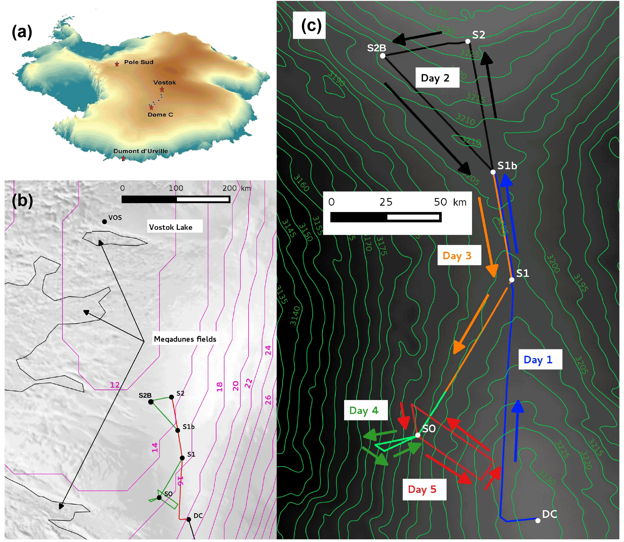
Figure 1Map of the route followed by the 2011/12 TASTE-IDEA traverse over the East Antarctic Plateau between the Dome Concordia (DC) and Vostok stations. (a) Locations of departure and destination base stations on the plateau. (b) The portion of the traverse along which radar profiles have been acquired. (c) Zoom detailing the 5 days of GPR profiling as well as the drilling sites of DC plus the locations of the firn cores retrieved during the traverse (S1, S2, S2B, S0) and used for dating the isochrones and deriving density profiles (see Sects. 3 and 4). The pink contours in (b) represent iso-values of the precipitation rate as computed by the ERA 40 model of the European Centre for Medium-Range Weather Forecasts (Simmons et al., 2007). Although the observed spatial and temporal variability is correctly reproduced, the precipitation is systematically underestimated (Genthon et al., 2015), and results require a systematic multiplying factor of about 1.5 to become realistic (Libois et al., 2014). Processes like sublimation and snow redistribution are omitted in the physics of the model and also explain the discrepancy with accumulation rate data.
In the present study, data acquisition is first described with the radar data summarized under a merged profile whose post-processing allowed the identification of three equally spaced IRHs covering the last 592 years. Special attention was paid to the vertical density distribution contained in the different ice cores of the project and used for computing the cumulative mass deposited above each of the three IRHs. Then follows a detailed error budget on the final computed accumulation rates which accounts for the three main sources of error stemming from the uncertainties in (i) density profiles, (ii) age and (iii) depth of the IRHs. Finally, spatial and temporal variations of the accumulation rates along the measured profile are discussed and compared (when possible) with results from previous studies.
2.1 Technical background and functional principle of GPR
The principle of GPR consists of measuring the two-way travel times of parts of an electromagnetic pulse emitted toward the ground that are reflected on discontinuities within the observed medium. When pulses are emitted at points along a profile, lateral continuity of the physico-chemical transitions within the medium yields wiggles of similar travel time (hence depth) along the resulting radar trace. Once put side by side, these wiggles are expressed in the form of horizons, also called IRHs, visible on the recorded radargram. In this respect, GPR is analogous to seismic reflection but with an electromagnetic wave instead of an acoustic wave.
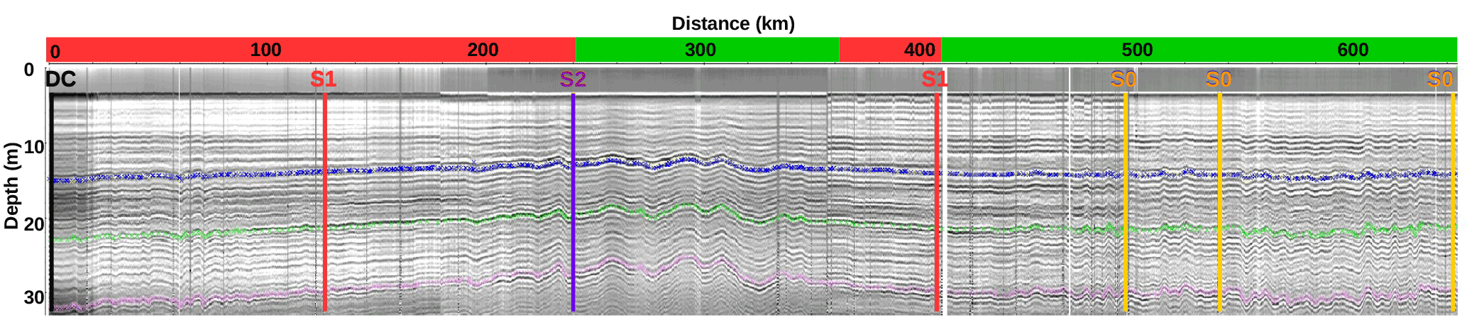
Figure 2Continuous post-processed radargram corresponding to the merged profiles as outlined in Fig. 1. The numerous observable IRHs result from as many reflections within the snowpack and are each characterized by a laterally varying depth and a specific age. The coloured (blue, green and pink) aligned dots emphasize the three most evident and continuous IRHs that are used in the present study. The radargram as depicted here (restricted to the first 35 m of firn) has undergone a time migration (see Sect. 2.3), meaning that the vertical axis represents true depths instead of two-way travel times. The apparently shifted vertical scale results from the time-zero correction. The horizontal axis is the cumulated distance along the profile as given by the GPS data. The white vertical stripe is due to a breakdown of the GPR leading to a gap of less than 2 km in the data. Also represented are the crossing points with the ice/firn cores DC, S1, S2 and S0 where the intersecting depths with the three selected IRHs have been inferred to check their isochronicity (see Sect. 4). The red and green upper banner refers to the position with respect to the topographic divide and correspond to the colour convention of the bottom right of Fig. 1 (red for “divide” and green for “off-divide” locations).
Discontinuities responsible for these partial reflections result in changes in the complex dielectric constant ϵ* of the medium. For the snowpack, essentially two main factors can be responsible for these changes as explained in Eisen et al. (2008) and references therein. The first concerns the real part, namely the permittivity, which varies with density, whereas the second acts on the imaginary part, which is sensitive to the conductivity of the medium. As a result, radar horizons within the first few hundred metres of firn and ice are essentially due to changes in density and acidity from volcanic deposits.
The huge advantage of the IRHs comes from their isochronous nature, although this has not been rigorously (physically) demonstrated, only heuristically by connecting ice core chemistry analysis of different drill sites (Eisen et al., 2004; Frezzotti et al., 2005) or by comparing accumulation rates obtained from both IRH depths and stake lines (Vaughan et al., 2004). This isochronicity is however understandable as it results from processes operating at the surface at the same time, such as acidic atmospheric deposits or density changes from the metamorphism of snow (at least the one initiated by surface interaction with the atmosphere like radiation crusts and wind redistribution). However, the physical processes leading to these IRHs still remain poorly known. For instance, as pointed out by Eisen et al. (2008), annual layers are still visible with radar wavelengths much larger than the annual thickness (a typical 100 MHz wave in the cold dry snow of the plateau has a wavelength of 2 m: much larger than the 10 cm annual snow thickness at Dome Concordia (DC) for instance), which contradicts the theory unless constructive interferences are considered as suggested by Palli et al. (2002) for instance.
Assuming isochronicity, the spatial variations of snow accumulation can be obtained from the varying depth of the IRHs. It thus implies transforming the two-way travel times of the reflected waves into actual depths. This is only possible if the wave velocity within the medium is known all the way from the surface down to the specific IRH and the time radargram is properly migrated (see Sect. 2.3). Inferring accumulation rates then requires the association of an age to the IRHs from independent means such as correct recognition of fallouts from identified volcanic and/or bomb testing events along firn/ice cores for instance (see Sect. 4).
2.2 GPR set-up
For the present project, GPR data were acquired with a MALÅ® ProEx GPR equipment fitted with a 100 MHz “rough-terrain antenna” towed behind one of the tractors used during the traverse with a constant separation of 2.2 m between the emitter and receiver parts. The apparatus, operating frequency and set-up are very similar to those used on a similar traverse between base stations of Dumont d'Urville and DC during the 2008/2009 austral summer (Verfaillie et al., 2012). The triggering was set to 1 s, meaning a radar trace every 4 m or so given an average speed of 14 km h−1 for the convoy. The time window was set to 1 µs (allowing for an investigation depth of some 100 m) and was sampled at 1.1 MHz, leading to roughly 1100 samples per trace. During acquisition a first improvement of the signal-to-noise ratio was obtained by an up to 64-fold stacking (which, given the time window of 1 µs, remained compatible with acquisitions made every second). Moreover, the system was connected to a GPS receiver mounted on the vehicle that recorded the geographic position of every single trace along the profiles.
2.3 Resulting GPR radargrams
Profiles outlined in Fig. 1 represent 5 days of measurements between 13 and 17 January 2012 and led to an almost continuous record of 630 km. The corresponding post-processed and concatenated radargram is shown in Fig. 2. The post-processing sequence consisted of time-zero corrections, a zero-phase low-cut filter (devow) to remove direct continuous currents and an “energy decay” gain to compensate for the volumetric spreading signal attenuation. Band pass filtering was reduced to a low-pass filter in the form of a spatial averaging over 50 traces which, given the huge number of traces (164 000 altogether), appeared more efficient than traditional finite impulse response (FIR) filters. Time-to-depth conversion was obtained by migrating the radargrams with the help of a vertical velocity profile for the radar wave. By investigating a similar region with similar firn properties, we followed the approach of Verfaillie et al. (2012), which consisted of only considering the effect of the firn density on the electromagnetic wave velocity as a result of dry and clean snow over the Antarctic Plateau. From the empirical relation of Kovacs et al. (1995) relating permittivity and density, the wave velocity c is obtained according to
with cv being the wave velocity in vacuum and ρ the firn density (relative to water density). The density profile comes from a recent core drilled at DC (Leduc-Leballeur et al., 2015) where high-resolution measurements allowed for a detailed profile (see Sect. 5.2). The true restitution of dipping reflectors theoretically requires a topographic migration, but the latter appears only necessary where the topographic variations are of the same order as the reflector depths. Given the extreme flatness of the investigated area of less than 2 m km−1 (topography of the upper surface and hence that of the IRHs), no such correction has been applied here. Last, ice sheet dynamics potentially changing the geometry of the IRHs has to be accounted for, except in the upper part of the ice/firn column, especially over areas of slow motion such as over the Antarctic Plateau as in the present case (Eisen et al., 2008).
The 102 m deep VOLSOL-1 ice core (VOLSOL programme; Gautier et al., 2016) is here used to time calibrate the IRHs observed with ground-penetrating radar. Owing to less reliable time–depth relationships, the three shallow ice cores (S0, S1 and S2, around 20 m deep each) retrieved along the TASTE-IDEA traverse will only serve as crossover points for assessing estimates of the age dispersion (see Appendix C). Details of sample preparation and analysis are presented in Appendix A.
3.1 Identification of volcanic eruption signals and volcanic chronology
Although sulfate in Antarctic snow comes from sea-salt spray and to a lesser degree from crustal erosion (Cole-Dai et al., 2000; Maupetit and Delmas, 1992), and principally from atmospheric oxidation of biogenic dimethylsulfide (DMS) emitted by oceanic phytoplanktonic activity (Prospero et al., 1991; Saltzman, 1995), volcanic eruptions are also major sources of during active eruptions. To identify volcanic signals in ice cores, it is thus necessary to calculate the non-sea-salt sulfate, (nss) corresponding to total sulfate minus sea-salt sulfate, and set a threshold above which spikes can be attributed to volcanic deposition. Over the East Antarctic Plateau areas, part of the sulfate background that could be related to continuous emissions from non-explosive volcanic activity seems to be minor (Castellano et al., 2004; Cole-Dai et al., 2000; Patris et al., 2000). The sea-salt sulfate contribution to total sulfate budget, evaluated using Na+ as a specific marker (Palmer et al., 2001; Röthlisberger, 2002), is less than 10 %. The Holocene crustal contribution, calculated by non-sea-salt Ca2+ as a continental dust marker (Castellano et al., 2004; Plummer et al., 2012; Röthlisberger, 2002), is even lower (< 0.05 %). Since these contributions are of the same order of measurement reproducibility, we did not correct sulfate concentrations and will not distinguish between total sulfate and non-sea-salt sulfate in the following discussion. However, particular attention was paid to developing a reliable method for distinguishing volcanic signals from non-volcanic sulfate background, and an outline of the method used is described in Cole-Dai et al. (1997, 2000), Stenni (2002), Castellano et al. (2004) and Igarashi et al. (2011). The procedure employed to identify candidate signals of volcanic eruptions in the sulfate profiles of the different cores follows that of Gautier et al. (2016).
Between five and eight volcanic events were identified in each TASTE-IDEA firn core, and 10 events were detected in the VOLSOL-1 ice core from the surface to 20 and 30 m through the application of the above-described procedures (see summary in Table 1). In the considered depths for shallow TASTE-IDEA cores and the VOLSOL-1 ice core, the main volcanic events in the 1601–2012 CE period are Pinatubo (Philippines, 1992 CE), Agung (Indonesia, 1964 CE), Krakatau (Indonesia, 1885 CE), Coseguina (Nicaragua, 1836 CE), Tambora (Indonesia, 1816 CE), unknown (1809 CE), Jorullo-Taal (Philippines, 1758 CE), Serua (Indonesia, 1695 CE), Gomkonora (Indonesia, 1676 CE) and Huyanaputina (Peru, 1601 CE). The sulfate deposition of the Kuwae eruption (Vanuatu, 1457–1458 CE; Salzer and Hughes, 2007; Sigl et al., 2013, 2014, 2015) can now be dated as 1459 CE, i.e. 5 to 6 years later than previously assumed (Gao et al., 2006, 2008).
Table 1Depths of the dating events along the mentioned cores from known volcanoes as well as thermonuclear bomb testing.
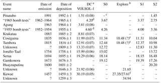
a The value in parentheses represents the depth shift to apply as the core was extracted a year earlier than radar measurements (see Sect. 4.2). b Time markers of the S0 and Explore cores have been merged to produce a hybrid depth relationship (see Appendix C). c A hyphen indicates an undetected volcano or an unmeasured nuclear fallout. d These two bomb test fallouts were actually measured on a nearby shallow core close to the VOLSOL-1 one in 2011/12 and served in the determination of its age–depth relationship. e Not accounted for in the resulting age curve since it was not clear to which volcano this sulfate peak should be attributed. f These two peaks, dated 1453 and 1460 CE, have recently been measured in the Explore core and are attributed to the Kuwae volcano (Robert Mulvaney, personal communication, 2017).
The temporal duration of volcanic signals in the ice has been evaluated by several studies (Castellano et al., 2004; Cole-Dai et al., 2000; Palmer et al., 2001), and general temporal durations range from 1 to 3 years. In this work, the temporal duration of volcanic signals lagged between 1.2 (3 consecutive samples) and 6 years (15 consecutive samples).
3.2 Artificial radionuclides deposition over Antarctica and associated chronology
Artificial radioisotopes resulting from atmospheric thermonuclear tests carried out between 1953 and 1980 were deposited in Antarctica after transport in the upper atmosphere and stratosphere, creating distinct radioactive reference levels in the snow. The dates of arrival and deposition in this polar region are well known and therefore provide a means to estimate Antarctic snow accumulation rates or describe air mass circulation patterns (Magand, 2009; Pourchet et al., 2003, and references therein). The 1955 and 1965 CE radioactivity peaks provide two very convenient horizons for dating snow and firn layers and thus measuring accumulation. Special techniques have been developed over the last 40 years to detect and measure artificial and natural radionuclides present in the ice sheets (Magand, 2009; Pourchet et al., 2003, and references therein). In Antarctica, 90Sr, 241Pu (deduced from 241Am analysis) and 137Cs radionuclides constitute the well-known debris products of atmospheric thermonuclear tests between 1953 and 1980 CE that we could still use to identify the two well-known reference layers in snow (1955 and 1965 CE peaks), corresponding to the arrival and deposition of artificial radionuclides in this region. Total beta counting and gamma spectrometry remain the most frequent radioactivity measurement device systems used to clearly detect artificial radionuclides and unambiguously determine the 1955 and 1965 CE peaks depths in the cores. The 1955±1 and 1965±1 CE peaks were both identified in each TASTE-IDEA firn core and in an extra-shallow core close to the VOLSOL-1 one (see Table 1).
4.1 Identification of major IRHs
Interpretation of radar data first consisted of identifying contrasting IRHs whose continuity could be tracked all along the entire merged profile. Three equally spaced IRHs were selected within the first 35 m of firn (no sufficiently clear reflectors could be used any deeper) and are emphasized with associated colours in Fig. 2. In order to properly capture the spatial variability, selection of these reflectors was done every kilometre or so, yielding each time a depth and the corresponding geographical position depicted as a coloured dot in the figure (the resulting number of dots leading to an almost continuous horizon). Of interest is the phasing of these three IRHs, which is characteristic of a stationary accumulation spatial pattern. It comes from the fact that local extrema in accumulation keep the same positions through time, allowing for cumulative effects with time which amplify IRH undulations with depth (Verfaillie et al., 2012).
4.2 Methodology for dating the IRHs
Dating is achieved by detecting the depths at which the reflectors intercept (or pass very close to) an ice/firn core where a depth–age relationship has been obtained (see Sect. 3). In the present case, as can be seen from Figs. 1 and 2, each of the three reflectors passes over several ice core locations and sometimes several times over the same one, thereby offering redundant dating possibilities. Due to its reliable dating curve including time–depth markers regularly spaced down to about 30 m, the DC-VOLSOL-1 core was selected as the reference and served for proposing an age ab initio for each of the three IRHs. The choice for the DC core is also justified by the numerous available ice core dating schemes for the site which gives a good level of confidence in the proposed age–depth relationships (Parrenin et al., 2007).
As for the other cores of the project, the dating is less reliable as the result of shallower depths, making the resulting fits questionable for the 2 deepest IRHs. A longer record has been artificially derived from the shallow S0 core supplemented by the nearby (70 m) 110 m deep Explore core from the companion Explore programme. Because of ambiguity with a sulfate peak at 10.48 m, only the very deepest points of the Explore core have been used to supplement the S0 age–depth relationship (see Fig. C1) used for estimating the age dispersion as described in Appendix C.
Having been extracted during the VOLSOL programme (2010/2011 field season), the DC-VOLSOL-1 core is a year older than the radar measurements. As a consequence, a depth correction has been applied to each IRH volcanic depth in the form of a downward shift of 8 cm (modern snow-equivalent accumulation for DC) weighted by the density ratio between the relevant depth and the surface (i.e. 8 cm for the surface, reducing to 4.53 cm for the Kuwae volcano at the depth of 31.20 m; see Table 1).
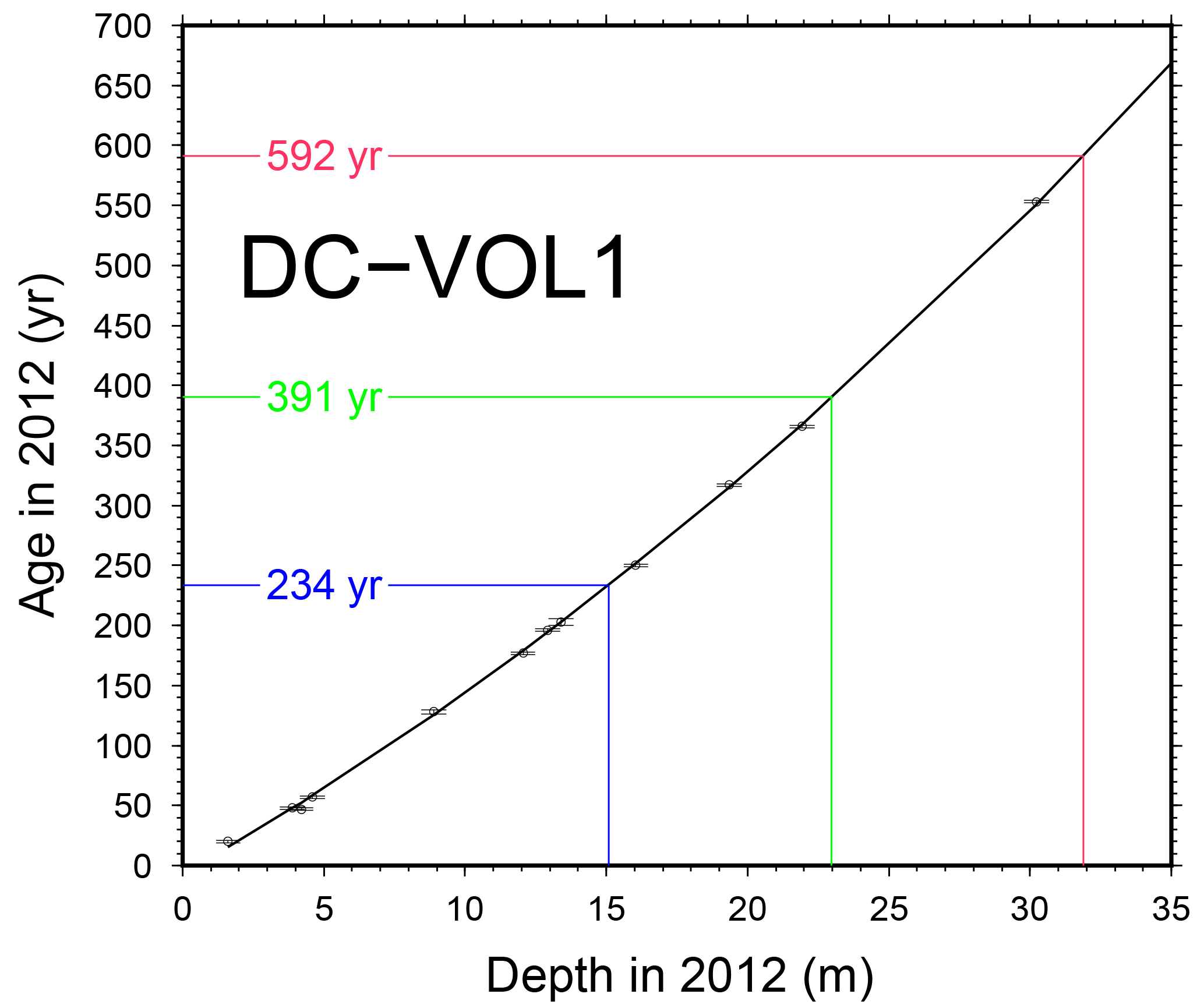
Figure 3Identified and dated deposits placed in an age–depth representation according to their depths within the DC-VOLSOL-1 ice core. Volcanic horizons were completed here by the integration of the two 1955 and 1965 thermonuclear horizons (depths of 4.20 and 4.60 m) from dedicated measurements along an extra core drilled at DC in 2012 during the scientific traverse. A degree-2 polynomial fit (black line, r2>0.99) was then used as a continuous dating curve permitting the dating of any intermediary depth.
4.3 Age results and the isochronous character of the IRHs
As can be seen from Fig. 3, IRH depths of 15.08, 22.97 and 31.89 m at the VOLSOL-1 core location respectively give ages of 233.74, 390.54 and 591.71 years (later rounded to 234, 391 and 592 years).
The two main factors that can potentially alter the isochronous character of the selected IRHs are (i) errors in age–depth relationship at each coring site and (ii) errors in the depth estimates of the IRHs at these same sites deduced from the radargrams. As for the first, owing to the short-scale changes in snow deposition and erosion as expressed by the surface roughness, the archiving process can sometimes be significantly different for neighbouring cores, thereby raising the problem of the correct representativeness of a single core. For several volcanoes Gautier et al. (2016) found differences in the depths of the corresponding sulfate peaks by as much as ±20 cm from one core to the other among a set of five different cores all separated by 1 m. As a consequence, on top of errors in the correct depth measurements of the chemical peaks, surface processes lead to an uncertainty in the core-derived age–depth relationships. Figure B1 in Appendix B reports the time markers along the five cores from the study of Gautier et al. (2016). From quadratic fits along each core, five different ages are computed for our IRH depths of 15.08, 22.97 and 31.89 m, yielding respective root mean square (rms) deviations of 6, 7 and 7 years with respect to our reference ages of 234, 391 and 592 years. These deviations can be considered as good estimates of the uncertainty in the correct representativeness of the single core of our study. The residency time of volcanic aerosols in the stratosphere (from 2 to 4 years) is variable from one volcanic event to the other and therefore also contributes to some uncertainty in the depth–age relationship, which makes for an overall uncertainty of 8 years in the age for a given depth, a result very similar to that of Eisen et al. (2004).
As for the depth accuracy of the selected IRHs, it mainly results from the physics of radar and the chosen frequency for the electromagnetic wave. Eisen et al. (2004) gives a review of all possible resultant sources of errors, and their results are applicable to our case because of the use of the same commercial radar set from MALÅ® Geoscience Sweden, with the only difference being that they use 200 and 250 MHz frequencies instead of our 100 MHz. One initial source of uncertainty lies in the thickness the 100 MHz wave can resolve. Although it theoretically amounts to λ∕4, one-fourth of the wavelength in the firn, λ∕2 is usually considered as more realistic, which in our present case gives 1 m. Additionally, the pulse width also matters (length of the energetic part of the source wavelet) and was determined by common midpoint analysis to be 12 ns with our system (Verfaillie et al., 2012), leading to a tracking accuracy of half this duration, which in the firn gives a shift of some 1.2 m. Since these two errors do not systematically add up, one generally considers the worse of the two. Finally, interpreting radargrams and picking reflectors are partly subjective and operator-dependent processes, which leads us to estimate the overall uncertainty of the IRH depth to be 1.5 m at the worst. Given a relatively constant slope of 20 yr m−1 of the age–depth relationships (see Fig. 3), this depth uncertainty maps into an age uncertainty of about 30 years. This uncertainty in the depth positioning nevertheless has a strong systematic component (in other words the error in depth positioning remains mainly the same along a given IRH) and therefore only partly alters the isochronous character of the reflectors. The same can be said for depth errors resulting from a wrong assessment of the vertical velocity profile. Only lateral variations not properly accounted for would contribute, but it is well known that the plateau firn only undergoes minor lateral variations in its depth distribution of density (Muller et al., 2010) and hence velocity at the scale of a couple of hundred kilometres. As a result, one can reasonably argue that a true isochronous IRH can theoretically deviate by 10 to 15 years. Appendix C presents the different inferred ages when reporting our IRH depths along the other cores of the project (S1, S2 and S0–Explore). From the rms dispersions of respectively 3, 6 and 13 years for IRHs 1, 2 and 3 at the crossover points as revealed by Fig. C1 we come to the conclusion that our three IRHs can be considered as isochronous. We nevertheless have to keep in mind that the absolute error of the age (to be used in the budget error for mass balance computation; see Sect. 5.6) remains potentially higher than these 10 to 15 years by integrating the biases from systematic incorrect positioning and errors from time-to-depth conversion in the radargrams.
5.1 Accumulation computation
Assuming an IRH at a given depth H, the total mass M of the unit surface (1 m by 1 m) firn column above it can be expressed as
where M can be considered as a mass flux per square metre because of the implicit unit surface. It is therefore expressed in units of kilograms per square meter which, given the density of water, also represents millimetre water equivalent. The average accumulation rate over the period since the deposition of the IRH is finally obtained by dividing by the age of the IRH, leading to a final result in millimetre water equivalent per year.
5.2 Firn density profiles for accumulation rate computations
Similarly to the depth and age, proper estimation of the density profile down to a given IRH is crucial for a good assessment of the corresponding accumulation rate. If spatial variations of accumulation mainly result from differences in snow cumulative heights as revealed by undulating reflectors, one can reasonably wonder to what extent geographical changes in density may also have an impact. Unfortunately, over the Antarctic Plateau, density profiles are usually concentrated at limited sites with almost no reliable data in between. In the present case, density profiles from deep ice cores are only available at the two “extremities” of the radar line (DC and S0). Some extra-shallow cores were also drilled along the radar profile (S1, S2, S2B) but their maximum depths (about 20 m) are limiting at least for interpreting the two deepest IRHs. However, owing to the fact that over the plateau meteorological parameters controlling the densification process (e.g. air temperature, wind activity, solar radiation) exhibit small gradients at the regional scale, a relative uniformity in firn density profiles can be first assumed over distances of the order of 100 km as can be anticipated from the small divergence between the DC and S0 density profiles (see Fig. 4). The limited variability was confirmed by Fujita et al. (2011) from pits and surface snow measurements during the JASE traverse, and more specifically the resulting small impact on accumulation rates was demonstrated by Ruth et al. (2007) when comparing water equivalent depth profiles between Dome Fuji and EPICA (European Project for Ice Coring in Antarctica) DML (Dronning Maud Land). This led us in a first instance to consider only deep ice cores from the DC site along which precise and high-resolution density profiles have been performed (Leduc-Leballeur et al., 2015). A later sensitivity test is proposed (see Sect. 5.4) consisting of assessing changes in accumulation to expect from integrating the contribution of density profiles from different locations. These changes would then be compared to the uncertainties solely arising from the degree of representativeness (due to the small-scale variability) and measurements errors in density when using a single density depth profile for computing the accumulation rate all along the radar line (see Sect. 5.5).

Figure 4Density profiles (left scale) as mentioned in the text and detailed in Table 2. Also shown in the bottom part is the corresponding cumulative mass with depth (right scale). For the sake of clarity, only cores (and associated cumulative masses) exceeding 20 m are fully represented (DC5, DC3, Firetracc and ITASE-98 ice cores). Insets correspond to enlargements around the depths of IRHs 1, 2 and 3 where all mass curves are depicted and allow for an estimation of the dispersion in cumulative masses and in the resulting accumulation rates (to be used later in Sect. 5.5). The upper panel shows a comparison of the DC5 and S0 (Explore) density profiles with estimated measurement error bars that only served for the computation of the uncertainty in the wave velocity profile (see Table 3).
Table 2Density cores at DC along with the characteristics of their quadratic fits. Cumulative masses (kg m−2) down to each of the three IRHs at respective depths of 15.08, 22.97 and 31.88 m are computed from the raw data as well as from the fitted curves.
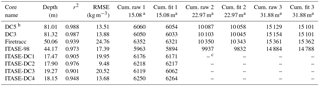
a In kg m−2. b Leduc-Leballeur et al. (2015). c Depth not reached by the core.
5.3 Density profiles at DC
In the framework of the EPICA project (Augustin et al., 2004), along with the main core, several extra-shallow drilling projects have yielded as many density profiles over at least the first 50 m for the DC area (see Table 2 and Fig. 4). A first question arises as to which of these cores to use for computing accumulation rates; in other words, what can be the sensitivity of the results to the choice between different nearby cores at a given site like DC? The lower part of Fig. 4 shows the depth–density profiles for each of the cores listed in the table along with the corresponding cumulative mass with depth (right scale in the figure). The cumulative masses have been computed either from the raw data or from the quadratic fits (see corresponding results at the three IRH depths in the table). Despite a pronounced scatter in the individual data points around their respective fits (see Fig. 4 and associated root mean square error (RMSE) in the table), considering raw or fitted data does not significantly change the depth–cumulative mass with differences not exceeding 1.15 % at the most (ITASE-98 at the depth of IRH1). This illustrates a random scatter of data points above and below the fit, which leads to an almost exact compensation when summing up the cumulative mass. As a consequence, fitted density curves will hereafter be considered in the computations of accumulation rates. The second result comes from the limited dispersion in the cumulative mass from one core to the other as can be easily seen from the figure. The maximum discrepancy is to be found between the ITASE-98 and Firetracc ice cores with relative differences of 7, 5 and 4 % at the depths of respectively IRHs 1, 2 and 3. Of interest is the almost perfect overlap of the DC3 and DC5 curves, which come from the same project and have been measured according to the same protocol by the same operator. These results tend to show the following:
- a.
Most of the difference between different cores results from measurement errors.
- b.
The variability of the density expressed at the scale of the typical distance between these cores (from metre to kilometre scale) is of stochastic type (Libois et al., 2014) and is therefore rapidly cancelled out by the depth-averaging process of cumulative mass computation leading to accumulation rates. Indeed the DC3 and DC5 cores are separated by 1.5 km but still show remarkable consistency in their quadratic fits or in their associated cumulative mass distribution with depth.
- c.
Provided that systematic error measurements can be minimized, a single density profile should be considered as representative of the local accumulation rate.
The very good similarity of the DC3 and DC5 cores attests to the quality of density measurements as confirmed by the novelty and strictness in the measurement protocols (Leduc-Leballeur et al., 2015). This led us to choose the DC5 as the reference for our accumulation rate computations.
5.4 Sensitivity of the accumulation rate to geographically different density profiles
Figure 5 shows the three accumulation rates derived along each of the three IRHs along the radar line from the density profile provided by the DC-5 reference core. Since the computation uses a single density profile, no lateral changes in density are accounted for, and the stationary accumulation pattern is therefore expressed as shifted IRHs of the same shape. Of importance is the pronounced gradient when following the ridge going from DC towards S2 (see map in Fig. 1) with a more than 20 % loss within 250 km.
In order to test the sensitivity to the use of density profiles originating from different distant places, accumulation rates are separately computed here from both the reference DC5 density profile and the Explore one (the latter being the only reliable and deep enough density profile at our disposal). The difference is expressed in the form of a uniform shift along a given IRH (as can be seen from the insets) but with a decreasing sensitivity with the depth of the IRH. The difference in accumulation rates from the use of the DC and S0 (Explore) densities amounts to 1 mm w.e. yr−1 for the 234-year IRH1 (lower inset) and reduces to about half of it when considering the 592-year reflector (upper inset). The explanation is to be found in the rapidly converging fits of the DC and S0 density curves with depth (top of Fig. 4). Indeed, the increasing cumulative difference in mass is more than counterbalanced when dividing by the age of the IRH in the accumulation rate computation process. Using the less reliable S1, S2 and S2B (not represented) did not lead to a significantly higher sensitivity. As a consequence, a maximum deviation of the order of 1 mm w.e. yr−1 is to be expected from accounting for the geographical changes in density along the profile.

Figure 5Computed accumulation rates since the deposition of the three IRHs according to the polynomial fit of the DC-5 density profile. The lower inset represents an enlargement over the dotted square and shows the sensitivity of the accumulation rate at the uppermost IRH to the use of the DC-5 and S0 (Explore) cores, whereas the upper one does the same but for the lowermost IRH. Error bars represent the estimated uncertainty resulting from the combined density error measurements and small-scale spatial variations. These error bars (see Sect. 5.5) are only depicted once since they are uniform all along the profile. Ranges for the accumulation rate at S2 inferred from the SR50 sensor (see Sect. 6.1) are represented by the black box along the S2 vertical line.
Table 3Different source terms in the overall error budget for accumulation rate.
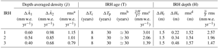
a rms of and . b rms of ΔTc and ΔTp. c Computed with averaged depths of respectively 13.87, 21.09 and 29.43 m and corresponding averaged densities of respectively 397, 498 and 553 kg m−3 for IRHs 1, 2 and 3. d rms of ΔHr and ΔHv.
5.5 Proper choice of the density core to use
Assessing the uncertainty in the accumulation rates solely arising from measurement errors in the density profile used is not straightforward since some of these errors are random and certainly compensate with depth, a least partially. Moreover, small-scale accumulation variability that influences the representativeness of a single core for a given location also potentially contributes to accumulation uncertainty, even if limited in amplitude as was shown in Sect. 5.3. Because they result from different projects, implying different measurements protocols, the numerous cores drilled in the DC area provide a means of estimating the order of magnitude of the combined effect of these two terms. In particular, the dispersion between all these cores should implicitly include most of the measurement errors and would only miss a systematic component (i.e. an identical error for all measurements), which in any case must remain small. Computation of the cumulative mass down to IRH1 for these eight cores listed in Table 2 gives an average of 6127 kg m−3 with a standard deviation of 141 kg m−3. When dividing by the age of IRH1 (234 years), one obtains 26.18±0.60 kg m−3 yr−1 or 26.18±0.60 mm w.e. yr−1. Similar computations down to the two deepest IRHs (but only concerning the first four cores) respectively give 25.75±0.54 and 25.49±0.40 mm w.e. yr−1 for IRHs 2 and 3.
The resulting dispersion is then considered as representative of the total error due to the use of a local density curve and has been represented in the form of the error bars in the insets of Fig. 5. The same error bars have been applied to the accumulation profiles from the Explore core at S0, but they probably represent an underestimation due to a less stringent density protocol in the density measurement. From the systematic overlap and the fact that the Explore error bars represent lower bounds, we come to the conclusion that accounting for the available geographical spatial variability of density does not cause significant changes in the accumulation rates. In fact, properly accounting for the geographical distribution of density would normally require integration of all available density profiles evenly distributed along the radar line according to their respective distances (inverse distance weighting). However, the S1, S2 and S2B cores are of limited use because of a maximum depth of 20 m. Moreover, including the effects of density at S0 (potentially different from that at DC) according to an inverse distance weighting would not make much sense when considering the position of the S0 profile with respect to the entire radar profile (the DC–S0 gradient being perpendicular to the major axis of the radar line; see Fig. 1). As a consequence, our strategy thus consists in relying on a single but reliable density profile (DC5) rather than trying to integrate the non-significant geographical effects from limited or not-so-relevant extra data sets.
5.6 Overall error budget for surface accumulation rates
From the expression of snow accumulation rate , the three error sources contributing to the overall uncertainty originate from (i) ΔH, the error in the depth of the IRH; (ii) ΔT, the error in its age; and finally (iii) , the density error resulting from the use of the selected density profile. All the resulting components are summarized in Table 3. The first error term () due to density implicitly includes the uncertainty resulting from the degree of representativeness and the measurements errors of the selected core (DC5). It has already been assessed from the dispersion in accumulation rates of the numerous available density profiles at DC (see Sect. 5.5) and is directly expressed as an accumulation rate uncertainty (0.6, 0.54 and 0.4 mm w.e. yr−1 for respectively IRHs 1, 2 and 3). As for the error due to the neglect of the geographical changes (), it can be estimated to be around the average along the radar line of the difference in accumulation rate when using the DC5 and the S0 core (Sect. 5.4), namely 0.98, 0.85 and 0.68 mm w.e. yr−1 for respectively IRHs 1, 2 and 3. The overall error due to density is finally proposed as the rms of these two terms (see Table 3).
For the age, the two independent terms arising from (i) the relevance and associated uncertainty of the age–depth relationship of the used core ΔTc (8 years) and from (ii) the positioning error due to radar resolution ΔTp (30 years; see Sect. 4.3) give a quasi-systematic rms remaining around 30 years. This time error thus transforms into accumulation rate uncertainties of respectively 3.01, 2.06 and 1.39 mm w.e. yr−1 for IRHs 1, 2 and 3.
Finally, errors in the depth (H) of the IRHs stem from the 1.5 m radar positioning accuracy as determined in Sect. 4.3 plus a systematic component due to the time–depth conversion of the two-way travel time. Proper derivation of Eq. (1), with an average error of 18 kg m−3 in density measurements (deduced from the estimated density measurement errors represented by the error bars of the DC5 density profile in Fig. 4), gives a relative error of less than 1.5 % for the average wave velocity. It leads to the resulting depth error ΔHv as a function of the IRH depth as given by Table 3. The rms combination of these two terms finally gives an error component for the accumulation rate of respectively 2.54, 1.68 and 1.23 mm w.e. yr−1 for IRHs 1, 2 and 3.
Following Muller et al. (2010), the cumulative uncertainty is finally proposed as the rms of these three main contributors (, ΔT and ΔH), which gives global maximum uncertainties of 4.12, 3.02 and 2.17 mm w.e. yr−1 for IRHs 1, 2 and 3 respectively, later rounded to 4, 3 and 2 mm w.e. yr−1. The noticeable feature is a strong decrease with IRH depth, in contrast to Muller et al. (2010), where an increasing error with depth seems to result from a rapid degradation of the signal-to-noise ratio due to the weak penetration depth and high sensitivity to water content of their high-frequency (2.3 GHz) system. It should also be noticed that the proposed uncertainties here pertain to the absolute errors in the accumulation rates and implicitly comprise a significant systematic part that does not come into play when interpreting spatial or time-dependent gradients as in the following section.
6.1 Spatial distribution
A geographical representation of averaged accumulation rates (and differences between the fields) over the three periods characteristic of the three selected IRHs is represented in Fig. 6, where significant trends can be observed. The relatively good phasing between the three IRHs already noticed on the radargram is observable from the difference in the represented fields (blue scale) not exceeding 1.2 mm w.e. yr−1. It is also consistent with the computed SMB of Fig. 5 and confirms a quasi-stationary accumulation pattern over the past 600 years. In particular, an overall decrease in accumulation of some 20 % from DC to the south-west (towards S2) similarly appears for the three IRHs. More specifically, traversing towards the south-east leads to the minimum value between 19 and 20 mm w.e. yr−1 (depending on the averaging period) at a place close to the S2B core site in the direction of a nearby megadune field (see Fig. 1).
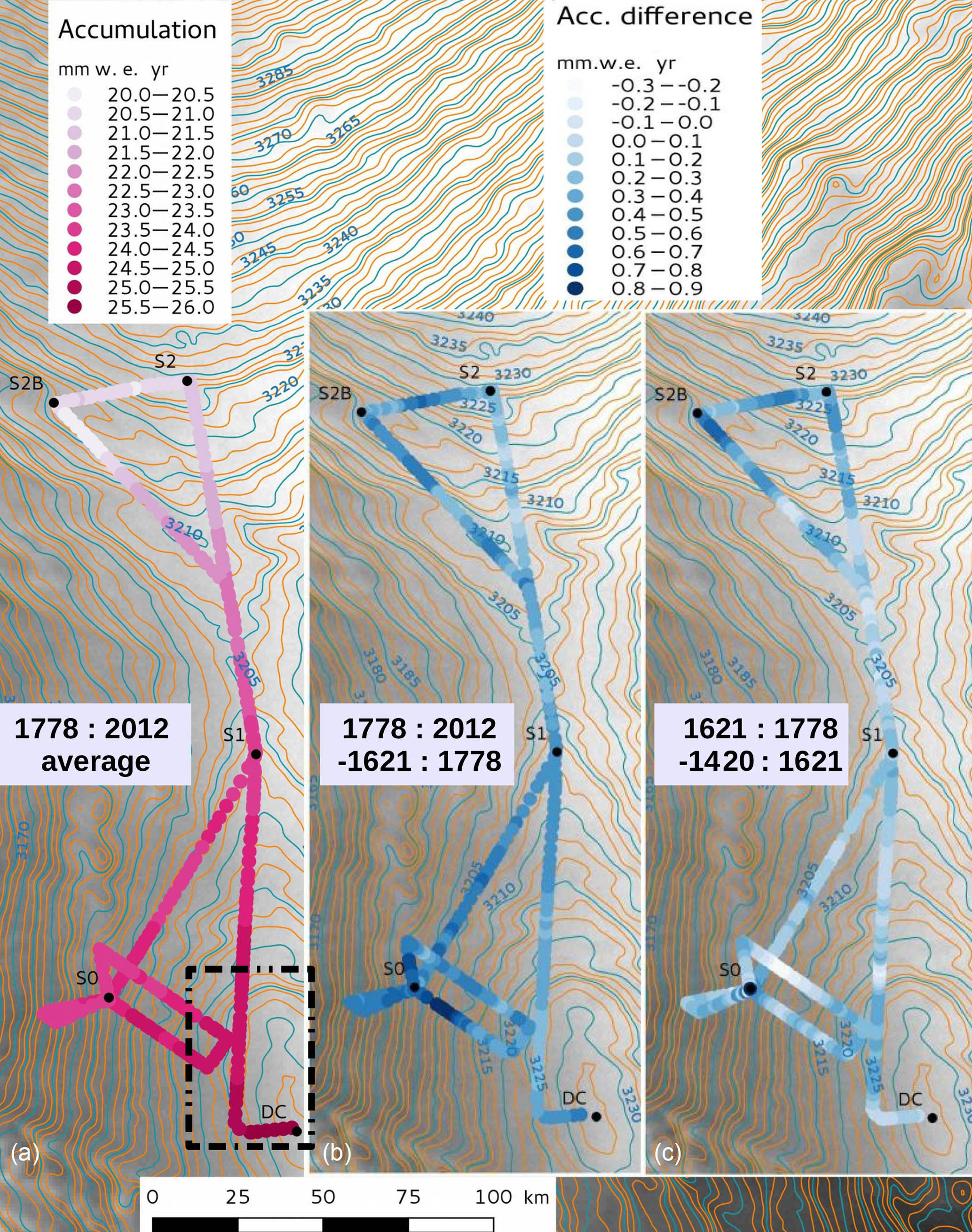
Figure 6Geographical (polar stereographic, 71∘ S) distribution of net accumulation rates according to the ages of the three IRHs. Panel (a) is the average over the last 234 years (1778–2012 CE), whereas panel (b) represents the latter field minus the 1621–1778 CE average. Last, panel (c) stands for the difference between the 1621–1778 and the 1420–1621 CE periods. Globally positive values in these differences confirm a steady overall increase through time as revealed by Fig. 9. Background is a RADARSAT image of the prospected area revealing some topographic features emphasized by the contour line of the surface digital elevation model (Bamber et al., 2009).
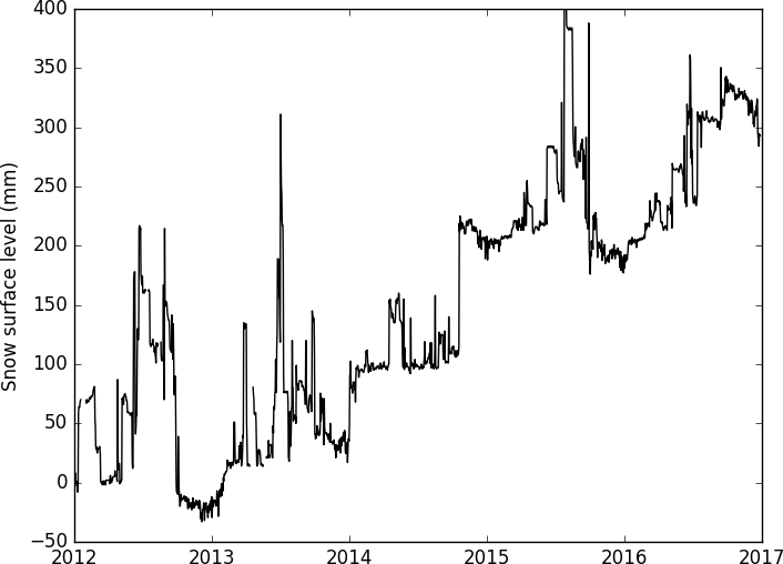
Figure 7Snow surface level in millimetres above the reference level of 1 January 2012 obtained from acoustic distance measurements. Presented daily mean values were calculated from measurements recorded every 30 min and corrected for air temperature.
It should be noted that the 2011/12 TASTE-IDEA traverse was the opportunity for the deployment of an ultrasonic range sensor (SR50, Campbell Scientific) allowing for a continuous monitoring of the surface height for more than 5 years at the S2 point. Corresponding surface heights since January 2012 are depicted in Fig. 7, where short-term variations revealing both precipitation and/or strong snow redistribution events are clearly visible. Despite these rapid changes, which eventually contribute to the metre-scale variability in surface accumulation (Libois et al., 2014), a significant trend emerges over these 5 years of measurements. When considering surface densities between 300 and 330 kg m−3 (Fig. 4), this trend maps into accumulation rates between 19.5 and 21.5 mm w.e. yr−1, which appear to be fully consistent with our computed accumulation rate for the S2 point over the last 234 years as represented by the black box in Fig. 5.
Previous measurements of GPR-derived accumulation rates in the vicinity of Concordia Station were carried out in 2005 (Urbini et al., 2008). A radar profile through the station revealed an almost north-to-south gradient of mm w.e. yr−1 km−1 in its southern part (see Fig. 6 in Urbini et al., 2008, and Fig. 8, where corresponding data have been summarized). Despite limited areas over which they overlap, and a slightly different averaging period (the last 266 years against our average of the last 234 years), these data nevertheless remain relatively consistent with ours as can be seen from the figure. Moreover, from our data, starting from around DC and considering the upper left blue points of the figure, a difference of about 1 mm w.e. yr−1 can be derived over a distance of some 30 km, leading to a gradient of −0.033 mm w.e. yr−1 km−1: close to that of Urbini et al. (2008) along a similar direction. When assessing an uncertainty in our proposed gradient, only the non-systematic terms have to be considered, such as the effects of a laterally varying density, which in the present case should be insignificant because of the distance of only 30 km. Errors in positioning or age along IRH1 should also remain small. Indeed, as can be seen from the limited dispersion in both ages and depths at crossing points S1 and S0 (see Table 2), the spatial variations in positioning or in the age along a given IRH are minor (maximum differences of 18 cm and 3 years for IRH1, leading to a rms uncertainty of 0.43 mm w.e. yr−1 according to the error budget of Table 3). It leads to an uncertainty of 0.014 mm w.e. yr−1 km−1 on the proposed gradient and makes the comparison still relevant.
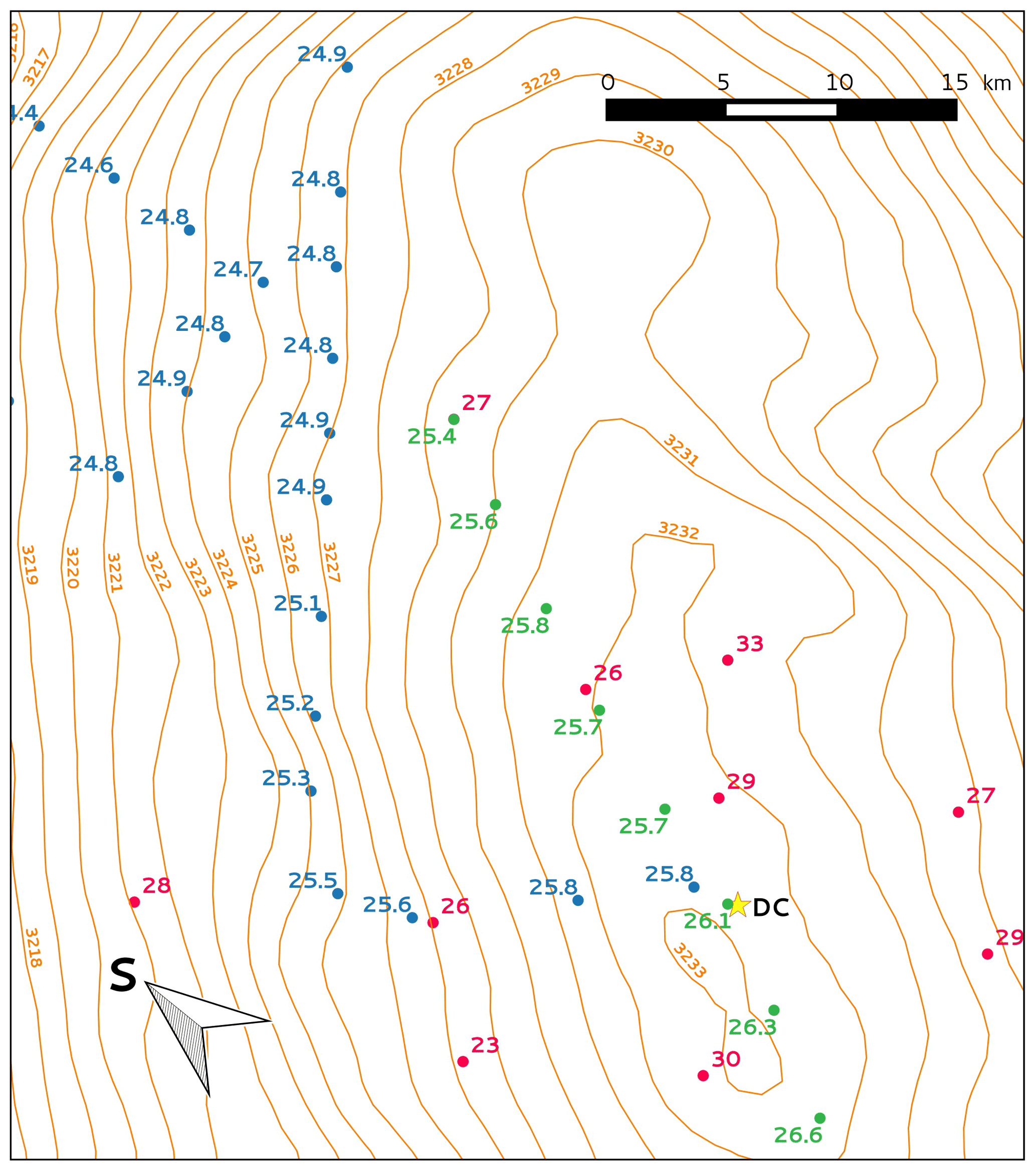
Figure 8Comparison of our accumulation rates with those in Urbini et al. (2008) in the vicinity of Concordia Station over the area featured by the dashed inset of Fig. 6. Blue dots represent the rates as represented in Fig. 6 for the last 234 years, whereas the green ones are those from the radar transect of Urbini et al. (2008) after being equally sampled (5 km) and averaged over five measuring points. Also shown by red dots are accumulation rates inferred from an analysis of firn cores based on tritium ∕ β markers for the 1965–2000 period (Urbini et al., 2008) and for which an uncertainty of 10 % has been derived. Contours are altitude above sea level as given by Bamber et al. (2009). The Concordia Station is featured with a yellow star.
It should be noted that this gradient has also been observed by Genthon et al. (2015) from snow accumulation at two stake networks 50 km apart along a north–south direction centred on the Concordia Station. Despite a high uncertainty for the uppermost snow density which limits the derivation of absolute values of accumulation rate, the use of a uniform snow density along the 50 km long section revealed a significant gradient similar to that of Urbini et al. (2008) and of the present study. Their study also shows that, despite an overall underestimation of snow accumulation, meteorological analyses from the European Centre for Medium-Range Weather Forecasts confirm this tendency (see the modelled precipitation field in Fig. 1). Moreover, from a careful observation of precipitation events and analysis of air mass back-trajectory pathways, Genthon et al. (2015) show that the core of snowfall results from relatively warm (and hence humid) air masses intrusions from the north. When passing over the Concordia dome on their way to the south, they undergo a significant temperature-driven depletion in moisture, which is fully consistent with the observed gradients.

Figure 9Time-dependent evolution of the accumulation rates spatially averaged over five sectors along the radar profile. The first sector corresponds to the DC vicinity (green squares on the map) within the firn core network as in Urbini et al. (2008) and featured by the red spots in Fig. 8. The second sector more or less follows the ridge from the end of the DC sector down to a topographic saddle (orange circles). The third (blue diamonds) continues along the ridge and climbs up to the S2 point. The fourth (purple stars) follows the perpendicular S2–S2B transect, whereas the fifth (brown triangles) comprises the vicinity of the S0 point. The time frames for the time averaging (a) correspond to the age difference from each of the three IRHs to the next above or to the surface, namely 1420–1621, 1621–1778 and 1778–2012 CE. Also presented with grey symbols are the accumulation rates as reported by Frezzotti et al. (2005) and Urbini et al. (2008) over the DC area (see text) and for which error bars of ±10 % occur (not shown for clarity). Surface topography with 2 m contours is that of Bamber et al. (2009).
6.2 Time dependency of accumulation
Because of the limited number of IRHs being analysed in this study, only a coarse characterization of the time-dependent accumulation can be proposed as is the case in Urbini et al. (2008) for instance. This limitation comes from the stringent requirements for a reflector to be considered as properly isochronous (showing continuity over large distances) and assigned a relevant age (by passing through a coring site where an depth–age relationship can be independently derived). As for recent accumulation rates, it should be noticed that the multiple direct reflections in the air between the emitter and receiver parts of the antenna lead to a saturated signal screening potential sub-surface reflectors. The last decades of surface mass balance from GPR are therefore often missing, which prevents proper comparisons with “modern” accumulation values as derived from stake farms for example (only operational since the late 1990s for the DC area).
We therefore propose three periods over which mean accumulation rates can be derived (1420–1621, 1621–1778 and 1778–2012 CE) as can be seen from Fig. 9. Data were spatially averaged over five main sectors whose respective extensions are reported in the figure with appropriate symbols. As for the associated uncertainties (depicted in the form of the proposed error bars in the figure), amongst the various terms of Table 3, only the non-systematic components have been kept. For instance error due to density is now restricted to the term since results from potentially unaccounted-for geographical changes in density. It leads to respective accumulation rate uncertainties of 0.6, 0.54 and 0.4 mm w.e. yr−1 for IRHs 1, 2 and 3 respectively. For the age uncertainty, we considered ΔTc (error of 8 years resulting from the age–depth relationship) and the effects of a reduced positioning uncertainty ΔTp of 0.5 m (since most of it is time-independent) leading to an age uncertainty of 10 years. Considering the average slope in the age–depth relationship, the global rms age error (13 years) maps into respective uncertainties of 1.3, 0.9 and 0.6 mm w.e. yr−1. Finally, for the error solely due to positioning and its effect on the cumulative mass, we restricted to the above-mentioned 0.5 m and neglected errors stemming from the uncertainty in the velocity profile. It thus leads to accumulation uncertainties of respectively 0.85, 0.64 and 0.47 mm w.e. yr−1 for IRHs 1, 2 and 3. The corresponding total errors finally result from the rms of these three terms yielding the ±1.66, ±1.23 and ±0.86 mm w.e. yr−1 error bars reported in the figure.
The figure shows an overall accumulation increase which appears consistent from one sector to the other. Such a uniform increase is in line with the stationary character in the spatial distribution as already observed in Figs. 5 and 6 for example. Our results compare well with those mentioned in Urbini et al. (2008) and references therein over the DC area (depicted in grey in the figure). More specifically, from nss volcanic spikes along the EPICA EDC96 core, an average accumulation rate of slightly less than 25 mm w.e. yr−1 for the 1460 (Kuwae)–1816 (Tambora) period was proposed (Castellano et al., 2004). Then follows the 1816–1998 AD period with a 25.3 mm w.e. yr−1 accumulation rate overlapped by a marked increase up to 28.3 mm w.e. yr−1 between 1965 and 2000 deduced from nuclear test horizons along the firn cores represented by the red circles in Fig. 8 (Frezzotti et al., 2005). Unfortunately, these last results also suffer uncertainties (estimated to be 10 % of their value), which casts some doubt on the reliability of possible deduced time trends.
Accumulation rates from stake farms are also proposed by Frezzotti et al. (2005) with 32 mm w.e. yr−1 for the 2004–2007 period and up to 39 mm w.e. yr−1 between 1996 and 1999, but their relevance is also questionable because (i) the measuring period is extremely short with respect to a very high interannual variability; (ii) the derived accumulation rate requires proper knowledge of the sub-surface density, which is highly variable and difficult to accurately measure; and (iii) the intrinsically strong spatial variability in snow thickness at the scale of a stake farm also requires long integration periods to gain in significance. This is confirmed by the associated standard deviation of 14 mm w.e. yr−1 for the 1996–1999 stake results. In any case, no comparison with radar data is possible because of corresponding reflectors too close to the upper surface to be detected. More generally, other studies along the East Antarctica Ice Divide (Dome C, Vostok and Dome Fuji) suggest similar increases of surface mass balance during the last century (Frezzotti et al., 2013; Fujita et al., 2011; Osipov et al., 2014; Urbini et al., 2008). If the results proposed here appear consistent with these studies, their associated uncertainties unfortunately remain too large (even after being diminished by the time-independent biases) to serve as incontrovertible evidence of a significant time increase in the accumulation rates.
Relative depths of three IRHs from a 630 km long GPR profile have been combined with time markers as well as density profiles along ice core data to provide surface accumulation estimates between the DC and Vostok stations on the Antarctic Plateau. Results show a remarkably persistent accumulation pattern, whatever the investigated time period (1420–1621, 1621–1778 and 1778–2012 CE). More specifically, over the last 600 years, the average accumulation rate exhibits a significant NE–SW gradient from 25±2 mm w.e. yr−1 at DC to 19±2 mm w.e. yr−1 at the other extremity of the profile, which appears to be consistent with previous radar data available in the vicinity of DC. As for the time dependency, despite an observable steady increase of about 3–4 % over the last 600 years which partially matches that from similar radar data, unbiased errors still prevent reliably inferring a positive time trend in accumulation. The careful error analysis that is proposed accounts for all possible intervening terms and provides depth-dependent maximum margins of error for the absolute accumulation values ranging from 2 mm w.e. yr−1 (592-year average) to 4 mm w.e. yr−1 (234-year average). It also shows that, despite the proven isochronous character of the proposed IRHs, the main source of error is to be found in the uncertainty in the determination of the IRH depth. Not only does this 1.5 m error change the depth over which the mass is accumulated, but it also leads to 30 years in the IRH age determination and eventually contributes to most of the total uncertainty in the accumulation rates. The error budget also shows that in our case the uncertainty in terms of density resulting from both the representativeness and measurement errors of a single core is of the same order as the changes expected from incorporating the potential geographical variability in density from extra (but less reliable) cores along the radar line. In other words, it proved better to exclusively rely on a single reliable and accurate density core at one extremity of the profile, rather than trying to incorporate doubtful spatial changes from less reliable or even non-exploitable intermediate density cores.
Measuring surface mass balance over Antarctica remains a challenge; amongst the different available methods, combined radar and ice core data provide a robust means of properly assessing large-scale spatial patterns and to a lesser degree long-term temporal changes of snow accumulation. This is fundamental for addressing the overall mass budget of the ice sheet, especially in the context of global warming, when increased accumulation from more moisture-laden ocean air masses compete with enhanced ice flow through outlet glaciers, which casts some doubts on the future contribution of the ice sheet to future sea level. Knowing surface mass balance space and time distribution is also fundamental for interpreting and dating the ice core climatic signal. In this respect, the DC–Vostok area is of prime interest for the retrieval of long climate records by combining large ice thicknesses and low accumulation rates. This area therefore becomes the focus for the quest of new coring sites where an ice archive potentially older than a million years could be exploited (project “Beyond EPICA Oldest Ice”). Surface mass balance maps thus constitute a major input for selecting the coring site (Fischer et al., 2013). However, despite the large possibilities of the proposed method for providing large-scale accumulation fields, a comprehensive and high-resolution coverage of the entire Antarctic ice sheet is not realistic. Surface mass balance results from a subtle interplay between the regional accumulation pattern and more local parameters such as the surface topography and the wind field. Outputs from global circulation models associated with the local specific environment should allow for relevant surface mass balance computations. This requires deriving accurate parameterizations describing the influence of the association of surface topography and the wind field (such as the slope along the prevailing wind direction; see for example Frezzotti et al., 2007). Radar data as proposed in this study are intended to be used for constraining/validating such relationships, leading to a forthcoming paper.
The ice cores were collected using two different electromechanical drilling systems (10 cm diameter for VOLSOL programme and 5.8 cm diameter for TASTE-IDEA). The recovered core pieces were sealed in polyethylene bags in the field and stored in clean isothermal boxes before treatment. The VOLSOL-1 ice core was treated at DC using the laboratory facilities for chemical studies, whereas the TASTE-IDEA shallow firn cores were transported in a frozen state to the cold-room facilities of the Laboratory of Glaciology (IGE) in Grenoble, France, for radiochemical and chemical studies. At DC, the ice core was cut in cleaned conditions, and samples were sealed in precleaned tubes before ion chromatography analysis. In Grenoble, sample preparation was also performed under clean-room laboratory conditions. After stratigraphic observations and measurements of bulk density, the four firn cores were divided into two half cores. One half was dedicated to radioactivity measurements, and the other half was analysed by ion chromatography. Due to the lack of seasonal variations of any chemical or physical parameters in snow between DC and Vostok stations, year-by-year dating of the snow layers is impossible. Only specific reference horizons can be used. In our study, the chronology of IRHs was established with the aid of sulfate spike concentrations from past volcanic events coupled with the identification of recent thermonuclear bomb testing marker levels of 1955 and 1965 CE.
Samples for chemical and radiochemical analysis were prepared with a time resolution of about 0.3–0.4 years (2 cm length) and 1.5–2.0 years (10 cm), respectively, which is necessary for the detection of volcanic eruptions and radioactive levels. The samples were prepared and analysed using stringent contamination control procedures.
For the VOLSOL-1 ice core treatment at DC, only sulfate concentrations were determined. They were measured (more than 5000 samples) on a Metrohm 850 Professional IC system coupled with a Seal XY-2 Sampler. A Thermo Scientific Dionex IonPac AS11-HS (4 mm diameter, 50 mm long) anion separation column was used. Such a short column allowed us to develop a fast (2 nm per sample) isocratic method using a 7 mM NaOH solution as eluent. Measured concentrations were calibrated in the 10–1000 ng g−1 range using dilutions of a commercial 1000 µg g−1 sulfate standard solution.
For the TASTE-IDEA firn cores treated at IGE, one half core was treated to measure major and organic chemical species from the surface down to 20 m deep (more than 5000 samples for all cores). Chemical analysis was performed using two different systems, enabling cross-checking of possible contamination processes and also validating the sulfate concentrations results. Indeed, the first measurements series were done using the same device system as the one used at DC for the VOLSOL-1 ice core treatment (sulfate concentration measurements only), and the second series (same samples) was analysed with a Dionex© ICS-3000 dual ion chromatography system. This last chromatography system was set up for the analysis of cations (Li+, Na+, , K+, Mg2+, Mn2+, Ca2+, Sr2+) and anions (F−, Cl−, MSA−, , ) down to sub-ppb level with a high level of accuracy (six calibration standards, relative standard deviation < 2 %). The two different chemical analysis systems found no contamination and were reliable for sulfate concentration determinations. The results of test series consequently allowed use of only the first system with short sample run analysis (1.5 mn vs. 22 mn) to provide complete and rapid sulfate profiles as needed.
The second half of the TASTE-IDEA firn cores was processed for artificial radioactivity measurements (90Sr; 137Cs; and to a lesser degree 241Am, daughter of 241Pu) by a Berthold© B770 low-level beta counting and Canberra© very low background BEGe gamma spectrometry device. Analysis was performed with continuous sampling every 10 cm from the surface down to 6 m, i.e. the necessary depths to detect radioactive reference horizons from the atmospheric thermonuclear bomb tests in the 1950s to 1980s. Details of the sampling and measurements procedures are given in Magand (2009), Loaiza et al. (2011) and Verfaillie et al. (2012).
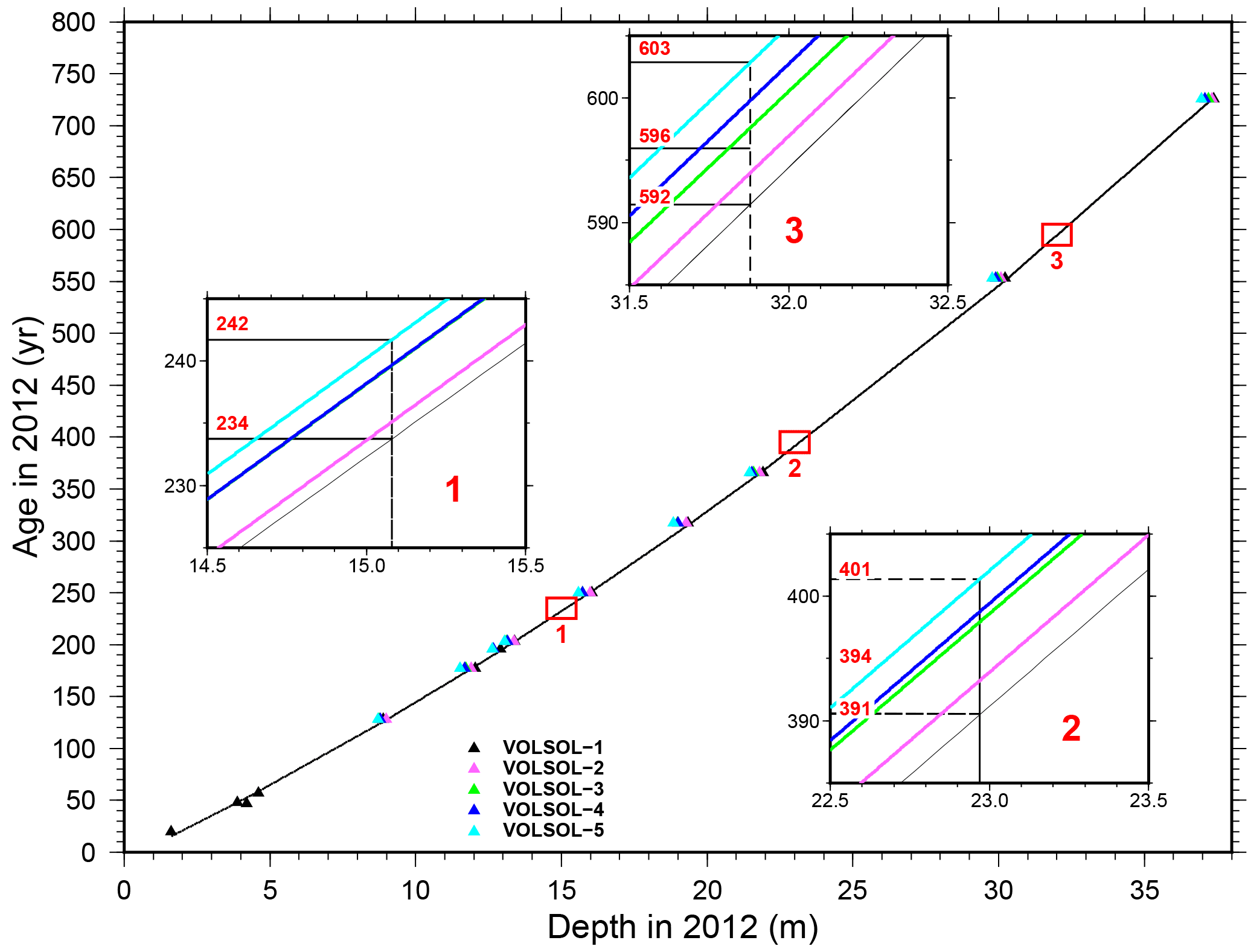
Figure B1Time markers along the five cores as studied in Gautier et al. (2016). The reference core is VOLSOL-1 (see Sect. 4.2) for which the quadratic fit is entirely represented in black, whereas insets represent enlargements where all quadratic fits allow for an assessment of the age dispersion around the reference at the depths of our three IRHs.
The age–depth relationships of the five studied cores in Gautier et al. (2016) are represented in Fig. B1, from which the age differences at our three IRH depths can be inferred.
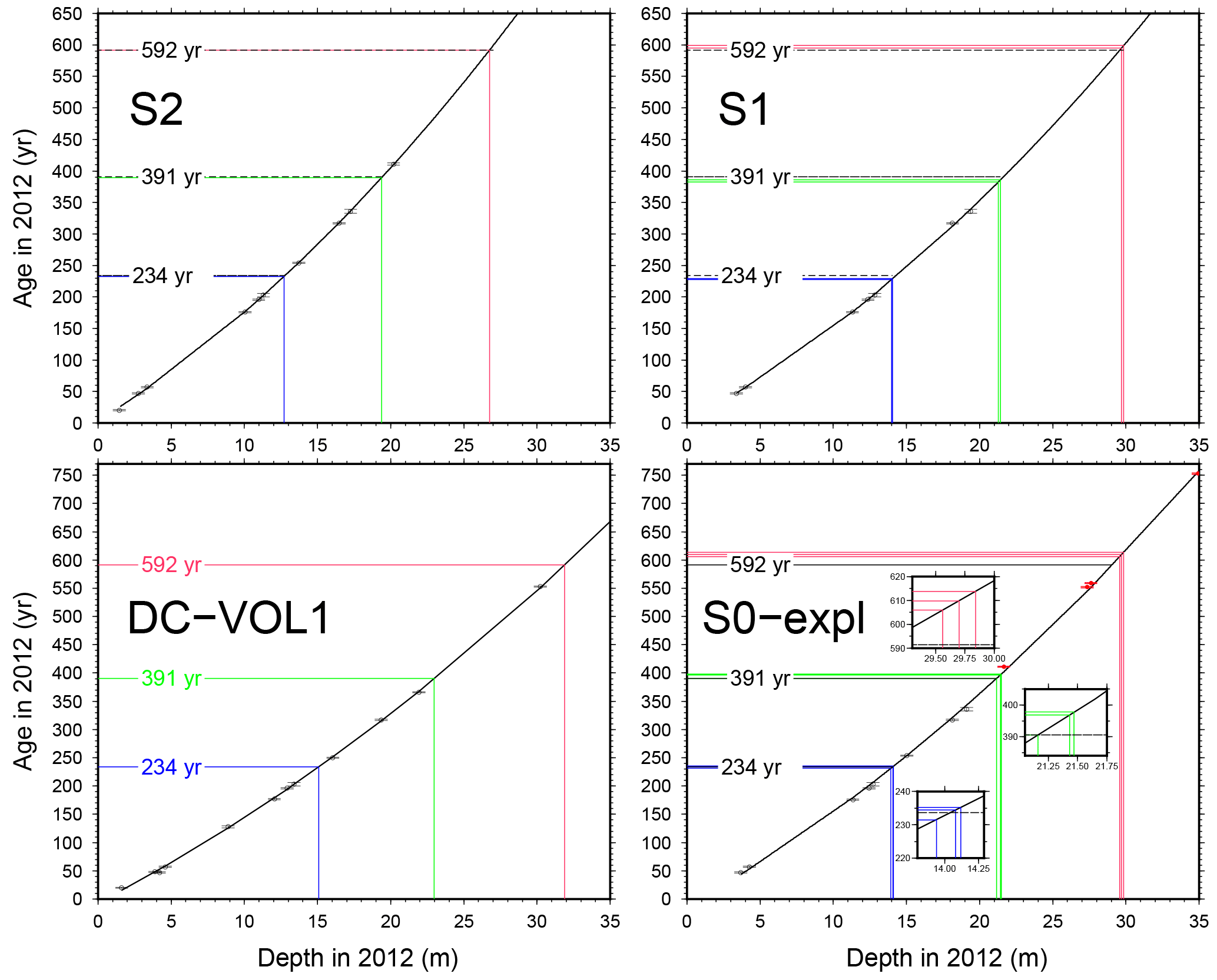
Figure C1Same as Fig. 3 but now including the TASTE-IDEA cores S1 and S2 and the hybrid S0–Explore core. For the latter, extra points issued from the Explore core at larger depths are represented in red.
The consistency and the dispersion for the ages of each of our three IRHs have been assessed by inferring the IRH depths when passing at the various core locations along the radar line. These depths were reported in the corresponding age–depth relationships for the DC-VOLSOL1, S1, S2 and hybrid S0–Explore cores (see Fig. C1).
As can be seen, ages for each IRH remain consistent along the entire radar profile with a limited scatter at the various crossings (either between cores or when passing several times at the same core site). For instance, the uppermost blue IRH varies by only 3 % among all crossing points and has a maximum discrepancy of only 6 years (2.5 %) with the DC reference age (see detailed figures in Table C1).
As for the second IRH (green), the scatter is 16 years (4 %) with a maximum deviation of 9 years from the DC age of 391 years. Lastly, the deepest one (pink) has a maximum deviation of 3.75 % (22 years) from the reference age, which also corresponds to its total dispersion. The only noticeable discrepancy is to be found with the deepest IRH when passing the S0 site, where crossing depths lead to systematically older ages. One explanation could lie in the loss of continuity for this deepest IRH towards the end of the profile, where it sometimes becomes very faint (see bottom right of Fig. 2). The other possibility is that it results from the hybrid depth–age relationship obtained at S0 from two different cores. Because of the short-scale variability of surface snow post-deposition processes (Eisen et al., 2008), the distance of 70 m between the two cores may explain such discrepancies as was observed by Gautier et al. (2016), who found depth shifts of the order of 20 cm between five cores only separated by 1 m at the DC site. They also came to the conclusion that logging errors and analysing procedures may play a role, especially if different coring and analysing teams are involved as was the case for the S0 and Explore cores. Although it can be criticized, the construction of such a hybrid age–depth relationship makes some sense in our case since we only considered the extra Explore markers at depths where no other volcanoes were available in the initial S0 core (> 20 m). The resulting quadratic fit still yields r2 greater than 0.99.
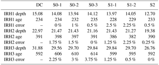
Table C1Depth, corresponding age and deviation with respect to the DC-VOLSOL-1 reference age for the three IRHs whenever they intersect the DC-VOL-1, S0–Explore, S1 and S2 cores
The authors declare that they have no conflict of interest.
We would like to thank the French Research National Agency (Project
ANR-07-VULN-013 VANISH), who provided significant financial support to the
TASTE-IDEA 2010-11 traverse, where data of the present study originate. The
French Polar Institute (IPEV) was crucial in the success of this traverse by
mastering all the logistical aspects and providing the necessary staff,
material, and consumables. The technical staff (IGE: Eric Lefebvre and
Grégory Teste; IPEV: Antony Vende, Alexandre Leluc and David Colin) are
also heartily thanked for their invaluable expertise. The Russian Arctic and
Antarctic Expeditions (AARI, Vostok base) are also thanked for having
welcomed the traverse at the Vostok Station. Projects
“ANR-06-VULN-016-01DACOTA” and “ANR-12-BS06-0018-SUMER” also contributed
by funding a significant part of the GPR used in the present study. Lastly,
we would like to thank the three reviewers, whose suggestions and remarks
considerably improved the manuscript.
Edited
by: Michiel van den Broeke
Reviewed by: Elisabeth Isaksson,
Ian D. Goodwin,
and one anonymous referee
Arthern, R. J., Winebrenner, D. P., and Vaughan, D. G.: Antarctic snow accumulation mapped using polarization of 4.3-cm wavelength microwave emission, J. Geophys. Res., 111, D06107, https://doi.org/10.1029/2004JD005667, 2006. a
Augustin, L., Barbante, C., Barnes, P. R., et al.: Eight glacial cycles from an Antarctic ice core, Nature, 429, 623–628, 2004. a
Bamber, J. L., Gomez-Dans, J. L., and Griggs, J. A.: A new 1 km digital elevation model of the Antarctic derived from combined satellite radar and laser data – Part 1: Data and methods, The Cryosphere, 3, 101–111, https://doi.org/10.5194/tc-3-101-2009, 2009 a, b, c
Bintanja, R.: On the glaciological, meteorological, and climatological significance of Antarctic blue ice areas, Rev. Geophys., 37, 337–359, https://doi.org/10.1029/1999RG900007, 1999. a
Castellano, E., Becagli, S., Jouzel, J., Migliori, A., Severi, M., Steffensen, J., Traversi, R., and Udisti, R.: Volcanic eruption frequency over the last 45 ky as recorded in Epica-Dome C ice core (East Antarctica) and its relationship with climatic changes, Global. Planet. Change, 42, 195–205, https://doi.org/10.1016/j.gloplacha.2003.11.007, 2004. a, b, c, d, e
Cole-Dai, J., Mosley-Thompson, E., and Thompson, L. G.: Annually resolved southern hemisphere volcanic history from two Antarctic ice cores, J. Geophys. Res.-Atmos., 102, 16761–16771, https://doi.org/10.1029/97JD01394, 1997. a
Cole-Dai, J., Mosley-Thompson, E., Wight, S. P., and Thompson, L. G.: A 4100-year record of explosive volcanism from an East Antarctica ice core, J. Geophys. Res.-Atmos., 105, 24431–24441, https://doi.org/10.1029/2000JD900254, 2000. a, b, c, d
Eisen, O., Nixdorf, U., Wilhelms, F., and Miller, H.: Age estimates of isochronous reflection horizons by combining ice core, survey, and synthetic radar data, J. Geophys. Res., 109, B04106, https://doi.org/10.1029/2003JB002858, 2004. a, b, c
Eisen, O., Frezzotti, M., Genthon, C., Isaksson, E., Magand, O., van den Broeke, M. R., Dixon, D. A., Ekaykin, A., Holmlund, P., Kameda, T., Karlöf, L., Kaspari, S., Lipenkov, V. Y., Oerter, H., Takahashi, S., and Vaughan, D. G.: Ground-based measurements of spatial and temporal variability of snow accumulation in East Antarctica, Rev. Geophys., 46, RG2001, https://doi.org/10.1029/2006RG000218, 2008. a, b, c, d, e, f
Fischer, H., Severinghaus, J., Brook, E., Wolff, E., Albert, M., Alemany, O., Arthern, R., Bentley, C., Blankenship, D., Chappellaz, J., Creyts, T., Dahl-Jensen, D., Dinn, M., Frezzotti, M., Fujita, S., Gallee, H., Hindmarsh, R., Hudspeth, D., Jugie, G., Kawamura, K., Lipenkov, V., Miller, H., Mulvaney, R., Parrenin, F., Pattyn, F., Ritz, C., Schwander, J., Steinhage, D., van Ommen, T., and Wilhelms, F.: Where to find 1.5 million yr old ice for the IPICS “Oldest-Ice” ice core, Clim. Past, 9, 2489–2505, https://doi.org/10.5194/cp-9-2489-2013, 2013. a
Frezzotti, M., Pourchet, M., Flora, O., Gandolfi, S., Gay, M., Urbini, S., Vincent, C., Becagli, S., Gragnani, R., and Proposito, M.: Spatial and temporal variability of snow accumulation in East Antarctica from traverse data, J. Glaciol., 51, 113–124, 2005. a, b, c, d
Frezzotti, M., Urbini, S., Proposito, M., Scarchilli, C., and Gandolfi, S.: Spatial and temporal variability of surface mass balance near Talos Dome, East Antarctica, J. Geophys. Res., 112, F02032, https://doi.org/10.1029/2006JF000638, 2007. a, b, c
Frezzotti, M., Scarchilli, C., Becagli, S., Proposito, M., and Urbini, S.: A synthesis of the Antarctic surface mass balance during the last 800 yr, The Cryosphere, 7, 303–319, https://doi.org/10.5194/tc-7-303-2013, 2013. a
Fujita, S., Holmlund, P., Andersson, I., Brown, I., Enomoto, H., Fujii, Y., Fujita, K., Fukui, K., Furukawa, T., Hansson, M., Hara, K., Hoshina, Y., Igarashi, M., Iizuka, Y., Imura, S., Ingvander, S., Karlin, T., Motoyama, H., Nakazawa, F., Oerter, H., Sjöberg, L. E., Sugiyama, S., Surdyk, S., Ström, J., Uemura, R., and Wilhelms, F.: Spatial and temporal variability of snow accumulation rate on the East Antarctic ice divide between Dome Fuji and EPICA DML, The Cryosphere, 5, 1057–1081, https://doi.org/10.5194/tc-5-1057-2011, 2011 a, b
Gao, C., Robock, A., Self, S., Witter, J. B., Steffenson, J. P., Clausen, H. B., Siggaard-Andersen, M., Johnsen, S., Mayewski, P. A., and Ammann, C.: The 1452 or 1453 A.D. Kuwae eruption signal derived from multiple ice core records: Greatest volcanic sulfate event of the past 700 years, J. Geophys. Res., 111, D12107, https://doi.org/10.1029/2005JD006710, 2006. a
Gao, C., Robock, A., and Ammann, C.: Volcanic forcing of climate over the past 1500 years: An improved ice core-based index for climate models, J. Geophys. Res.-Atmos., 113, D23111, https://doi.org/10.1029/2008JD010239, 2008. a
Gautier, E., Savarino, J., Erbland, J., Lanciki, A., and Possenti, P.: Variability of sulfate signal in ice core records based on five replicate cores, Clim. Past, 12, 103–113, https://doi.org/10.5194/cp-12-103-2016, 2016. a, b, c, d, e, f, g
Genthon, C., Six, D., Scarchilli, C., Ciardini, V., and Frezzotti, M.: Meteorological and snow accumulation gradients across Dome C, East Antarctic plateau, Int. J. Climatol., 36, 455–466, https://doi.org/10.1002/joc.4362, 2015. a, b, c
Igarashi, M., Nakai, Y., Motizuki, Y., Takahashi, K., Motoyama, H., and Makishima, K.: Dating of the Dome Fuji shallow ice core based on a record of volcanic eruptions from AD 1260 to AD 2001, Polar Science, 5, 411–420, https://doi.org/10.1016/j.polar.2011.08.001, 2011. a
Kovacs, A., Gow, A. J., and Morey, R. M.: The in-situ dielectric constant of polar firn revisited, Cold Reg. Sci. Technol., 23, 245–256, 1995. a
Krinner, G., Magand, O., Simmonds, I., Genthon, C., and Dufresne, J. L.: Simulated Antarctic precipitation and surface mass balance at the end of the twentieth and twenty-first centuries, Clim. Dynam., 28, 215–230, https://doi.org/10.1007/s00382-006-0177-x, 2006. a
Leduc-Leballeur, Picard, G., Mialon, A., Arnaud, L., Lefebvre, E., Possenti, P., and Kerr, Y.: Modeling L-band brightness temperature at Dome C, Antarctica and comparison with SMOS observations, IEEE T. Geosci. Remote, 53, 4022–4032, https://doi.org/10.1109/TGRS.2015.2388790, 2015. a, b, c, d
Le Meur, E.: Surface mass balance measurements between Dome Concordia and Vostok, East Antarctica, PANGAEA, https://doi.org/10.1594/PANGAEA.890096, 2018. a
Libois, Q., Picard, G., Arnaud, L., Morin, S., and Brun, E.: Modeling the impact of snow drift on the decameter-scale variability of snow properties on the Antarctic Plateau, J. Geophys. Res.-Atmos., 119, 11662–11681, https://doi.org/10.1002/2014JD022361, 2014. a, b, c
Loaiza, P., Chassaing, C., Hubert, P., Nachab, A., Perrot, F., Reyss, J., and Warot, G.: Low background germanium planar detector for gamma-ray spectrometry, Nucl. Instrum. Meth. A, 634, 64–70, https://doi.org/10.1016/j.nima.2011.01.017, 2011. a
Magand, O.: Bilan de masse de surface Antarctique: techniques de mesure et analyse critique, PhD thesis, Citeseer, 2009. a, b, c
Magand, O., Genthon, C., Fily, M., Krinner, G., Picard, G., Frezzotti, M., and Ekaykin, A. A.: An up-to-date quality-controlled surface mass balance data set for the 90–180∘ E Antarctica sector and 1950–2005 period, J. Geophys. Res.-Atmos., 112, D12106, https://doi.org/10.1029/2006JD007691, 2007. a
Maupetit, F. and Delmas, R. J.: Chemical composition of falling snow at Dumont d'Urville, Antarctica, J. Atmos. Chem., 14, 31–42, 1992. a
Mayewski, P. A., Frezzotti, M., Bertler, N., Van Ommen, T., Hamilton, G., Jacka, T. H., Welch, B., Frey, M., Dahe, Q., and Jiawen, R.: The international trans-antarctic scientific expedition (ITASE): an overview, Ann. Glaciol., 41, 180–185, 2005. a
Muller, K., Sinisalo, A., Anschutz, H., Hamran, S., Hagen, J., McConnell, J. R., and Pasteris, D. R.: An 860 km surface mass-balance profile on the East Antarctic plateau derived by GPR, Ann. Glaciol., 51, 1–8, 2010. a, b, c
Osipov, E. Y., Khodzher, T. V., Golobokova, L. P., Onischuk, N. A., Lipenkov, V. Y., Ekaykin, A. A., Shibaev, Y. A., and Osipova, O. P.: High-resolution 900 year volcanic and climatic record from the Vostok area, East Antarctica, The Cryosphere, 8, 843–851, https://doi.org/10.5194/tc-8-843-2014, 2014. a
Palli, A., Kohler, J. C., Isaksson, E., Moore, J. C., Pinglot, J. F., Pohjola, V. A., and Samuelsson, H.: Spatial and temporal variability of snow accumulation using ground-penetrating radar and ice cores on a Svalbard glacier, J. Glaciol., 48, 417–424, 2002. a
Palmer, A. S., van Ommen, T. D., Curran, M. A. J., Morgan, V., Souney, J. M., and Mayewski, P. A.: High-precision dating of volcanic events (A.D. 1301–1995) using ice cores from Law Dome, Antarctica, J. Geophys. Res.-Atmos., 106, 28089–28095, https://doi.org/10.1029/2001JD000330, 2001. a, b
Parrenin, F., Barnola, J.-M., Beer, J., Blunier, T., Castellano, E., Chappellaz, J., Dreyfus, G., Fischer, H., Fujita, S., Jouzel, J., Kawamura, K., Lemieux-Dudon, B., Loulergue, L., Masson-Delmotte, V., Narcisi, B., Petit, J.-R., Raisbeck, G., Raynaud, D., Ruth, U., Schwander, J., Severi, M., Spahni, R., Steffensen, J. P., Svensson, A., Udisti, R., Waelbroeck, C., and Wolff, E.: The EDC3 chronology for the EPICA Dome C ice core, Clim. Past, 3, 485–497, https://doi.org/10.5194/cp-3-485-2007, 2007. a
Patris, N., Delmas, R. J., and Jouzel, J.: Isotopic signatures of sulfur in shallow Antarctic ice cores, J. Geophys. Res.-Atmos., 105, 7071–7078, 2000. a
Plummer, C. T., Curran, M. A. J., van Ommen, T. D., Rasmussen, S. O., Moy, A. D., Vance, T. R., Clausen, H. B., Vinther, B. M., and Mayewski, P. A.: An independently dated 2000-yr volcanic record from Law Dome, East Antarctica, including a new perspective on the dating of the 1450s CE eruption of Kuwae, Vanuatu, Clim. Past, 8, 1929–1940, https://doi.org/10.5194/cp-8-1929-2012, 2012. a
Pourchet, M., Magand, O., Frezzotti, M., Ekaykin, A., and Winther, J.: Radionuclides deposition over Antarctica, J. Environ. Radioactiv., 68, 137–158, https://doi.org/10.1016/S0265-931X(03)00055-9, 2003. a, b
Prospero, J. M., Savoie, D. L., Saltzman, E. S., and Larsen, R.: Impact of oceanic sources of biogenic sulphur on sulphate aerosol concentrations at Mawson, Antarctica, 350, 221–223, https://doi.org/10.1038/350221a0, 1991. a
Rignot, E. and Kanagaratnam, P.: Changes in the Velocity Structure of the Greenland Ice Sheet, Science, 311, 986–990, https://doi.org/10.1126/science.1121381, 2006. a
Röthlisberger, R.: Dust and sea salt variability in central East Antarctica (Dome C) over the last 45 kyrs and its implications for southern high-latitude climate, Geophys. Res. Lett., 29, 1963, https://doi.org/10.1029/2002GL015186, 2002. a, b
Ruth, U., Barnola, J.-M., Beer, J., Bigler, M., Blunier, T., Castellano, E., Fischer, H., Fundel, F., Huybrechts, P., Kaufmann, P., Kipfstuhl, S., Lambrecht, A., Morganti, A., Oerter, H., Parrenin, F., Rybak, O., Severi, M., Udisti, R., Wilhelms, F., and Wolff, E.: “EDML1”: a chronology for the EPICA deep ice core from Dronning Maud Land, Antarctica, over the last 150 000 years, Clim. Past, 3, 475–484, https://doi.org/10.5194/cp-3-475-2007, 2007. a
Saltzman, E. S.: Ocean/Atmosphere Cycling of Dimethylsulfide, in: Ice Core Studies of Global Biogeochemical Cycles, edited by: Delmas, R. J., no. 30 in NATO ASI Series, Springer, Berlin Heidelberg, 65–89, 1995. a
Salzer, M. W. and Hughes, M. K.: Bristlecone pine tree rings and volcanic eruptions over the last 5000 yr, Quaternary Res., 67, 57–68, https://doi.org/10.1016/j.yqres.2006.07.004, 2007. a
Scambos, T., Frezzotti, M., Haran, T., Bohlander, J., Lenaerts, J., van Den Broeke, M., Jezek, K., Long, D., Urbini, S., Farness, K., Neumann, T., Albert, M., and Winther, J.: Extent of low-accumulation “wind glaze” areas on the East Antarctic plateau: implications for continental ice mass balance, J. Glaciol., 58, 633–647, https://doi.org/10.3189/2012JoG11J232, 2012. a
Sigl, M., McConnell, J. R., Layman, L., Maselli, O., McGwire, K., Pasteris, D., Dahl-Jensen, D., Steffensen, J. P., Vinther, B., Edwards, R., Mulvaney, R., and Kipfstuhl, S.: A new bipolar ice core record of volcanism from WAIS Divide and NEEM and implications for climate forcing of the last 2000 years, J. Geophys. Res.-Atmos., 118, 1151–1169, https://doi.org/10.1029/2012JD018603, 2013. a
Sigl, M., McConnell, J. R., Toohey, M., Curran, M., Das, S. B., Edwards, R., Isaksson, E., Kawamura, K., Kipfstuhl, S., Krüger, K., Layman, L., Maselli, O. J., Motizuki, Y., Motoyama, H., Pasteris, D. R., and Severi, M.: Insights from Antarctica on volcanic forcing during the Common Era, Nat. Clim. Change, 4, 693–697, https://doi.org/10.1038/nclimate2293, 2014. a
Sigl, M., Winstrup, M., McConnell, J. R., Welten, K. C., Plunkett, G., Ludlow, F., Büntgen, U., Caffee, M., Chellman, N., Dahl-Jensen, D., Fischer, H., Kipfstuhl, S., Kostick, C., Maselli, O. J., Mekhaldi, F., Mulvaney, R., Muscheler, R., Pasteris, D. R., Pilcher, J. R., Salzer, M., Schüpbach, S., Steffensen, J. P., Vinther, B. M., and Woodruff, T. E.: Timing and climate forcing of volcanic eruptions for the past 2,500 years, Nature, 523, 543–549, https://doi.org/10.1038/nature14565, 2015. a
Simmons, A., Uppala, S., Dee, D., and Kobayashi, S.: ERA-Interim: New ECMWF reanalysis products from 1989 onwards, ECMWF newsletter, 110, 25–35, 2007. a
Stenni, B.: Eight centuries of volcanic signal and climate change at Talos Dome (East Antarctica), J. Geophys. Res., 107, 4076, https://doi.org/10.1029/2000JD000317, 2002. a
Urbini, S., Frezzotti, M., Gandolfi, S., Vincent, C., Scarchilli, C., Vittuari, L., and Fily, M.: Historical behaviour of Dome C and Talos Dome (East Antarctica) as investigated by snow accumulation and ice velocity measurements, Global Planet. Change, 60, 576–588, https://doi.org/10.1016/j.gloplacha.2007.08.002, 2008. a, b, c, d, e, f, g, h, i, j, k, l
van den Broeke, M., van de Berg, W. J., and van Meijgaard, E.: Snowfall in coastal West Antarctica much greater than previously assumed, Geophys. Res. Lett., 33, L02505, https://doi.org/10.1029/2005GL025239, 2006. a
van den Broeke, M. R., Bamber, J., Lenaerts, J., and Rignot, E.: Ice Sheets and Sea Level: Thinking Outside the Box, Surv. Geophys., 32, 495–505, https://doi.org/10.1007/s10712-011-9137-z, 2011. a
Vaughan, D. G., Anderson, P. S., King, J. C., Mann, G. W., Mobbs, S. D., and Ladkin, R. S.: Imaging of firn isochrones across an Antarctic ice rise and implications for patterns of snow accumulation rate, J. Glaciol., 50, 413–418, 2004. a
Verfaillie, D., Fily, M., Le Meur, E., Magand, O., Jourdain, B., Arnaud, L., and Favier, V.: Snow accumulation variability derived from radar and firn core data along a 600 km transect in Adelie Land, East Antarctic plateau, The Cryosphere, 6, 1345–1358, https://doi.org/10.5194/tc-6-1345-2012, 2012. a, b, c, d, e
- Abstract
- Introduction
- Ground-penetrating radar (GPR) data
- Ice core data
- IRH dating
- Snow accumulation along the GPR profile
- Accumulation space and time distribution
- Conclusions
- Data availability
- Appendix A: Ice core sampling and analysis
- Appendix B: Ice core representativeness
- Appendix C: Age dispersion along the radar line
- Competing interests
- Acknowledgements
- References
The requested paper has a corresponding corrigendum published. Please read the corrigendum first before downloading the article.
- Article
(3438 KB) - Full-text XML
- Abstract
- Introduction
- Ground-penetrating radar (GPR) data
- Ice core data
- IRH dating
- Snow accumulation along the GPR profile
- Accumulation space and time distribution
- Conclusions
- Data availability
- Appendix A: Ice core sampling and analysis
- Appendix B: Ice core representativeness
- Appendix C: Age dispersion along the radar line
- Competing interests
- Acknowledgements
- References