


1. Introduction
Break-offs from hanging glaciers can release large volumes of ice into the valleys below. The consequences of serac falls are generally limited to high mountain areas and the related risks are often restricted to mountaineers only. However, in densely populated mountainous areas such break-offs can have catastrophic consequences for life and property (Reference Haeberli, Alean, Müller and FunkHaeberli and others, 1989). The two most serious ice avalanche catastrophes occurred below the Huascarán mountain summit in the Peruvian Andes in 1962 and 1970, killing 4000 and 20 000 people, respectively (Reference LliboutryLliboutry, 1975). In 1965, the tongue of Allalin glacier, Switzerland, broke off and killed 88 people working on the construction of the Mattmark dam (Reference RöthlisbergerRöthlisberger, 1981). In 2002, a huge snow/ice avalanche triggered a mudflow that killed 120 people in the Russian Caucasus (Reference Kääb, Wessels, Haeberli, Huggel, Kargel and KhalsaKääb and others, 2003; Reference HaeberliHaeberli and others, 2004). The rupture of Altels glacier, Switzerland, in 1895 led to a huge ice break-off with a released volume of ~4 × 10⁶m3, killing six people (Reference ForelForel, 1895; Reference Röthlisberger and KasserRöthlisberger and Kasser, 1978; Reference RöthlisbergerRöthlisberger, 1981). Other glaciers have produced icefalls in the past that have led to huge ice avalanches without causing fatalities. However, such glaciers remain a threat to the populations in the valleys below. This is the case for Weisshorn glacier, Switzerland, from which there have been five break-offs since 1973 (Reference Raymond, Wegmann and FunkRaymond and others, 2003). Similarly, Grandes Jorasses hanging glacier, Italy, triggered an ice avalanche of 150 000 m3 in 1998 that reached the bottom of the valley (Reference Margreth, Faillettaz, Funk, Vagliasindi, Diotri and BroccolatoMargreth and others, 2011).
For these reasons, reliable tools to quantify and predict such events are required to protect populations at risk (Reference FlotronFlotron, 1977; Reference Pralong, Birrer, Stahel and FunkPralong and others, 2005; Reference Pralong and FunkPralong and Funk, 2006; Reference Faillettaz, Pralong, Funk and DeichmannFaillettaz and others, 2008, Reference Faillettaz, Sornette and Funk2010, Reference Faillettaz, Funk and Sornette2011a). Reference Faillettaz, Sornette and FunkFaillettaz and others (2010, Reference Faillettaz, Funk and Sornette2011a,Reference Faillettaz, Sornette and Funkb, Reference Faillettaz, Funk and Sornette2012) identified several types of instability according to the thermal properties of the ice/bed interface. They discuss possible precursory signs for each type of instability, although the prediction of such events remains problematic for temperate and partly temperate basal conditions. For glaciers frozen to bedrock on very steep slopes, such as Weisshorn and Grandes Jorasses glaciers, monitoring techniques have been implemented to predict large break-offs. These methods are based on the surface displacement, which exhibits a power law acceleration with log-periodic oscillations (Reference LüthiLüthi, 2003; Reference Pralong, Birrer, Stahel and FunkPralong and others, 2005; Reference Faillettaz, Pralong, Funk and DeichmannFaillettaz and others, 2008), and on the seismic activity generated by the glacier before a large break-off (Reference Faillettaz, Funk and SornetteFaillettaz and others, 2011a). The seismic monitoring revealed three regimes corresponding to different fracture processes that can be used as precursory signs to predict a large break-off (Reference Faillettaz, Funk and SornetteFaillettaz and others, 2011a). Other glacier instabilities are related to the presence of water located at the ice/bedrock interface of steep temperate glaciers. The subglacial drainage network plays a key role in such events (Reference Dalban Canassy, Faillettaz, Walter and HussDalban Canassy and others, 2012; Reference Dalban Canassy, Faillettaz, Walter and HussFaillettaz and others, 2012). If the drainage network is distributed, a pulse of subglacial water flow may lead to a sudden increase in water pressure and can affect the stability of the glacier tongue. Moreover, it seems that a major break-off can occur only if the water pulse is preceded by a decrease in subglacial runoff (Reference Dalban Canassy, Faillettaz, Walter and HussFaillettaz and others, 2012).
The aim of this paper is to examine Taconnaz hanging glacier, Mont Blanc area, French Alps, where icefall events threaten inhabited areas in the valley of Chamonix. The basal ice of this glacier is cold (see Section 5). At this location icefalls are a particular risk during winter when the snow mantle is unstable. At such times, huge ice blocks breaking off the ice cliff can trigger large avalanches carrying a mixture of snow and ice. The avalanche of 20 March 1988 devastated some inhabited areas but did not cause fatalities. Large avalanche protection dams and deflecting concrete walls were built in 1986 and 1990 to protect the village of Le Nant. A large avalanche of snow and ice, very likely triggered by an icefall, occurred on 11 February 1999 (Reference Le Meur and VincentLe Meur and Vincent, 2006). The avalanche passed over the dam and stopped on a ski run, very close to inhabited areas. Fortunately, nobody was in this area at the time. The volume of the avalanche in 1999 was assessed at ~750 000 m3. In 2010, public authorities decided to modify the passive defense structure (dam height, new retarding mounds) to increase the safety of the inhabited area (Reference Naaim, Faug, Naaim and EckertNaaim and others, 2010).
In a previous study (Reference Le Meur and VincentLe Meur and Vincent, 2006) changes in the position of the ice-cliff edge were obtained from topographic surveys performed at Aiguille du Midi and Plan de l’Aiguille between 13 February 2002 and 8 December 2003. These measurements, carried out every 3 or 4 weeks, were used to compute the average positions of the two differently oriented parts of the cliff as a function of time. From these observations, Reference Le Meur and VincentLe Meur and Vincent (2006) noted several major collapses that occurred once the cliff edge reached a threshold position. In addition, they observed a period of ~ 180 days between these major icefalls. However, they noted that this period could be simply a coincidence for the observed collapses. They recognized that the approach suffered from uncertainties in both the exact time of the collapses and the associated falling volumes. Therefore Reference Le Meur and VincentLe Meur and Vincent (2006) recommended improving the survey protocol with more frequent observations from daily remote photographs using photogrammetric methods. They concluded that it might be possible to detect a risky situation whenever one of the two cliff portions advances up to a characteristic limit in the presence of a deep and unstable winter snow mantle.
The aims of this paper are to (1) assess the volume and frequency of large collapses and (2) determine an indicator of large collapses. This paper aims to obtain more accurate data on ice volume changes using the photogrammetric method with daily photographs. The ultimate goal is to confirm or invalidate previous results on the characteristic thresholds for large collapses and the possibility of detecting a risky situation.
2. Site Characteristics
Taconnaz glacier is located on the north face of the Mont Blanc massif in the valley of Chamonix. It consists of an upper accumulation area of ~2 km2 below Dôme du Goûter. Along its path, the ice flow concentrates and a large part of the accumulated ice is channeled through a ~600 m wide ice cliff at ~3300 m a.s.l. (Fig. 1). The basal ice of the accumulation zone is cold (Reference Gilbert and VincentGilbert and Vincent, 2013). The cliff has two parts distinguished by different orientations, one facing north and the other northwest. Access to the upper part of the glacier is problematic, and only possible from the top of the glacier, and therefore requires helicopter transportation. Moreover, the accumulation zone has several serac zones and crevasse areas that prevent easy access and long stays. Consequently, in situ measurements are limited and remote-sensing techniques are preferable.

Fig. 1. Aerial view of Taconnaz glacier showing the icefall and the avalanche defense structure downstream in the valley to protect the inhabited area. The photogrammetric stations used in this study are located 3750 m from the ice cliff on each end of the 236 m red baseline near Cosmiques hut.
3. Data and Methods
From 13 February 2002 to 8 December 2003 topographic surveys of the ice-cliff edge were performed from two topographic stations every 3–4 weeks to infer position changes. The topographic stations were located ~4.2 km from the ice cliff. The monitoring was based on an intersection method, with no recourse to distance measurements (Reference Le Meur and VincentLe Meur and Vincent, 2006). This method is very effective although time-consuming. It was used for the icecliff edge survey only and could not be used to obtain a digital elevation model (DEM) of the icefall.
To obtain a more exhaustive set of measurements, terrestrial photogrammetric surveys have been carried out over recent years. Photographs were taken every 2 hours between 30 April 2010 and 15 April 2011 from two stations located near the Cosmiques hut (Fig. 1). Two additional photogrammetric surveys were carried out on 4 and 10 May 2012, before and after a large ice avalanche. The photographs were automatically triggered using two Canon EOS 5D Mark II digital reflex cameras with Canon 100 mm f/2.8 AF fixed-focus lenses. The 21.1 × 106 pixel images are captured in RAW uncompressed format. The cameras are powered by 12V batteries, solar panels and a regulated 7.4 V (15 W) power supply. As a non-metric system is used to retrieve measurements, calibration is required. The distortion of the lens, the principal point and the focal length were measured. We found a non-negligible negative pincushion distortion reaching 119 μ m at corners (–0.55%), which is typical for long focal length lenses. For correct scaling of the images, we account for the exact focal length (99.57 mm). The radial shift (decentration) of the perspective center (251 μm, i.e. 39 pixels) is also taken into account in the camera model. The two cameras are located at 3609 and 3600 m a.s.l., respectively, and 3750 m from the ice cliff, which results in a ground-scaled pixel of 0.27 m. The cameras are 236 m apart and the base formed by the cameras is approximately perpendicular to the sightings. The base-to-distance ratio is 6.3%, which enables an acceptable stereovision for manual plotting during restitution. In order to orient the images, a preliminary stereopreparation was performed using geodetic differential GPS (DGPS) on six control points (Fig. 2). Large white painted crosses of 2 m × 2 m were used as control points. Moreover, about 150 tie points were added to the common images to improve consistency. Photogrammetric restitutions were obtained using ArcGIS and ERDAS Stereo Analyst software. Orientation was performed with Leica LPS software. The orientation calculations were carried out within an uncertainty of 0.16 m in XYZ, i.e. nearly half of the pixel size set at ground scale. Using the approach developed by Reference Thibert, Blanc, Vincent and EckertThibert and others (2008), we estimate the accuracy of the photogrammetric restitution at 1 m under good conditions. However, due to shadows and snow cover, comparison between different surveys on fixed areas (rocky parts) reveals an uncertainty of ±2 m (see Section 4.2).

Fig. 2. Map of the upper part of Taconnaz glacier. The bold blue line represents the ice cliff (only four of the six control points are visible). The red dots are boreholes. The blue triangles correspond to the control points used for photogrammetry. The datum line used to measure the position of the ice-cliff edge is shown in red.
Numerous difficulties due to the very cold conditions, clouds and low solar radiation during the winter prevented us from obtaining a regular survey. Owing to these harsh weather conditions and breakdowns, numerous pictures were unavailable or unusable. Nine pairs of images were restituted between 30 April 2010 and 15 April 2011, corresponding to an average time interval of 44 days (Fig. 3).
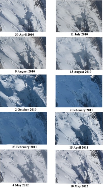
Fig. 3. Photographs of the icefall taken between 30 April 2010 and 10 May 2012.
In a previous study (Reference Le Meur and VincentLe Meur and Vincent, 2006), only icecliff position changes were measured and a simple glacier shape in the form of a parallel-sided slab was assumed. Here photogrammetric methods allow us to accurately calculate the volume changes. Given that large areas are hidden from the photogrammetric stations due to the oblique view, it was not possible to make photogrammetric measurements over a regular horizontal grid. To mitigate this problem, photogrammetric elevation measurements were performed lengthwise along regularly spaced lines to obtain longitudinal surface elevation profiles. Volume changes were calculated from changes in these profiles.
In addition, radar measurements from a helicopter were performed on 7 April 2011 to measure ice thicknesses on the upper part of the glacier. Ground-penetrating radar (GPR) measurements were carried out by the German company RST using a 50–150 MHz shielded antenna connected to a HERA-G/GPR system. The system was mounted directly on the bottom of a helicopter. Signals were recorded with a constant time increment of 0.05 s. GPR signal positions were provided by a synchronized DGPS. Due to the presence of numerous crevasses on the upper eastern part of the glacier, GPR images showed numerous reflections (mainly large scattering), making it difficult to follow the continuity of the glacier/bedrock interface. A wave propagation velocity of 16.8 cm ns–1 within the glacier was used for calculations (Reference Hubbard and GlasserHubbard and Glasser, 2005). Laser scanning surveys from the helicopter were carried out on 11 August 2011 to obtain the surface topography. An LMS-Q560 scanning system was mounted on the bottom of a helicopter equipped with DGPS and inertial measurement unit to derive its position and orientation. The average point density was 6 m–2. Moreover, four hot-water drillings were carried out on 1 and 2 July 2008 from the surface to bedrock between 4080 m a.s.l. and a site located at 3415 m from the ice cliff (Fig. 2). Thermistors with 0.05°C accuracy were installed in the boreholes after drilling was completed. Englacial temperatures were measured on 28 August 2008, i.e. ~2 months after completion of drilling. The goal of these measurements was to assess basal ice temperature in the part of the glacier located upstream of the icefall. Moreover, glacier thickness at each of the borehole locations was used as an additional constraint to construct the DEM of the bedrock
4. Results
4.1. Ice-cliff position changes
Ice-cliff position changes were obtained from photogrammetric surveys performed between April 2010 and April 2011. The photogrammetric measurements focus on the 150 m wide right stream of the glacier, designated as the ‘North Cliff’ by Reference Le Meur and VincentLe Meur and Vincent (2006). The ice cliff of the left stream was not visible from the photogrammetric stations and therefore could not be investigated properly. A protocol similar to that used for topographical surveys (Reference Le Meur and VincentLe Meur and Vincent, 2006) was used to calculate the average position of the cliff edge at different points in time. We did not use exactly the same datum line as that used to calculate the position changes in the 2006 study because the right side of the old datum line was not fully visible from the photogrammetric stations. However, the same method was used to determine the mean position of the ice cliff, which is calculated from the surface area between the edge of the ice cliff and the datum line divided by the width of the cliff (Fig. 2). Nine photogrammetric surveys were performed between April 2010 and April 2011. During this period, one major collapse was observed on 11 August 2010. As also shown by Reference Le Meur and VincentLe Meur and Vincent (2006), Figure 4 reveals a steady advance of the cliff average position up to a threshold position followed by a recession to a minimal position indicating a major collapse. We found minimal and maximal positions very similar to those reported by Reference Le Meur and VincentLe Meur and Vincent (2006). However, Figure 4 shows a complicated pattern after 2 February 2011. Between 2 February and 15 April 2011 although the ice cliff was close to the threshold position no large collapse was observed. Unfortunately, the next available photogrammetric survey was performed on 23 February 2011 and the large gap of 21 days does not allow us to draw a firm conclusion on how the ice discharged. Nevertheless, on 23 February the ice-cliff position is very far from the minimal position and it is probable that the glacier disintegrated continuously into small ice blocks between 2 and 23 February. The longitudinal surface elevation profile measurements and resulting volume changes (Section 4.2) provide a more accurate assessment of geometric changes.
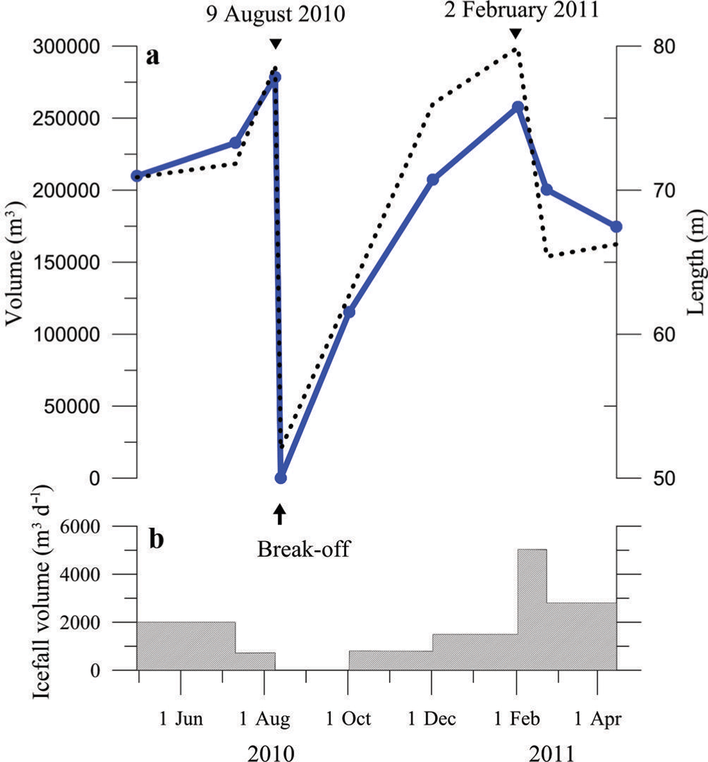
Fig. 4. (a) Averaged ice-cliff positions (dotted line) with respect to the datum line and volume changes (solid line) between 30 April 2010 and 15 April 2011. The volume changes are calculated from the DEM of 13 August 2010. (b) Daily average ice break-off volumes for each survey period.
4.2. Volume changes obtained from longitudinal elevation profile changes
Volume changes were calculated from eight longitudinal surface elevation profiles along which photogrammetric elevation measurements were performed every 10 m. These profiles, about 100–150 m long, were located 20 m apart and were selected in order to be visible on each pair of photographs. In this way, the entire area affected by volume change due to collapse, from the upper part of the serac zone to the bottom of the ice cliff, is covered by a rectangular irregular network of measurement points the average density of which is about one per 20 m2. Figure 5 shows profile 2 for selected dates and reveals very large thickness changes between 9 and 13 August 2010. It also shows that the shape of the ice cliff changed in a complex way. The foot of the cliff is rocky and allows us to assess the uncertainty of photogrammetric surveys: the value found was ±2 m.
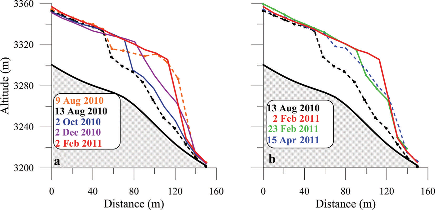
Fig. 5. Longitudinal elevation profile 2 for selected dates between (a) 9 August 2010 and 2 February 2011 and (b) 2 February and 15 April 2011. The bedrock is represented by the bold black line.
DEMs for each survey were obtained from measurements using kriging on a regular grid of 2 m. The volume changes were obtained from DEM differencing. Figure 6 shows the DEM differences for two large collapses. The volume changes between 9 and 13 August 2010 shown in Figure 6a correspond to the large volume collapse observed on 11 August 2010. The total volume change was 278 500 m3 between the two surveys. The maximum height of collapsed ice blocks reached 62 m. The second volume change (Fig. 6b) was obtained for the large ice avalanche that occurred on 7 May 2012. The volume change was determined from the photogrammetric surveys of 4 and 10 May 2012. The total volume change was 273 200 m3 and the maximum height of ice blocks reached 71 m. Like the volume changes, the geometric patterns of these ice collapses are very similar. The topographic surfaces before these major collapses were very similar. The volume changes with time are reported in Figure 4. As already seen for the length fluctuations, it seems that a threshold volume is required to trigger a large ice collapse. However, as mentioned for the length fluctuations, although the glacier reached a position close to the threshold position in February 2011, no large collapse was observed. The glacier likely disintegrated into small ice blocks.
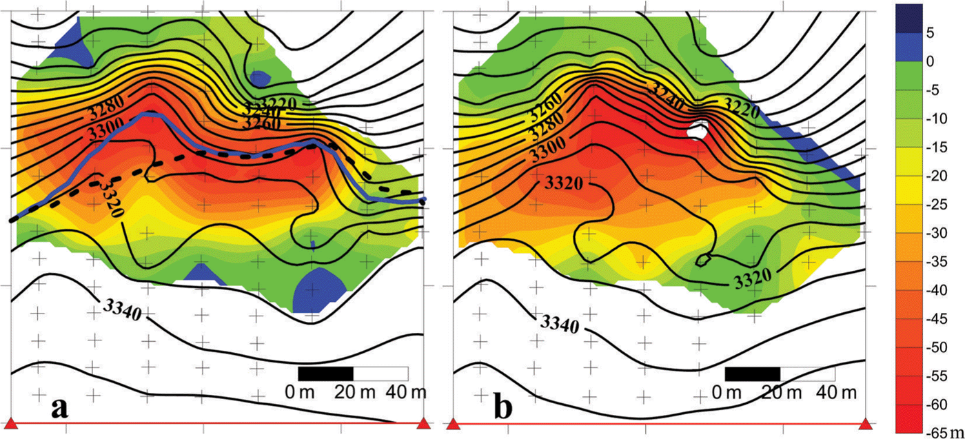
Fig. 6. Thickness changes due to the major collapses of (a) 11 August 2010 and (b) 7 May 2012 obtained from DEM differencing from 9 to 11 August 2010 and 4 to 10 May 2012. The plotted DEM contours (10 m intervals) are before the collapses (9 August 2010 and 4 May 2012, respectively). The measurement datum line, which is used to calculate the ice-cliff position changes, is shown in red. The cliff edge positions of 9 August 2010 and 1 October 2002 are shown in blue (bold line) and black (dashed line), respectively, in (a). The locations of the eight longitudinal profiles are shown as black crosses.
Note that the volume fluctuations show an evolution similar to the fluctuations in ice-cliff position (Fig. 4). The large observed position changes correspond to large volume changes, although the ratio between the two is not constant due to the shape of the tongue, which is not constant. There is clearly no linear relationship between the volume changes and length fluctuations. From this analysis, it can be concluded that a critical geometry, represented by a threshold position or volume, is a necessary condition for triggering a large break-off.
4.3. Ice flux assessments and derived collapse ice volumes
Ice break-off volumes are calculated from the volume changes and the ice flux. The ice flux was assessed in two ways. Firstly, we calculated the maximum rate of volume change between two surveys. For the two measurement periods 11 July–9 August 2010 and 13 August–2 October 2010 the rates of volume change are 2300 and 2350 m3 d–1, respectively. For the second period, which follows the major collapse of 11 August 2010, the thickness change measurements show positive values over the whole area, so we can assume that the ice break-off volumes are negligible during this period. Consequently the observed thickness changes are due to the ice flux only. Therefore, the rate of the volume change observed during this period should correspond approximately to the ice flux of this ice stream. The influence of surface ablation on volume change can be neglected given the large total volume change and the uncertainties. From this analysis, ice flux through the 150 m wide ice stream studied was assessed at 857 750 ± 120 000 m3 a–1.
Secondly, the ice flux was estimated by numerical ice flow modeling. The thermomechanical model used was a full-Stokes thermomechanical model including firn rheology. This ice flow model is based on the work of Reference Zwinger and MooreZwinger and Moore (2009), Reference Lüthi and FunkLüthi and Funk (2000, Reference Lüthi and Funk2001), Reference Gagliardini and MeyssonnierGagliardini and Meyssonnier (1997) and Reference Gilbert, Gagliardini, Vincent and WagnonGilbert and others (in press). Sliding is neglected given that the glacier is cold upstream of the ice cliff (Fig. 7), indeed the basal ice temperature is –11°C at 4080 m a.s.l. (Fig. 7a). Higher basal temperatures have been measured downstream (Fig. 7b and c), but the ice/bedrock interface temperature remains low (close to –2.5°C) at 3415 m a.s.l. (Fig. 7d) in the vicinity of the ice cliff. Ice thicknesses were determined from helicopter-borne radar measurements and adjusted on the basis of the measured thicknesses in the five boreholes. Flow simulations were performed assuming a steady-state temperature field, and took into account coupling between temperature and ice/firn viscosity. The surface ice flow velocity is 78 m a–1 ~200 m upstream of the ice cliff (Reference Le Meur and VincentLe Meur and Vincent, 2006). The flow rate factor was adjusted to match surface velocity measurements from ground GPS observations and SPOT5 (Satellite Pour l’Observation de la Terre) satellite image correlation between 23 August and 8 September 2003 (Reference BerthierBerthier and others, 2005). Given that the basal ice is frozen to the bedrock and the thickness changes are very small above 3300 m a.s.l. (Reference Vincent, Harter, Gilbert, Berthier and SixVincent and others, 2014), we can assume that the ice flow velocity has not changed significantly over the last decade. The resulting ice flux through the studied ice stream is equal to 790 000 ± 100 000 m3 a–1.
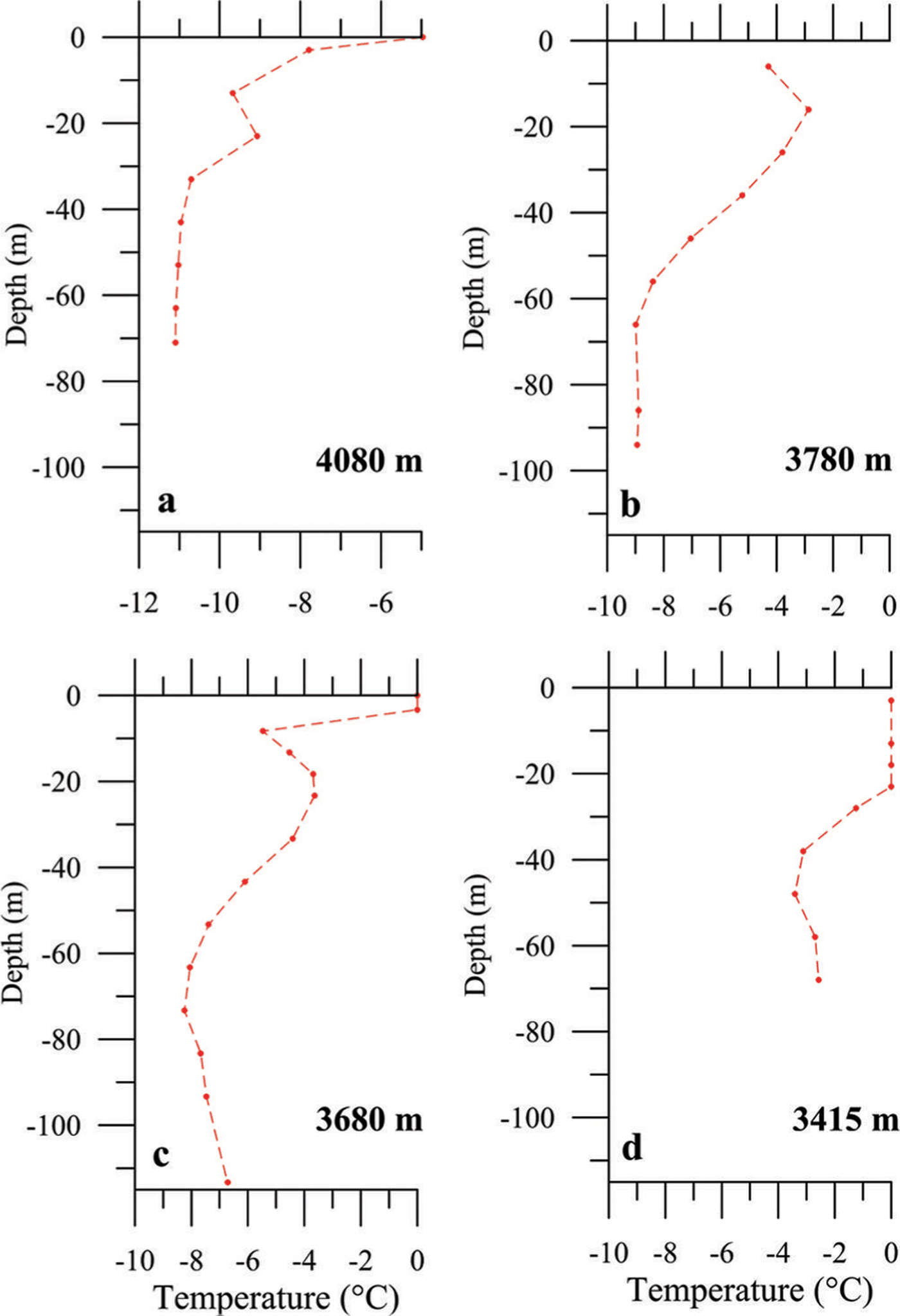
Fig. 7. Boreholes drilled for englacial temperature measurements on Taconnaz glacier at (a) 4080, (b) 3780, (c) 3680 and (d) 3415 m a.s.l.
Finally, for each survey period, the volume of ice break-offs was derived from the ice flux estimations and volume changes (Fig. 4). The ice flux was subtracted from the volume change rate. For each period we used the value of the observed volume change and the value of the daily ice flux obtained previously (2300 m3 d–1). The ice volume breaking off between 9 and 13 August 2010 is not reported in Figure 4 given that it corresponds to a large collapse of 278 500 m3 instantaneously on 11 August 2010. The average break-off rate of the other periods ranges from 0 to 5000 m3 d–1.
5. Discussions and Conclusions
Although the photogrammetric surveys were not carried out continuously due to the harsh conditions often prevailing at this altitude, the volume changes of two major collapses were measured accurately in August 2010 and May 2012. Note that the volume changes related to these two events are very similar and equal to about 275 000 m3. Each of these sudden major collapse volumes is >30% of the annual ice flux through the studied ice stream. This illustrates the importance of the largest collapses in the dynamics of Taconnaz hanging glacier. As for the ice-cliff position changes, we found a threshold volume between the datum line and the ice cliff that cannot be exceeded by the glacier. Consequently, the ice cliff fluctuates between two threshold positions or volumes. In a previous study on position changes alone, Reference Le Meur and VincentLe Meur and Vincent (2006) found two major collapses that occurred once the ice cliff reached a threshold position. In order to compare the threshold positions reached in this study with those reached in the previous study, the cliff edge positions on 9 August 2010 and 1 October 2002 are plotted in Figure 6a. We found very similar threshold positions, indicating that the position has not changed over the last decade. However, in February 2011, the position and volume reached the threshold values without triggering a very large collapse. Consequently, this critical geometry represented by the threshold values is not a sufficient condition. Reference Le Meur and VincentLe Meur and Vincent (2006) reported a period of 180 days between two major collapses. In the present study, a similar period (175 days) was found between the minimal threshold position after the large collapse of 11 August 2010 and the maximal threshold position. This period remains approximate given that we do not know exactly when the collapse occurred after 2 February 2011. However, the time required for the ice cliff to advance from the minimal to the maximal position, where it reaches its critical geometry, is very similar to the period found in 2002 and 2003 (Reference Le Meur and VincentLe Meur and Vincent, 2006). From our analysis, we conclude that this critical geometry is a necessary but not sufficient condition for large break-offs. Indeed, in some cases, although the ice cliff reached the threshold position and volume, the glacier disintegrated into small ice blocks without any large break-off. Consequently, geometric changes in the ice cliff could be a precursory sign of instability of this hanging glacier, but are probably not sufficient conditions for a major break-off.
As a result, a period of 175 days cannot be considered a cyclic return period and used to predict a major collapse. Note that the ice cliff can remain close to the maximal position for several months without triggering a large break-off, as was the case after 2 February 2011. Reference Le Meur and VincentLe Meur and Vincent (2006) observed a similar evolution between June and September 2002 (fig. 9 in Reference Le Meur and VincentLe Meur and Vincent, 2006). During these periods, given that the ice flux is continuous, the serac zone evolves, with frequent falls of small-sized blocks. Note that a large collapse occurred on 7 May 2012 (i.e. 387 days after the end of our measurements on 15 April 2011) when the ice cliff was not very far from the threshold position. We could conclude that two large collapses should have occurred between these two dates, the first at the beginning of May 2011 and the second at the beginning of November 2011. However, such a conclusion remains very speculative.
The behavior of Taconnaz glacier is very different from that of Weisshorn and Grandes Jorasses hanging glaciers. Indeed the ice flux of Taconnaz glacier is much greater and the ice flow velocities are higher. The observed ice flow velocity is close to 80 m a–1 ~200 m upstream of the cliff edge (Reference Le Meur and VincentLe Meur and Vincent, 2006) and we observed an acceleration to >200 m a–1 in the vicinity of the break-off zone. In previous studies of Weisshorn and Grandes Jorasses hanging glaciers, it has been shown that, prior to collapsing, calving blocks are subject to an acceleration indicative of a destabilization process (Reference FlotronFlotron, 1977; Reference Pralong, Birrer, Stahel and FunkPralong and others, 2005; Reference Faillettaz, Pralong, Funk and DeichmannFaillettaz and others, 2008). This acceleration is also visible for Taconnaz glacier in the study of Reference Le Meur and VincentLe Meur and Vincent (2006, their fig. 6). This ice flow acceleration could therefore be a precursory sign of a major break-off of the Taconnaz icefall, as found for the Weisshorn and Grandes Jorasses glaciers. However, the ice flow velocity can be very different depending on the stake locations, and meaningful velocity monitoring would require an extensive network of stakes which would be very difficult to maintain in this area. Moreover, an acceleration could be indicative of a small destabilized volume only. For these reasons, in the case of Taconnaz glacier, we believe that it is preferable to measure the geometry changes of the serac zone, which provides good information on the threshold volume, even if this is not a sufficient condition for a major break-off.
Two values of annual ice flux through the ice stream were estimated using the maximum rate of volume changes and numerical ice flow modeling. These values are in agreement and equal to ~820 000 ± 100 000 m3 a–1. From this value of ice flux, the daily volume of ice breaking off was inferred and ranges from 0 to 5000 m3 d–1 for the surveyed periods except for the major collapse. From the volume of major collapses (275 000 m3) and the annual ice flux, a major collapse would be expected three or four times a year. This is an upper limit for the occurrence of major collapses given that numerous small or moderate collapses occur throughout the year.
Only major ice collapses during winter in the presence of an unstable snow mantle threaten inhabited areas in the valley below. The prediction of major collapses remains a challenge. From the present study we conclude that volume change is the best indicator for break-off prediction, but the threshold volume is not a sufficient condition for triggering a large ice avalanche.
Further studies are necessary to understand the conditions of large instabilities. Ground laser-scanning surveys have been carried out recently to determine more accurately the geometric shape of the glacier with time. Improvements in this technique now make it possible to use it at a distance of 3 km, as required for this icefall. Unfortunately, access is only possible by helicopter and therefore, for economic reasons, it is not possible to perform daily laser-scanning surveys. Consequently, we plan to set up a webcam at the Cosmiques hut to monitor the advance and collapse of the glacier and decide on the best times for laser-scanning surveys.
Another question concerns the englacial temperature rise. A strong englacial temperature increase has been measured since the beginning of the 1990s at Col du Dôme at the summit of Taconnaz glacier (Reference Vincent, Le Meur, Six, Possenti, Lefebvre and FunkVincent and others, 2007; Reference Gilbert and VincentGilbert and Vincent, 2013) and can be attributed to the effect of atmospheric warming. This warming could have a major impact on the stability of hanging glaciers frozen to their beds if the melting point is reached (Fig. 7). As seen in this study, temperatures at the bottom of boreholes on Taconnaz glacier have not yet been affected. However, if the bedrock reaches the pressure-melting point in the future, the stability of this hanging glacier will likely be strongly affected. The presence of water could allow sliding at some locations and decrease basal friction, and lead to a very large ice break-off volume as was the case for Altels glacier in 1895 (Reference Faillettaz, Funk and SornetteFaillettaz and others, 2011b). Numerical modeling studies of coupled heat transfer and ice flow are underway to accurately assess the evolution of temperature in this cold hanging glacier. Taconnaz glacier requires close monitoring of volume changes and englacial temperatures in the future.
Acknowledgements
We thank Frédéric Ousset and Xavier Ravanat (IRSTEA) whose efforts in relation to the photographic system and field measurements contributed greatly to the quality of the datasets. This study was funded by the GlaRiskAlp Alcotra Programme and AQWA European Programme (212250). We thank Philippe Possenti and Luc Piard for conducting the drilling operations, Etienne Berthier for the calculations of ice flow velocities from SPOT5 (Satellite Pour l’Observation de la Terre) images, Harvey Harder who revised the English of the manuscript, and J. Faillettaz and P. Dalban Canassy whose comments improved the quality of the manuscript.


