


 increase sharply at 3000 m.a.s.l. on the plateau, confirming the results of
 1. Introduction
The interpretation of the deuterium and oxygen-18 composition of the snow layers successively deposited over the Greenland and Antarctic ice sheets provides a very powerful tool for reconstructing climatic changes in polar regions.
These profiles primarily contain information related to temperature as there is, for high-latitude present-day precipitation, a well-obeyed linear relationship between surface temperature and either δD or δ 18O. This approach has been used for more than 20 years, both for Greenland (Reference Dansgaard, Johnsen, Clausen and GundestrupDansgaard and others, 1973, Reference Dansgaard1982) and Antarctic cores Reference Johnsen, Dansgaard, Clausen and Langway,Johnsen and others, 1972; Reference Lorius, Merlivat, Jouzel and PourchetLorius and others, 1979, Reference Lorius1985; Reference JouzelJouzel and others, 1987b) with records covering various time-scales.
More recently, attention has, in addition, been given to the deuterium excess,
A relatively large variety of isotopic models has now been developed:
-
i. Rayleigh models with immediate removal of precipitation (Reference DansgaardDansgaard, 1964) or Rayleigh-type models that assume the condensate to be kept partly in the air masses (Reference Merlivat and JouzelMerlivat and Jouzel, 1979) apply to the isotopic modeling of precipitation formed from isolated, single-source air masses.
-
ii. More dynamically complex models have been developed by Reference ErikssonEriksson (1965), Reference Rozanski, Sonntag and MünnichRozanski and others (1982), Reference Fisher and AltFisher and Alt (1985) and Reference FisherFisher (1990), and the water isotope cycles have now been introduced in two general circulation models (Reference Joussaume, Sadourny and JouzelJoussaume and others, 1984; Reference Jouzel, Russell, Koster, Suozzo and BroeckerJouzel and others, 1987a, 1991) that better account for the complexity of the atmospheric processes leading to the formation of precipitation.
These various models are complementary and they allow correct simulation of the main characteristics of isotope distributions (δD,δ 18O and deuterium excess) as observed in present-day precipitation.
Despite such theoretical developments, the interpretation of the isotopic content of ancient precipitation in terms of climatic parameters is still largely based on the observed characteristics of spatial isotopic distributions. For example, isotopic profiles recorded in ice cores are interpreted in terms of temperature records assuming that the temporal isotope/temperature relationship at the site was identical to the observed present-day relationship generally defined on a regional basis (Reference Dansgaard, Johnsen, Clausen and GundestrupDansgaard and others, 1973, Reference Dansgaard, White and Johnsen1989; Reference JouzelJouzel and others, 1987b).
Moreover, isotopic data in the surface snow come mainly from a few routes that were traversed at different times, and which covered only limited areas. For Antarctica, the most commonly used relationship is that established by Reference Lorius and MerlivatLorius and Merlivat (1977) along a route from Dumont d’Urville Station (66°42’S, 140°00’E) toward Dome C (74°39’S, 124° 10’E) in Terre Adélie.
Taking into account the vast size of the Antarctic ice sheet and the geographic zonal characteristics of Antarctica it is important to extend considerably the investigation of the distribution of the isotopic ratios in surface snow (δO and δ 18O) so as to provide a better documented data base for interpreting the deep ice-core isotopic profiles and also for validating isotopic model results with respect to present-day data.
2. Sampling Route, Basic Data and Results of Isotopic Measurements
2.1 Route, sampling and basic data along the route
Between 27 July 1989 and 3 March 1990 the 1990 International Trans-Antarctica Expedition succeeded in making a long crossing of the Antarctic continent (Fig. 1). The expedition started from the Seal Nunataks (65°05’ S, 59°35’W) in the northern part of the Larsen Ice Shelf and reached the Antarctic Peninsula after climbing Weyer-haeuser Glacier (the position of the end of the glacier is about 68°45’S, 65°32’W). The crossing of Antarctica was routed along the Peninsula and continued via Siple Station (76°S, 84°W), the western foot of the Ellsworth Mountains (76°−81°S, 87°W), the Thiel Mountains (85°30’S, 90°W), and arrived at the South Pole (90°S)on 12 December 1989. Then, the expedition continued to Vostok Station (78°28’ S, 106°48’ E) and arrived at Mirny Station (66°33’S, 95°39’E), via Komsomolskaya (74°05’S, 97°27’E) and Pionerskaya (69°44’S, 95°30’E). The total period was 220d and the total distance was ~6000 km.

Fig. 1. Map of Antarctica showing the traverse route of the 1990 International Trans-Antarctica Expedition. 1. Larsen Ice Shelf; 2. Weyerhaeuser Glacier; 3. English Coast; 4. Ellsworth Mountains; 5. Patriot Hills; 6. Eights Station; 7. Thiel Mountains; 8. Vostok 1; 9. Pionerskaya.
For the purpose of isotope determinations, 104 sampling stations were established along the route. Two stations were set up for each degree of latitude or every ~110 km. At each station, a snow pit was excavated to a depth of 1 m (except for stations 1 to 6 where the depth covered is less than 1 m). This is not ideal sampling because a different number of years is represented in each site (Fig. 3) but it was not possible to obtain deeper samples at high-accumulation sites owing to logistics constraints. After a detailed stratigraphic description of each pit (Reference Qin Dahe and Ren Jiawen.Qin Dahe and Ren Jiawen, 1991), four snow samples were collected, each representing 25 cm. A total of 401 snow samples was collected in polyethylene bottles and kept frozen. The positions of the sampling stations are given in Table 2.
Table 2. The results from 104 samples of 1 m surface snow pits with the geographical position and elevation, measured isotope content for the upper 1 m snow, estimated mean temperature and accumulation rate. Isotope concentrations are expressed in terms of δ18O, the relative deviations in per mil from the concentration in Standard Mean Ocean Water (Reference CraigCraig, 1961a). SMOW has D/H and 18O/16O ratios respectively equal to 155.76 and 2005.2ppm (Reference Hagemann, Nief and RothHagemann and others, 1970; Reference BaersichiBaerstchi, 1976)


Fig. 3. Estimated accumulation rate (g cm−2a−1) and number of years represented by the 1m of snow sampled along the traverse route. The horizontal line corresponds to а 3уеаr snow sequence.
Owing to expedition constraints, we were unable to measure the barometric pressure, snow temperature and snow accumulation. The route distance and the geographic position were accurately recorded daily. Data that were not available from the expedition were obtained from published records.
Because of field conditions, it was not possible to proceed in a straight line, especially in the Antarctic Peninsula and in West Antarctica. It should be noted that from the Seal Nunataks to Patriot Hills the distance to the coast or open water changed very little with increasing distance along the route. In East Antarctica, the route followed practically a straight line.
From the navigational data (personal communication from G. Somers and J. L. Etienne), the locations of the sampling stations were plotted on Reference Drewry and DrewryDrewry’s (1982) large-scale contour map of Antarctica and site elevations were taken from the map. The elevations of the sampling stations are shown in Figure 2a.

Fig. 2. Elevation (a) and estimated average temperature (b) versus the distance along the traverse route. The open squares in Figure 2b represent the meteorological and/or compiled 10 m depth temperature.
The mean annual surface temperature reported in Table 1 for 42 stations originates mainly from four different data sources. The temperature for the other 62 stations, given in Table 2, was interpolated from existing temperature data, with corrections both for lapse rate and latitude effect. They are distributed mainly throughout regions of West Antarctica, particularly on the Larsen Ice Shelf, the Antarctic Peninsula and the mountain regions. In order to estimate these temperatures, altitude and latitude effects must be known and account must be taken of peculiarities, such as the fact that the Antarctic Peninsula is a natural barrier which demarcates a distinct climatic division between a maritime climate in the west and a continental climate in the east (Reference Schwerdtfeger and OrvigSchwerdtfeger, 1970; Reference Aristarain, Jouzel and PourchetAristarain and others, 1986).
Table 1. The classified sources of the collected temperature

For example, we estimated the temperatures on the Larsen Ice Shelf, (from station 1 to 12) using data from Esperanza Station (63°24’S, 57°00’W; mean annual temperature of −5.3°C at 7 m a.s.l.; Reference SchwerdtfegerSchwerdtfeger, 1975) and James Ross Island (64°13’S, 57°54’W, −14.3°C at 1640 m.a.s.l.; Reference Aristarain, Jouzel and PourchetAristarain and others, 1986), two sites with very close geographic positions and different altitudes. For this area, the estimated lapse rate is about 0.56°C/100m. As the next step, we chose Matienzo Station (−12.10C as the temperature at sea level; Reference Jacka, Christou and CookJacka and others, 1984) and Gipps Ice Rise (68°46’S, 60°56’W; −14.9°C as the 10 m snow temperature and 290 m a.s.l.; Reference Peel and ClausenPeel and Clausen, 1982) to calculate the latitudinal effect which is equal to 0.316°C per degree of latitude in this region.
We have to estimate the lapse rate and the latitudinal effect separately for each region because of the different geographic conditions. From station 13 to 18 in Palmer Land, part of the Antarctic Peninsula, the elevation increases and the temperature decreases. The two stations that are considered as the reference stations in this region are station 12 and Peninsula Plateau Crest (70°01’S, 64°29’W) with a IOm snow temperature of −21°С at 2131 m a.s.l. (Reference Peel and ClausenPeel and Clausen, 1982). We then obtained the temperature of each of the sampling stations by latitudinal effect only (Table 2). The temperature measured at station 17 (−17.3°C) is remarkably similar to the estimated value of −17.4°C which gives confidence in the extrapolation method.
From station 19 to 36, the sampling sites are all in a mountainous area which makes it difficult to estimate the temperature with the method that we used for the Larsen Ice Shelf. However, the mean annual temperature was already known for nine sites on or very near the route (Reference Schwerdtfeger and OrvigSchwerdtfeger, 1970; Reference Peel and ClausenPeel and Clausen, 1982; Reference Peel, Mulvaney and DavisonPeel and others, 1988). This makes it possible to calculate the lapse rate and latitudinal effect and to estimate the temperature. From station 37 to the South Pole, we derived the mean annual temperature from three sites close to the route (Reference LoriusLorius and others, 1970; Reference Jacka, Christou and CookJacka and others, 1984). From Vostok to Mirny, the temperature was simply calculated for each site assuming a linear interpolation between known sites (i.e. meteorological data or 10m pit temperatures).
The temperature along the route is shown on Figure 2b. As various approaches were used, it is difficult to quantify the errors associated with each of these figures but the overall accuracy is probably no better than 1°С. Although relatively high, it does not in general limit the climatic interpretation of this new set of isotopic data (see section 4).
2.2 Representativeness of the samples
The time period covered by the samples from each site depends on the accumulation rate that we derived largely from the compilation of Reference Giovinetto and BullGiovinetto and Bull (1987). We used additional data from shallow ice cores and shallow snow pits which covered several tens of years and several years of snow accumulation, respectively (Reference ShimizuShimizu, 1964; Reference TaylorTaylor, 1965; Reference Hamilton and O’KelleyHamilton and O’Kelley, 1971; Reference Kotlyakov, Losev and LosevaKotlyakov and others, 1977; Reference LipenkovLipenkov, 1980; Reference Peel and ClausenPeel and Clausen, 1982; Reference Jouzel, Merlivat, Petit and Lorius.Jouzel and others, 1983).
There are 63 stations from which we have not yet been able to obtain good accumulation data, because they are mainly in regions not far from the coast, and their altitudes vary significantly. Our evidence suggests that the accumulation at these stations should vary rapidly with distance, as is the case, for example, in the Larsen Ice Shelf, Antarctic Peninsula and Ellsworth Mountains areas. Figure 3 shows the general distribution of the snow-accumulation rate along the route. The measured snow density in several snow pits indicates that the mean snow density in a 1 m snow pit is usually from 0.3 to 0.4 Mgm−3 (Reference Qin Dahe and Ren Jiawen.Qin Dahe and Ren Jiawen, 1991).
The period covered at each site therefore varies from ~1 to 15 years as shown in Figure 3 (assuming a mean density of ~0.35 Mgm−3). However, the coverage may be less than lyear as at station 26 (73°56’S, 67°30’W), located in an area of the English Coast, where the accumulation is much higher than that of the adjacent stations. The stratigraphy there shows that the thickness of new snow is 48 cm, with a very low density, 0.09 Mg m3 (Reference Qin Dahe and Ren Jiawen.Qin Dahe and Ren Jiawen, 1991). This snow fell in a 1 day snowfall on 29 September 1989, and the stratigraphy observation was made on the following morning. Below 48 cm, there is an soft snow layer of 69 cm thickness, with a density of 0.12 Mgm−3. The density at 1.17–1.20m depth is 0.27Mgm−3. These facts show that the 1 m surface snow of station 26 only includes a few snowfalls that occurred during a short period and the results obtained from such a snow pit cannot be considered representative for determining the average isotopic composition. More generally, data lying below the stippled line in Figure 3 are based on less than 3 years’ accumulation and must be interpreted cautiously.
Ideally, multiple sampling should have been done at some selected sites to assess the errors caused by drift noise and wind erosion or scouring, but this was not possible. Earlier studies such as those by Petit and others (1982) show that such local variability is well below 10 %o for δD.Figure 4a a shows well that, although very useful, such multiple sampling is not essential for the climatic interpretation we develop in this article.

Fig. 4. a. Measured deuterium content (open square) versus distance along the traverse route and deuterium content (continuous line) as predicted by the NASA/GISS model (Reference Jouzel, Russell, Koster, Suozzo and BroeckerJouzel and others, 1987a) along the same route. b. Isopleth of deuterium content as predicted by the NASA/GISS model for Antarctica.
2.3 Isotopic measurements
All of the samples were kept frozen and transported from Antarctica to the low-temperature storage facility (~−25°C) in France. The samples were melted just before determination of the isotopes. Average samples were prepared for each snow pit by combining 3 ml of water from each melted sample from one snow pit (usually four samples for each 1 m snow pit, except for stations 1 to 6).
The deuterium and oxygen-18 contents of the average samples were measured by mass spectrometry at the Laboratoire de Modélisation du Climat et de l’Environnement, Saclay, France. The analytical results are given for both δD and δ 18O as follows:

The accuracies of the measurements are ±0.5‰ and ±0.15‰ for individual δD and δ 18O, respectively. The results are Usted in Table 2.
3. Geographical Distribution
We will present the characteristics of the water isotope distribution, focusing on two parameters: the route distance and the elevation of the site. Since the deuterium and oxygen-18 geographical distributions are quite similar, the discussion can be limited to one of the isotopic species and it will be given here with respect to the deuterium results. Given the large geographical coverage of the Trans-Antarctica Expedition, it is interesting to compare the results with those obtained from the general circulation models mentioned in the Introduction.
Figure 5a gives a distribution of δ in the 1 m surface snow with respect to the distance to the Seal Nunataks as well as the distribution predicted by the NASA/GISS model. Most of the variation between successive values is smooth, particularly after Patriot Hills, 2000 km from the start. There are, nevertheless, several values that stand out from the main trend of the curve, such as the high value of δD at station 26. This is attributed to the fact that it represents several large snowfalls that occurred only a short time before collection (see above discussion). The δD value at this station is −140. l‰, which is 50‰ higher than the adjacent values. More generally, in the Antarctic Peninsula region, several values of δD deviate from the main trend. Most probably, this is due to parameters such as the elevation and the distance from the coast or open-water. Other, but less striking, examples concern stations 79 and 82, although they are located in a region of very low accumulation near Vostok Station and the sampling represents more than 10 years of accumulation. The isotope content seems to differ by 20-30‰ from the general trend. We have noted that the snow stratigraphy at the two stations is different from that at the adjacent stations owing to the presence of thick depth hoar which may affect the snow isotopic content (because the depth hoar is formed by sublimation and condensation processes).

Fig. 5. a. Relationship between δD and elevation along the traverse route for the different parts of Antarctica. Solid squares: from Seal Nunataks to Patriot Hills; open squares: from Patriot Hills to Vostok; open triangles: from Vostok to Mirny, b. Relationship between δD and elevation over Antarctica as predicted by the NASAjGISS model (Jouztl and others, 1987a).
Figure 4b shows the annual average of the deuterium content of precipitation over Antarctica as predicted by the NASA/GISS general circulation model (Reference Jouzel, Russell, Koster, Suozzo and BroeckerJouzel and others, 1987a). The general pattern is correctly simulated, however, the predicted values are systematically higher than those observed as illustrated in Figure 4a. For example, the region with a deuterium content below −400‰ is underestimated by the model and the lowest predicted value in Antarctica (i.e. −430‰) is 25‰ above the lowest observed one (−454‰). As noted by Reference Jouzel, Russell, Koster, Suozzo and BroeckerJouzel and others (1987a), the difference may be partly explained by the slight overestimation of the predicted temperature on the Antarctic Plateau, with a predicted minimum of −55°C compared to −58°C. This defect, resulting in too high predicted temperatures over Antarctica, is much more accentuated and prevents a useful comparison of predicted and observed isotopic distributions for the LMD (Laboratoire de Météorologie Dynamique, Paris) model (Reference Joussaume and JouzelJoussaume and Jouzel, 1993). The comparison in Figure 4 also suffers from the coarse grid size of the GISS model (8° × 10°); nevertheless it illustrates well the usefulness of having a large spatial data coverage for such an approach.
The relationship between δ D and elevation is given in Figure 5a. Except at station 26, the high/low δD values correspond to the low/high elevation. This type of relationship has been observed previously in Antarctica, for example, from Dumont d’Urville to Dome C (Reference Lorius and MerlivatLorius and Merlivat, 1977), where there is a general linear relationship between elevation and δD. Four parts can be distinguished:
-
(1) From the Seal Nunataks to Patriot Hills (station 1–39), no obvious linear relationship is observed and many factors can account for this phenomenon. All of the stations in this region are not far inland from the coast or the open water and the precipitation has a cyclonic character (Reference Peel, Mulvaney and DavisonPeel and others, 1988). Similar to the situation in a mountain region, the isotopic content of precipitation from the air masses moving near the coastal regions does not change very much with the surface elevations (Reference Robin and RobinRobin, 1983). Reference Lorius and MerlivatLorius and Merlivat (1977) found that there is almost no change of δD when the elevation is less than 1000 m in the coastal area near Dumont d’Urville Station. Reference KatoKato (1977) reached a similar conclusion in the Syowa Station area. The same was observed by Reference KoernerKoerner (1979) in the Arctic.
-
(2) A rather good monotonic relationship between δD and the elevation can be seen from Patriot Hills in West Antarctica to the east of Vostok Station (station 81) and represented by the lower values in Figure 5a.
-
(3) From Vostok to Komsomolskaya (station 89), at the top of the Antarctic Plateau, the δD values increase steeply by about 40‰ continuously, despite an almost constant elevation (3500 –3560 m).
-
(4) A monotonic decreasing trend is observed from Komsomolskaya to Mirny.
Our results confirm that the δD content in the surface of the Antarctic ice sheet tends to decrease generally with increasing elevation, although the gradient differs for the various geographic zones. The previous studies have already taken note of this situation qualitatively (Reference Gonfiantini, Togliatti, de Tongiorgi, de Breuck and PicciottoGonfiantini and others, 1963; Reference PicciottoPicciotto, 1967; Reference LoriusLorius and others, 1970; Reference Dansgaard, Johnsen, Clausen and GundestrupDansgaard and others, 1973; Reference Lorius and MerlivatLorius and Merlivat, 1977). At the same time, we observed that on top of the Plateau, around 3500m a.s.l., the value of δD) changes continuously, even though the elevation does not change very much.
Note that, from the viewpoint of a Rayleigh model, neither the altitude nor the distance to the coast are driving parameters for determining the isotopic content of precipitation; the pressure change directly linked with altitude has only a marginal influence. In such a model, the two key parameters are the temperature at the site and, to a lesser degree, the temperature of evaporation. The observed relationship between the altitude and the isotopic content of snow is mainly a result of the general temperature decrease with increasing altitude. This relationship is relatively well captured by G CM’s isotopic models as shown in Figure 5b, on which we have reported the predicted δD for precipitation with respect to the grid-size elevation for all Antarctic grid boxes.
4. Isotopes and Mean Annual Temperature
In Figure 6a, the δD values are plotted with respect to the mean annual surface temperature, Ts. The results from west of Vostok are systematically lower than results east of Vostok, suggesting that two regression lines should be calculated. For the western part, we further think it is preferable to use only the results from Patriot Hills to Vostok (Fig. 6b), because from the Seal Nunataks to Patriot Hills the 1 m samples represent only a short time period and possibly, in some cases, only one season, which makes the result sensitive to the date of sample collection (which has only a marginal influence for low-accumulation sites). Indeed, for this segment, there is no very clear linear relationship and we will limit ourselves to a comparison with oxygen-18 of previous work for this area (see below). In the eastern part, we calculated the regression line between Komsomolskaya and Mirny (Fig. 6c). The two regression lines are:

Fig. 6. Relationship between δD and temperature, a. All data along the traverse route, b. From Patriot Hills to Vostok. c. From Komsomolskaya to Mirny. The open triangles represent stations with compiled temperature (Table 1).
We note that the deuterium-temperature slope derived for the eastern part is higher than that previously established for East Antarctica by Reference Lorius and MerlivatLorius and Merlivat (1977) in the region from Dumont d’Urville to Dome C, in Terre Adélie (6.04‰/°C). This may arise for different reasons. First, the route from Dumont d’Urville to Dome C is far from the route from Vostok to Mirny; these routes are in Terre Adélie and Queen Mary Land, respectively, with a difference of 30–35° longitude. Secondly, there may exist noticeable temperature differences (maybe up to 2°C) between the meteorological records and the 10m snow temperatures at some locations in this segment (Reference Aver’yanovAver’yanov, 1964; Reference TaylorTaylor, 1965).
Differences in comparison with data from Lorius and Merlivat tend to be observed only for those stations where the annual accumulation exceeds 20 g cm−2, i.e. when the data represent only a short period. Indeed, our regression line east of Vostok may be biased towards higher slope because of too high δD near the coast. For example, at Pionerskaya and station 102, our values are respectively 35 and 15‰ higher than those measured on previous samples from ice cores (Table 3).
Table 3. Comparison of mean δD results from 1m of snow with mean values from deeper ice sequences for several stations between South Pole and Mirny. The δD result for station 102 is compared with the mean value obtained by P. Ciais and V. Lipenkov (unpublished) from a 150 m deep ice core close to this station

More significant may be the fact that we use two different regression lines to describe the present data set east and west of Vostok. There is, for a given temperature, a systematic shift towards higher δD values to the west of Vostok (up to 40‰). This is an important finding for the interpretation of isotopic results obtained on deep ice cores drilled on the Antarctic Plateau (Vostok and Dome C). Due to the above-mentioned limitations inherent in our data set, we limit our attention to this point. New relevant and well-documented data are now being acquired that will shed light on this problem (paper in preparation by M. Stievenard and others).
This somewhat regional character of the relationship between stable isotopes and temperature is confirmed by examining the δ 18O results. They show basic features quite similar to δD and will not be extensively discussed, but they have the advantage of making it possible to extend the comparison with previous data (a large part of them being only analyzed for their δ 18O). This is true, in particular for the Antarctic Peninsula and the results from the Seal Nunataks to Patriot Hills, making possible a direct comparison with data previously obtained by Reference Peel and ClausenPeel and Clausen (1982). The two data sets are plotted in Figure 7 and our values are in the same range as the previous data, in spite of their limited time span.

Fig. 7. Relationships between oxygen-18 and mean annual temperature for the Antarctic Peninsula. Open squares: for Seal Nunataks to Patriot Hills (this work); solid squares: data from Reference Peel and ClausenPeel and Clausen (1982). The squared regression coefficient is 0.85.
From Patriot Hills to Vostok (not shown), we get δ 18O = 0.77Ts − 13.4, in agreement with previous work in Marie Byrd Land (Reference CraigCraig, 1961b; Reference LoriusLorius and others, 1970) but not with that obtained at Eights Station (Reference Epstein and SharpEpstein and Sharp, 1967) and Little America (Reference Dansgaard, Johnsen, Clausen, Hammer and LangwayDansgaard and others, 1977). To the east of Vostok Station, the linear equation corresponds to: δ 18O = 0.90TTs − 3.4, showing a difference with respect to the west part, similar to that already observed for δD. The results of GC30 (Reference Qin Dahe and Ren Jiawen.Qin Dahe and Wang Wenti, 1990), Dome C (Reference Lorius, Merlivat, Jouzel and PourchetLorius and others, 1979), inland of Wilkes Land, (Reference YoungYoung, 1979), Plateau Station and Pole of Relative Inaccessibility (Reference Dansgaard, Johnsen, Clausen and GundestrupDansgaard and others, 1973), fit the regression line. The results for Law Dome (Reference Budd and MorganBudd and Morgan, 1977) and Victoria Land (Reference LoriusLorius and others, 1970) do not fit this line very well, because these areas are near the coastline and Ross Sea, respectively.
Two important aspects must be taken into account in applying the Rayleigh isotopic model to Antarctic precipitation. First, there is a kinetic effect at snow formation as a result of the fact that vapor deposition occurs in a supersaturated environment over ice. Secondly, due to a strong inversion, the temperature of formation of the precipitation is different from the surface temperature. Incorporating these two aspects, Reference Jouzel and MerlivatJouzel and Merlivat (1984) showed, for example, that the isotope surface-temperature slopes (6.04‰/°C for deuterium, and 0.75‰/°C for oxygen-18) may be explained in Terre Adélie (Dumont d’Urville-Dome C traverse). It may be that the different regression lines observed west and east of Vostok are due to a different relationship between condensation and surface temperatures or alternatively to different conditions in the oceanic regions providing these precipitations. The lack of meteorological data, in particular related to the strength of the inversion along the Trans-Antarctica route, prevents testing such ideas. These slopes are also in the same range as the values predicted by GCM simulations (Reference Jouzel, Russell, Koster, Suozzo and BroeckerJouzel and others, 1987a; Reference Joussaume and JouzelJoussaume and Jouzel, 1993) but these models also show one characteristic not captured by simple models, namely, that there is a significant dispersion of predicted values with respect to a linear relationship. This GCM feature is in clear agreement with the data presented in Figure 6.
5. Deuterium Excess
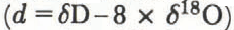
Our data confirm that the geographic distribution of deuterium excess (d) in surface snow in Antarctica exhibits a well-defined pattern from the coast to the interior of the ice sheet, with relatively constant values at around 5‰ in coastal regions, steadily increasing inland, reaching a value of nearly 20‰ in central East Antarctica (see Petit and others, 1991). This distribution may effectively be modeled using a simple Rayleigh model including kinetic effects provided that the temperature of evaporation at the oceanic origin of the air mass and the degree of supersaturation prevailing at snow formation are correctly chosen.
Figure 8a shows the relationship between the deuterium excess and the deuterium content in the 1 m surface snow along the traverse route; this presentation is chosen for the sake of comparison with the results of Reference Petit, White, Young, Jouzel and Korotkevich.Petit and others (1991) shown in Figure 8b. In this graph, we see that the d value is constant around 5‰ while δD values lie between −150‰ and −350‰ (the corresponding temperature range is from −12° to 45°C). When the deuterium and the temperature drop below 400‰ and −50°C, corresponding roughly to the region from the South Pole to Komsomolskaya, the d value clearly shows the previously noted increase (Reference Jouzel and MerlivatJouzel and Merlivat, 1984; Reference Petit, White, Young, Jouzel and Korotkevich.Petit and others, 1991).

Fig. 8. Plots of the excess d versus the deuterium content a. Along the Trans-Antarctica route with a three-order polynomial fitting
Our deuterium-excess results have to be considered as very preliminary, because there is only one measurement at each site and also because a significant measurement uncertainty (± 1–2‰) is attached to each value. These two reasons possibly explain why there is much more scatter along the Trans-Antarctica route than for the data compiled by Reference Petit, White, Young, Jouzel and Korotkevich.Petit and others (1991). Within these limits, the two data sets are remarkably consistent as illustrated by comparing Figures 8a and b (for the sake of this comparison, we have replotted the best-fit curve obtained along the Trans-Antarctica route on Figure 8b).
The main conclusions drawn by Reference Petit, White, Young, Jouzel and Korotkevich.Petit and others (1991) may therefore be extended to the Trans-Antarctica route. According to these authors, the lower d value (5‰) is interpreted as being associated with air masses originating not far from the coast, whereas the higher d values are thought to correspond to all masses from the warmer ocean of the southern lower to mid-latitude regions. There is indeed some evidence to support such an interpretation. Some of the samples which were collected during the Trans-Antarctica Expedition have been processed for chemical analyses. Several results, such as the sea salt and the methane-sulfonic acid (paper in preparation by Qin Dahe and others), independently suggest that the snow falling on the Antarctic Plateau is from a relatively warm ocean in the southern lower to mid-latitude regions.
One interesting approach would be to discover whether there is some correspondence between the change in the isotope temperature gradient, east and west of Vostok, and the spatial distribution of the deuterium excess, which could be expected if there was a link between this isotope gradient and differing characteristics of the regions where the precipitation originates. We await new and more accurate data along the Trans-Antarctica route to explore fully this promising research direction.
6. Conclusions
The relationship between δD and elevation shows two linear relations, one from Patriot Hilk to Vostok and the other from Komsomolskaya to Mirny. In the segment from Vostok to Komsomokkaya, there is a continuous change in δD and 18O, although the altitude remains at about 3500 m a.s.l. throughout.
The difference in δD lines on the two sides of Vostok probably reflect different water sources or different fractionation processes. To confirm this result more evidence is needed, using meteorological observations, glacial chemistry studies or more accurate information on the deuterium-excess distribution.
Although the results concerning this last parameter must be considered as preliminary, they quite remarkably confirm the previously noted features of relatively constant values (around 5‰) for δD lower than −350‰ and of a rapid increase when the elevation is over 3000 m a.s.l., especially in the core region of Antarctica, at the top of the Antarctic Plateau.
Finally, thk study illustrates well the need for more work on the distribution of stable isotopes in Antarctica surface snow and warrants a co-ordinated international effort over the next few years to achieve a comprehensive coverage of the Antarctic continent. The study also shows the advantages of using a combination of isotopic models for data/model comparisons ranging from dynamically simple Rayleigh-type models to more complex three-dimensional isotopic models.
Acknowledgements
This project was supported by the National Committee for Antarctica Research of China (NCAR of China), the National Committee of Science and Technology of China (NCST of China) and National Natural Science Foundations of China (NNSF of China). The other team members, W. Steger (U.S.A.), J. L. Etienne (France), V. Boyarski (U.S.S.R.), G. Somers (U.K.) and K. Funatzu (Japan) were of great help during the field period. The staff of the offices of the 1990 International Trans-Antarctica Expedition and the Soviet Antarctic Expedition provided logistic support and transported the snow samples to Grenoble, France. We thank the French Atomic Energy Agency (CEA, Saclay) for isotopic measurements. We also thank Dr. E.J. Zeller and Dr. G. Dreschhoff for discussions and English corrections, as well as C. Genthon and R. Koster for providing Figures 4 and 5, P. Ciais and V. Lipenkov, for providing unpublished isotope data, and D. Fisher and an anonymous reviewer for their careful reviews.
The accuracy of references in the text and in this list is the responsibility of the authors, to whom queries should be addressed.


